Event-Related Coherence in Visual Cortex and Brain Noise: An MEG Study


1
Centre for Biomedical Technology, Technical University of Madrid, 28223 Madrid, Spain
2
Centre for Technologies in Robotics and Mechatronics Components, Innopolis University, 420500 Innopolis, Russia
*
Author to whom correspondence should be addressed.
†
These authors contributed equally to this work.
Appl. Sci. 2021, 11(1), 375; https://0-doi-org.brum.beds.ac.uk/10.3390/app11010375
Submission received: 12 November 2020
/
Revised: 27 December 2020
/
Accepted: 30 December 2020
/
Published: 2 January 2021
(This article belongs to the Special Issue Advances in Neuroimaging Data Processing)
Abstract
:The analysis of neurophysiological data using the two most widely used open-source MATLAB toolboxes, FieldTrip and Brainstorm, validates our hypothesis about the correlation between event-related coherence in the visual cortex and neuronal noise. The analyzed data were obtained from magnetoencephalography (MEG) experiments based on visual perception of flickering stimuli, in which fifteen subjects effectively participated. Before coherence and brain noise calculations, MEG data were first transformed from recorded channel data to brain source waveforms by solving the inverse problem. The inverse solution was obtained for a 2D cortical shape in Brainstorm and a 3D volume in FieldTrip. We found that stronger brain entrainment to the visual stimuli concurred with higher brain noise in both studies.
1. Introduction
The human brain is a complex network consisting of approximately 86 billion neurons [1] subdivided into oscillatory clusters that fire co-dependently/independently to manifest our consciousness as we know it. These clusters correspond to regions of the brain specialized in processing certain types of information and are connected to other specialized regions in complex networks.
Brain connectivity is studied in three forms: functional, structural, and effective [2,3,4,5]. Structural connectivity identifies anatomical neural networks that show possible pathways for neural communication [6,7]. Functional connectivity finds active brain regions that have a correlated frequency, phase, and/or amplitude [8]. Effective connectivity utilizes the functional connectivity information and additionally determines the direction of the dynamic information flow [9,10]. Effective and functional connectivity can be measured in the frequency domain (e.g., coherence [11]) and in the time domain (e.g., Granger causality [5] or artificial neuronal network-based functional connectivity [12]).
Inter-neuronal communication is realized by one of 50+ neurotransmitters that can be either excitatory (e.g., dopamine) or inhibitory (e.g., gamma-Aminobutyric acid (GABA)) [13]. Voltage-gated ion channels on the cell membranes of neurons generate action potentials and periodic membrane potential activity that synchronizes neighboring neurons [14,15]. These neighboring neurons may, in turn, affect other remotely located neurons, creating a network of connectivity. Coherence-based neuronal communications are driven by the dynamics of neurotransmitters such as amino acid glutamate and GABA.
Only when the synchronous neuronal population is large enough, the produced electrical activity and the concomitant magnetic activity is strong enough to be detected outside the skull using methods such as electroencephalography (EEG) and magnetoencephalography (MEG), respectively [16]. MEG measures the ionic currents inside the neuron (primary currents), whereas EEG measures the return or volume currents outside the neuron (secondary currents).
Coherence is commonly used to quantify neuronal synchronicity between spatially separated EEG electrodes or MEG coils [17]. It is essentially an estimate of the consistency of the relative amplitude and phase between two signals within a given frequency band. There is a linear mathematical method resulting in a symmetric matrix, lacking any directional information. Identical signals produce a coherence magnitude of 1, whereas the coherence magnitude approaches 0 as the dissimilarity between the considered signals increases.
In the last two decades, significant progress has been achieved in the development of new computational algorithms that enable connectivity calculations directly between the different regions of the brain (source space) [5] instead of electrodes or coils (channel space). The source space analysis provides better anatomical localization [18] and enables inter-subject or group analysis as the brain activity now can be projected onto a more standardized space.
In 2004, Hoechstetter et al. [19] introduced a new method to study source coherence in the brain. Discrete multiple source models were created using brain electrical source analysis, and the source activity was transformed into time–frequency space. Finally, magnitude-squared coherence was evaluated to reveal coupled brain sources. The application of inverse solutions to estimate brain activity in the source space from the channel space removes current leakage among adjacent channels. This averts localization errors that are fundamental to coherence analysis in the channel space [19].
Coherence has henceforth been used in many brain connectivity studies on patients and healthy subjects, including but not limited to studies on working memory [20], brain lesions [21], hemiparesis [22], resting-state networks [23], schizophrenia [24,25,26], favorable responses to panic medications [27], and motor imagery [28,29].
Owing to the diversity of human brains, we observe various forms of coherent neuronal activity over different subjects in response to the same flickering stimulus. For example, the presentation of flickering visual stimuli instils coherent responses in the visual cortex at the flicker frequency and its harmonics with varying coherent neuronal network sizes among the subjects [30,31].
Another signal processing technique used to measure synchronization in EEG and MEG is phase synchronization, a measure of how stable the phase difference is over the considered time duration. Phase synchronization requires considered signals to be phase-locked with zero or any finite phase difference, regardless of their respective amplitudes. This is in contrast to the coherence measurement in which phase and amplitude are intertwined for its estimation [32].
Noise, as known [33], can cause desynchronization in a neuronal network. Each participating neuron and interconnecting synapses add to the inherent brain noise when a stimulus is presented to the subject. Therefore, one could argue that a larger neuronal network would carry a higher brain noise and, consequently, lower average coherence. On the other hand, larger active neuronal oscillations in response to the stimulus are likely to have stronger average coherent activity and would also entail higher brain noise. Thus, the relation between the observed coherence and the level of inherent brain noise remains unclear and is the central problem explored in this paper (for comprehensive theoretical descriptions, see [34,35]).
Recently, an approach to estimate inherent brain noise based on phase synchronization was proposed [30]. The method is based on the experiments with flickering images and simultaneous recording of magnetoencephalographic (MEG) data. This paper utilizes the same methodology to measure brain noise using the same experimental paradigm and reveal its correlation with the induced coherence or source power in the visual cortex. We deal with the two most popular open-source MATLAB toolboxes for MEG data analysis, namely FieldTrip [36] and Brainstorm [37], to perform two independent analyses that are more suitable to each software.
2. Materials and Methods
We carried out MEG experiments based on the flickering paradigm with 17 conditionally healthy subjects (age: 17–64 years; 10 males) with normal or corrected-to-normal visual acuity. Two subjects were later discarded. Frequency tags at the stimulus frequency and its harmonics were absent in subject “sub08”, perhaps due to a lack of focus on the experiment. Meanwhile, for subject “sub11”, the ECG activity was not recorded during the experiment due to a technical error, and therefore the signal-to-noise ratio of the subsequently cleaned data was too low to allow correct data analysis. All subjects provided written informed consent before the experiment commencement. The experiments were performed as per the Declaration of Helsinki and approved by the Ethics Committee of the Technical University of Madrid.
2.1. MEG Acquisition
MEG recordings were performed with an Elekta-Neuromag system with 306 channels that was housed in a magnetically shielded room at the Centro de Tecnología Biomédica, Universidad Politécnica de Madrid. The head position was continuously tracked with head position indicator (HPI) coils and co-registered in the device and head coordinate system with three fiducial points (nasion, left, and right preauricular points) and around 300 scalp surface points digitized by a Polhemus Fastrak system. A vertical electrooculogram (EOG) and electrocardiogram (ECG) were placed to capture eye blinks and cardiac activity, respectively. The data were sampled at 1000 Hz.
The experiments for all 17 subjects lasted 4 days. Along with MEG recordings of the subjects, the MEG data were also collected daily in an empty room. All data were passed through an online anti-alias bandpass (0.1–330)-Hz filter. MaxFilter software was used for the temporal signal-space separation (tSSS) to reduce magnetic interference and perform head movement compensation. A 56-ms delay between event triggers and the actual stimulus was measured separately using a photodiode.
2.2. Flickering Stimulation
A grey square image with varying greyness levels on a grey background (brightness: 127 in 8-bit format) was projected onto a translucent screen positioned 150 cm away from the subjects with a 60-Hz frame rate. The pixels’ brightness was modulated by a harmonic signal with frequency Hz (60/9) and a 50% amplitude, i.e., between black (0) and grey (127). This particular frequency was chosen because it produces the most pronounced spectral response in the visual cortex [30].
2.3. Experimental Protocol
The participants were informed about the experimental protocol beforehand in addition to the corresponding textual directives on the screen throughout the experiment. The experiment started with the presentation of a static (non-flickering) square image with a red dot at the center, on which the participant had to concentrate their gaze for 120 s. The recorded brain activity was used as a reference signal or background. After a short rest, the square image started flickering and was presented 2–5 times (depending on the subject) for 120 s, interrupted by a 30-s resting period between each presentation. The flickering stimulus was presented at least 3 times to all subjects except for subject “sub10”. The starting times of the background and flickering recordings were marked with event triggers using a parallel-port setup.
2.4. Analysis Pipelines in FieldTrip and Brainstorm
Next, we will discuss the common steps of the MEG data analysis and related implementation details in both FieldTrip and Brainstorm software. We will focus on the analysis of our experimental data, which, of course, does not cover the full functionality of the two toolboxes.
2.4.1. Reading and Segmenting Data
We start our analysis by reading the MEG data stored in the FIFF format and segmenting them into trials according to experimental conditions. It is common to segment the data after decoding trigger sequences in a raw data file. However, in this work, we make use of additional functions to import events from mat-files in both analyses because there are slight differences in the experimental protocol for some subjects, and this approach is more time-efficient than if-else conditions specifying the subjective exceptions in the batch-processing scripts.
After extracting 120-s epochs for both experimental conditions, including the background activity trial called “B-trial” and event-related trials called “F-trials”, we split every 120-s trial into 4-s (for FieldTrip; see explanation below) or 3-s (for Brainstorm) sub-trials.
2.4.2. Artifact Removal and Loading Data
Accurate brain source analysis requires the correct integration of MEG data with structural magnetic resonance imaging (MRI) scans. Both software programs align all data by defining a subject coordinate system using three fiducial points, namely the nasion and left- and right-auricular points. Moreover, we complemented the alignment based on only three points by an automatic refinement procedure utilizing additional points on the scalp, marked using a 3D digitizer (Polhemus in the considered experiment).
In FieldTrip, we used the “Colin27” head averaged template MRI [38] and adjusted it to the subject’s head shape recorded by the Polhemus device. In Brainstorm, default anatomy was warped to fit the scalp shape of every subject with a 2% fit tolerance using digitized head points from the Polhemus device. After an automatic refinement of head points, the 50-Hz electrical power grid frequency and its harmonics were filtered using notch filters. The 56-ms trigger delay was corrected in the recordings. The recorded electrooculogram (EOG) and electrocardiogram (ECG) signals were used to automatically detect instances of eye blinks and cardiac activity in order to apply signal-space projection (SSP) methods to alleviate the respective artifacts.
Well-defined artifacts such as eye blinks, cardiac activity, muscle contractions, and MEG SQUID jumps were detected semi-automatically using FieldTrip/Brainstorm functions or manual screening. Once artifacts were identified, depending on the artifact intensity, we either discarded trials that contained an artifact or applied linear projection to remove them.
2.4.3. Source Reconstruction
The first step in localizing sources is the construction of a forward model and lead field matrix. The forward model allows one to calculate an estimate of the field measured by the MEG sensors for a given current distribution in the brain and is typically constructed for each subject. The lead fields or the solution to the forward problem are evaluated using various algorithms, such as a single sphere [39], overlapping spheres [40], a spherical harmonics approximation of realistic geometries [41], and boundary element methods [42].
The forward solution was computed in Brainstorm analysis using the overlapping spheres method, which is the default. The number of cortical sources was kept at 15,000 as recommended [37]. On the other hand, in FieldTrip, we applied a semi-realistic head model developed by Nolte [41] called a single-shell model, which is based on the correction of the lead field for a spherical volume conductor by a superposition of basic functions, gradients of harmonic functions constructed from spherical harmonics. We thus discretized the head volume with a grid with a 0.7-cm resolution and obtained a source space consisting of 9025 voxels. The lead field matrix was calculated using each grid point [41]. Thus, in Brainstorm, a cortical surface model was used, and in FieldTrip, a volumetric one.
The next step is calculating the inverse solution to estimate the location and strength of neuronal activity, which can be computed via multiple options, including dipole fitting based on nonlinear optimization [43], minimum variance beamformers in time and frequency domains [44,45,46], and linear estimation of distributed source models [47,48]. In both software analyses, we used standardized low-resolution brain electromagnetic tomography (sLORETA) [49].
The sLORETA family of solutions was validated against numerous imaging modalities [50,51,52] and simulations [53,54]. sLORETA uses standardized current density images to calculate intra-cerebral generators. Although the image was blurred, sLORETA was found [55] to have the exact zero-error localization when reconstructing single sources in all noise-free simulations, i.e., the maximum of the current density power estimate coincided with the exact dipole location [48]. Meanwhile, in all simulations with noise, sLORETA had the lowest localization errors when compared with the minimum norm solution.
Note that when working with multiple sensor types to form a joint source model, the empirical noise covariance is used to compute the weights of each sensor in the overall model. For this purpose, noise covariance matrices are typically computed from empty-room recordings that capture instrumental and environmental noise in the absence of subjects.
2.4.4. Event-Related Coherence
Stimulus-induced coherence in the brain was used to estimate activated brain network size and characterize its activation strength. The taken approach was different for each software program. The previous study with the same stimulus [30] found frequency tags at the flickering frequency (6.67 Hz) and its harmonics. The study also revealed that the frequency tags were more pronounced at the second harmonic (13.33 Hz) than at the first harmonic. Therefore, we need to find an index characterizing the spectral power of brain response at the second harmonic. Since the analysis methods and obtained source models are significantly different, we would require appropriate and independent indices for both software programs to estimate event-related coherence (ERC).
In FieldTrip, we first applied a fourth-order Butterworth 13–14 Hz band-pass filter. The band-pass frequency was determined by the frequency of interest, which in our case was equal to 13.33 Hz (the second harmonic of the flicker frequency). Then, we redefined the 3-s length of every trial within the [0.5, 3.5]-s interval to reduce edge effects due to filtering. Moreover, in this step, we calculated the covariance matrix, necessary when using the sLORETA method. After performing reconstruction of the sources separately for all 3-s B- and F-sub-trials using the sLORETA method, we obtained the power distribution of the activity of the brain sources on the 3D grid with 9025 voxels for every sub-trial.
In the next step, we averaged the resulting source power distributions and obtained a distribution each for B- and F-condition ( and ). Such an approach made it possible to reduce the influence of instrumental and brain noise on the results of source reconstruction and, thus, increase the prominence of the event-related pattern of neural activity, compared to source reconstruction based on a single original 120-s trial. After that, we calculated the normalized difference of the source power distributions for F- and B-conditions (so-called baseline correction): . This procedure was needed to isolate the event-related pattern of source activity. The above steps were repeated for three 120-s F-trials (all subjects had at least three F-trials except “sub10”), and the average of the obtained three differences D was calculated. Finally, the distribution of the averaged difference was interpolated on the used MRI image.
In Brainstorm, we started by calculating magnitude-squared coherence between the time series of each of the 15,000 brain sources and the reference sinusoidal signal at frequency (13.33 Hz), i.e., the second harmonic of the flicker frequency, for both the F-trials () and the B-trial (). To evaluate the event-related coherence in the brain, we calculated differences between the coherence values of the F-trials and B-trials for cortical sources lying in visual areas and as per the Brodmann atlas, , and averaged it for each subject.
2.5. Brain Noise Estimation
The proposed brain noise estimation method is based on phase synchronization, which implies a measurement of a phase difference between the brain’s response in the visual cortex and the reference signal at the second harmonic frequency ( Hz). First, to obtain the visual response, we averaged the source activity waveforms from the and subregions of the Brodmann atlas for each of the F-trials of a subject. We then bandpass-filtered this average visual response in the 13–14 Hz frequency band. To estimate brain noise, we calculated the phase difference time series between visual response time series and the second harmonic of the flicker sinusoidal signal, as [30,56]:
where and are the times of nth maxima of the visual response time series and the second harmonic of the flicker signal, respectively. Intermittent frequency-locking was observed, superposed with random fluctuations due to phase noise [33]. We also obtained unimodal probability distributions of these phase differences to characterize the phase-noise-induced random fluctuations in phase. Kurtosis, a measure of the sharpness of a unimodal distribution, would be lower for a broader and noisier phase fluctuation distribution, and vice versa. Therefore, from the probability distribution of these random phase fluctuations, we estimated brain noise as the inverse distribution’s kurtosis. This method was comprehensively described in the previous paper [30].
3. Results
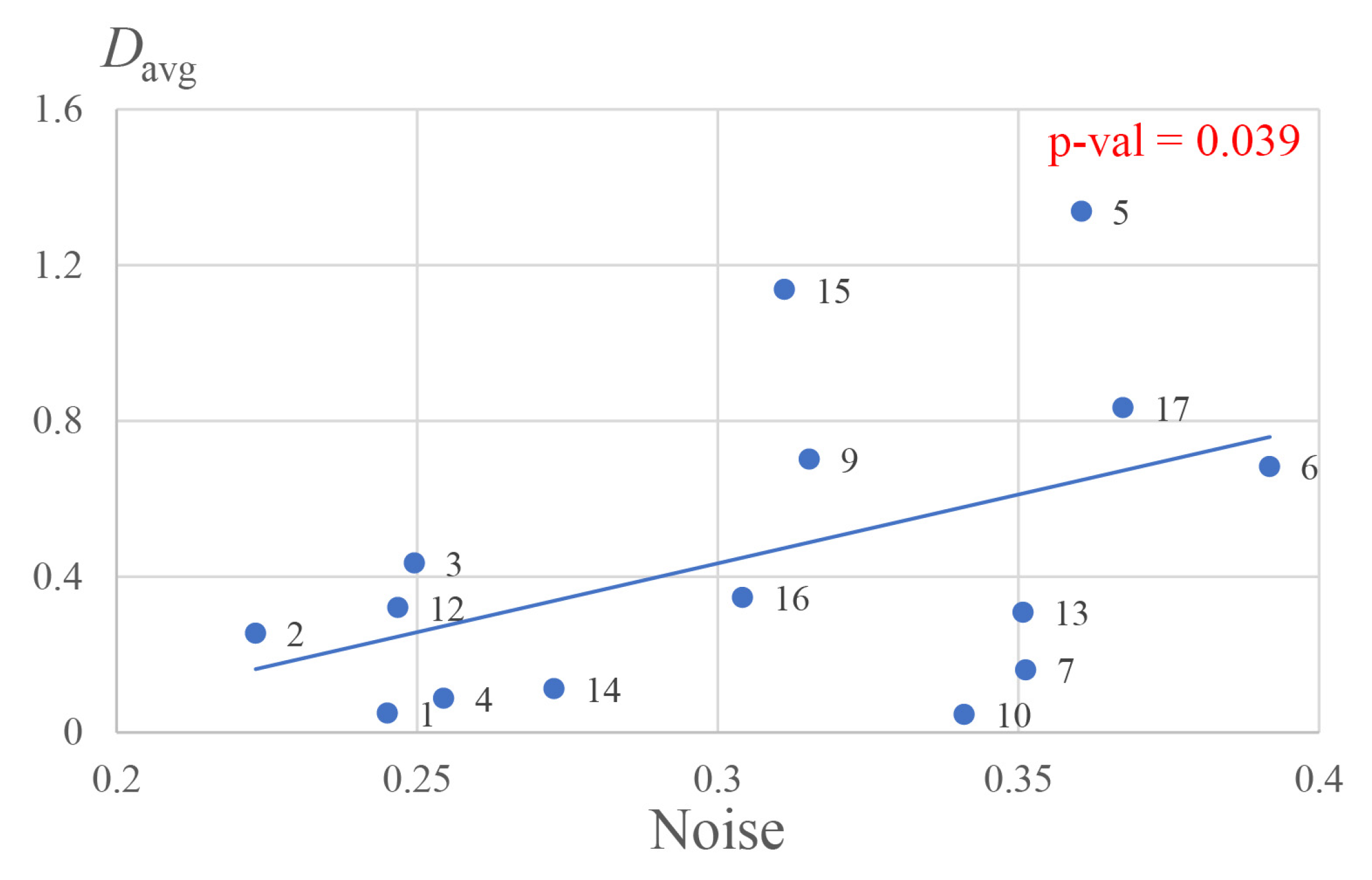
Based on the obtained normalized distributions of the source power, we calculated for each subject the average power of source activity in the visual cortex, , in FieldTrip. It should be noted that we determined the visual cortex using the automated anatomical labeling (AAL) brain atlas [57] in FieldTrip. The average spectral power in the visual cortex was plotted in Figure 1 against estimated brain noise to phase synchronization (in units of inverse kurtosis) for every subject.
One can see a linear correlation (with p-value equal to 0.039 and an -value of ) of and noise level, although the scatter is significant: , ; , .
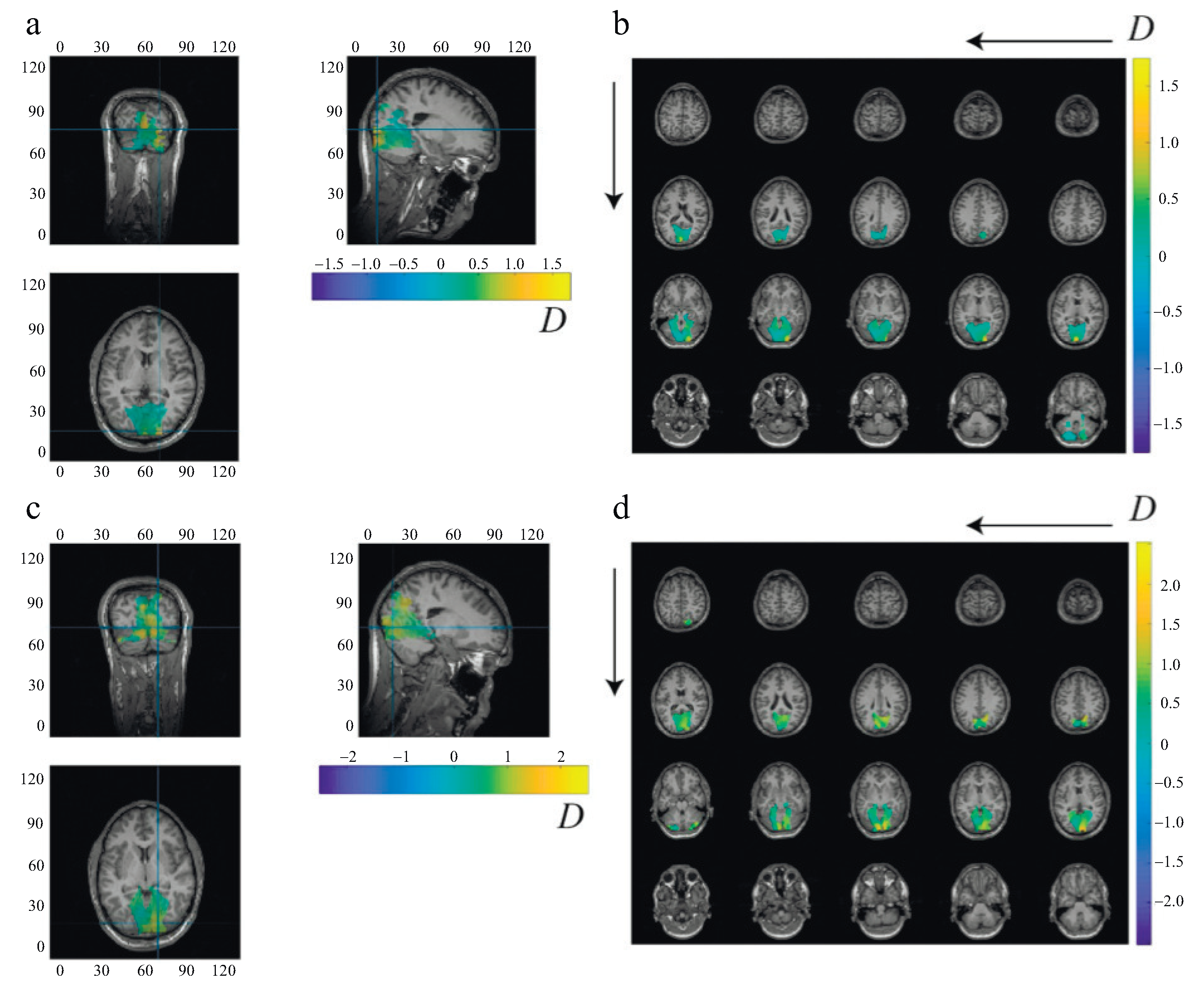
Figure 2 shows typical distributions of normalized source power D predominantly activated within the visual cortex for subjects with low (subject 2) and high (subject 6) brain noise. Subject 6 is characterized by more pronounced high-amplitude activity spanning a larger volume in the visual cortex than subject 2.
We will show now the results of the alternate analysis pipeline in Brainstorm. The values of average event-related coherence over visual areas V1 and V2 were compared with the same estimated brain noise as used in Figure 1 for all subjects. A linear relation was established with a p-value of and an -value of , as seen in Figure 3. The distributions of average event-related coherence over the cortex for typical subjects with low and high noise levels are shown in Figure 4 as per the cortical analysis in Brainstorm.
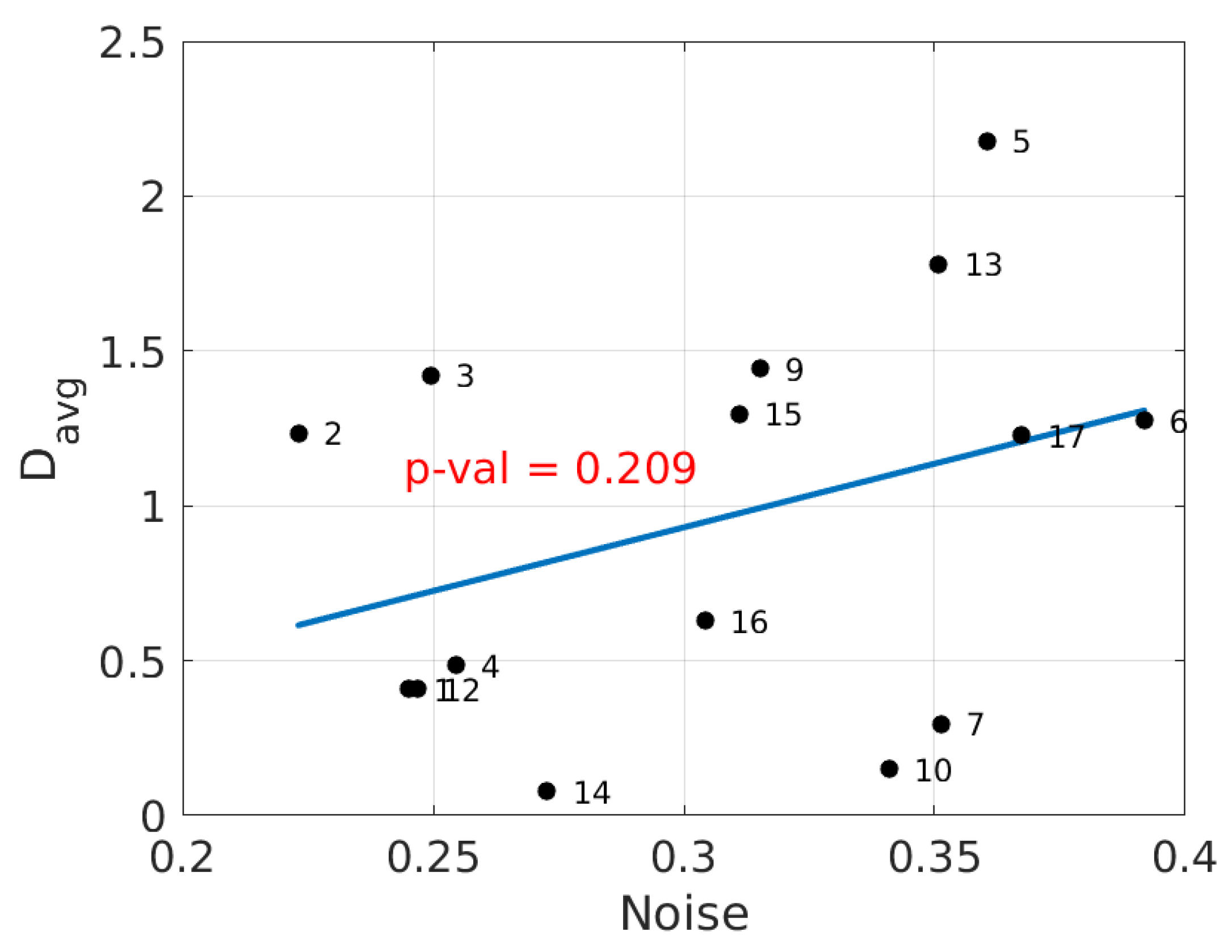
The methodology to calculate the normalized difference of power on a 3D volume in FieldTrip was adapted to fit the 2D source model generated in Brainstorm to have a closer comparison. Figure 5 shows the corresponding linear regression model with a p-value of and an -value of (, ; , ). Although the model fails to capture any significant relation, the relative positions of the subjects in the power–noise state-space of Figure 5 are quite similar to those which we observe in Figure 1.
4. Discussion
We found a linear relation, with a positive slope between the average power of source activity in the visual cortex and brain noise. The results show that the subjects with more powerful visual cortex activity demonstrate more substantial brain noise. This relationship can be explained as follows. The higher the power of the reconstructed sources, the more neurons are involved in realizing cognitive activity. In a larger network of neurons, the number of synapses would also be higher, and both the synapses and the neurons would feed the phase-destabilizing noise into the system [30].
The two independent methods essentially lead to the calculation of the difference in spectral activity inside the subject’s brain, corresponding to the second harmonic of the stimulus frequency when the subject is observing a flickering image, as opposed to when the subject is gazing at a stationary stimulus. Averaging them over the respective regions of interest led to very similar trends between average event-related coherence or frequency-filtered signal power and brain noise using either software program (Figure 1 and Figure 3). One can see in Figure 2 and Figure 4 that the subject with higher brain noise (“sub06”) has a more extensive and intensely activated neuronal network, coherent with the stimulus, as distinct from the subject with lower brain noise (“sub02”).
As we have already mentioned above, we set out to adapt the prescribed analysis pipelines of both FieldTrip and Brainstorm to our study. The two software programs gave congruent results following their independent analysis strategies. However, it should not be a surprise that if we try mixing the two analysis pipelines midway, the results will likely deteriorate. Figure 5 shows the result of such mindless mixing of the two methods. Even though the order of subjects’ frequency-filtered signal powers remained conserved from Figure 1, the linear relation was lost.
Since we calculate brain noise from the phase fluctuation time series and the corresponding probability distribution, which in turn depends upon the signal-to-noise ratio (SNR) of the source waveforms in the visual cortex to be properly calculated, it can turn into a circular problem where, for very high brain noises, the SNR would be too low to correctly determine the phase fluctuations, which would make the calculation of brain noise impossible. This was the case with subjects “sub8” and “sub11”. For these subjects, we did not see any frequency tags in the power spectrum during the flickering cube presentation (signal) and also in the power spectrum for the stationary cube presentation (noise). Thus, they had to be removed from the study. The subjects who showed frequency tags in the power spectrum also had clear bandpass-filtered waveforms in the 13–14 Hz frequency band used to calculate phase difference fluctuations.
We have to emphasize that all codes of our analysis and MEG data used for this study were made publicly available during the review period. The developed methods, along with the prescribed codes on the software documentations adapted to a generic MEG study starting with only a FIFF file, will be accessible to newcomers in the field.
5. Conclusions
Visual flickering experiments were carried out successfully with fifteen healthy subjects, and their brain responses were recorded using MEG. The two most popular open-source software programs, FieldTrip and Brainstorm, were used to analyze brain source activity. We calculated the event-related coherence of the brain response with the flickering visual signal. Using a recently proposed brain noise estimation method, we computed the relation between the coherent brain network in the visual cortex and corresponding brain noise. The results obtained by the two software programs demonstrated fair agreement. The analyses performed by both MATLAB toolboxes evidenced that more extensive brain activity is accompanied by more substantial brain noise.
Author Contributions
Conceptualization, P.C. and S.A.K.; methodology, A.N.P. and A.E.H.; software, P.C. and S.A.K.; validation, A.N.P. and A.E.H.; formal analysis, all authors; investigation, A.N.P. and A.E.H.; resources, A.N.P.; data curation, P.C.; writing—original draft preparation, P.C. and S.A.K.; writing—review and editing, all authors; visualization, P.C. and S.A.K.; supervision, A.N.P. and A.E.H.; project administration, A.N.P. and A.E.H.; funding acquisition, A.N.P. and A.E.H. All authors have read and agreed to the published version of the manuscript.
Funding
This research was funded by the Spanish Ministry of Economy and Competitiveness SAF2016-80240 in the part of the experimental study and Russian Science Foundation No. 19-12-00050 in the part of the data processing. S.A.K. is supported by the President Program (MD-1921.2020.9) in the part of the source reconstruction.
Institutional Review Board Statement
The study was conducted according to the guidelines of the Declaration of Helsinki, and approved by the Ethics Committee of the Technical University of Madrid (protocol No. 19, 3 February 2020).
Informed Consent Statement
Informed consent was obtained from all subjects involved in the study.
Data Availability Statement
The MEG data have been uploaded at https://zenodo.org/record/4408648#.X-72UdYo-Cc. Both FieldTrip and Brainstorm codes have been uploaded as a single release at https://zenodo.org/record/4408756#.X-77itYo-Cc.
Acknowledgments
The authors graciously acknowledge the subjects for their contribution to this research.
Conflicts of Interest
The authors declare no conflict of interest. The funders had no role in the design of the study; in the collection, analyses, or interpretation of data; in the writing of the manuscript, or in the decision to publish the results.
References
- Azevedo, F.A.C.; Carvalho, L.R.B.; Grinberg, L.T.; Farfel, J.M.; Ferretti, R.E.L.; Leite, R.E.P.; Jacob Filho, W.; Lent, R.; Herculano-Houzel, S. Equal numbers of neuronal and nonneuronal cells make the human brain an isometrically scaled-up primate brain. J. Comp. Neurol. 2009, 513, 532–541. [Google Scholar] [CrossRef] [PubMed]
- Friston, K.J.; Frith, C.D.; Liddle, P.F.; Frackowiak, R.S. Functional connectivity: The principal-component analysis of large (PET) data sets. J. Cereb. Blood Flow Metab. 1993, 13, 5–14. [Google Scholar] [CrossRef] [PubMed]
- Greenblatt, R.E.; Pflieger, M.E.; Ossadtchi, A.E. Connectivity measures applied to human brain electrophysiological data. J. Neurosci. Methods 2012, 207, 1–16. [Google Scholar] [CrossRef] [PubMed] [Green Version]
- Sakkalis, V. Review of advanced techniques for the estimation of brain connectivity measured with EEG/MEG. Comput. Biol. Med. 2011, 41, 1110–1117. [Google Scholar] [CrossRef] [PubMed]
- Hramov, A.E.; Frolov, N.S.; Maksimenko, V.A.; Kurkin, S.A.; Kazantsev, V.B.; Pisarchik, A.N. Functional networks of the brain: From connectivity restoration to dynamic integration. Phys. Uspekhi 2020, 63. [Google Scholar] [CrossRef]
- Le Bihan, D.; Mangin, J.F.; Poupon, C.; Clark, C.A.; Pappata, S.; Molko, N.; Chabriat, H. Diffusion tensor imaging: Concepts and applications. J. Magn. Reson. Imaging JMRI 2001, 13, 534–546. [Google Scholar] [CrossRef]
- Wedeen, V.J.; Wang, R.P.; Schmahmann, J.D.; Benner, T.; Tseng, W.Y.I.; Dai, G.; Pandya, D.N.; Hagmann, P.; D’Arceuil, H.; de Crespigny, A.J. Diffusion spectrum magnetic resonance imaging (DSI) tractography of crossing fibers. NeuroImage 2008, 41, 1267–1277. [Google Scholar] [CrossRef]
- Towle, V.L.; Hunter, J.D.; Edgar, J.C.; Chkhenkeli, S.A.; Castelle, M.C.; Frim, D.M.; Kohrman, M.; Hecox, K.E. Frequency Domain Analysis of Human Subdural Recordings. J. Clin. Neurophysiol. 2007, 24, 205–213. [Google Scholar] [CrossRef]
- Cabral, J.; Kringelbach, M.L.; Deco, G. Exploring the network dynamics underlying brain activity during rest. Prog. Neurobiol. 2014, 114, 102–131. [Google Scholar] [CrossRef] [Green Version]
- Horwitz, B. The elusive concept of brain connectivity. NeuroImage 2003, 19, 466–470. [Google Scholar] [CrossRef]
- Bowyer, S.M. Coherence a measure of the brain networks: Past and present. Neuropsychiatr. Electrophysiol. 2016, 2, 1. [Google Scholar] [CrossRef]
- Frolov, N.; Maksimenko, V.; Lüttjohann, A.; Koronovskii, A.; Hramov, A. Feed-forward artificial neural network provides data-driven inference of functional connectivity. Chaos Interdiscip. J. Nonlinear Sci. 2019, 29, 091101. [Google Scholar] [CrossRef] [PubMed]
- Chana, G.; Bousman, C.A.; Money, T.T.; Gibbons, A.; Gillett, P.; Dean, B.; Everall, I.P. Biomarker investigations related to pathophysiological pathways in schizophrenia and psychosis. Front. Cell. Neurosci. 2013, 7. [Google Scholar] [CrossRef] [PubMed] [Green Version]
- Llinás, R.R. The intrinsic electrophysiological properties of mammalian neurons: Insights into central nervous system function. Science 1988, 242, 1654–1664. [Google Scholar] [CrossRef]
- Llinás, R.R.; Grace, A.A.; Yarom, Y. In vitro neurons in mammalian cortical layer 4 exhibit intrinsic oscillatory activity in the 10- to 50-Hz frequency range. Proc. Natl. Acad. Sci. USA 1991, 88, 897–901. [Google Scholar] [CrossRef] [Green Version]
- Hämäläinen, M.; Hari, R.; Ilmoniemi, R.J.; Knuutila, J.; Lounasmaa, O.V. Magnetoencephalography—Theory, instrumentation, and applications to noninvasive studies of the working human brain. Am. Phys. Soc. 1993, 65. [Google Scholar] [CrossRef] [Green Version]
- French, C.C.; Beaumont, J.G. A critical review of EEG coherence studies of hemisphere function. Int. J. Psychophysiol. Off. J. Int. Organ. Psychophysiol. 1984, 1, 241–254. [Google Scholar] [CrossRef]
- Kurkin, S.; Hramov, A.; Chholak, P.; Pisarchik, A. Localizing oscillatory sources in a brain by MEG data during cognitive activity. In Proceedings of the 2020 4th International Conference on Computational Intelligence and Networks (CINE), Kolkata, India, 27–29 February 2020; pp. 1–4. [Google Scholar]
- Hoechstetter, K.; Bornfleth, H.; Weckesser, D.; Ille, N.; Berg, P.; Scherg, M. BESA source coherence: A new method to study cortical oscillatory coupling. Brain Topogr. 2004, 16, 233–238. [Google Scholar] [CrossRef]
- Gross, J.; Schmitz, F.; Schnitzler, I.; Kessler, K.; Shapiro, K.; Hommel, B.; Schnitzler, A. Modulation of long-range neural synchrony reflects temporal limitations of visual attention in humans. Proc. Natl. Acad. Sci. USA 2004, 101, 13050–13055. [Google Scholar] [CrossRef] [Green Version]
- Guggisberg, A.G.; Honma, S.M.; Findlay, A.M.; Dalal, S.S.; Kirsch, H.E.; Berger, M.S.; Nagarajan, S.S. Mapping functional connectivity in patients with brain lesions. Ann. Neurol. 2008, 63, 193–203. [Google Scholar] [CrossRef] [Green Version]
- Belardinelli, P.; Ciancetta, L.; Staudt, M.; Pizzella, V.; Londei, A.; Birbaumer, N.; Romani, G.L.; Braun, C. Cerebro-muscular and cerebro-cerebral coherence in patients with pre- and perinatally acquired unilateral brain lesions. NeuroImage 2007, 37, 1301–1314. [Google Scholar] [CrossRef] [PubMed]
- De Pasquale, F.; Della Penna, S.; Snyder, A.Z.; Lewis, C.; Mantini, D.; Marzetti, L.; Belardinelli, P.; Ciancetta, L.; Pizzella, V.; Romani, G.L.; et al. Temporal dynamics of spontaneous MEG activity in brain networks. Proc. Natl. Acad. Sci. USA 2010, 107, 6040–6045. [Google Scholar] [CrossRef] [PubMed] [Green Version]
- Hinkley, L.B.N.; Vinogradov, S.; Guggisberg, A.G.; Fisher, M.; Findlay, A.M.; Nagarajan, S.S. Clinical symptoms and alpha band resting-state functional connectivity imaging in patients with schizophrenia: Implications for novel approaches to treatment. Biol. Psychiatry 2011, 70, 1134–1142. [Google Scholar] [CrossRef] [PubMed] [Green Version]
- Kim, J.S.; Shin, K.S.; Jung, W.H.; Kim, S.N.; Kwon, J.S.; Chung, C.K. Power spectral aspects of the default mode network in schizophrenia: An MEG study. BMC Neurosci. 2014, 15, 104. [Google Scholar] [CrossRef] [Green Version]
- Bowyer, S.M.; Gjini, K.; Zhu, X.; Kim, L.; Moran, J.E.; Rizvi, S.U.; Gumenyuk, N.T.; Tepley, N.; Boutros, N.N. Potential Biomarkers of Schizophrenia from MEG Resting-State Functional Connectivity Networks: Preliminary Data. J. Behav. Brain Sci. 2015, 5, 1. [Google Scholar] [CrossRef] [Green Version]
- Boutros, N.N.; Galloway, M.P.; Ghosh, S.; Gjini, K.; Bowyer, S.M. Abnormal coherence imaging in panic disorder: A magnetoencephalography investigation. Neuroreport 2013, 24, 487–491. [Google Scholar] [CrossRef]
- Chholak, P.; Pisarchik, A.N.; Kurkin, S.A.; Maksimenko, V.A.; Hramov, A.E. Neuronal pathway and signal modulation for motor communication. Cybern. Phys. 2019, 106–113. [Google Scholar] [CrossRef] [Green Version]
- Chholak, P.; Niso, G.; Maksimenko, V.A.; Kurkin, S.A.; Frolov, N.S.; Pitsik, E.N.; Hramov, A.E.; Pisarchik, A.N. Visual and kinesthetic modes affect motor imagery classification in untrained subjects. Sci. Rep. 2019, 9, 1–12. [Google Scholar]
- Pisarchik, A.N.; Chholak, P.; Hramov, A.E. Brain noise estimation from MEG response to flickering visual stimulation. Chaos Solitons Fractals X 2019, 100005. [Google Scholar] [CrossRef]
- Chholak, P.; Maksimenko, V.A.; Hramov, A.E.; Pisarchik, A.N. Voluntary and involuntary attention in bistable visual perception: A MEG study. Front. Hum. Neurosci. 2020, 14, 555. [Google Scholar]
- Uhlhaas, P.J.; Roux, F.; Rodriguez, E.; Rotarska-Jagiela, A.; Singer, W. Neural synchrony and the development of cortical networks. Trends Cogn. Sci. 2010, 14, 72–80. [Google Scholar] [CrossRef] [PubMed]
- Boccaletti, S.; Pisarchik, A.; Genio, C.; Amann, A. Synchronization: From Coupled Systems to Complex Networks; Cambridge University Press: Cambridge, UK, 2018. [Google Scholar] [CrossRef]
- Chholak, P.; Hramov, A.E.; Pisarchik, A.N. An advanced perception model combining brain noise and adaptation. Nonlinear Dyn. 2020, 100, 3695–3709. [Google Scholar] [CrossRef]
- An, P.; Va, M.; Av, A.; Ns, F.; Vv, M.; Mo, Z.; Ae, R.; Ae, H. Coherent resonance in the distributed cortical network during sensory information processing. Sci. Rep. 2019, 9, 18325. [Google Scholar] [CrossRef] [Green Version]
- Oostenveld, R.; Fries, P.; Maris, E.; Schoffelen, J.M. FieldTrip: Open Source Software for Advanced Analysis of MEG, EEG, and Invasive Electrophysiological Data. Comput. Intell. Neurosci. 2010, 2011, e156869. [Google Scholar] [CrossRef]
- Tadel, F.; Baillet, S.; Mosher, J.C.; Pantazis, D.; Leahy, R.M. Brainstorm: A user-friendly application for MEG/EEG analysis. Comput. Intell. Neurosci. 2011, 2011, 879716. [Google Scholar] [CrossRef]
- Holmes, C.J.; Hoge, R.; Collins, L.; Woods, R.; Toga, A.W.; Evans, A.C. Enhancement of MR images using registration for signal averaging. J. Comput. Assist. Tomogr. 1998, 22, 324–333. [Google Scholar] [CrossRef]
- Cuffin, B.N.; Cohen, D. Magnetic fields of a dipole in special volume conductor shapes. IEEE Trans. Bio-Med. Eng. 1977, 24, 372–381. [Google Scholar] [CrossRef]
- Huang, M.X.; Mosher, J.C.; Leahy, R.M. A sensor-weighted overlapping-sphere head model and exhaustive head model comparison for MEG. Phys. Med. Biol. 1999, 44, 423–440. [Google Scholar] [CrossRef]
- Nolte, G. The magnetic lead field theorem in the quasi-static approximation and its use for magnetoencephalography forward calculation in realistic volume conductors. Phys. Med. Biol. 2003, 48, 3637–3652. [Google Scholar] [CrossRef]
- Darvas, F.; Pantazis, D.; Kucukaltun-Yildirim, E.; Leahy, R.M. Mapping human brain function with MEG and EEG: Methods and validation. NeuroImage 2004, 23, S289–S299. [Google Scholar] [CrossRef]
- Scherg, M. Fundamentals of dipole source analysis. Adv. Audiol. 1990, 6, 40–69. [Google Scholar]
- Van Veen, B.D.; Van Drongelen, W.; Yuchtman, M.; Suzuki, A. Localization of brain electrical activity via linearly constrained minimum variance spatial filtering. IEEE Trans. Bio-Med. Eng. 1997, 44, 867–880. [Google Scholar] [CrossRef] [PubMed]
- Gross, J.; Kujala, J.; Hämäläinen, M.; Timmermann, L.; Schnitzler, A.; Salmelin, R. Dynamic imaging of coherent sources: Studying neural interactions in the human brain. Proc. Natl. Acad. Sci. USA 2001, 98, 694–699. [Google Scholar] [CrossRef] [PubMed] [Green Version]
- Kurkin, S.; Chholak, P.; Pisarchik, A.; Hramov, A. Analysis of the features of brain neuronal sources during imagery motor activity: MEG study. In Proceedings of the 2020 4th Scientific School on Dynamics of Complex Networks and their Application in Intellectual Robotics (DCNAIR), Innopolis, Russia, 7–9 September 2020; pp. 154–157. [Google Scholar]
- Hämäläinen, M.S.; Ilmoniemi, R.J. Interpreting magnetic fields of the brain: Minimum norm estimates. Med. Biol. Eng. Comput. 1994, 32, 35–42. [Google Scholar] [CrossRef]
- Grech, R.; Cassar, T.; Muscat, J.; Camilleri, K.P.; Fabri, S.G.; Zervakis, M.; Xanthopoulos, P.; Sakkalis, V.; Vanrumste, B. Review on solving the inverse problem in EEG source analysis. J. Neuroeng. Rehabil. 2008, 5, 25. [Google Scholar] [CrossRef] [Green Version]
- Pascual-Marqui, R.D. Standardized low-resolution brain electromagnetic tomography (sLORETA): Technical details. Methods Find. Exp. Clin. Pharmacol. 2002, 24, 5–12. [Google Scholar]
- Mulert, C.; Jäger, L.; Schmitt, R.; Bussfeld, P.; Pogarell, O.; Möller, H.J.; Juckel, G.; Hegerl, U. Integration of fMRI and simultaneous EEG: Towards a comprehensive understanding of localization and time-course of brain activity in target detection. NeuroImage 2004, 22, 83–94. [Google Scholar] [CrossRef]
- Zumsteg, D.; Friedman, A.; Wieser, H.G.; Wennberg, R.A. Propagation of interictal discharges in temporal lobe epilepsy: Correlation of spatiotemporal mapping with intracranial foramen ovale electrode recordings. Clin. Neurophysiol. 2006, 117, 2615–2626. [Google Scholar] [CrossRef]
- Olbrich, S.; Mulert, C.; Karch, S.; Trenner, M.; Leicht, G.; Pogarell, O.; Hegerl, U. EEG-vigilance and BOLD effect during simultaneous EEG/fMRI measurement. NeuroImage 2009, 45, 319–332. [Google Scholar] [CrossRef]
- Pascual-Marqui, R.D.; Lehmann, D.; Koukkou, M.; Kochi, K.; Anderer, P.; Saletu, B.; Tanaka, H.; Hirata, K.; John, E.R.; Prichep, L.; et al. Assessing interactions in the brain with exact low-resolution electromagnetic tomography. Philos. Trans. R. Soc. Math. Eng. Sci. 2011, 369, 3768–3784. [Google Scholar] [CrossRef]
- Lopes, M.A.; Junges, L.; Tait, L.; Terry, J.R.; Abela, E.; Richardson, M.P.; Goodfellow, M. Computational modelling in source space from scalp EEG to inform presurgical evaluation of epilepsy. Clin. Neurophysiol. 2020, 131, 225–234. [Google Scholar] [CrossRef] [PubMed]
- Pascual-Marqui, R.D.; Esslen, M.; Kochi, K.; Lehmann, D. Functional imaging with low-resolution brain electromagnetic tomography (LORETA): A review. Methods Find. Exp. Clin. Pharmacol. 2002, 24, 91–95. [Google Scholar] [PubMed]
- Pisarchik, A.; Jaimes-Reátegui, R.; Villalobos-Salazar, J.; Garcia-Lopez, J.; Boccaletti, S. Synchronization of chaotic systems with coexisting attractors. Phys. Rev. Lett. 2006, 96, 244102. [Google Scholar] [CrossRef] [PubMed]
- Tzourio-Mazoyer, N.; Landeau, B.; Papathanassiou, D.; Crivello, F.; Etard, O.; Delcroix, N.; Mazoyer, B.; Joliot, M. Automated anatomical labeling of activations in SPM using a macroscopic anatomical parcellation of the MNI MRI single-subject brain. NeuroImage 2002, 15, 273–289. [Google Scholar] [CrossRef]
Figure 1.
The average power of source activity in the brain volume corresponding to visual cortex versus brain noise for all subjects (numbers denote the subjects). The line is a linear approximation fit (, ).
Figure 1.
The average power of source activity in the brain volume corresponding to visual cortex versus brain noise for all subjects (numbers denote the subjects). The line is a linear approximation fit (, ).

Figure 2.
Distributions of normalized source power D within the visual cortex plotted superimposed on anatomical MRI in orthogonal cut view (a,c) and slice mode (b,d) for subject 2 (a,b) and subject 6 (c,d). The blue crosses in (a,c) define the cutting planes. The arrows in (b,d) indicate the direction of movement along the slices.

Figure 3.
Average event-related coherence in the visual cortex versus estimated brain noise to phase synchronization. The straight line is a linear regression fit of the data (, ).
Figure 3.
Average event-related coherence in the visual cortex versus estimated brain noise to phase synchronization. The straight line is a linear regression fit of the data (, ).

Figure 4.
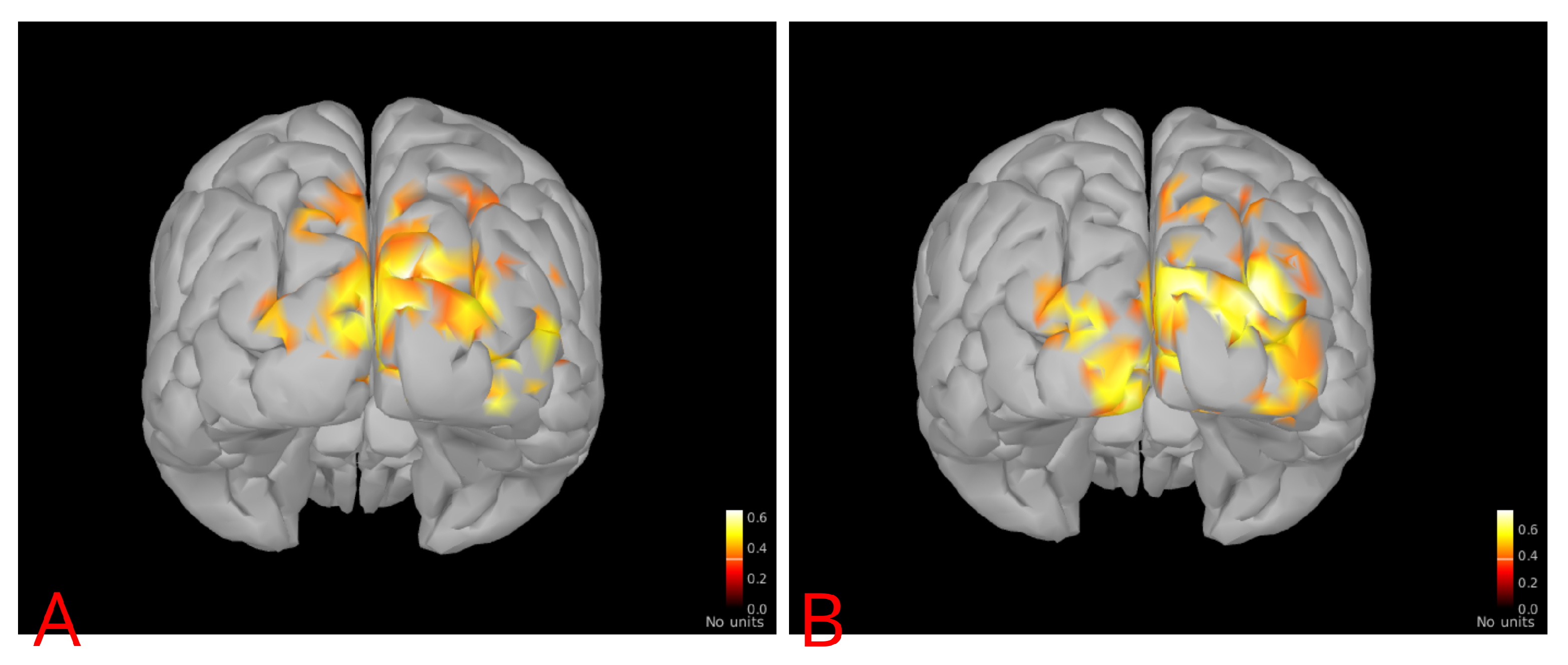
Typical cortical distributions of event-related coherence for (A) Subject 2 (low noise) and (B) Subject 6 (high noise). The brain activation is more intensive in the latter case.
Figure 4.
Typical cortical distributions of event-related coherence for (A) Subject 2 (low noise) and (B) Subject 6 (high noise). The brain activation is more intensive in the latter case.

Figure 5.
The average power of source activity in the visual cortex versus brain noise for all subjects (numbers denote the subjects). The line is a linear approximation fit (, ).
Figure 5.
The average power of source activity in the visual cortex versus brain noise for all subjects (numbers denote the subjects). The line is a linear approximation fit (, ).

Publisher’s Note: MDPI stays neutral with regard to jurisdictional claims in published maps and institutional affiliations. |
© 2021 by the authors. Licensee MDPI, Basel, Switzerland. This article is an open access article distributed under the terms and conditions of the Creative Commons Attribution (CC BY) license (http://creativecommons.org/licenses/by/4.0/).
Share and Cite
MDPI and ACS Style
Chholak, P.; Kurkin, S.A.; Hramov, A.E.; Pisarchik, A.N. Event-Related Coherence in Visual Cortex and Brain Noise: An MEG Study. Appl. Sci. 2021, 11, 375. https://0-doi-org.brum.beds.ac.uk/10.3390/app11010375
AMA Style
Chholak P, Kurkin SA, Hramov AE, Pisarchik AN. Event-Related Coherence in Visual Cortex and Brain Noise: An MEG Study. Applied Sciences. 2021; 11(1):375. https://0-doi-org.brum.beds.ac.uk/10.3390/app11010375
Chicago/Turabian StyleChholak, Parth, Semen A. Kurkin, Alexander E. Hramov, and Alexander N. Pisarchik. 2021. "Event-Related Coherence in Visual Cortex and Brain Noise: An MEG Study" Applied Sciences 11, no. 1: 375. https://0-doi-org.brum.beds.ac.uk/10.3390/app11010375
Note that from the first issue of 2016, this journal uses article numbers instead of page numbers. See further details here.