Article

Distracted and Drowsy Driving Modeling Using Deep Physiological Representations and Multitask Learning

Department of Computer Science and Engineering, University of Michigan, Ann Arbor, MI 48109, USA
*
Authors to whom correspondence should be addressed.
Submission received: 18 November 2020 / Revised: 11 December 2020 / Accepted: 19 December 2020 / Published: 24 December 2020
(This article belongs to the Special Issue Pattern Recognition in Multimedia Signal Analysis)

Abstract

:
In this paper, we investigated various physiological indicators on their ability to identify distracted and drowsy driving. In particular, four physiological signals are being tested: blood volume pulse (BVP), respiration, skin conductance and skin temperature. Data were collected from 45 participants, under a simulated driving scenario, through different times of the day and during their engagement on a variety of physical and cognitive distractors. We explore several statistical features extracted from those signals and their efficiency to discriminate between the presence or not of each of the two conditions. To that end, we evaluate three traditional classifiers (Random Forests, KNN and SVM), which have been extensively applied by the related literature and we compare their performance against a deep CNN-LSTM network that learns spatio-temporal physiological representations. In addition, we explore the potential of learning multiple conditions in parallel using a single machine learning model, and we discuss how such a problem could be formulated and what are the benefits and disadvantages of the different approaches. Overall, our findings indicate that information related to the BVP data, especially features that describe patterns with respect to the inter-beat-intervals (IBI), are highly associates with both targeted conditions. In addition, features related to the respiratory behavior of the driver can be indicative of drowsiness, while being less associated with distractions. Moreover, spatio-temporal deep methods seem to have a clear advantage against traditional classifiers on detecting both driver conditions. Our experiments show, that even though learning both conditions jointly can not compete directly to individual, task-specific CNN-LSTM models, deep multitask learning approaches have a great potential towards that end as they offer the second best performance on both tasks against all other evaluated alternatives in terms of sensitivity, specificity and the area under the receiver operating characteristic curve (AUC).

1. Introduction

Understanding human behavior is on the epicenter of modern AI research. Modeling and monitoring a user’s state is critical towards designing adaptive and personalized interactions and has lead to ground-braking changes on several domains during the last few years. The transportation sector, in particular, is one of the application areas that have invested the most in “smart” monitoring with the broader goal of increasing safety and improving the quality of the overall experience [1]. That is especially true for the automotive industry, as for many years the number of road accidents has been steadily increasing and car manufacturers have shifted their attention on the search of machine learning and AI-powered solutions.
According to the World Health Organization (WHO), each year 1.35 million people lose their lives to road accidents while 50 million get injured [2,3]. That translates to approximately 3700 deaths and 137,000 injuries daily. Moreover, based on the same resource, road traffic injuries are the leading cause of death for children and young adults between the ages of 5 to 29 years. Particularly, young males are three times more likely to be involved in a car accident than young females, with mobile phone usage being the most common cause of distractions. What is especially surprising according to WHO findings, is that hands-free phone usage remains almost equally dangerous to the physical interaction with the device. It is estimated that road crashes cost most countries an average of 3% of their gross domestic product while future trends show that by 2030, fatalities related to road accidents will be the fifth most common cause of mortality globally, from being ninth in 2011.
Specifically in the US, the National Highway Traffic Safety Administration (NHTSA) reports that only in 2018, 2800 lives were lost and more than 400,000 people were injured due to distracted driving. Additionally, only in 2017, 91,000 police-reported crashes involved drowsy drivers leading to an estimated 50,000 people injured and nearly 800 deaths. However, as the NHTSA suggests, there is broad agreement across the traffic safety, sleep science and public health communities that these numbers are an underestimate of the real impact that driving while being mentally or physically fatigued can have. An underestimate that occurs due to the lack of technology and tools to detect and account for drowsy driving behaviors [4,5].
In this work we address the problem of driver state modeling with respect to both distraction and alertness. The originality of our work stems from two main stand points. First, this is one of the very few efforts to tackle both conditions in parallel and study how they intersect. Second, in this study we focus explicitly on four different types of physiological markers; blood volume pulse, skin conductance, skin temperature and respiration. That is in contrast to the vast majority of driver monitoring systems that exploit either visual-based information such as facial and motion analytics [6,7,8] or vehicular-based data such as miles per hour, steering patterns, etc. [9,10,11]. The largest portion of studies that research physiological signals for driver behavior modeling, focuses on detecting and measuring stress [12,13,14]; a condition that may have a latent relation with both distraction and drowsiness but is by no means identical to either of them. That is a general truth but also holds specifically under the context of driving as confirmed by Desmond et al. [15].
Through our experimental analysis we try to answer three main questions which also summarize the scientific contribution of this work:
  • Which physiological indicators are most indicative of drowsy and distracted behavior?
  • Are there specific statistical features coming from different signals that are particularly informative?
  • Is it possible to jointly tackle the problems of drowsiness and distraction detection and how such a framework can be formulated?
For our experiments we use a novel dataset, compiled by our team, that consists of 45 subjects participating in a driver-simulation setup. The dataset captures varying levels of attention and alertness, across and within participants. Additionally, participants are exposed to different types of common driving distractions, with a special focus on variants of cognitive distractions, which are much harder to depict using the more popular computer vision-based approaches.
The rest of the paper is structured as follows: in the next section, we discuss how related research has tried to address the main questions targeted by this paper. Section 3 presents the steps followed during the experimental methodology with respect to data collection, data processing and performance evaluation. In Section 4, we present in greater depth the different classification approaches proposed by this paper. Section 5 contains the results achieved by each technique and discusses how different features and modeling methods affect performance in each targeted scenario. At the end, we conclude by summarizing the outcomes of our research and guided by our experimental insights we suggest future research directions.

2. Related Work

2.1. Understanding Distracted and Drowsy Driving Using Physiological Signals

Several studies have addressed the problem of driver state modeling using physiological markers. However, in most scenarios, only a single condition was targeted thus, making most approaches relatively limited to generalize. Two of the very first and most insightful papers to study the problem were the works published by Brookhuis et al. in 2010 [16] and Reimer et al. [17] in 2011. The authors in both papers formulated the problem of driver modeling as an assessment of cognitive workload and showed its strong relation to heart-rate and heart-rate variability under the context of driving. Of special interest are their findings on evaluating the impact of simulated scenarios compared to real-life driving, as it was shown that in-lab driving setups can sufficiently replicate real-life driving conditions in several cases. Specifically as discussed in [17], the simulated setup could cause the same physiological reactions to the participants both in terms of heart-rate and skin conductance when compared to the experiments conducted with real-life data.
While many works have targeted cognitive load since the aforementioned papers where published [18,19,20] due to its ability to encapsulate information related to both distraction and drowsiness, fewer studies have tried to decouple the two conditions and study them independently.
The work proposed by Awais et al. [21] in 2017 showed that learning jointly electrocardiogram (ECG) and electroencephalogram (EEG) information could lead to promising results with respect to drowsiness detection, while more recently in 2019, Persson et al. [22] were the first to dig a bit deeper on the strength of ECG signals to categorize different levels of alertness by identifying specific features of importance.
Similarly to drowsiness detection, very limited are the research efforts on detecting distracted behaviors using explicitly physiological data. Sahayadhas et al. [23] in 2015 compared the performance of ECG and EMG data for modeling distracted driving. The authors used conventional features and classifiers and got promising results on both detection and discrimination across different types of distractors. Taherisadr et al. [24] showed in 2018 that cepstral ECG analysis could offer informative and robust signal representations towards detecting inattention in a subject independent manner. On the same line, Dehzangi et al. [25] in 2019 showed that wavelet analysis of galvanic skin response (GSR) is also highly sensitive to distracted behavior. The authors however, did not compare their findings to any heart rate-based methods, despite their popularity in the broader area of physiological-based driver modeling.
Riani et al. [26] were probably the first to study the two conditions independently but under a unified machine-learning framework. The authors explored both attention and alertness together based on a multi-class classification scheme using multiple physiological modalities such as BVP, skin conductance, skin temperature and respiration data. However, no experiments were conducted to investigate the classification strength of the individual signals and no signal-based comparisons were made.

2.2. Deep Learning and Physiological Signal Processing for Driver State Modeling

As in most domains, deep-learning methods have become increasingly popular on processing and modeling physiological data, due to their ability to learn condense and descriptive representations. Lim et al. [27] showed in 2016 the potential of using a vanilla two-layered CNN to jointly process vehicular, visual, audio and physiological data for driver state modeling. Despite their novel formulation at the time, their approach was limited as it assumed four distinct and non-overlapping classes namely drowsiness, visual distraction, cognitive distraction and high workload. Thus, excluding the possibility of a participant being under multiple states at the same time. In 2018, Zeng et al. [28] discussed the application of convolutional networks with residual connections applied on EEG data for drowsiness detection. In the same year and coming as a natural expansion of the previous studies Choi et al. [29] proposed the application of modality-based CNNs in combination with a shared LSTM unit responsible to account for the temporal relation of the incoming samples. The authors combined visual data of the driver’s face along with driver’s heart BPM signal to tackle the problem of drowsiness detection, achieving quite promising results both on the unimodal and multimodal experiments. The exact same modeling approach was proposed by Rastgoo et al. in 2019 [30] but for the task of driver stress classification. The authors also used a multimodal approach and similarly to [27] they combined vehicular and driving-performance data with ECG signals to better model their task. Most recently, in 2020, and inspired by past research, Gjoreski et al. [31] published a very insightful work that explored several variations of combining convolutional and LSTM units. The authors exploited visual, thermal and physiological modalities (ECG GSR and BR) to model distracted driving behavior and researched how different modality-fusion and machine-learning processing pipelines could be applied to handle the various modalities.
Despite the fact that end-to-end deep-learning methods have attracted the attention of many recent research approaches, very few studies have focused explicitly on analyzing the strength of deep-physiological representations under the context of driving. In addition to that, even fewer papers have focused on identifying multiple and co-existing driver conditions under the same framework. These are the exact research gaps that we hope to fill through the analysis presented in this paper.

2.3. Joint Learning of Multiple Driver Behaviors

Due to its complexity, learning multiple driver behaviors under a single model remains one of the most understudied areas of driver monotioring. In 2016 Craye et al. [32], proposed a framework operating over visual, audio and physiological features to tackle both driver fatigue and distraction. The authors suggested a method based on two different Bayesian networks, each dedicated to a single condition, while both networks operated on the same input features. In 2017, Choi et al [33], proposed a multi-class approach based on inertial and physiological measurements to monitor stress, fatigue and drowsiness at the same time. In spite of being one of the very first approaches to address multiple driver conditions under the same framework, the vague distinction of the classes and the relatively simplistic simulation setup make their overall findings hard to generalize. In 2019, Sarkar et al. [34], proposed a single framework to jointly learn multiple user states. In particular, the authors tried to quantify cognitive load and user’s expertise using a deep-multitask-learning pipeline. Even though the method was evaluated on a physical trauma treatment scenario and not in a driving setup, their analysis suggested its potential to generalize across tasks. Finally, as referenced in Section 2.1, in 2020, Riani et al. [26] studied alertness and distraction together by formulating their problem as a multi-class classification task, similarly to [33]. However, their limited dataset and evaluations also narrow down the generalizability of their findings.
In contrast to most past research works, in this study we compile a relatively larger dataset of 45 male and female subjects with multiple recordings each, so to account for richer alertness and distraction variations within and across participants. We focus our analysis exclusively on physiological signals and their corresponding features in order to explore the strength of different bio-markers to capture the two conditions under the context of driving. Eventually, we evaluate different machine-learning classification techniques as we explore further how modern deep-learning pipelines can be applied to jointly monitor multiple driver states.

3. Dataset and Experimental Setup

We compiled a novel multimodal dataset consisting of rgb (red, green, blue), infrared, thermal, audio and physiological information. The dataset, was collected under a simulated environment with multimodal data gathered from 45 subjects. All study procedures have been reviewed and approved by the University of Michigan’s Institutional Review Board (IRB) under the identification code HUM00132603 on 31 October 2018. In total, the dataset consist of 30 male and 15 female participants, all between the ages of to 20 and 33 years old. For the purposes of this publication we focus exclusively on the four different physiological indicators. Figure 1 illustrates the experimental setup environment.

3.1. Experimental Procedure

We held two recordings for each participant. One recording took place in the morning, usually sometime from 8 a.m. to 11 a.m., and the second recording happened during the afternoon/evening, between 4 p.m. and 8 p.m. We asked all participants to schedule the morning recording as the first task in their daily routines so that they are as less drowsy as possible. On the contrary, participants were supposed to attend the afternoon recordings later in the day, usually before going home, and were specifically instructed not to nap throughout that day until the time of the recording. Our assumption is that in different times of the day we could capture variant levels of alertness and biological rhythms and that during late afternoon recordings subjects would tend to be more drowsy. This assumption is based on several past research findings that suggest that drowsy behaviors are mostly observed either during late night or during the late afternoon and that those are also the time-slots that most related driving accidents occur [5,35,36,37,38]. That is especially true for our specific target group (young adults) who were in their vast majority graduate and undergraduate students and participated in the afternoon recording after attending long hours of classes. Even though our analysis is representative of this age group, taking into account that age is a relevant factor regarding the degree in which drowsiness affects driving, we can not safely generalize our findings on elders at this point. The two recordings did not have to happen in the same day or in any specific order. Each recording lasted on average 45 min and consisted of three different sub-recordings; ‘baseline’, ‘free-driving’ and ‘distractions’. During each session and for both distractions and free-driving sections, the drivers were free to drive anywhere in the virtual environment, which consisted of both city-like environments and highways with low traffic, no pedestrians and good weather conditions under day-light conditions.
The ‘baseline’ recording consisted of two sub-parts: the ‘base part’ and the ‘eye-tracking’ part. In the ‘base part’ participants were asked to sit still, breath naturally and stare at the middle of the central monitor for 2.5 min. For the ‘eye-tracking’ part, subjects were shown a pre-recorded video with a target changing its position every few seconds. Participants were asked to follow the target with their gaze while acting naturally. This part lasted another 2.5 min.
During the ‘free-driving’ recording, participants had to drive uninterrupted for approximately 15 min. Before the beginning of each ‘free-driving’ recording and after explaining the basic operation controls, we gave participants a chance to drive for a few minutes so they can familiarize themselves with the simulator. To minimize the biases introduced by the relatively unfamiliar virtual-driving setup, for the purposes of this paper we used only 5 min long data segments, extracted from the last 7 min of the free-driving recording, when subjects were already used to the driving simulator.
The last part was the ‘distractions’ recording. This recording consisted of four different sub-parts that simulated different types of common driving distractors. Bellow we describe the four different distractors that participants were exposed to during each recording session.
  • Texting—Physical. Participants were asked to type a small text message on their personal mobile device. The text was a predefined 8-word message and was dictated to the participant by the experiment supervisor on the fly. By using predefined texts we aimed to minimize the impact of cognitive effort that subjects had to put when texting and focus more on the physical disengagement from driving. Nonetheless, texting combines all three distraction classes defined by NHTSA and the CDC, which are Manual, Visual and Cognitive. The mobile device was placed on an adjustable holder on the right side of the steering wheel and participants had the freedom to adjust the positioning of the holder at will, so that it fits their personal preferences. Thus, simulating a real-car setup as accurately as possible.
  • N-Back Test—Cognitive Neutral. The second distractor was the N-Back test. This distractor aimed to challenge exclusively the Cognitive capabilities of the subjects while driving. N-Back is a cognitive task extensively applied in psychology and cognitive neuroscience, designed to measure working memory [39]. For this distractor, participants were presented with a sequence of letters, and were asked to indicate when the current letter matched the one from n steps earlier in the sequence. For our experiments we set N = 1 and deployed an auditory version of the task where subjects had to listen to a prerecorded sequence of 50 letters.
  • Listening to the Radio—Cognitive Emotional. For this distractor, participants were asked to listen to a pre-recorded audio from the news and then comment about what they just heard by expressing their personal thoughts. As with the N-Back Test, this distractor challenges mainly the cognitive capabilities of the participant when driving but with one major difference. In contrast to the neutral nature of the previous distractor here the recordings were emotionally provocative hence, motivating an affective response from the side of the subject. In particular, the two recordings used as stimuli for this part were related to a) a potential active shooter event that took place in the greater Detroit area and b) reporting from a fatal road accident scene which took place in the area of Chicago. These choices were made to help the users relate better to the events described in the recordings.
  • GPS Interaction—Cognitive Frustration. At this step, we asked participants to find a specific destination on a ’GPS’ through verbal interaction. The goal of this distractor was to induce confusion and frustration to the participant; emotions that people are likely to experience when driving, either by interacting with similar ‘smart’ systems or through the engagement with other passengers or drivers on the road. In this case the ‘GPS’ was operated by a member of the research stuff in the background providing miss-leading answers to the participant and repeating mostly useless information until the desired answer was provided.
Once the participants started driving they would not stop until the end of the recording. Thus, they did not experience any interruptions when switching from the ‘free-driving’ to the ‘distractions’ parts. For each of the distractors we had two similar alternatives, which we randomly switched between morning and afternoon recordings making sure that each subject would be exposed to a different stimuli each time they participated.

3.2. Modality Description

During each recording, the following four physiological signals were captured using the hardware equipment provided by Thought Technology Ltd and the BioGraph Infiniti software:
  • Blood volume pulse (BVP): BVP is an estimate of heart rate based on the volume of blood that passes through the tissues in a localized area with each beat (pulse) of the heart. The BVP sensor shines infrared light through the finger and measures the amount of light reflected by the skin. The amount of reflected light varies during each heart beat as more or less blood rushes through the capillaries. The sensor converts the reflected light into an electrical signal that is then sent to the computer to be processed. BVB has been extensively used as an indicator of psychological arousal and is widely used as a method of measuring heart rate [40,41]. The BVP sensor was placed on the index finger. We collect BVP at a rate of 2048 Hz.
  • Skin conductance: Skin conductance is collected by applying a low, undetectable and constant voltage to the skin and then measuring how the skin conductance varies. Similar to BVP, skin conductance variations are known to be associated with emotional arousal and changes in the signals produced by the sympathetic nervous system [41,42]. The sensor for these measurements was placed on the middle and ring fingers. Skin conductance signal is captured at 256 Hz.
  • Skin temperature: This sensor measures temperature on the skin’s surface and captures temperatures between 10 ° C and 45 ° C (50 ° F–115 ° F). The temperature sensor was placed on the pinky finger. Skin temperature is also captured at 256 Hz.
  • Respiration: The respiration sensor detects breathing by monitoring the expansion and contraction of the rib cage during inhalation and exhalation. By processing the captured periodic signal important characteristics can be computed such as respiration period, rate and amplitude. The respiration stripe was wrapped around the participant’s abdomen and the sensor was placed in the center of the body. Respiration is captured at 256 Hz.
All sensors can be seen on the top right of Figure 1. Skin conductance, respiration and skin temperature values are padded to match the 2048Hz sampling rate used for BVP. The total amount of data in terms of time across the different recording segments is shown in Table 1. For each segment, approximately half of the data come from the morning recordings and half from the afternoon.

3.3. Feature Extraction

Statistical features are extracted over the four raw signals from the time and frequency domains. Feature values are padded to match the maximum available sampling rate of 2048 Hz. In total, 73 statistical features are computed over the four raw physiological measurements: 49 features related to the BVP signal and 24 features coming from the rest three modalities.
  • BVP features: Time domain statistical features such as mean, minimum, maximum and standard deviation are computed describing both the overall behavior of the signal but also the relation between consecutive inter-beat interval (IBI). NN related features describe the interval between two normal heartbeats. pNN features refer to the total number of pairs of consecutive normalized IBI values that differ more than 50 ms [43]. Additional features are computed to describe the spectral power statistics of different frequency bands by grouping the frequencies into three frequency bands, very-low (<0.04 Hz), low (0.04–0.15Hz) and high frequencies (0.15–0.4 Hz). For each frequency band, power related statistics are calculated.
  • Respiration features: Amplitude, period and respiration rate are calculated along with the standard statistics from the raw respiration signal.
  • Respiration + BVB features: Four features are computed that combine BVP and respiration measurements towards describing the peak to through difference in heart rate that occurs during a full breath cycle (HR Max-Min features as seen in Figure A1 in the Appendix A).
  • Skin conductance and skin temperature features: Six features are extracted from each signal describing standard temporal statistics over short and long term windows on top of the raw the measurements. Features include the measurement as a percentage of change, the long and short term window means, the standard deviation of the short term window, the direction/gradient of the signals and the measurement as a percentage of the mean in the short term window.
Feature estimation and hyperparameter tuning (i.e., window strides and sizes) were automatically selected by the BioGraph Infinity software.

3.4. Feature Selection

To get a better understanding of how important the different features are and to reduce the high feature space, we train two Decision Tree (DT) models on the tasks of drowsiness detection and distraction detection, respectively, and we evaluate the overall feature contribution in terms of information gain.
More specifically, we train each model on all 73 features plus the four raw signals and we compute the increase in information gain caused by each feature, after every split, for both tasks. Final scores are assigned by averaging the scores for each feature over the two tasks. Equations (1)–(3) describe the mathematical formulation of our analysis with respect to information entropy and gain. We use Python’s scikit learn library for this purpose. Figure A1 in the Appendix A illustrates all 73 features and their final importance scores. The top five performing features are listed and described in Table 2.
E ( x ) = i n p ( x i ) l o g 2 p ( x i )
where E(x) is the entropy of feature x, x i is a specific feature value, p ( x i ) is the probability of x i and n is the total number of possible values that variable x can take.
I G x , t = E ( y ) E ( y | x )
where I G x , t is the information gain with respect to feature x for task t, E(y) is the entropy of the dependent variable y and E(y|x) is the entropy of y given feature x. E(y|x) is calculated as shown in Equation (1) but the probabilities for the values of variable y are calculated under the condition of feature x.
T o t a l _ I G x = i I G x , t i
where T o t a l _ I G x is the information gain with respect to feature x across both tasks and t i is the task id.

3.5. Metrics and Evaluation

We evaluate the different models using the four evaluation metrics described below:
  • Sensitivity: Sensitivity (or positive recall), is estimated as the proportion of positive samples that are classified correctly. In the context of this paper, sensitivity describes the percentage of drowsy or distracted samples that are being correctly identified. The formula to compute sensitivity in terms of true positives (TP) and false negatives (FN) is: s e n s i t i v i t y = T P T P + F N .
  • Specificity: Specificity (or negative recall) is estimated as the proportion of negative samples that are classified correctly. In the context of this paper, specificity describes the percentage of alert or not-distracted samples that are being correctly identified. The formula to compute sensitivity in terms of true negatives (TN) and false positives (FP) is: s p e c i f i c i t y = T N T N + F P .
  • Average recall: Average recall corresponds to the mean value between specificity and sensitivity. The higher the average recall the less severe the trade-off between sensitivity and specificity.
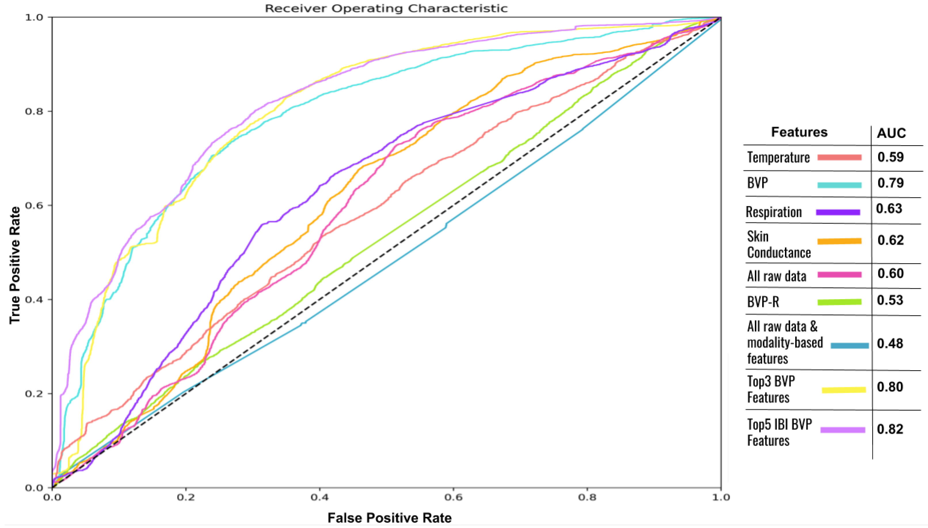
  • Receiver operating characteristic curve (ROC): ROC curve is a graphical way to visualize the classification ability of a binary classifier. ROC curves describe the relation between TP-rate and FP-rate at different thresholds. FP-rate is given as 1-specificity. The area under the ROC curve is equal to the probability that the model will classify a randomly chosen positive instance higher than a randomly chosen negative one. The area under the ROC curve, also known as AUC, is a measure of the general ability of the network to discriminate between the two classes. The higher the AUC, the better the model.

3.6. Normalization and Classification Setup

Due to limited available compute, to reduce the computational demands of the problem we sub-sample all available information streams to 8Hz. Then, the data of each participant are normalized based on their afternoon baseline recording (see Section 3.1). We choose afternoon baseline over the morning one, as it led to slightly better overall performance during experimentation. The normalization formula is shown in Equation (4).
x i , j ^ = x i , j m e a n ( x a f t e r n o o n _ b a s e l i n e ) s t d ( x a f t e r n o o n _ b a s e l i n e )
where x i , j ^ is the normalized feature value x i of feature x and j is the participant ID.
Finally, consecutive samples are grouped into batches of 64 by using an eight second, non-overlapping windowing approach. As a result, all of our models provide one prediction every 8 s. For all classification experiments, we apply a 10-fold cross validation scheme, using at each fold 20% of the users for testing and the rest of the users for training.

4. Single and Joint Task Learning

For our experiments we target two main conditions: drowsiness and distraction. For the former condition, data collected during the morning recording sessions are labeled as ‘alert’, while data collected during the afternoon recording session are marked as ‘drowsy’. This labeling was decided based on findings coming from related research conducted over the years [5,35,36,37,38]. For the latter, data corresponding to any of the distraction segments are labeled as ’distracted’, while data collected under the free-driving part are labeled as ‘not-distracted’.

4.1. Single Task Learning

For our single-task learning experiments, we investigate four different classification techniques. In particular, three traditional machine learning classifiers are being tested as well as a deep-learning pipeline that is known for its effectiveness on learning spatio-temporal representations. All three standard machine learning models have been extensively applied in the related literature for physiological signal classification tasks and for driver monitoring in particular, while the deep structure has been evaluated on various temporal modeling tasks for single-modality and multimodal representation learning. More specifically, the following classifiers are being tested:
  • An SVM classifier using an RBF Kernel [44,45,46].
  • A Nearest Neighbor classifier with K = 7 [47,48,49].
  • A Random Forest (RF) model with 100 estimators [50,51,52].
  • A CNN-LSTM pipeline. The evaluated deep architecture was initially proposed by Donahue et al. in 2015 for video captioning and since then has been evaluated on several tasks that are based on physiological signal monitoring [53,54] mostly related to the medical domain. Only quite recently was the method also applied for the problem of multimodal stress monitoring in drivers [30]. The general model structure is shown in Figure 2. Our model, consists of two convolutional layers with 64 filters of size five, followed by an LSTM unit with a memory of 64. At the end, a fully connected layer of size 64 with a softmax activation for classification is applied. After each convolutional layer a 20% dropout is performed. The model is optimized based on categorical cross-entropy using an Adam optimizer [55]. All the hyper-parameters of the model, including the number and size of the different layers, were tuned after experimentation and through an exhaustive grid search evaluation of different parameter-value combinations. The proposed method performs practically two levels of temporal modeling on the input data. First, the CNN takes as input windows of 64 × n u m b e r _ o f _ f e a t u r e s corresponding to data captured over a period of 8 s. Then, the LSTM unit accounts for the sequence of incoming frames taking into account data captured over approximately the past 8.5 min (given that it has a memory of 64). This design provides the model with great temporal depth that allows it to better account for future changes in behavior.

4.2. Joint-Task Learning

For joint modeling of alertness and distraction, we evaluate four different deep-learning schemes. All four architectures are shown in Figure 3 and are inspired by the original deep model shown in Figure 2.
  • Scheme A—Figure 3a: This model consists of two parallel networks, where each branch is dedicated to a specific task. Both branches are copies of the network shown in Figure 3. No layers are shared across the two tasks, but the two branches are trained using the same optimization function, which is estimated as the sum of task-based cross entropies. For getting a classification probability for each task a softmax function is applied at the dense layer of each branch.
  • Scheme B—Figure 3b: This approach also formulates the problem as a multitask learning process. The difference compared to Scheme A is that both the convolutional and the LSTM layers are shared across the two tasks. After the LSTM unit, the network splits again into two branches with a dense layer dedicated explicitly on an individual task. As before the two tasks are optimized based on the average task-based cross entropies and a softmax function is used to estimate the probability of the assigned label at each branch.
  • Scheme C—Figure 3c: In this approach we train a single network on a multilabel classification task. All layers are shared and a vector of size two is being predicted at the end, where each element corresponds to a task-specific label. The predicted vector values are estimated based on two sigmoid functions, each one dedicated to a specific task. In this case, all layers are shared across the two tasks and no task-based tailoring is being applied.
  • Scheme D—Figure 3d: The last model formulates the problem as a single task multi-class classification process. In this case we have four labels, where each of them describes a unique combination of distracted and drowsy states. In particularly the four labels are: drowsy and distracted, drowsy and not-distracted, alert and distracted and alert and not-distracted. This formulation was inspired by the approach initially proposed by Riani et al. [26] where the authors did the same thing using a DT classifier.
Similarly to the single-task CNN-LSTM models, all the joint-task models are trained based on the categorical cross entropy along with an Adam optimizer.

5. Results

We perform three types of experiments. Initially we show our results on drowsiness detection by measuring on different feature sets using the CNN-LSTM pipeline. In, addition, we compare the best performing CNN-LSTM model against the three traditional ML classifiers (Section 4.1). Then, we apply the same evaluation for the distraction detection task. At last, we explore how the different joint modeling approaches (Section 4.2) perform in detecting driver drowsiness and distraction in parallel and we compare their performance against the more traditional modeling alternatives.

5.1. Single-Task Learning

Firstly we perform a general evaluation across different feature combinations using the deep CNN-LSTM pipeline. The results for drowsiness and distraction detection are presented in Figure 4 and Figure 5, respectively, in terms of ROC curves and AUC score. Then, for the best feature set at each task we evaluate all classifiers in terms of sensitivity, specificity and average recall and we discuss the contribution of different features and models to identify the two conditions.
In particular, the following feature combinations are being presented:
  • BVP: Raw BVP data plus 49 temporal features extracted from the BVP signal.
  • Respiration: Raw respiration data plus eight temporal features extracted from the respiration signal.
  • Skin conductance: Raw skin conductance data plus six temporal features extracted from the skin conductance signal.
  • Temperature: Raw skin temperature data plus six temporal features extracted from the skin temperature signal.
  • All raw data and modality-based features: The input data consist of the concatenation of all features and raw signals mentioned above.
  • All raw data: Only the raw data from the four physiological sources are concatenated and used as input features.
  • BVP + respiration (BVP-R): We evaluated different combinations of raw data as input features. Out of all the possible mixtures, combining BVP and respiration data stood out as the most efficient combination for part of our experiments.
  • Top #5 BVP features: The input data consist of the top #5 (Table 2) performing features as identified through the analysis discussed in Section 3.4.
  • Top #3 IBI BVP features: The input data consist of the top #3 BVP features that are related to IBI (features #1, #2 and #5 of Table 2).

5.2. Drowsy Driver Modeling

For this experiments we split the data into the two following classes; recordings made during the morning session (8 a.m. to 11 a.m.) are labeled as ‘alert’, while recordings made during the afternoon session (4 p.m. to 8 p.m.) are marked as ‘drowsy’. We perform a 10-fold cross validation across the participants using 20% of the users for testing and the rest 80% for training.
As shown in Figure 4 from all the evaluated feature sets, the combination of “BVP and respiration” signals is by far the most efficient approach, achieving an AUC performance of 88%. These results are partially in line with the findings presented in Section 3.4, which identified that specific BVP statistics are highly related to both tasks. On the other hand, in contrast to the features identified through the analysis of Section 3.4, we observe that respiration related data are also highly associated with drowsiness. In particular, the “top3 IBI BVP features” set along with all the “respiration related data” are responsible for the second and third best AUC scores with 75% and 74%, respectively. However, when we combine all BVP features, the performance drops significantly to 61%. We believe that the significant increase in feature space along with the decrease in available data after sub-sampling the signals to 8Hz is partially responsible for that observation, since the network parameters do not have access to the required amount of information in order to get properly trained. In addition, it is highly possible that several BVP features are not actually good descriptors of drowsiness, thus adding noise to the input instead of actually assisting to the final decision. On the other hand, it seems that just joining the two raw information streams of BVP and respiration is sufficient for the network to capture the important characteristics of the signals. We believe that this could potentially relate to the fact that both signals have a periodic behavior and we know for a fact that characteristics related to IBIs for the BVP signal and to rate and amplitude for the respiration signal, are of special importance to the task. This can be confirmed by the high performance observed when using explicitly the top3 IBI BVP features or the set of respiration related data accordingly. The rest of the evaluated feature combinations do not offer any significant value on this task showing performance that is comparable to random guess.
Focusing on the results of Table 3, we see that the CNN-LSTM model performs significantly better compared to all the baseline classifiers when trained only on the raw BPV and respiration data. The very poor performance of the baseline classifiers is indicative of how challenging the targeted problem is, while at the same time highlights the superiority of the deep spatio-temporal classifier compared to the traditional and more popular alternatives on the task of physiological-based drowsy driver behavior modeling. In particular, all baseline classifiers perform very poorly in terms of sensitivity with very high specificity scores. In other words, these models fail marginally to identify drowsy behavior. However, it is very unlikely to identify someone who is actually alert as drowsy. On the contrary, the CNN-LSTM model outperforms by far all baselines in terms of sensitivity with a score of 93%, while it provides worse but reasonable results in terms of specificity with a score of 71%. This means that the chance of correctly identifying drowsy behavior with this model is quite high, even though in approximately three out of ten times an alert driver will be wrongfully identified as drowsy.

5.3. Distracted Driver Modeling

For this experiment we split the data as follows; data corresponding to any of the distraction segments is labeled as ‘distracted’, while data collected under the free-driving part is labeled as ‘not-distracted’. To minimize the biases introduced by the relatively unfamiliar virtual-driving setup, we use five minute long data segments, extracted from the last seven minutes of the free-driving recording, when subjects were already used to the driving simulator.
Similarly to the previous section, we perform a feature based analysis using the deep CNN-LSTM model. By observing the ROC curves of Figure 5 it would be safe to assume that identifying distracted behavior based on the selected feature-sets is relatively more challenging compared to detecting drowsiness. According to the AUC scores, all BVP related feature combinations provide by far the best results, indicating the strong relation of heart-rate related features to the task. More specifically, best results were achieved by the “top5 BVP” features of Table 2, with an AUC of 82% while second comes the “top3 IBI BVP” feature set with an AUC of 80% and third the set with “all BVP” related data with an AUC score of 79%. Of special interest is the very poor performance observed by the combination of raw BVP and respiration data, which provided the best results in the problem of drowsiness detection. Even though it is hard to clearly explain the very low performance of this feature set, we suspect that the overall poor performance of the respiration data on the task affects the results in a negative way. Judging from the AUC score achieved by the “respiration” feature set it seems that respiratory data are not as related to distracted behavior as they are to the drowsy one. However, these negative results need to be further evaluated in the future.
Taking these findings into consideration, we evaluate the different classifiers on their ability to identify distracted driving based on the “top5 BVP” feature set. The results are presented in Table 4. Again, the CNN-LSTM model significantly outperforms all three baselines. The model provides the most balanced results with an average recall of 72%. The advantage of the CNN-LSTM model against its competitors, is less on its ability to identify distracted behavior and more on its balanced performance between sensitivity and specificity. In particular, the SVM model performs better on identifying non-distracted driving while its predictive ability with respect to distraction detection is almost random, thus making this approach the less appropriate of all for the purposes of the task. On the other hand, KNN and RF classifiers perform equally to the CNN-LSTM model on identifying drowsy driving. However, their high FP-rate makes them less appropriate for modeling the problem as they have almost a 50% chance on marking a not-distracted driver as distracted.
Overall, we can argue that the CNN-LSTM pipeline is by far the most effective on modeling both distracted and drowsy driver states, under the same experimentation conditions. That is both in terms of correctly identifying the condition of interest (more TPs) but also in discriminating against it (more TNs).

5.4. Multitask Learning for Joint Driving Behavior Modeling

Dedicating a single machine learning model to each condition of interest has been traditionally the most popular and effective approach of dealing with problems related to human behavior modeling. However, in several cases we are interested in predicting conditions that coexists and may overlap. Our assumption is that overlapping conditions may share a common ground in terms of physiological reactions caused to the drivers. To that end we evaluate different machine learning methods on their ability to jointly predict driver’s state in terms of distraction and alertness. For these experiments we use the combination of the seven temporal features that performed the best for the individual tasks. Hence, each training feature vector consists of the raw recordings from BVP and respiration plus the five BVP features identified through the analysis of Section 3.4.
Figure 3 illustrates all the deep learning methods evaluated. For the cases of SVM, RF and KNN we formulate the problem similarly to the deep Scheme D model, i.e., as a 4-class classification task.
In order to have a fair comparison against the different approaches, we evaluate all models on their ability to correctly identify drowsiness and distraction as independent tasks. In the case of multi-class models (ScemeD, SVM, KNN, RF) in particular, the results are evaluated as two binary classification problems and not as a traditional four-class task. Formulating evaluation as such, allows for a one to one comparison against the multitask methods (Shemes A, B, C) and avoids diluting the characterization ability of the different classifiers with respect to the individual conditions, while still learning shared parameters between tasks.
Figure 6 shows the ROC curves for all the deep learning-based models for both tasks. Solid lines correspond to the drowsiness detection task, while dotted lines to distraction detection. Schemes A and B offer the most balanced results across the two detection problems. In particular, the two models perform comparably well to the CNN-LSTM distraction model (Figure 5), while providing the second and third best results for the drowsiness task in terms of AUC when compared to the alternatives of Figure 4. However, despite the fact that the performance is acceptable for both tasks, it always remains inferior to the condition-targeted classifiers. This could be partially an effect related to the limited amount of data available to properly tune the model parameters. Another possible explanation could be that other than the IBI BVP features that have a proven value on characterizing both conditions, the rest of the input features are less robust across tasks, thus hindering the model’s ability to converge at a higher overall score.
Nonetheless, it is clear that Schemes A and B offer overall the best modeling performance across all the approaches that jointly learn representations for the two conditions. These architectures are the only ones that have dedicated layers for each task, while their parameters are being updated based on an optimization error that takes into account both individual performances. Based on these results, we can see that the number of shared layers does not have a significant impact on the task-specific performance, even though this might change as the available training data increase. Scheme C, which has all layers shared across the two tasks, performs the worst in terms of AUC. This observation to some extend indicates the fact that the physiological responses caused by the two conditions are not the same but are overlapping to some extend given that the model achieves a a performance significantly higher than random for both conditions. At last, Scheme D, which is the multi-class approach, slightly underperforms compared to the branched, multitask learning approaches. The model also exploits the shared layers across tasks to learn parameters of importance related to both conditions. At the same time, the discrimination into four classes assists the model to learn how the different physiological responses relate to the presence or absence of each of the conditions simultaneously. However, splitting the data into four classes limits the available data under each category thus, having a negative impact on models performance.
Table 5 shows in more detail the performance of all the classifiers in terms of sensitivity, specificity and average recall. All deep learning based methods perform significantly better compared to the traditional machine learning models both in single-task and joint-task evaluations (see also Table 3 and Table 4). At the same time, Schemes A and B, which are the two multitask learning approaches with a branching architecture, provide the best results in terms of average recall. That is due to the fact that the two models offer the best trade-off between sensitivity and specificity for the detection of both conditions. Of special interest is the high performance observed by Scheme C in terms of sensitivity. The model offers higher scores than all joint-learning alternatives for the drowsiness detection task, while it outperforms by far all methods tested on the distraction detection task. That means that in terms of detecting the conditions of interest Scheme C is the most effective one. However, its poor performance in terms of specificity makes it an inappropriate model to be applied in a real life scenario, since the high rate of false alarms would lead to an over-sensitive monitoring system.

6. Conclusions

In this paper, we explore different physiological markers and machine learning approaches on their ability to describe distracted and drowsy driving. For our analysis, we compiled a dataset of 45 subjects and we recorded their BVP, respiration, skin conductance and skin temperature responses while participating in a simulated driving setup. Based on our analysis, the contribution of this publication can be summarized through the answers on the following three research questions:
  • Which physiological indicators are most indicative of drowsy and distracted behavior?
With respect to drowsiness detection, BVP and respiration indicators proved to be the two signals that are mostly associated with the task. In particular, the combination of the raw BVP and respiration measurements leads to maximum drowsiness detection performance in terms of AUC score with a value of 88%, when processed through a spatio-temporal deep CNN-LSTM model. Second best performance, with a score of 75% AUC, is achieved by a subset of BVP related features when processed through the same modeling architecture, while respiration related data and features, lead to the third best performance with a score of 74% AUC. Skin conductance and temperature signals and features lead to significantly inferior performance, with their AUC scores fluctuating around 50%.
With regard to distraction detection, BVP proved to be again highly associated with the task. All feature sets extracted from that signal marginally outperform all the alternative feature combinations when processed through the same spatio-temporal CNN-LSTM architecture, by achieving AUC scores in the range between 79% to 82%. The rest of the evaluated feature sets, which consist of various combinations of the remaining physiological markers and their statistical features, always perform around 60% AUC. Hence, showing their relation to distracted behavior but also highlighting their weakness on robustly capturing the condition when used exclusively.
  • Are there specific statistical features coming from different signals that are particularly informative?
Our analysis discussed in Section 3.4 and further evaluated in Section 5.2 and Section 5.3, identified several features of importance related to the two conditions.
More specifically, we train two DT classifiers targeted on the individual tasks, using all the available data, and we perform an entropy-based evaluation of all the available features on their importance towards detecting the two conditions. Figure A1 in the Appendix A illustrates the importance of all features in terms of information gain after training the two models. Based on this analysis, we select the five most informative statistical features, presented in Table 2. As it can be observed, all five features are related to BVP and in particular three are extracted from the time domain and describe patterns related to BVP IBIs and two are extracted from the spectral domain and are related to the spectral power of the signal in different frequency bands. BVP IBI related statistics alone show great performance on both tasks as they lead to the second best performance in both drowsiness detection with 75% AUC and distraction detection with 80% AUC. Interestingly, when combined with the frequency related features, the new feature set performs quite poorly on the drowsiness detection task leading to almost random performance with 50% AUC while it offers the best results on drowsiness detection with 82% AUC. It is not clear yet why adding the frequency features to the input feature set harms the classifier so abruptly with respect to drowsiness detection and this is something that we would like to investigate further in the future.
In addition to the BVP features, respiration related statistics showed strong association with drowsy driving. In particular, combining the raw respiration data with temporal features describing the temporal characteristics of the signal leads to a 74% AUC, which is the third highest score achieved by the single-task deep model for drowsiness detection. Specifically the features extracted from respiration correspond to: respiration amplitude, respiration period, respiration rate, respiration rate epoch mean (where an epoch is 5 min of data), respiration rate mean (br/min) and respiration rate std dev (br/min).
  • Is it possible to jointly tackle the problems of drowsiness and distraction detection and how such a framework can be formulated?
Overall, our experiments showed that deep CNN-LSTM-based methods significantly outperform all other evaluated traditional machine learning alternatives, which have the lion’s share in evaluations presented in the related literature (RFs, KNN, SVM). In particular, the single-task CNN-LSTM model leads to a maximum performance of 88% AUC with 82% average recall for the drowsiness detection task and to 82% AUC with 72% average recall for the distraction detection task. Second best performance however across both tasks, is recorded by the joint condition learning multitask schemes with a branching architecture (Schemes A and B of Figure 3). Our evaluations highlight the potential of multitask learning towards directly addressing such abstract conditions with overlapping physiological responses. Schemes A and B offer results directly comparable to the corresponding single-task CNN-LSTM model for the distraction detection task with ~79.5% AUC and a slightly improved 73% average recall. At the same time, for the drowsiness detection task the models achieve a ~76.5% AUC and 72.5% average recall. Even though performance is lower in terms of AUC and sensitivity compared to the single-task CNN-LSTM model in the case of drowsiness detection, the classifier still performs notably higher compared to all other evaluated methods on the task.
In general, we argue that building multitask learning models with dedicated layers on every targeted task is the method that showed the most promising results, on joint condition learning. Avoiding branching and having only shared layers across tasks led to the worst results as the model struggled to effectively distinguish between conditions, since the learned features could not scale equally across tasks. The multi-class approach also offered inferior results compared to multitask learning as the division of training data into multiple groups had a negative impact on the final result.
Even though condition-specific models still offer the optimal results, our findings strongly indicate that joint condition modeling using multitask learning has great future potential on this and similar tasks and we plan to investigate this direction further in the near future. In addition, a limitation of the current analysis is that the levels of drowsiness experienced by the participants are not practically measurable. Our assumption about drowsiness is derived mostly by previous highly credible research (including NHTSA findings [5]) and the daily schedule of our specific target group (young adults who are graduate and undergraduate university students). In future versions of the dataset, we plan to introduce additional drowsiness evaluation methods such as subjective sleepiness reporting [56] and objective test-based evaluations [57] to better quantify and measure the presence of drowsiness in our recordings.

Author Contributions

M.P. lead the research of this work by guiding, designing and implementing all the experimental procedures described in the paper and by writing the manuscript. K.D. assisted on the experimental design and developed most of the code needed for the discussed experiments in collaboration with M.P., M.A., R.M. and M.B. assisted with advising, mentoring and supervision and also with securing the funds and resources needed for this research. All authors have read and agreed to the published version of the manuscript.

Funding

This material is based in part upon work supported by the Toyota Research Institute (“TRI”). Any opinions, findings, and conclusions or recommendations expressed in this material are those of the authors and do not necessarily reflect the views of TRI or any other Toyota entity.

Institutional Review Board Statement

The study was conducted according to the guidelines of the Declaration of Helsinki, and approved by the Institutional Review Board of University of Michigan, Ann Arbor under the identification code HUM00132603 on 31 October 2018.

Informed Consent Statement

Informed consent was obtained from all subjects involved in the study.

Data Availability Statement

Please refer to suggested Data Availability Statements in section “MDPI Research Data Policies” at https://0-www-mdpi-com.brum.beds.ac.uk/ethics.

Conflicts of Interest

The authors declare no conflict of interest.

Abbreviations

The following abbreviations are used in this manuscript:
AUCarea under curve
BPMbeats per minute
BRbreathing rate
BVPblood volume pulse
CNNconvolutional neural network
DTdecision tree
FNfalse negatives
FPfalse positives
LSTMlong short-term memory
ECGelectrocardiogram
EEGelectroencephalogram
EMGelectromyogram
GSRgalvanic skin response
IBIinter-beat intervals
KNNK nearest neighbors
RFrandom forest
ROCreceiver operating characteristic
SVMsupport vector machine
TNtrue negatives
TPtrue positives
WHOWorld Health Organization

Appendix A

Figure A1. An epoch corresponds to 5 min of data.
Applsci 11 00088 g0a1

References

  1. Wang, Y.; Zhang, D.; Liu, Y.; Dai, B.; Lee, L.H. Enhancing transportation systems via deep learning: A survey. Transportation Research Part C: Emerging Technologies. 2019, 99, 144–163. [Google Scholar] [CrossRef]
  2. World Health Organisation. Mobile Phone Use: A Growing Problem Of Driver Distraction. 2011. Available online: https://www.who.int/violence_injury_prevention/publications/road_traffic/distracted_driving_en.pdf?ua=1 (accessed on 19 October 2020).
  3. World Health Organisation. Road Traffic Injuries. 2020. Available online: https://www.who.int/news-room/fact-sheets/detail/road-traffic-injuries (accessed on 19 October 2020).
  4. National Highway Traffic Safety Administration (NHTSA), US Department of Transportation. 2019; Distracted Driving. Available online: https://www.nhtsa.gov/risky-driving/distracted-driving (accessed on 19 October 2020).
  5. National Highway Traffic Safety Administration (NHTSA), US Department of Transportation. 2018; Drowsy Driving. Available online: https://www.nhtsa.gov/risky-driving/drowsy-driving (accessed on 19 October 2020).
  6. Sigari, M.H.; Fathy, M.; Soryani, M. A driver face monitoring system for fatigue and distraction detection. Int. J. Veh. Technol. 2013, 5, 73–100. [Google Scholar] [CrossRef] [Green Version]
  7. Kutila, M.; Jokela, M.; Markkula, G.; Rué, M.R. Driver distraction detection with a camera vision system. In Proceedings of the 2007 IEEE International Conference on Image Processing, San Antonio, TX, USA, 16–19 September 2007; IEEE: Piscataway, NJ, USA, 2007; Voume 6, p. VI-201. [Google Scholar]
  8. Yang, D.; Li, X.; Dai, X.; Zhang, R.; Qi, L.; Zhang, W.; Jiang, Z. All In One Network for Driver Attention Monitoring. In Proceedings of the ICASSP 2020-2020 IEEE International Conference on Acoustics, Speech and Signal Processing (ICASSP), Barcelona, Spain, 4–8 May 2020; IEEE: Piscataway, NJ, USA, 2020; pp. 2258–2262. [Google Scholar]
  9. Harbluk, J.L.; Noy, Y.I.; Trbovich, P.L.; Eizenman, M. An on-road assessment of cognitive distraction: Impacts on drivers’ visual behavior and braking performance. Accid. Anal. Prev. 2007, 39, 372–379. [Google Scholar] [CrossRef]
  10. Savelonas, M.; Karkanis, S.; Spyrou, E. Classification of Driving Behaviour using Short-term and Long-term Summaries of Sensor Data. In Proceedings of the 2020 5th South-East Europe Design Automation, Computer Engineering, Computer Networks and Social Media Conference (SEEDA-CECNSM), Corfu, Greece, 25–27 September 2020; IEEE: Piscataway, NJ, USA, 2020; pp. 1–4. [Google Scholar]
  11. Xie, Y.; Murphey, Y.L.; Kochhar, D. Personalized Driver Workload Estimation Using Deep Neural Network Learning from Physiological and Vehicle Signals. IEEE Trans. Intell. Veh. 2019. [Google Scholar] [CrossRef]
  12. Healey, J.A.; Picard, R.W. Detecting stress during real-world driving tasks using physiological sensors. IEEE Trans. Intell. Transp. Syst. 2005, 6, 156–166. [Google Scholar] [CrossRef] [Green Version]
  13. Singh, R.R.; Conjeti, S.; Banerjee, R. A comparative evaluation of neural network classifiers for stress level analysis of automotive drivers using physiological signals. Biomed. Signal Process. Control 2013, 8, 740–754. [Google Scholar] [CrossRef]
  14. Wang, K.; Guo, P. An Ensemble Classification Model With Unsupervised Representation Learning for Driving Stress Recognition Using Physiological Signals. IEEE Trans. Intell. Transp. Syst. 2020. [Google Scholar] [CrossRef]
  15. Desmond, P.A.; Matthews, G. Individual differences in stress and fatigue in two field studies of driving. Transp. Res. Part F Traffic Psychol. Behav. 2009, 12, 265–276. [Google Scholar] [CrossRef]
  16. Brookhuis, K.A.; De Waard, D. Monitoring drivers’ mental workload in driving simulators using physiological measures. Accid. Anal. Prev. 2010, 42, 898–903. [Google Scholar] [CrossRef]
  17. Reimer, B.; Mehler, B. The impact of cognitive workload on physiological arousal in young adult drivers: A field study and simulation validation. Ergonomics 2011, 54, 932–942. [Google Scholar] [CrossRef]
  18. Zhang, L.; Wade, J.; Bian, D.; Fan, J.; Swanson, A.; Weitlauf, A.; Warren, Z.; Sarkar, N. Cognitive load measurement in a virtual reality-based driving system for autism intervention. IEEE Trans. Affect. Comput. 2017, 8, 176–189. [Google Scholar] [CrossRef] [PubMed]
  19. Nourbakhsh, N.; Chen, F.; Wang, Y.; Calvo, R.A. Detecting users’ cognitive load by galvanic skin response with affective interference. ACM Trans. Interact. Intell. Syst. TiiS 2017, 7, 1–20. [Google Scholar] [CrossRef] [Green Version]
  20. Schmidt, M.; Bhandare, O.; Prabhune, A.; minker, W.; Werner, S. Classifying Cognitive Load for a Proactive In-car Voice Assistant. In Proceedings of the 2020 IEEE Sixth International Conference on Big Data Computing Service and Applications (BigDataService), Oxford, UK, 3–6 August 2020; IEEE: Piscataway, NJ, USA, 2020; pp. 9–16. [Google Scholar]
  21. Awais, M.; Badruddin, N.; Drieberg, M. A hybrid approach to detect driver drowsiness utilizing physiological signals to improve system performance and wearability. Sensors 2017, 17, 1991. [Google Scholar] [CrossRef] [PubMed] [Green Version]
  22. Persson, A.; Jonasson, H.; Fredriksson, I.; Wiklund, U.; Ahlström, C. Heart Rate Variability for Driver Sleepiness Classification in Real Road Driving Conditions. In Proceedings of the 2019 41st Annual International Conference of the IEEE Engineering in Medicine and Biology Society (EMBC), Berlin, Germany, 23–27 July 2019; IEEE: Piscataway, NJ, USA, 2019; pp. 6537–6540. [Google Scholar]
  23. Sahayadhas, A.; Sundaraj, K.; Murugappan, M.; Palaniappan, R. A physiological measures-based method for detecting inattention in drivers using machine learning approach. Biocybern. Biomed. Eng. 2015, 35, 198–205. [Google Scholar] [CrossRef]
  24. Taherisadr, M.; Asnani, P.; Galster, S.; Dehzangi, O. ECG-based driver inattention identification during naturalistic driving using Mel-frequency cepstrum 2-D transform and convolutional neural networks. Smart Health 2018, 9, 50–61. [Google Scholar] [CrossRef]
  25. Dehzangi, O.; Sahu, V.; Rajendra, V.; Taherisadr, M. GSR-based distracted driving identification using discrete & continuous decomposition and wavelet packet transform. Smart Health 2019, 14, 100085. [Google Scholar]
  26. Riani, K.; Papakostas, M.; Kokash, H.; Abouelenien, M.; Burzo, M.; Mihalcea, R. Towards detecting levels of alertness in drivers using multiple modalities. In Proceedings of the 13th ACM International Conference on PErvasive Technologies Related to Assistive Environments, Corfu, Greece, June 2020; pp. 1–9. [Google Scholar]
  27. Lim, S.; Yang, J.H. Driver state estimation by convolutional neural network using multimodal sensor data. Electron. Lett. 2016, 52, 1495–1497. [Google Scholar] [CrossRef] [Green Version]
  28. Zeng, H.; Yang, C.; Dai, G.; Qin, F.; Zhang, J.; Kong, W. EEG classification of driver mental states by deep learning. Cogn. Neurodynamics 2018, 12, 597–606. [Google Scholar] [CrossRef]
  29. Choi, H.T.; Back, M.K.; Lee, K.C. Driver drowsiness detection based on multimodal using fusion of visual-feature and bio-signal. In Proceedings of the 2018 International Conference on Information and Communication Technology Convergence (ICTC), Jeju Island, Korea, 17–19 October 2018; IEEE: Piscataway, NJ, USA, 2018; pp. 1249–1251. [Google Scholar]
  30. Rastgoo, M.N.; Nakisa, B.; Maire, F.; Rakotonirainy, A.; Chandran, V. Automatic driver stress level classification using multimodal deep learning. Expert Syst. Appl. 2019, 138, 112793. [Google Scholar] [CrossRef]
  31. Gjoreski, M.; Gams, M.Ž.; Luštrek, M.; Genc, P.; Garbas, J.U.; Hassan, T. Machine Learning and End-to-End Deep Learning for Monitoring Driver Distractions From Physiological and Visual Signals. IEEE Access 2020, 8, 70590–70603. [Google Scholar] [CrossRef]
  32. Craye, C.; Rashwan, A.; Kamel, M.S.; Karray, F. A multi-modal driver fatigue and distraction assessment system. Int. J. Intell. Transp. Syst. Res. 2016, 14, 173–194. [Google Scholar] [CrossRef]
  33. Choi, M.; Koo, G.; Seo, M.; Kim, S.W. Wearable device-based system to monitor a driver’s stress, fatigue, and drowsiness. IEEE Trans. Instrum. Meas. 2017, 67, 634–645. [Google Scholar] [CrossRef]
  34. Sarkar, P.; Ross, K.; Ruberto, A.J.; Rodenbura, D.; Hungler, P.; Etemad, A. Classification of cognitive load and expertise for adaptive simulation using deep multitask learning. In Proceedings of the 2019 8th International Conference on Affective Computing and Intelligent Interaction (ACII), Cambridge, UK, 3–6 September 2019; IEEE: Piscataway, NJ, USA, 2019; pp. 1–7. [Google Scholar]
  35. National Heart, Lung, and Blood Institute and National Highway Traffic Safety Administration (NHTSA). Drowsy Driving and Automobile Crashes. 1998. Available online: https://rosap.ntl.bts.gov/view/dot/1661 (accessed on 7 December 2020).
  36. Beirness, D.J.; Herb, M.; Desmond, K. The road safety monitor 2004: Drowsy driving. In The 2004 Annual Public Opinion Survey by the Traffic Injury Research Foundation; Traffic Injury Research Foundation (TIRF): Ottowa, ON, Canada.
  37. Caponecchia, C.J.; Williamson, A. Drowsiness and driving performance on commuter trips. J. Saf. Res. 2018, 66, 179–186. [Google Scholar] [CrossRef] [PubMed]
  38. Guede, F.; Chimeno, M.; Castro, J.; Gonzalez, M. Driver drowsiness detection based on respiratory signal analysis. IEEE Access 2019, 7, 81826–81838. [Google Scholar] [CrossRef]
  39. Kane, M.J.; Conway, A.R.; Miura, T.K.; Colflesh, G.J. Working memory, attention control, and the N-back task: A question of construct validity. J. Exp. Psychol. Learn. Mem. Cogn. 2007, 33, 615. [Google Scholar] [CrossRef] [PubMed] [Green Version]
  40. Karthikeyan, P.; Murugappan, M.; Yaacob, S. Descriptive analysis of skin temperature variability of sympathetic nervous system activity in stress. J. Phys. Ther. Sci. 2012, 24, 1341–1344. [Google Scholar] [CrossRef] [Green Version]
  41. Mackersie, C.L.; Calderon-Moultrie, N. Autonomic nervous system reactivity during speech repetition tasks: Heart rate variability and skin conductance. Ear Hear. 2016, 37, 118S–125S. [Google Scholar] [CrossRef]
  42. Storm, H.; Myre, K.; Rostrup, M.; Stokland, O.; Lien, M.; Raeder, J. Skin conductance correlates with perioperative stress. Acta Anaesthesiol. Scand. 2002, 46, 887–895. [Google Scholar] [CrossRef] [Green Version]
  43. Malik, M.; Bigger, J.T.; Camm, A.J.; Kleiger, R.E.; Malliani, A.; Moss, A.J.; Schwartz, P.J. Heart rate variability: Standards of measurement, physiological interpretation, and clinical use. Eur. Heart J. 1996, 17, 354–381. [Google Scholar] [CrossRef] [Green Version]
  44. Hearst, M.A.; Dumais, S.T.; Osuna, E.; Platt, J.; Scholkopf, B. Support vector machines. IEEE Intell. Syst. Their Appl. 1998, 13, 18–28. [Google Scholar] [CrossRef] [Green Version]
  45. Li, G.; Chung, W.Y. Detection of driver drowsiness using wavelet analysis of heart rate variability and a support vector machine classifier. Sensors 2013, 13, 16494–16511. [Google Scholar] [CrossRef] [PubMed] [Green Version]
  46. Chen, H.; Chen, L. Support vector machine classification of drunk driving behaviour. Int. J. Environ. Res. Public Health 2017, 14, 108. [Google Scholar] [CrossRef] [PubMed]
  47. Yakowitz, S. Nearest-neighbour methods for time series analysis. J. Time Ser. Anal. 1987, 8, 235–247. [Google Scholar] [CrossRef]
  48. Munla, N.; Khalil, M.; Shahin, A.; Mourad, A. Driver stress level detection using HRV analysis. In Proceedings of the 2015 international conference on advances in biomedical engineering (ICABME), Beirut, Lebanon, 16–18 September 2015; IEEE: Piscataway, NJ, USA, 2015; pp. 61–64. [Google Scholar]
  49. Wang, J.S.; Lin, C.W.; Yang, Y.T.C. A k-nearest-neighbor classifier with heart rate variability feature-based transformation algorithm for driving stress recognition. Neurocomputing 2013, 116, 136–143. [Google Scholar] [CrossRef]
  50. Liaw, A.; Wiener, M. Classification and regression by randomForest. R News 2002, 2, 18–22. [Google Scholar]
  51. Hassib, M.; Braun, M.; Pfleging, B.; Alt, F. Detecting and influencing driver emotions using psycho-physiological sensors and ambient light. In IFIP Conference on Human-Computer Interaction; Springer: Berlin/Heidelberg, Germany, 2019; pp. 721–742. [Google Scholar]
  52. Wang, M.; Jeong, N.; Kim, K.; Choi, S.; Yang, S.; You, S.; Lee, J.; Suh, M. Drowsy behavior detection based on driving information. Int. J. Automot. Technol. 2016, 17, 165–173. [Google Scholar] [CrossRef]
  53. Faust, O.; Hagiwara, Y.; Hong, T.J.; Lih, O.S.; Acharya, U.R. Deep learning for healthcare applications based on physiological signals: A review. Comput. Methods Programs Biomed. 2018, 161, 1–13. [Google Scholar] [CrossRef]
  54. Rim, B.; Sung, N.J.; Min, S.; Hong, M. Deep Learning in Physiological Signal Data: A Survey. Sensors 2020, 20, 969. [Google Scholar] [CrossRef] [Green Version]
  55. Kingma, D.P.; Ba, J. Adam: A method for stochastic optimization. arXiv 2014, arXiv:1412.6980. [Google Scholar]
  56. Shahid, A.; Wilkinson, K.; Marcu, S.; Shapiro, C. Karolinska sleepiness scale (KSS). In STOP, THAT and One Hundred Other Sleep Scales; Springer: New York, NY, USA, 2011; pp. 209–210. [Google Scholar]
  57. Basner, M.; Mollicone, D.; Dinges, D. Validity and sensitivity of a brief psychomotor vigilance test (PVT-B) to total and partial sleep deprivation. Acta Astronaut. 2011, 69, 949–959. [Google Scholar] [CrossRef] [Green Version]
Figure 1. The data collection setup.
Applsci 11 00088 g001
Figure 2. Deep learning architecture for single-task learning.
Applsci 11 00088 g002
Figure 3. Deep learning schemes for joint modeling of driver distraction and drowsiness. (a) Scheme A: Multitask learning with no shared layers. (b) Scheme B: Multitask learning with shared convolutional and LSTM layers. (c) Scheme C: Multitask learning using a fully shared network. (d) Scheme D: Single-task 4-class classification.
Applsci 11 00088 g003
Figure 4. Receiver operating characteristic (ROC) curves and area under the ROC curve (AUC) scores for different feature sets on the task of drowsiness detection using the CNN-LSTM network.
Applsci 11 00088 g004
Figure 5. ROC curves and AUC scores for different feature sets on the task of distraction detection using the CNN-LSTM network.
Applsci 11 00088 g005
Figure 6. ROC curves of the four deep joint-modeling methods evaluated in this paper. Solid lines correspond to drowsiness detection ROCs and dotted lines to distraction detection. Average AUC is the AUC achieved by each model across both detection tasks.
Applsci 11 00088 g006
Table 1. Total duration of available data under each recording segment. For each segment, approximately half of the data come from the morning recordings and half from the afternoon.
Recording Segment
Free-drivingTexting
Physical
NBack
Cognitive
Neutral
Radio
Cognitive
Emotional
GPS
Cognitive
Frustration
#Data
(hours)
∼7.4∼3.1∼2.2∼3.4∼2
Table 2. Top five features based on increase of information gain when training a Random Forest classifier.
FeatureDescription
#1BVP IBI pNN Intervals (%)the percentage of successive intervals that differ by more than 50 ms
#2BVP IBI pNN Intervalsthe number of successive intervals that differ by more than 50 ms
#3BVP HF % power meanthe mean of power in the high frequencies
#4BVP LF % power meanthe mean of power in the low frequencies
#5BVP IBI NN Intervalsinterval between two normal heartbeats
Table 3. Alert vs. drowsy classification using the combination of raw blood volume pulse (BVP) and respiration data as selected by the analysis in Figure 4.
Drowsiness Detection
SVMKNNRFCNN-LSTM
Sensitivity (%)0171793
Specificity (%)92919171
Average Recall (%)46545482
Table 4. Distracted vs. not-distracted classification using the top5 BVP features as selected by the analysis in Figure 5 and Table 2.
Distraction Detection
SVMKNNRFCNN-LSTM
Sensitivity (%)53697070
Specificity (%)72525074
Average Recall (%)62.560.56072
Table 5. Task-based performance on joint condition learning of drowsiness and distraction.
Joint Condition Learning
SVMKNNRFScheme AScheme BScheme CScheme D
Drowsiness DetectionSensitivity (%)45252477738269
Specificity (%)64789168723763
Average Recall (%)54.551.557.572.572.559.566
Distraction DetectionSensitivity (%)51587075788478
Specificity (%)73525071685666
Average Recall (%)62556073737072
Publisher’s Note: MDPI stays neutral with regard to jurisdictional claims in published maps and institutional affiliations.

