Numerical Modeling of Temperature Effect on Tensile Strength of Granitic Rock

Abstract

The aim of this paper is to numerically predict the temperature effect on the tensile strength of granitic rock. To this end, a numerical approach based on the embedded discontinuity finite elements is developed. The underlying thermo-mechanical problem is solved with a staggered method marching explicitly in time while using extreme mass scaling, allowed by the quasi-static nature of the slow heating of a rock sample to a uniform target temperature, to increase the critical time step. Linear triangle elements are used to implement the embedded discontinuity kinematics with two intersecting cracks in a single element. It is assumed that the quartz mineral, with its strong and anomalous temperature dependence upon approaching the α-β transition at the Curie point (~573 °C), in granitic rock is the major factor resulting in thermal cracking and the consequent degradation of tensile strength. Accordingly, only the thermal expansion coefficient of quartz depends on temperature in the present approach. Moreover, numerically, the rock is taken as isotropic except for the tensile strength, which is unique for each mineral in a rock. In the numerical simulations mimicking the experimental setup on granitic numerical rock samples consisting of quartz, feldspar and biotite minerals, the sample is first heated slowly to a target temperature below the Curie point. Then, a uniaxial tension test is numerically performed on the cooled down sample. The simulations demonstrate the validity of the proposed approach as the experimental deterioration of the tensile strength of the rock is predicted with agreeable accuracy.

1. Introduction

Rocks often face high temperature conditions and thermal shocks in geotechnical engineering applications, such as harvesting deep geothermal energy [1], nuclear waste disposal [2], and thermal drilling [3]. Quartz-bearing rocks are particularly susceptible to temperature effects in their material properties and, consequently, in their response under thermal loading due to the α-β transition of quartz at its Curie point (~573 °C) [4]. Naturally, the temperature effects on rock mechanical properties have been extensively studied, experimentally [1,5,6,7,8,9,10,11,12,13,14] and numerically [11,12,13,14,15,16,17].

The temperature effects in rocks manifest as a degradation of mechanical properties (Young’s modulus and strength), while thermal properties show mixed behavior, i.e., some increase (thermal expansion coefficient, specific heat) while others decrease (thermal conductance) [7,11]. The degradation of mechanical properties, especially that of the tensile strength, is the most important aspect from a geotechnical engineering point of view. The main mechanism behind the deterioration of mechanical properties, i.e., damage, is thermal cracking due the pronounced heterogeneity of a rock material [13]. More precisely, a mismatch in the elastic properties leads to thermal stresses at mineral grain boundaries, which causes intra- and intergranular cracking, even under a uniform temperature field. With quartz-bearing rocks, such as granite, this heterogeneity becomes even more pronounced as the thermal expansion coefficient of quartz increases nonlinearly upon approaching the α-β transition of Quartz at its Curie point while the other granite forming minerals, i.e., felspars and micas, behave linearly as a function of temperature [7].

Numerical modeling of temperature effects in rocks in an important task in geotechnical engineering. It enables to gain insights into the phenomena in a manner impossible to achieve using laboratory experiments or in situ testing due to physical or economic reasons. Predicting temperature effects in rock through numerical modeling is challenging due to thermal cracking. Modeling cracks involves numerical description of displacement discontinuities. There are basically two approaches in computational mechanics to model cracks: the continuum approach (mostly the finite element method, or FEM) and the discontinuum approach, based on particle or discrete element methods (DEM). For general reviews on numerical methods in rock mechanics, the reader is referred to [18,19]. Here, it suffices to say generally that the discontinuum approach is naturally superior to the continuum approach in fracture modeling (see [20] for an example). However, the critical shortcoming of particle methods is the computational labor required to keep track and update the particle contact configurations and neighbors. As to the continuum approach, the classical FEM can only model fracture in the smeared sense, i.e., as localized deformation, by damage, and/or plasticity models. Notwithstanding, continuum models have the advantage of computational efficiency and relative simplicity in terms of calibration of material and model parameters. For this reason, FEM has been enhanced to better describe discontinuities. The enriched FEM methods include embedded discontinuity FEM [21] and extended FEM [22]. Embedded discontinuity FEM is adopted in the present study as it allows to recast the problem of solving the crack-opening vector into a format similar to plasticity models [23], which is a considerable implementational advantage over the extended FEM.

In the present work, the detrimental effect of thermally induced cracking on the tensile strength of granitic rock is numerically studied. A staggered explicit solution method is developed to solve the underlying thermo-mechanical problem. As mentioned above, rock fracture is modeled with embedded discontinuity finite elements. Unlike in previous studies, the granite rock material properties are taken as homogeneous at room temperature. However, the tensile strength is different for each rock-forming mineral, i.e., quartz, feldspar and biotite. Moreover, only the thermal expansion coefficient of the quartz mineral is assumed to depend on temperature. This simplifying choice reflects the above-mentioned fact that the thermal heterogeneity of granite increases with increasing temperature. The numerical simulations of a uniaxial tension test on the numerical granite demonstrate the validity of this simplified approach of reducing all heterogeneity of granite into the deviant behavior of quartz.

2. Numerical Methods

This section describes the numerical method for modeling the thermal cracking of rock. The method includes the constitutive model for fracturing rock based on embedded discontinuity finite elements and the global solution methods to solve the thermo-mechanical equations governing the thermal cracking of rock and the uniaxial tension test. The theory of the embedded discontinuity kinematics is presented only to the extent needed in the finite element implementation. For further details, the reader is referred to References [21,23,24].

2.1. Rock Fracture Model

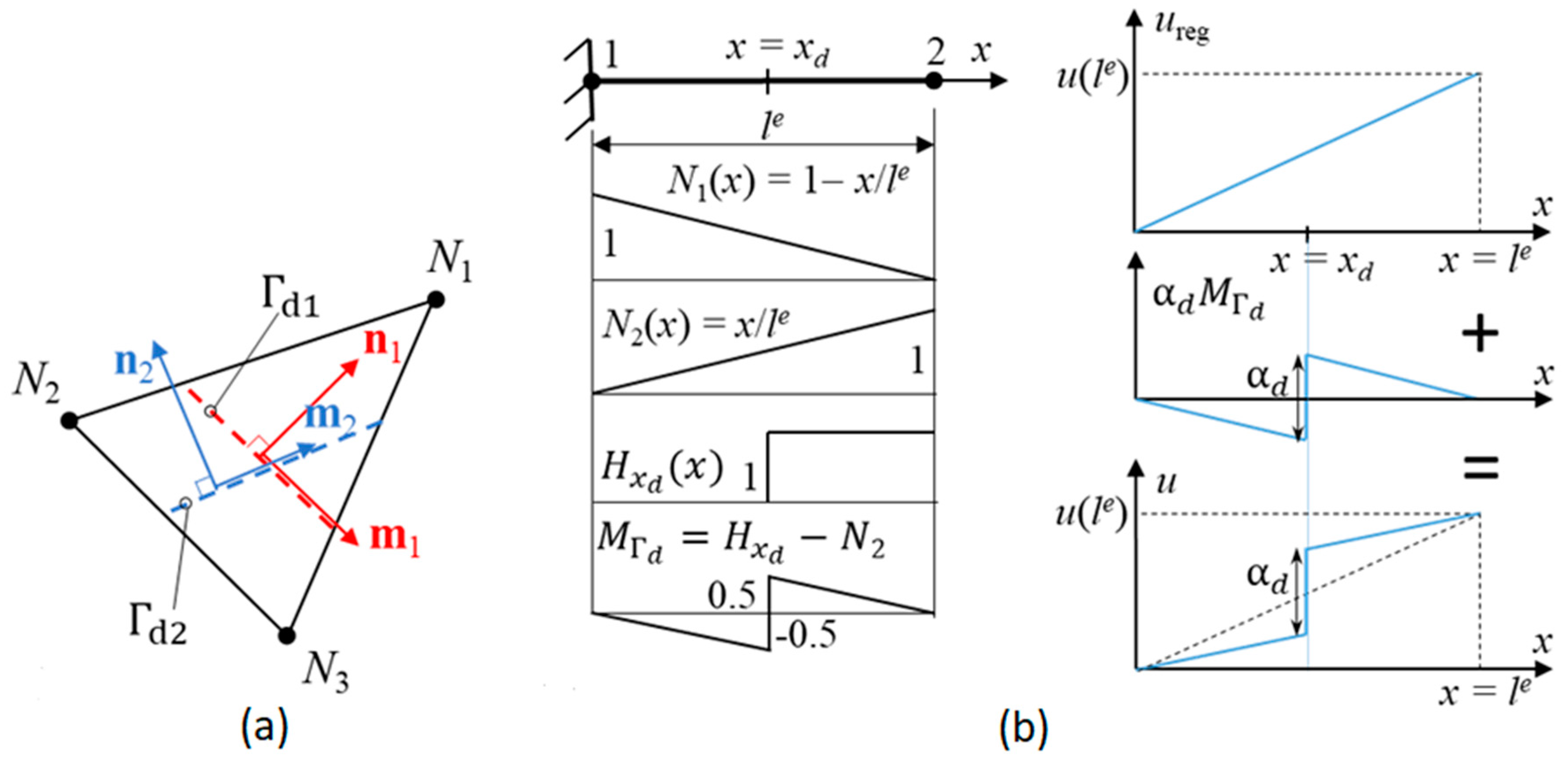
Considering a 2D body discretized with constant strain triangular (CST) finite elements having (possibly) intersecting cracks, i.e., displacement discontinuities, the discontinuities split some of the finite elements into two or more parts, as illustrated in Figure 1a. Two intersecting discontinuities are needed in the present application of modeling the effect of thermally induced cracks on the tensile strength of a rock specimen. More precisely, heat treatment of the numerical rock induces a substantial number of cracks with somewhat random orientations. As the fixed crack concept is adopted here (cracks do not rotate), an element with a crack unfavorably (close to parallel) oriented to the consequent uniaxial tension direction would generate spurious stresses without introducing the second crack.

Under the small strain assumption, the displacement and strain fields for such an element can be written as:

$$\mathit{u}\left(x\right)=N_i\left(x\right){\mathit{u}}_i^e+{\sum }_{i=1}^2{M}_{{\mathsf{\Gamma }}_{\mathrm{d}i}}\left(x\right){\mathsf{\alpha }}_{\mathrm{d}i} \mathrm{with} M_{{\mathsf{\Gamma }}_{\mathrm{d}i}}\left(x\right)=H_{{\mathsf{\Gamma }}_{\mathrm{d}i}}\left(x\right)-{\phi }_{{\mathsf{\Gamma }}_{\mathrm{d}i}}\left(x\right), \left(i=1,2\right)$$

(1)

$$\mathsf{\epsilon }\left(x\right)={\left(\nabla N_i\otimes {\mathit{u}}_i^e\right)}^{sym}-{\sum }_{i=1}^2\left({\left(\nabla {\phi }_{{\mathsf{\Gamma }}_{\mathrm{d}i}}\left(x\right)\otimes {\mathsf{\alpha }}_{\mathrm{d}i}\right)}^{sym}+{\delta }_{{\mathsf{\Gamma }}_{\mathrm{d}i}}{\left(n_i\otimes {\mathsf{\alpha }}_{\mathrm{d}i}\right)}^{sym}\right),$$

(2)

where ${\mathsf{\alpha }}_{\mathrm{d}i}$ is the displacement jump (crack opening) for crack i, and $N_i$ and ${\mathit{u}}_i^e$ are the standard interpolation functions for the CST element and nodal displacements (i = 1,…, 3 with summation on repeated indices), respectively. Moreover, $H_{{\mathsf{\Gamma }}_{\mathrm{d}i}}$ and ${\delta }_{{\mathsf{\Gamma }}_{\mathrm{d}i}}$ denote, respectively, the Heaviside function and its gradient, the Dirac delta function. Consistent with the constant strain of the linear triangle element, the displacement jump is likewise an assumed elementwise constant, which means that $\nabla {\mathsf{\alpha }}_{\mathrm{d}i}\equiv 0$, and thus (2) follows in a straightforward manner by taking the gradient of (1). Moreover, the terms containing the Dirac’s delta function, ${\delta }_{{\mathsf{\Gamma }}_{\mathrm{d}i}}{\left(n_i\otimes {\mathsf{\alpha }}_{\mathrm{d}i}\right)}^{sym}$, in (2), are non-zero only when $x \in {\mathsf{\Gamma }}_{\mathrm{d}i}$. Outside the discontinuity, this term is zero and can thus be neglected at the global level when solving the discretized equations of motion.

Function $M_{{\mathsf{\Gamma }}_{\mathrm{d}i}}$ in (1) restricts the effect of ${\mathsf{\alpha }}_{\mathrm{d}i}$ inside the corresponding finite element. This substantially facilitates the finite element implementation of the kinematics as there is no need for special treatment of the essential boundary conditions. The ramp function ${\phi }_{{\mathsf{\Gamma }}_{\mathrm{d}i}}$ appearing in $M_{{\mathsf{\Gamma }}_{\mathrm{d}i}}$ is chosen, from among the combinations of the nodal interpolation functions so that its gradient is as parallel as possible to the crack normal $n_i$:

$$\nabla {\phi }_{{\mathsf{\Gamma }}_{\mathrm{d}i}}=\arg \left(\underset{k=1,2}{\max }\frac{\left|{\sum }_{n=1}^k\nabla N_n·n_i\right|}{\Vert {\sum }_{i=1}^k\nabla N_n\Vert }\right), \left(i=1,2\right)$$

(3)

The displacement decomposition (1) and the related functions in the 1D case are illustrated in Figure 1b with a single two-node bar element under tension. On the left, the functions involved in the decomposition are plotted. The decomposition consists of the regular nodal displacement, $u_{reg}=N_1{u}_1+N_2{u}_2$, and the enhanced, discontinuous part, ${\mathsf{\alpha }}_{\mathrm{d}}$, the effect of which is restricted inside the element by function $M_{{\mathsf{\Gamma }}_{\mathrm{d}}}$. In the 1D case, the selection of function φ is readily identifiable as the interpolation function of node 2, i.e., N₂.

The finite element formulation of the embedded discontinuity kinematics is based on the enhanced assumed strain concept (EAS). The details of the implementation are presented in [23,24]. Here, the resulting equations for the thermo-mechanical problem are presented as:

$${{\displaystyle \int }}_{{\mathsf{\Omega }}_e}\rho N_i{N}_j{\ddot{\mathit{u}}}_j\mathrm{d}\mathsf{\Omega }+{{\displaystyle \int }}_{{\mathsf{\Omega }}_e}\sigma \cdot \nabla N_i\mathrm{d}\mathsf{\Omega }=\mathbf{0},\hspace{1em}i,j=1,\dots ,N_{nodes}$$

(4)

$${{\displaystyle \int }}_{{\mathsf{\Omega }}_e}{c\rho N}_i{N}_j{\dot{\theta }}_j\mathrm{d}\mathsf{\Omega }+{{\displaystyle \int }}_{{\mathsf{\Omega }}_e}\nabla N_{i}k\nabla N_j{\theta }_j\mathrm{d}\mathsf{\Omega }-{{\displaystyle \int }}_{{\mathsf{\Omega }}_e}{Q}_{int}{N}_j\mathrm{d}\mathsf{\Omega }=0,\hspace{1em}i,j=1,\dots ,N_{nodes}$$

(5)

$${\varphi }_{\mathrm{d}i}\left(t_{{\mathsf{\Gamma }}_{\mathrm{d}i}}\right)=0,t_{{\mathsf{\Gamma }}_{\mathrm{d}i}}=\sigma ·n_i, i=1,2 (\mathrm{for} \mathrm{elements} \mathrm{with} \mathrm{crack}(\mathrm{s}\left)\right)$$

(6)

$$\mathbf{\sigma }=E:\left(\widehat{\mathsf{\epsilon }}-{\sum }_{i=1}^2{\left(\nabla {\phi }_{{\mathsf{\Gamma }}_{\mathrm{d}i}}\otimes {\mathsf{\alpha }}_{\mathrm{d}i}\right)}^{sym}-{\mathsf{\epsilon }}_{\theta }\right),$$

(7)

where $\widehat{\mathsf{\epsilon }}={\left(\nabla N_i\otimes {\mathit{u}}_i^e\right)}^{sym}$ and ${\mathsf{\epsilon }}_{\theta }=\mathsf{\alpha }\Delta \theta I$ are the thermal strain, with α being the thermal expansion coefficient, $\Delta \theta$ the temperature change, and I the unit tensor. Moreover, ${\ddot{\mathit{u}}}_j$ is the acceleration vector, $N_{nodes}$ is the number of nodes in the mesh, and $N_i$ is the interpolation function of node i. In addition, $\sigma$ is the stress tensor, ${\dot{\theta }}_j$ is the rate of change of the temperature vector, ${\theta }_j$, at node j, $\rho$ and c are the density and the specific heat capacity of the material, k is the conductivity, and $Q_{int}$ is the internal heat production. Equation (4) is the discretized form of the balance of the linear momentum in the absence of external forces, while Equation (5) is the discretized equation of heat balance. The first equation in Equation (6), with ${\varphi }_{\mathrm{d}i}$ being the loading function to be defined in the next section, defines the elastic zone of stresses. Moreover, the second equation in (6) is the traction balance over the cracks with $t_{{\mathsf{\Gamma }}_{\mathrm{d}i}}$ being the traction for crack i. Finally, Equation (7) defines the constitutive relation for the material, with $E$ being the elasticity tensor. It is noted that Equations (4)–(7) have contributions from only the external heat influx, $Q_{int}$, which simulates heating in an oven. All other heat generation types, such as thermo-elastic (in the bulk material) and thermo-plastic heat generation (at the crack due to opening dissipation), are neglected as insignificant in comparison to the external heat influx [15]. It should be emphasized that this EAS-based formulation results in a simple implementation without the need to explicitly know the exact position of the discontinuity within the element or its length.

The present model describes the rock behavior as linear elastic upon reaching the tensile strength. When the first principal stress exceeds the tensile strength, a crack (displacement discontinuity) is introduced with a normal parallel to the first principal direction. As Equations (4), (6), and (7) are formally similar to the corresponding equations in plasticity theory, the problem of solving the irreversible crack opening increment and the evolution equations can be recast in the computational plasticity format [23]. The relevant model components, i.e., the loading function, softening rules, and evolution laws are defined as

$${\varphi }_{\mathrm{d}i}\left(t_{{\mathsf{\Gamma }}_{\mathrm{d}i}},{\kappa }_{\mathrm{d}i},{\dot{\kappa }}_{\mathrm{d}i}\right)=n_i·t_{{\mathsf{\Gamma }}_{\mathrm{d}i}}+\mathsf{\beta }\left|m_i·t_{{\mathsf{\Gamma }}_{\mathrm{d}i}}\right|-\left({\sigma }_{\mathrm{t}i}+q_{\mathrm{d}i}\left({\kappa }_{\mathrm{d}i},{\dot{\kappa }}_{\mathrm{d}i}\right)\right),$$

(8)

$$q_{\mathrm{d}i}=h_{\mathrm{d}i}{\kappa }_{\mathrm{d}i}+s_{\mathrm{d}}{\dot{\kappa }}_{\mathrm{d}i},h_{\mathrm{d}i}=-g_{\mathrm{d}}{\sigma }_{\mathrm{t}}\exp \left(-g_{\mathrm{d}}{\kappa }_{\mathrm{d}i}\right),g_{\mathrm{d}}=\frac{{\sigma }_{\mathrm{t}}}{G_{\mathrm{Ic}}},$$

(9)

$${\dot{t}}_{{\mathsf{\Gamma }}_{\mathrm{d}i}}=-E:\left(\nabla {\phi }_{{\mathsf{\Gamma }}_{\mathrm{d}i}}\otimes {\dot{\mathsf{\alpha }}}_{\mathrm{d}i}\right)·n_i,$$

(10)

$${\dot{\mathsf{\alpha }}}_{\mathrm{d}i}={\dot{\lambda }}_{\mathrm{d}i}\frac{\partial {\varphi }_{\mathrm{d}i}}{\partial {\mathbf{t}}_{{\mathsf{\Gamma }}_{\mathrm{d}i}}}, {\dot{\kappa }}_{\mathrm{d}i}=-{\dot{\lambda }}_{\mathrm{d}i}\frac{\partial {\varphi }_{\mathrm{d}i}}{\partial q_{\mathrm{d}i}},$$

(11)

$${\dot{\lambda }}_{\mathrm{d}i}\ge 0,{\varphi }_{\mathrm{d}i}\le 0,{\dot{\lambda }}_{\mathrm{d}i}{\varphi }_{\mathrm{d}i}=0, \left(i =1,2\right)$$

(12)

where ${\kappa }_{\mathrm{d}i}, {\dot{\kappa }}_{\mathrm{d}i}$ are the internal variable and its rate related to softening law $q_{\mathrm{d}i}$ for discontinuity i, and σ_ti is the tensile strength while s_d is the viscosity modulus. Parameter $h_{\mathrm{d}i}$ is the softening modulus of the exponential softening law, and parameter $g_{\mathrm{d}}$ controls the initial slope of the softening curve and it is calibrated by the mode I fracture energy, G_Ic. Moreover, ${\dot{\lambda }}_{\mathrm{d}i}$ is the crack opening increment. The loading function (8) has a shear term multiplied with shear parameter β. Finally, Equation (12) gives the Kuhn–Tucker conditions imposing the consistency. Therefore, these equations can be integrated using the standard algorithms of computational plasticity [15,23,24].

2.2. Solution of the Thermo-Mechanical Problem Governing the Thermal Treatment of Rock

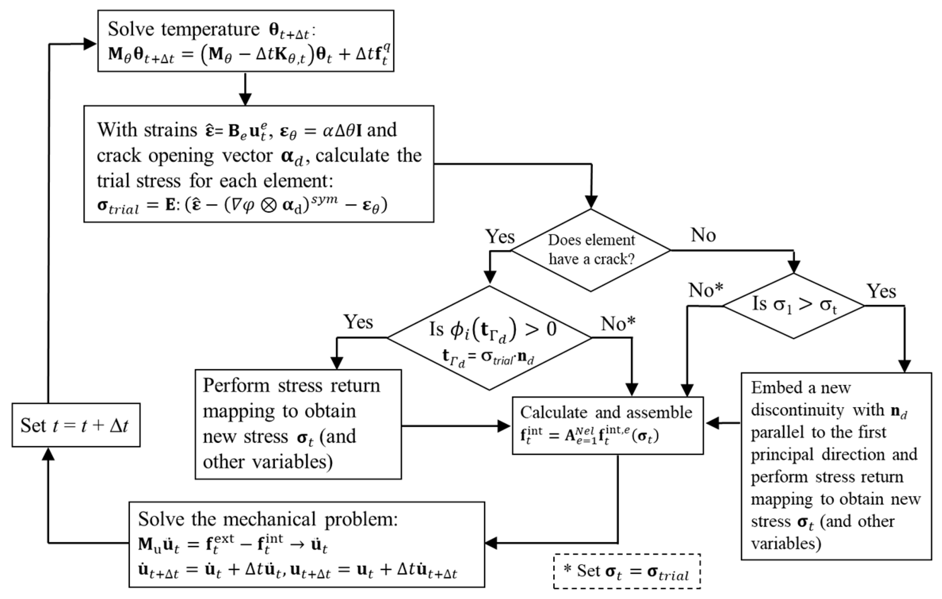
Equations (4) and (5) are solved with a staggered algorithm [25], first solving the temperature field while keeping the mechanical fields fixed, and then solving the mechanical fields while fixing the temperature field. Equations (6) and (7) are solved locally, in a manner similar to plasticity. The solution process with explicit time marching is illustrated in Figure 2.

The equation in Figure 2 for solving the temperature and the mechanical response are Equations (4) and (5) written in a matrix form. Moreover, the asterisk means that the trial prediction does not violate the loading function or that it does not exceed the tensile strength. As the critical time step of the explicit time marching of the mechanical problem is extremely small, many orders of magnitude smaller than that of the thermal problem, mass scaling is used here when solving the mechanical problem.

2.3. Solution of the Mechanical Problem Governing the Uniaxial Tension Test on Heated Rock

The mechanical uniaxial tension test on heated numerical rock is carried out by explicit time marching simulation using the same scheme as in Figure 2 for solving the mechanical problem. Moreover, a criterion for introducing a new crack in an element with an unfavorably oriented thermally induced crack is needed here. The criterion in [26] is used here with a modified tensile strength for the new crack. Accordingly, a new crack is introduced in an element already having a crack when the following criterion is fulfilled:

$$\mathrm{If} {\sigma }_1>{\sigma }_{\mathrm{t}}^{*} \& \left|n_1·n^{*}\right|<C_{\mathsf{\alpha }} \mathrm{with}$$

(13)

$${\sigma }_{\mathrm{t}}^{*}=\left(1-\left|n_1·n^{*}\right|\right){\sigma }_{\mathrm{t}}^{ic}+\left|n_1·n^{*}\right|{\sigma }_{\mathrm{t}0}$$

(14)

where $n_1$ is the normal of the initial crack, $n^{*}$ is the principal direction corresponding to the present major principal stress, ${\sigma }_1$. The modified tensile strength, ${\sigma }_{\mathrm{t}}^{*}$, is a convex combination of the strength of the initial crack, ${\sigma }_{\mathrm{t}}^{ic}$, and the intact tensile strength, ${\sigma }_{\mathrm{t}0}$. The meaning of the second inequality in (13) is that the new crack is introduced (only once) when the angle between the old crack normal and the new principal direction is greater than $\mathsf{\alpha }=\mathrm{acos}(C_{\mathsf{\alpha }})$, with $C_{\mathsf{\alpha }}$ being an adjustable parameter. A value of $1/\sqrt{2}$ corresponding to $\mathsf{\alpha }=45°$ is used in this study.

3. Numerical Simulations

The numerical simulations related to the thermal treatment of rock and its effect on the uniaxial tensile strength of rock are carried out here. First, however, the material properties and the model parameters are given. Moreover, the temperature dependency of the material properties is specified. All the simulations are carried out with a self-written MATLAB code.

3.1. Material Properties and Model Parameters

The homogenized mechanical and thermal properties for granite taken from [11] are: Young’s modulus E = 37.35 GPa; Poisson’s ratio ν = 0.127; density ρ = 2650 kg/m³; thermal expansion coeff. α₀ = 8E−6 K⁻¹; specific heat c = 820 J/kgK; and thermal conductivity k = 2.6 W/mK.

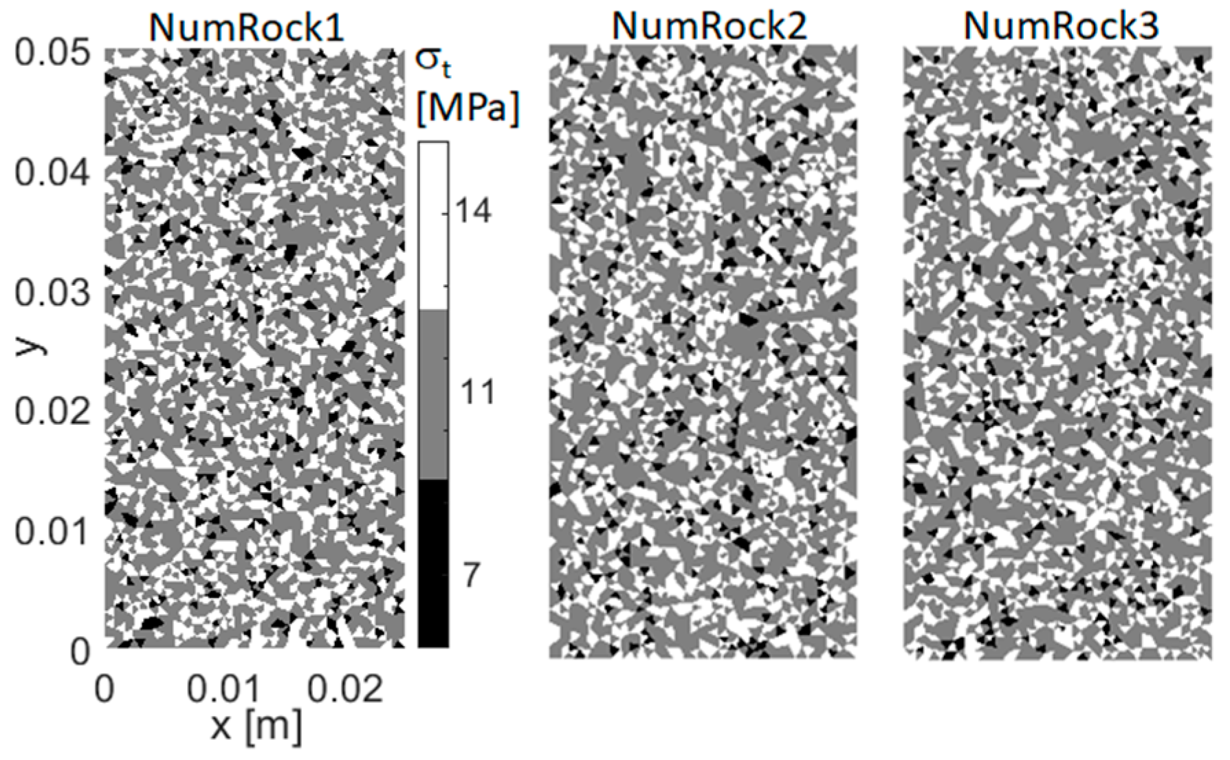
To properly predict the failure mode in tension, the tensile strength is assumed to be heterogeneous, i.e., mineral specific. In this respect, the numerical rock consists of quartz (33%), feldspar (59%) and biotite (8%) minerals, with their respective tensile strengths [27] of 14 MPa, 11 MPa and 7 MPa. Moreover, the mode I specific fracture energies, G_Ic, are [28] 40 J/m² for quartz and felspar, and 28 J/m² for biotite. The rock strength heterogeneity is described by random clusters of finite elements assigned with these strength properties. The numerical rock mesostructures (consisting of 4276 elements) thus generated to be used in the simulations are shown in Figure 3. Finally, the shear effect parameter is β = 1, and the viscosity is set to s_d = 0.001 MPa⋅s/m.

As mentioned in the Introduction, the temperature dependence of the material parameters is reduced to that of the thermal expansion. The tensile strength of granite at elevated temperatures is measured for a specimen and is first heated slowly to the target temperature and then cooled down to room temperature. This heat treatment induces cracks in the sample, leading to degradation of its tensile strength. For heterogeneous brittle materials with inherent flaws (e.g., microcracks), the tensile strength is an emerging property, representing the sample integrity under extensional loading, not a material property per se at the material point level. Therefore, it would beg the question to feed the experimental tensile strength at certain temperature into the material point level constitutive law and then predict that same strength.

Thereby, the mechanical and thermal properties, except for the thermal expansion coefficient, are assumed temperature independent during heat treatment simulations. The thermal expansion coefficient of quartz depends on temperature, as follows:

$${\mathsf{\alpha }}_q\left(\theta \right)={\mathsf{\alpha }}_{q0}\left(1+\frac{0.75}{823-293}\right)\left(\theta -293\right),\left[1/K\right]$$

(15)

where ${\mathsf{\alpha }}_{q0}$ is the thermal coefficient at room temperature. According to (15), the thermal expansion of quartz depends linearly on a temperature in the range of 20–550 °C. This is of course not fully realistic (see [7]) but a consequence of the present simplified modeling approach of using homogenous material properties (except the tensile strength) and reducing all the temperature dependent heterogeneity to that of quartz, as mentioned above. However, it will be shown that this approach predicts the thermal weakening effect with a reasonable accuracy.

3.2. Simulations of Rock Heat Treatment

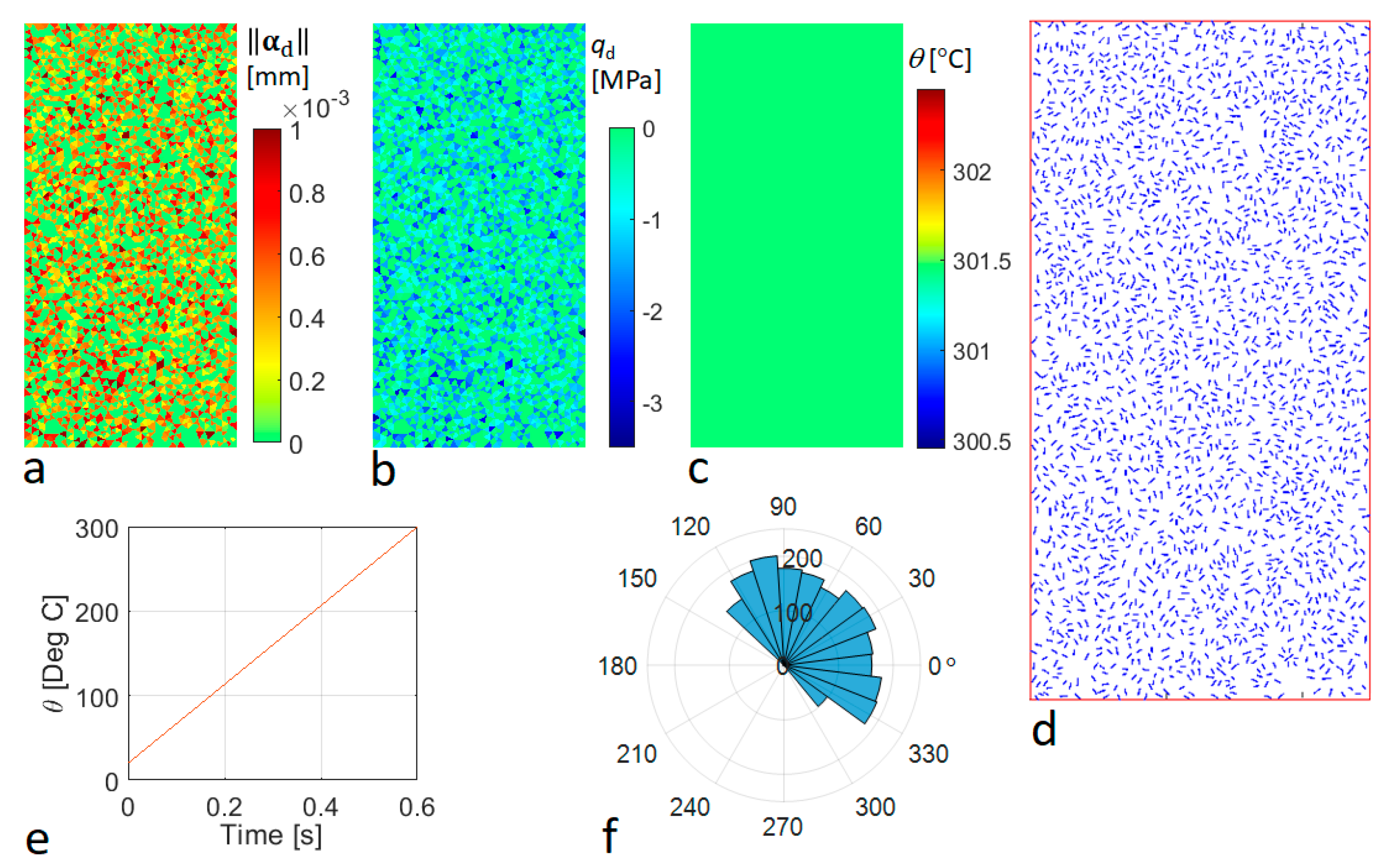
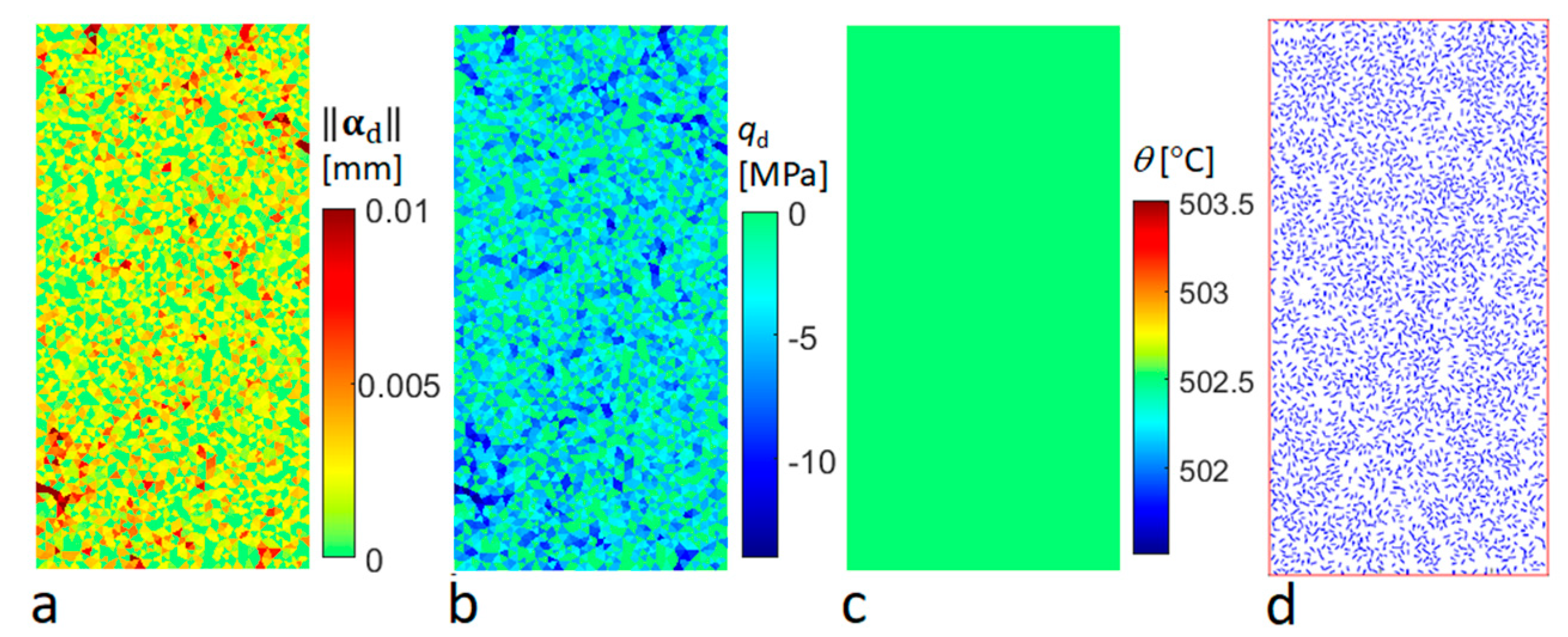
The numerical rock samples are heated uniformly to target temperatures of 300 °C and 500 °C. As the slow heating of rock does not induce inertia forces, extreme mass scaling can be used for the mechanical problem. Specifically, a million-fold density is used to increase the critical time step of the explicit time marching 1000-fold. In order to secure a uniform target temperature in the numerical sample, volume heating is applied here by specifying $Q_{int}$ = 1E9 W/m³ at each node of the finite element mesh. This value is chosen such that the target temperature of 500 °C is reached at every node of the mesh in 14,000 time steps. The duration of the simulation is, thus, 1 s. Simulation results for the numerical rock, NumRock1 in Figure 3, with the target temperature of 300 °C are shown in Figure 4.

The results in Figure 4c show that the final temperature distribution (≈301.5 °C) is uniform. The resulting number of cracks is 2186, i.e., about 50% of the elements have a crack at the end of heating. The orientation of the cracks (Figure 4c) is quite uniformly distributed between −40° and 140°. At this temperature, a crack opening (Figure 4a) is quite modest so the minimum value of the stress-like softening variable $q_{\mathrm{d}}$ is ~ −3.5 MPa, which means that the corresponding crack still has most of its load bearing capacity retained (see Equation (8)). The results were similar with those of numerical rocks 2 and 3 (Figure 3) so there is no need the plot the results. The simulation was then carried out further in time so that the target temperature 500 °C was reached. Some relevant results are shown in Figure 5 for numerical rock 1.

When heating is continued to 502.5 °C, the number of cracks increased from 2186 (in Figure 4) to 3098. As the difference between the thermal expansion coefficients of quartz and the other minerals increase with temperature, the crack opening magnitudes are much higher here (note the 10-fold range in Figure 5a compared to Figure 4a). This, in turn, leads to substantial softening, as can be observed in Figure 5b, where the minimum value of the stress-like softening variable reaches almost −14 MPa in some elements representing quartz.

3.3. Simulations of Uniaaxial Tension Test of Intact and Heat Treated Rock

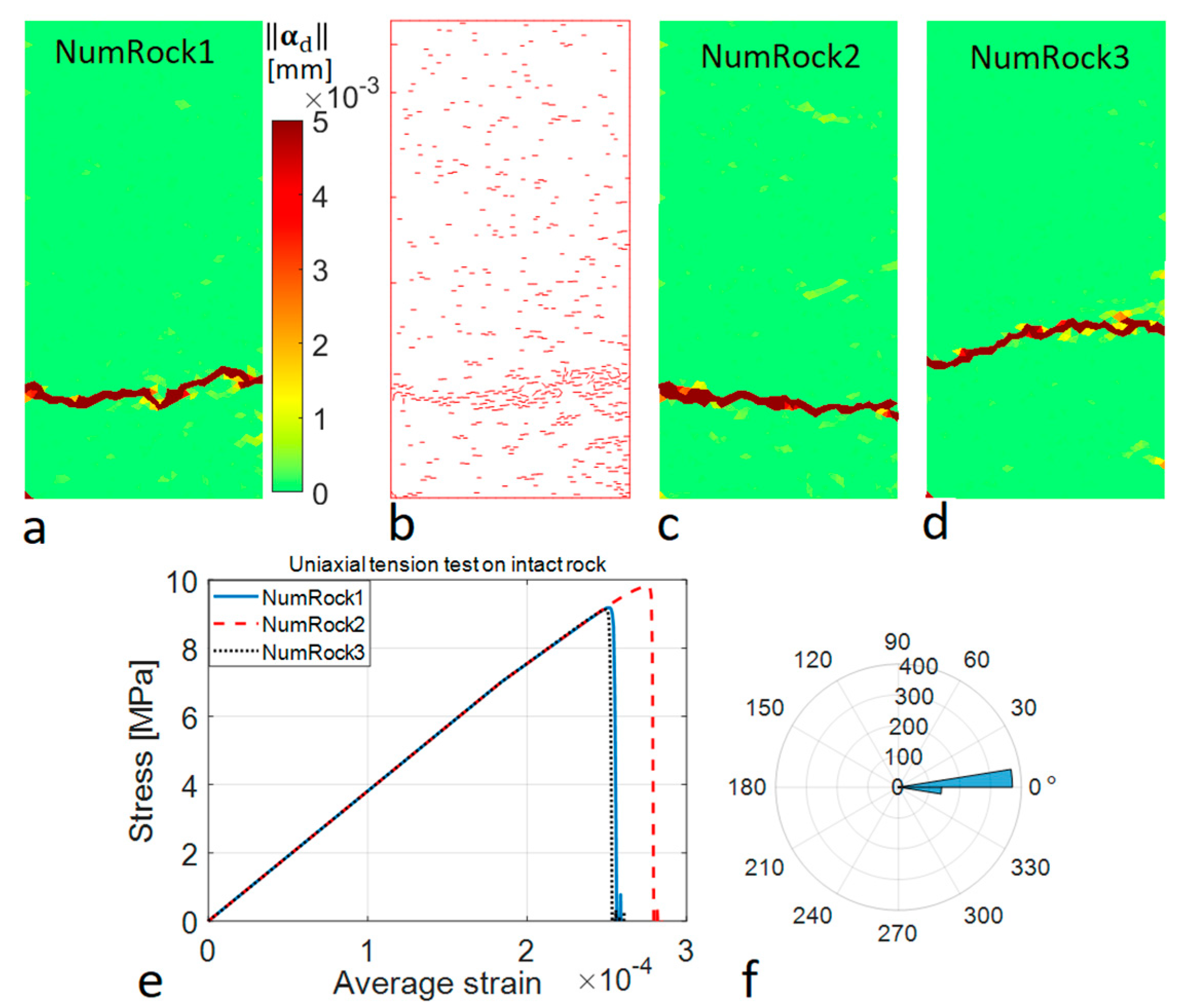
First, a uniaxial tension test is carried out on intact rock. The loading is applied as a constant velocity boundary condition at the upper edge of the specimen. The velocity is set to 5 mm/s, which means a strain rate of 0.1 s⁻¹ with the present sample size. The results for the numerical rocks in Figure 3 are shown in Figure 6.

All the numerical rock samples show the experimental transversal splitting failure mode with differing details. Cracks, 565 in total, appear all over the sample (Figure 6b). Only some of them open to form the final failure plane. Moreover, the crack orientation is mostly horizontal (Figure 6f). The predicted tensile strengths vary from 9.1 to 9.8 MPa. A slight pre-peak bent can be observed in the average stress–strain curves when the stress is 7 MPa. This corresponds to the failures (microcrack events) of biotite grains. After the peak stress, very brittle failure of the sample is attested in each case.

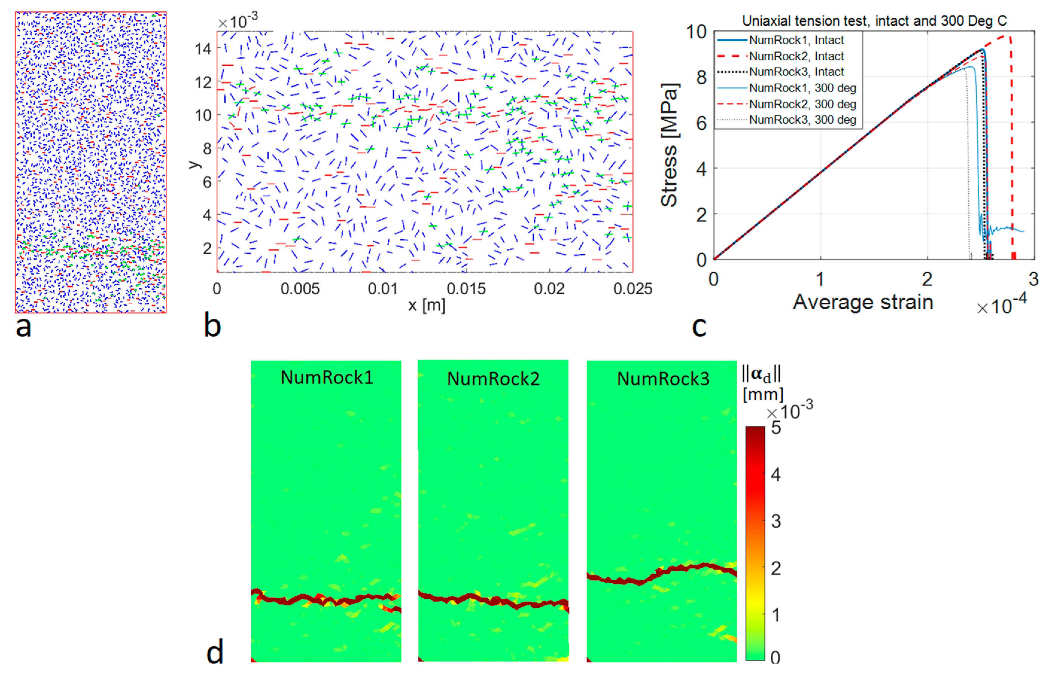
Next, a uniaxial tension test is carried out on the heat-treated samples. In order to mimic the experiments, these simulations are performed on the cooled down specimens. Thus, no thermal stresses exist in the sample. Moreover, it is assumed that the cracks are closed, meaning that their opening vectors are nullified but their orientations and residual strengths are included in the initial state here. Thereby, the residual tensile strength for an element with a crack is calculated by ${\sigma }_{\mathrm{t}0}+q_{\mathrm{d}}$ where ${\sigma }_{\mathrm{t}0}$ is the intact tensile strength of the mineral and $q_{\mathrm{d}}$ is the stress-like softening variable at the end of the heat treatment simulations. The simulation results for the target temperature of 300 °C is shown in Figure 7.

The weakening effect of the thermal cracks induced by heating to 300 °C is not very strong. Indeed, the tensile strength of the heated samples is about 90% that of the intact one (Figure 7c). Moreover, the failure modes differ only in details from the intact ones (compare Figure 7d to Figure 6. As to the cracks plotted for the numerical rock 1 in Figure 7a,b, many new cracks (green color) have initiated in elements already having an unfavorably oriented thermally induced crack (blue color). Between the thermal cracks, a considerable number of new horizontal cracks, due to the tensile loading, have initiated. Next, the simulations were re-performed continuing the heating up to 500 °C. The results are plotted in Figure 8.

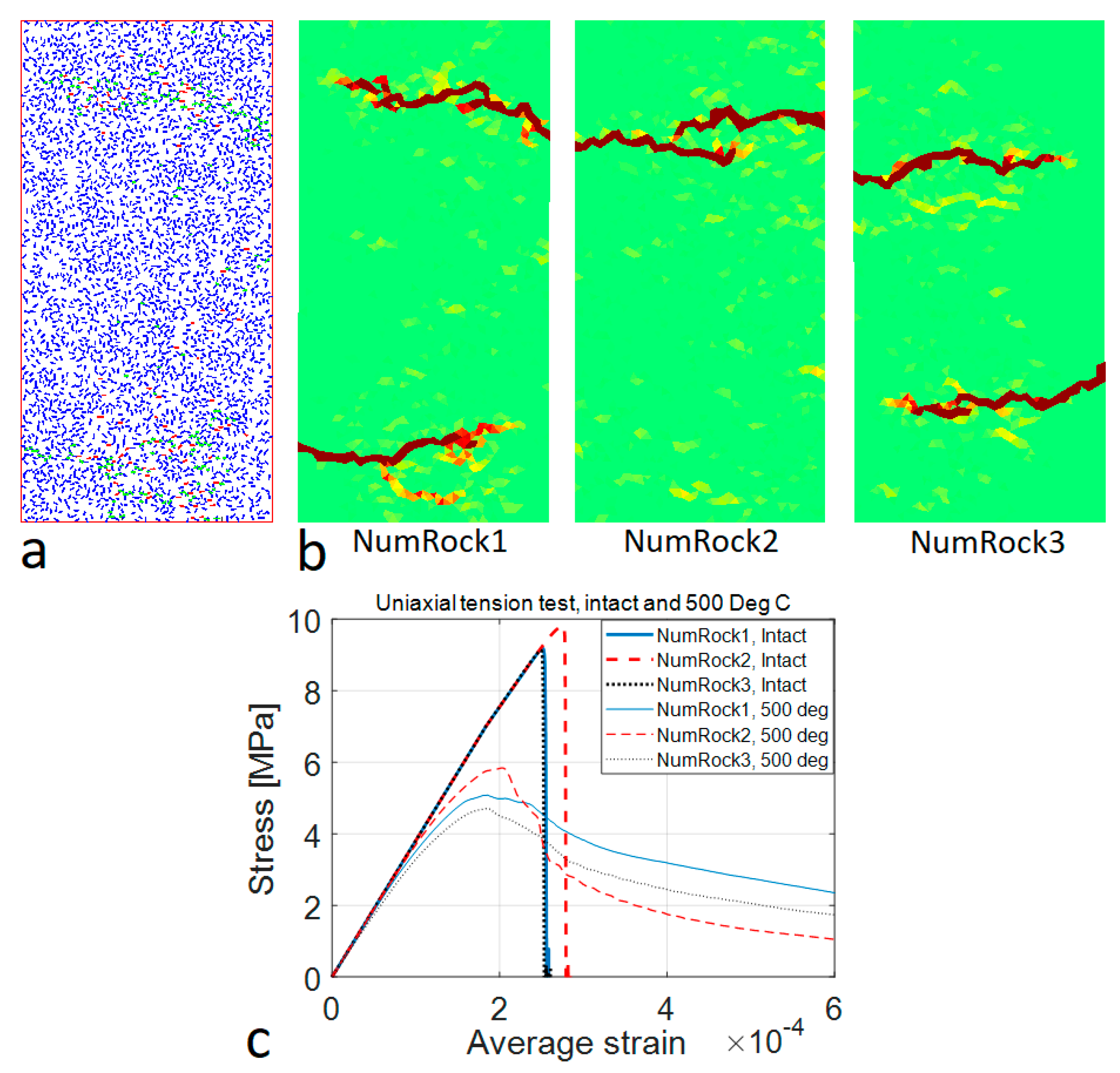
When the heating is continued to 500 °C, the weakening effect is substantial, as seen in the average stress–strain curves in Figure 8c. Moreover, the pre-peak nonlinear part of the curves is much more pronounced than those at 300 °C. This is due to the opening of the thermally induced cracks, which have reduced tensile strengths, during uniaxial tension loading. Furthermore, the post-peak softening part of the average responses is much more ductile due to dissipation occurring through the opening of a considerable number of cracks. The corresponding failure modes attest to the overlapping double-crack mode, where the major cracks initiate at the vertical edges of the sample and propagate inwards at different height levels, thus never coalescing, except for NumRock2 in the present case.

4. Discussion

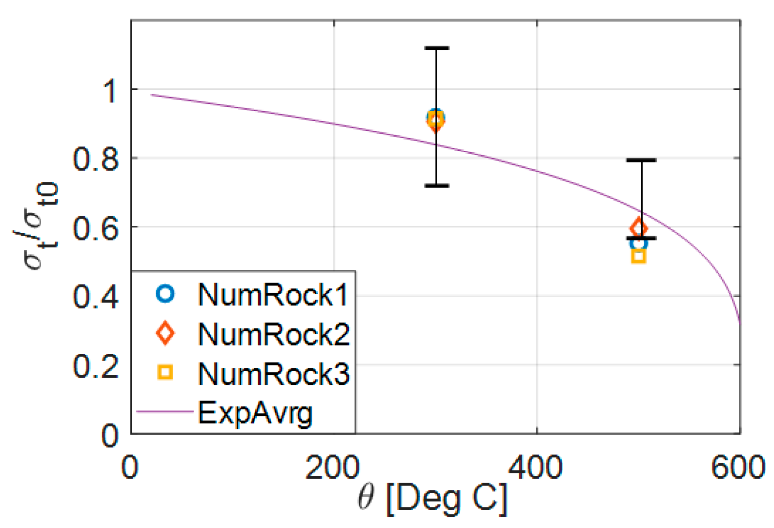
The aspects of the modeling approach and the results are discussed here. The simulation results are first compared to experimental observations. To this end, the predicted normalized tensile strengths are plotted as a function of temperature in Figure 9, along with the experimental data collected in [11].

The weakening effect predicted with the present approach is within the experimental deviation for several granites, except the a slight overprediction at 500 °C, which could be easily mended by fine tuning the thermal expansion coefficient (15). It should be noted that the curve, $f_{{\sigma }_{\mathrm{t}}/{\sigma }_{\mathrm{t}0}}=0.9912{\left(1-4.10\theta /2483.30\right)}^{1/4.10}$, in Figure 9 representing the average of the experimental results for several granites [11] is averaged over a wide range of test temperatures—hence it does not cross the deviation bars at the middle. Moreover, only relevant deviation bars, i.e., those at 300 °C and 500 °C, are shown in Figure 9.

Then some aspects of the numerical approach are discussed. The present approach falls within the class of continuum models, thus having all the advantages, over the discontinuum approach, of this class, such as the maturity of the method (FEM), the ease of calibration and the physical meaning of the model parameters, and, most importantly, the computational effectiveness. Moreover, the poor crack description of the continuum approach (FEM) is improved by the embedded discontinuity technology which is capable of representing cracking in rocks.

A staggered explicit approach was employed in simulating the slow heating of rock samples up to a uniform target temperature. As this process, which takes several hours in a lab, is quasi-static in nature, extreme mass scaling using a million-fold density for the mechanical part of the problem, resulting in a 1000-fold critical time step, could be used. This aspect combined with volume heating of the sample resulted in a simulation method capable of performing this kind of simulation in practical CPU times, even with fully explicit time marching. Moreover, the fully explicit method evades the convergence problems related to the Newton–Raphson iteration involved in the implicit methods, which, however, are unconditionally stable in time.

The thermal weakening effect of elevated uniform temperatures in rock samples is caused by heterogeneity, which becomes more pronounced in granites due to the deviant behavior of quartz. In the present approach, only the tensile strength heterogeneity of rock-forming minerals was included, while homogenized values for the elastic and thermal properties were used. All heterogeneity effects were reduced to accounting only for the temperature dependence of the quartz thermal expansion using a linear fit representing the net effect between quartz and the rest of the granite-forming minerals (feldspars and micas). This simplified approach has the advantage that it uses the easily measurable mechanical and thermal properties of a rock sample, instead of the far more effort needing properties of constituent minerals. Anyways, this approach appeared to work very well, as the weakening effect of thermal cracking on the tensile strength of granite was predicted with a surprisingly good accuracy. It should be emphasized that the weakening effect was predicted in a non-circular way, i.e., without using the experimental data on the temperature dependence of the tensile strength of granite as a model input.

However, the present approach ignores most of the textural aspects of rock as a polycrystalline material. In particular, the grain boundaries were not accounted for. Where their inclusion is deemed crucial, more detailed models, such as the DEM mentioned in the Introduction, should be applied. Another possibility within the continuum approach is to use the cohesive elements between the groups of finite elements representing the grains. However, this would require substantially more detailed data on the rock mineral texture and the mechanical properties thereof.

5. Conclusions

A numerical method to predict thermal cracking induced weakening effects in the tensile strength of granitic rock was developed and validated in this paper. The following conclusions can be drawn:

• The nonlinear coupled problem of thermal cracking in rock due to a uniform elevated temperature field can be effectively solved with an explicitly staggered approach. The present method, based on embedded discontinuity finite elements, is computationally fast and has physically meaningful model parameters.
• Extreme mass scaling for the mechanical problem can be used in this approach due to the quasi-static nature of the slow heating of a rock sample to a uniform temperature. Particularly, a million-fold density, to increase the critical time step 1000-fold, can be used with virtually no effect on accuracy.
• In modeling, thermal cracking induced reduction of tensile strength of granitic rocks due to a uniform temperature field can be reduced to the deviant behavior of the quartz mineral. This means that it is enough to account for only the temperature dependence of the quartz thermal expansion. Moreover, homogenous and temperature-independent mechanical properties, measured for a rock sample, can thus be used. However, the initial (room temperature) tensile strength parameters should be heterogenous to correctly predict the failure mode in uniaxial tension.
• With this method, the thermal weakening effect can be replicated in a non-circular way, i.e., without using the experimental data on the temperature dependence of the tensile strength of granite as a model input.
• The purpose of the present modelling approach is a fast prediction of the tensile strength degradation of a granite rock under elevated uniform temperature with a small set of easily measurable parameters of the target rock.

In closing, some further research topics concerning the present approach are suggested. First, this study addressed only the thermal weakening of tensile strength. However, natural rocks are most often under compression. Therefore, the thermal weakening of compressive strength should also be addressed in further studies. However, this requires a compressive failure criterion and is thus not a trivial task. Second, the heterogeneity of rock mineral elasticity, which was neglected, has effects that cannot be ignored at the mesoscale of interest. For this reason, this aspect should be included into the model in further considerations. Third, an explicit staggered method was employed in solving the governing thermo-mechanical equations. Notwithstanding, an implicit method would have the advantages of being unconditionally stable in time and would provide more reliable results. Therefore, an implicit version should be developed in future. Finally, the present study was carried out under simplified 2D assumptions. A 3D version of the present study should thus be performed to confirm the results.

References

- Kumari, W.G.P.; Ranjith, P.G.; Perera, M.S.A.; Shao, S.; Chen, B.K.; Lashin, A.; Arifi, N.A.; Rathnaweera, T.D. Mechanical behaviour of Australian Strathbogie granite under in-situ stress and temperature conditions: An application to geothermal energy extraction. Geothermics 2017, 65, 44–59. [Google Scholar] [CrossRef]
- Heuze, F.E. Geotechnical Modeling of High-Level Nuclear Waste Disposal by Rock Melting (No. UCRL-53183); Lawrence Livermore National Lab.: San Francisco, CA, USA, 1981. [Google Scholar]
- Kant, M.A.; Rossi, E.; Madonna, C.; Höser, D.; von Rohr, P.R. A theory on thermal spalling of rocks with a focus on thermal spallation drilling. J. Geophys. Res. Solid Earth. 2017, 122, 1805–1815. [Google Scholar] [CrossRef]
- Carpenter, M.A.; Salje, E.K.H.; Graeme-Barber, A.; Wruck, B.; Dove, M.T.; Knight, K.S. Calibration of excess thermodynamic properties and elastic constant variations associated with the α-β phase transition in quartz. Am. Miner. 1998, 83, 2–22. [Google Scholar] [CrossRef] [Green Version]
- Gautam, P.K.; Verma, A.K.; Jha, M.K.; Sharma, P.; Singh, T.N. Effect of high temperature on physical and mechanical properties of Jalore granite. J. Appl. Geophys. 2018, 159, 460–474. [Google Scholar] [CrossRef]
- Heuze, F. High temperature mechanical, physical and thermal properties of granitic rocks—A review. Int. J. Rock Mech. Min. Sci. Geomech. Abstr. 1983, 20, 3–10. [Google Scholar] [CrossRef]
- Toifl, M.; Hartlieb, P.; Meisels, R.; Antretter, T.; Kuchar, F. Numerical study of the influence of irradiation parameters on the microwave-induced stresses in granite. Min. Eng. 2017, 103–104, 78–92. [Google Scholar] [CrossRef]
- Yang, S.Q.; Ranjith, P.G.; Jing, H.W.; Tian, W.L.; Ju, Y. An experimental investigation on thermal damage and failure mechanical behavior of granite after exposure to different high temperature treatments. Geothermics 2017, 65, 180–197. [Google Scholar] [CrossRef]
- Yin, T.; Shu, R.; Li, X.; Wang, P.; Liu, X. Comparison of mechanical properties in high temperature and thermal treatment granite. Trans. Nonferrous Met. Soc. China. 2016, 26, 1926–1937. [Google Scholar] [CrossRef]
- Vázquez, P.; Shushakova, V.; Gómez-Heras, M. Influence of mineralogy on granite decay induced by temperature increase: Experimental observations and stress simulation. Eng. Geol. 2015, 189, 58–67. [Google Scholar] [CrossRef]
- Wang, F.; Konietzky, H. Thermo-Mechanical Properties of Granite at Elevated Temperatures. and Numerical Simulation of Thermal Cracking. Rock Mech. Rock Eng. 2019, 52, 3737–3755. [Google Scholar] [CrossRef]
- Wang, F.; Konietzky, H.; Frühwirt, T.; Li, L.; Dai, Y. The Influence of Temperature and High-Speed Heating on Tensile Strength of Granite and the Application of Digital Image Correlation on Tensile Failure Processes. Rock Mech. Rock Eng. 2020, 53, 1935–1952. [Google Scholar] [CrossRef]
- Griffiths, L.; Heap, M.J.; Baud, P.; Schmittbuhl, J. Quantification of microcrack characteristics and implications for stiffness and strength of granite. Int. J. Rock. Mech. Min. Sci. 2017, 100, 138–150. [Google Scholar] [CrossRef]
- Zhao, Z.; Xu, H.; Wang, J.; Zhao, X.; Cai, M.; Yang, Q. Auxetic behavior of Beishan granite after thermal treatment: A microcracking perspective. Eng. Fract. Mech. 2020, 231, 107017. [Google Scholar] [CrossRef]
- Pressacco, M.; Saksala, T. Numerical modelling of thermal shock assisted rock fracture. Int. J. Numer. Anal. Methods. Geomech. 2020, 44, 40–68. [Google Scholar] [CrossRef]
- Raude, S.; Laigle, F.; Giot, R.; Fernandes, R. A unified thermoplastic/viscoplastic constitutive model for geomaterials. Acta Geotech. 2016, 11, 849–869. [Google Scholar] [CrossRef]
- Saksala, T. Numerical modelling of adiabatic heat generation during rock fracture under dynamic loading. Numer. Anal. Methods Geomech. 2019, 43, 1770–1783. [Google Scholar] [CrossRef]
- Jing, L.; Hudson, J.A. Numerical methods in rock mechanics. Int. J. Rock Mech. Min. Sci. 2002, 39, 409–427. [Google Scholar] [CrossRef]
- Nikolić, M.; Roje-Bonacci, T.; Ibrahimbegović, A. Overview of the numerical methods for the modelling of rock mechanics problems. Teh. Vjesn. 2016, 23, 627–637. [Google Scholar]
- Hamdi, P.; Stead, D.; Elmo, D. Characterizing the influence of stress-induced microcracks on the laboratory strength and fracture development in brittle rocks using a finite-discrete element method-micro discrete fracture network FDEM-μDFN approach. J. Rock. Mech. Geotech. 2015, 7, 609–625. [Google Scholar] [CrossRef] [Green Version]
- Simo, J.C.; Oliver, J.; Armero, F. An analysis of strong discontinuities induced by strain-softening in rate-independent inelastic solids. Comput. Mech. 1993, 12, 277–296. [Google Scholar] [CrossRef]
- Belytschko, T.; Black, T. Elastic crack growth in finite elements with minimal remeshing. Int. J. Numer. Meth. Eng. 1999, 45, 601–620. [Google Scholar] [CrossRef]
- Mosler, J. On advanced solution strategies to overcome locking effects in strong discontinuity approaches. Int. J. Numer. Meth. Eng. 2005, 63, 1313–1341. [Google Scholar] [CrossRef]
- Saksala, T.; Brancherie, D.; Harari, I.; Ibrahimbegovic, A. Combined continuum damage-embedded discontinuity model for explicit dynamic fracture analyses of quasi-brittle materials. Int. J. Numer. Meth. Eng. 2015, 101, 230–250. [Google Scholar] [CrossRef]
- Ottosen, N.S.; Ristinmaa, M. The Mechanics of Constitutive Modeling; Elsevier: Amsterdam, The Netherlands, 2005. [Google Scholar]
- Saksala, T.; Ibrahimbegovic, A. Thermal shock weakening of granite rock under dynamic loading: 3D numerical modelling based on embedded discontinuity finite elements. Int. J. Numer. Anal. Met. Geomech. 2020, 44, 1788–1811. [Google Scholar] [CrossRef]
- Zhao, D.; Zhang, S.; Wang, M. Microcrack Growth Properties of Granite under Ultrasonic High-Frequency Excitation. Adv. Civil Eng. 2019, 2019, 3069029. [Google Scholar] [CrossRef]
- Mahabadi, O.K. Investigating the Influence of Micro-Scale Heterogeneity and Microstructure on the Failure and Mechanical Behaviour of Geomaterials. Ph.D. Thesis, University of Toronto, Toronto, ON, Canada, August 2012. [Google Scholar]
Figure 1.
(a) CST element with two intersecting discontinuities (, : normal and tangent for crack 1, ; , : normal and tangent for crack 2, ; Ni: interpolation function at node i); (b) illustration of the displacement decomposition to regular and enhanced part and the corresponding functions in a 1D case ( : regular displacement; u: total displacement; ; displacement jump; : special function restricting the effect of inside the element).
Figure 2.
The flowchart of the global solution of the thermo-mechanical problem.
Figure 3.
Tensile strength distribution in numerical rock samples (quartz = white, feldspar = gray, biotite = black).
Figure 4.
Simulation results for heat treatment (300 °C, NumRock1): (a) crack opening magnitude; (b) stress-like softening variable; (c) temperature field; (d) thermally induced cracks; (e) temperature evolution in time; (f) polar histogram showing crack orientation angles (2186 cracks).
Figure 5.
Simulation results for heat treatment (500 °C, NumRock1): (a) crack opening magnitude; (b) stress-like softening variable; (c) temperature field; (d) thermally induced cracks (3098 cracks).
Figure 6.
Simulation results for uniaxial tension test (intact rock): (a) crack opening magnitude with NumRock1; (b) cracks with NumRock1; (c) crack opening magnitude with NumRock2; (d) crack opening magnitude with NumRock3; (e) average stress–strain curves; (f) polar histogram showing crack orientation angles (565 cracks) with NumRock1.
Figure 7.
Simulation results for uniaxial tension test (heat treated rock, 300 °C): (a) cracks with NumRock1; (b) close up detail (blue = thermal cracks, red = tensile cracks, green = new cracks in elements with a thermal crack); (c) average stress–strain curves; (d) failure models represented by crack opening magnitudes.
Figure 8.
Simulation results for uniaxial tension test (heat treated rock, 500 °C): (a) cracks with NumRock1; (b) failure modes represented by crack opening magnitude; (c) average stress–strain curves.
Figure 9.
Normalized tensile strength vs. temperature predictions (experimental averaged curve and the variation at 300 °C and 500 °C for different granites are reproduced after the data in [11]).
Publisher’s Note: MDPI stays neutral with regard to jurisdictional claims in published maps and institutional affiliations. |
© 2021 by the author. Licensee MDPI, Basel, Switzerland. This article is an open access article distributed under the terms and conditions of the Creative Commons Attribution (CC BY) license (https://creativecommons.org/licenses/by/4.0/).
Share and Cite
MDPI and ACS Style
Saksala, T. Numerical Modeling of Temperature Effect on Tensile Strength of Granitic Rock. Appl. Sci. 2021, 11, 4407. https://0-doi-org.brum.beds.ac.uk/10.3390/app11104407
AMA Style
Saksala T. Numerical Modeling of Temperature Effect on Tensile Strength of Granitic Rock. Applied Sciences. 2021; 11(10):4407. https://0-doi-org.brum.beds.ac.uk/10.3390/app11104407
Chicago/Turabian StyleSaksala, Timo. 2021. "Numerical Modeling of Temperature Effect on Tensile Strength of Granitic Rock" Applied Sciences 11, no. 10: 4407. https://0-doi-org.brum.beds.ac.uk/10.3390/app11104407
Note that from the first issue of 2016, this journal uses article numbers instead of page numbers. See further details here.