
Aggregate and Particle Size Distribution of the Soil Sediment Eroded on Steep Artificial Slopes


Department of Landscape Water Conservation, Faculty of Civil Engineering, Czech Technical University in Prague, 160 00 Prague, Czech Republic
*
Author to whom correspondence should be addressed.
Appl. Sci. 2021, 11(10), 4427; https://0-doi-org.brum.beds.ac.uk/10.3390/app11104427
Submission received: 13 April 2021
/
Revised: 4 May 2021
/
Accepted: 8 May 2021
/
Published: 13 May 2021
(This article belongs to the Special Issue Challenges and Solutions in Soil and Water Conservation)
Abstract
:In this study, the particle size distribution (PSD) of the soil sediment from topsoil obtained from soil erosion experiments under different conditions was measured. Rainfall simulators were used for rain generation on the soil erosion plots with slopes 22°, 30°, 34° and length 4.25 m. The influence of the external factors (slope and initial state) on the particle and aggregate size distribution were evaluated by laser diffractometer (LD). The aggregate representation percentage in the eroded sediment was also investigated. It has been found that when the erosion processes are intensive (steep slope or long duration of the raining), the eroded sediment contains coarser particles and lower amounts of aggregates. Three methods for the soil particle analyses were tested: (i) conventional–sieving and hydrometer method; (ii) PARIO Soil Particle Analyzer combined with sieving; and (iii) laser diffraction (LD) using Mastersizer 3000. These methods were evaluated in terms of reproducibility of the results, time demands, and usability. It was verified that the LD has significant advantages compared to other two methods, especially the short measurement time for one sample (only 15 min per sample for LD) and the possibility to destroy soil aggregates using ultrasound which is much easier than using hexametaphosphate.
1. Introduction
Soil erosion by water is commonly mentioned as a worldwide environmental problem. During a rainfall, the soil surface is disturbed by rain drops and surface runoff, the soil particles get mobilized and washed out of the surface [1]. The particle and aggregate size distribution of the eroded soil sediment could give us information about the erosion process and formation of the rills [2].
Topsoil is a non-renewable resource and a valuable asset of every country. Water erosion has very negative effect on the productivity of agricultural land and also on the service life of soil structure. It removes the most fertile topsoil, reduces the thickness of the soil profile and decreases the content of nutrients and soil organic matter. It causes significant degradation of agricultural soils and reduces the quality of surface water in which the eroded sediment is transported [3,4,5,6,7,8,9,10,11,12]. Therefore, the soil must be protected as much as possible from degradation and the negative effects of water erosion must be reduced. The processes of water erosion must be thoroughly researched and understood in order to protect soil and reduce soil erosion effectively.
The particle size distribution of the soil is given by the representation of individual mineral particles of different sizes. The soil is divided into fine soil and skeleton. Fine soil is formed by particles smaller than 2000 μm and affects the basic soil properties [12]. There are many classification systems for classifying soils according to their particle size. In the Czech Republic, Novak’s classification system is used which divides soils into seven soil categories, from sandy soils to the finest soils marked as clay, according to the representation of fine particles smaller than 10 μm [13]. The classification system USDA NRCS classifies soils using a triangular diagram for which the representation of the three basic fractions must be known: sand (50 μm–2000 μm), silt (2 μm–50 μm), and clay (smaller than 2 μm) [14]. Furthermore, ASTM Unified Soil Classification System (USCS) can be applied. The combination of two letters to classify the soil is used, the first letter represents PSD (gravel, sand, silt, clay, organic) and the second letter represents the texture (poorly graded, well-graded, high plasticity, low plasticity) [15].
The soil aggregates are formed by cementing soil particles with organic matter and other cementing agents, thus increasing the stability of the soil structure, which makes the soil more resistant to the erosion. The aggregate’s formation is influenced by many factors, like swelling pressure, capillary action, and biological and chemical cementing agents [16]. The organic matter increases the soil’s ability to retain water [17]. Pores formed between the aggregates may contain air or may be filled with a loose material and allow water to infiltrate through the soil. The infiltration of water through the soil aggregates is influenced by their spatial arrangement. The destruction of soil aggregates by rainfall leads to soil degradation and increased soil erosion [18]. The aggregate size distribution can be determined by using a laser diffractometer [19,20].
Recently, the popularity of laser diffraction for analyzing particle size distribution has increased. This method is faster than sedimentation methods, thus it is possible to analyze greater number of samples within the same time [21,22]. In previous studies comparing particle size analysis methods based on different physical principles, it was found that the usability of the methods to obtain particle size distribution differ in the type of soil that is measured, mainly in the particle shape characteristics [23,24,25,26,27,28]. The studies where the sedimentation methods and laser diffraction were compared conclude that the volume representation of the clay fraction obtained by laser diffraction was generally lower than the mass representation of the clay fraction derived by the pipette or hydrometer method, while an opposite trend was determined for the silt fraction [21,23,27,28,29,30,31]. Conclusions from the study of comparison of laser diffractometer and sieving method are that the sieving method underestimates particles which contain non-equant grain types compared to the laser diffraction, because grains with a width to length ratio of 0.5 can pass through smaller mesh size of the sieve [31]. Durner et al. [32] who presented an integral suspension pressure (ISP) method—this method is based on the temporal change of the pressure measured with high accuracy at a certain depth within the suspension to derive the particle size distribution—concluded that the results from the pipette method and the ISP method are in a very good agreement.
In previous studies, the impact of slope to the erosion processes was investigated. Shanshan et al. [33] found that if the slope is lower than 18°, the intensity of erosion processes increases equally to the degree of the slope. For slopes from 18° to 25° the relationship between the erosion and the degree of the slope is exponential. On the other hand, the erosion processes decrease for slopes higher than 25°. The higher the slope, the greater the influence of the rainfall intensity. The slopes of the experimental plots investigated by Jing et al. [34] were 35°, 40°, and 45°, and rainfall intensity was 102 mm/h. They concluded that with higher slope less water percolate to the soil which causes greater runoff and erosion effect.
Erosion processes are influenced by the aggregate stability (AGS) and possibilities of their disintegration [35]. Kasmerchak et al. [36] conclude the possibilities of the laser diffraction method in the studies of AGS. In most of the soil erosion studies, and in general, the size-selection of the sediment is recognized as a common natural process [37,38,39]. In another study, it was found that the fine particles were washed out during sheet flow and splash erosion, while the coarser particles were eroded during rill and interrill erosion [40].
The goal of this contribution was to achieve more detailed monitoring of the percentage representation of eroded aggregates and their distribution in individual soil fractions in relation to the slope gradient, precipitation duration, and the initial state. The research was focused on the bare soil on the steep slopes that are situated along linear engineering structures (road, railways, embankments). Many of recent studies have mainly been focused on soil erosion on cropland [33] where the slope is usually small. This study aims to investigate soil erosion processes on steep slope land, which has not been studied thoroughly before. Also, our study benefits from the large sizes of the experimental plots, which ensures good reliability of the results.
In this study, three different methods to determine particle size distribution were compared to find the best suitable method for this research.
2. Materials and Methods
In this contribution, the particle size distribution of the soil sediment eroded from experimental plots during rainfall experiments was analyzed and three different methods to determine particle size distribution were compared, i.e., hydrometer (GECO, Bochum, Germany), PARIO Soil Particle Analyzer (METER Group, München, Germany) and laser diffractometer Mastersizer 3000 (Malvern Instruments, Malvern, UK).
2.1. Experimental Setup
The data for this research were obtained from outdoor experimental plots in the STRIX Chomutov a.s. company (Jirkov, Chomutov, Czech Republic). Three experimental plots were sprinkled with rainfall simulators. The dimensions of the plots were 4.25 × 1 × 1.6 m. The setup of experiments differed in the slope of the soil containers during experiment and in the initial condition. The sediment transported due to the surface runoff and rill erosion was collected from the discharge of the inclined soil erosion plots. The eroded sediment was collected into 2 L sample tube. The soil samples were referred as a dry variant (labelled D), when the initial soil condition is dry and the soil is not fully saturated by the rain, and as a wet variant (labelled W) when the initial soil condition is wet and the soil is fully saturated from the previous rain.
The soil material for the 20 cm deep upper layer was an arable topsoil taken from a realized construction as an overburden. This soil was analyzed by hydrometer and was classified as clay loam, and the sand, silt, and clay fractions were 30.1%, 31.5%, and 38.4% respectively (USDA NRCS triangle diagram). The particle density of the soil was 2.83 g/cm3.
Three experimental containers were created, on which a rainfall simulator (detailed description in Vaníček et al. [41]) with pulse nozzle system type WSQ 40 was installed that enabled us to sprinkle them with artificial heavy rain with an intensity of 113 mm/h. The height of the raindrop falling head was 2.5 m. The control unit was capable of fixing the water pressure to ensure required rainfall characteristics [42]. The drop size resembled natural rain [41,43]. The slopes of the containers with the soil were set according to the limit slopes for the embankment and notch constructions according to Czech Technical Standard, namely 1:1.5 (34°), 1:1.75 (30°), and 1:2.5 (22°) [44]. From the experimental plots (Figure 1), each one of them measuring 4.25 × 1 m, and overall 156 soil samples were collected.
2.2. Sampling Procedure
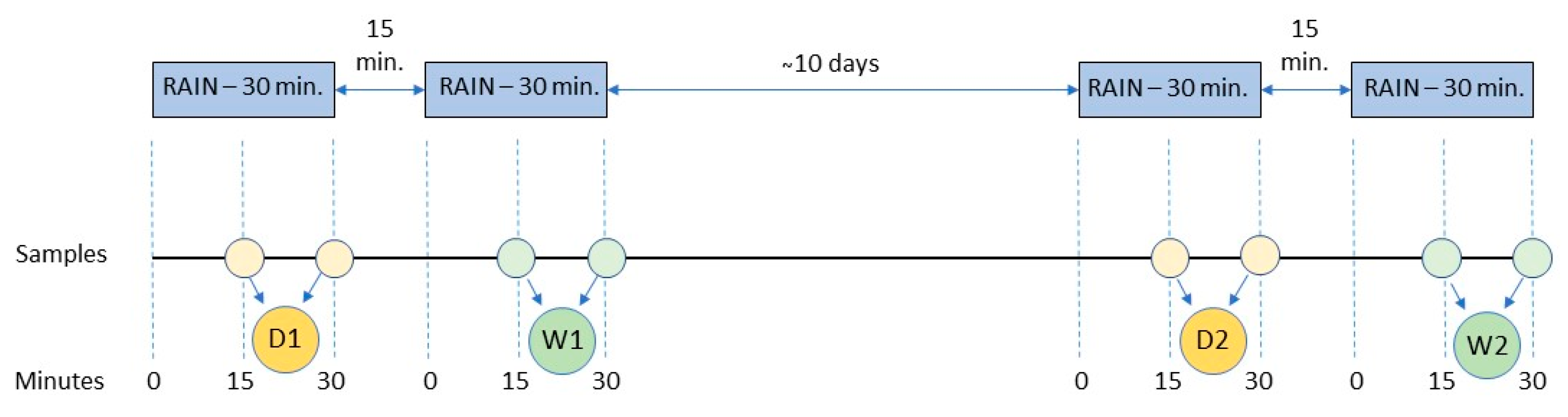
The sampling procedure was as follows (Figure 2). During each experiment, four samples were collected. Two samples were collected during the first experimental rainfall (labelled D1 and W1). The rainfall was divided into two 30 min long rain episodes with a 15 min pause between them without rain. For the next ten days, the container was kept away from the rainfall. The same sampling procedure as in the first part of the experiment was followed. Thus, the other two samples labelled D2 and W2 were collected (plot now had different initial condition compared to the plot during the first experimental rainfall as the plot already contained erosion rills from the previous episode).
The first initial state D1 corresponds to the conditions when the structure is finished. W1 is the state when the soil profile is fully saturated. After 10 days, the soil in the container dried out to the field capacity. The initial states D2 and W2 represent a repeated event. Erosion rills had occurred already after the first part of the experiment (D1). For each slope, at least 35 soil samples were collected.
2.3. Evaluation of Soil Samples—Particle Size Distribution
To find an optimal method for the particle size distribution measurement for our research, three methods were compared: hydrometer, PARIO Soil Particle Analyzer (METER Group, München, Germany), and laser diffractometer Mastersizer 3000 (Malvern Instruments, Malvern, UK). The hydrometer and the PARIO are indirect gravitational sedimentation methods based on Stokes’ law [45] to determine particle size distribution. PARIO is an automated system which uses ISP method [32,46]. Laser diffractometer Mastersizer 3000 provided by Malvern Panalytical allows an exact evaluation of the samples containing soil aggregates and also samples without soil aggregates. The aggregates were destroyed during the measurement by ultrasound [47,48,49]. The hydrometer and PARIO measurements were supplemented by a sieving method. The methods were tested on five samples. From the comparison of the methods, the laser diffraction was found as the most suitable method for our further research, thus all remaining samples were analyzed only by the LD. By the comparison of the particle and aggregate size distribution, the influence of the following external factors was investigated: initial state and slope of the experimental plots.
2.3.1. Sedimentation Methods
The preparation of the soil samples for the particle size analysis by the hydrometer and the PARIO was identical. In a bosh, 40 g of air-dried soil sediment together with 40 mL of sodium hexametaphosphate was boiled for 15 min. Thus, the soil aggregates were destroyed and the fraction content greater than 100 μm was separated. This fraction was oven dried at 105 °C, sieved, and weighed. Mesh sizes of the sieves were 2000 μm, 1250 μm, 1000 μm, 800 μm, 500 μm, 250 μm, and 100 μm. The suspension of fine particles smaller than 100 μm was filled with distilled water in graduated cylinder to reach the volume of 1000 mL [23,50]. Suspension was analyzed by hydrometer and after that, the same suspension was analyzed by the PARIO.
Analysis by the hydrometer continued with suspension mixing and registering of its temperature. The end of the mixing determined the beginning of the sedimentation process, and the hydrometer was put into the suspension. Hydrometer readings were recorded at intervals of 30 s, 1 min, 2 min, 5 min, 10 min, 25 min, 50 min, 75 min, 2.5 h, 24 h, and 48 h from the beginning of the sedimentation process. Finally, the particle size distribution curves were manually calculated using the hydrometer readings and sieve analysis data [50].
Before the measurement by PARIO, the duration parameter—8 h—and timer for homogenization parameter—60 s—were set in the PARIO Control software. Besides the suspension with the soil sample, the graduated cylinder with distilled water was needed. In both of them, the room temperature was the same. The PARIO device was immersed into the distilled water for ten minutes calibrate to temperature. The suspension with the soil sample was mixed for 60 s and the PARIO device was then moved from the distilled water to the suspension. Automated measurement was begun. It took 8 h, and the temperature and the pressure were recorded every 10 s. While the results from the sieving analysis were manually entered to the software, the particle size distribution curves were automatically calculated [46].
2.3.2. Laser Diffractometer—Mastersizer 3000
The Mastersizer 3000 uses optical model Mie theory, which is recommended by ISO 13320 for particles smaller than 50 μm. Mie theory is based on Maxwell’s electromagnetic field equations and provides solution for the calculation of particle size distribution from light scattering data. To obtain accurate results, which the Malvern software calculates based on the data from the laser diffractometer, information about the analyzed material and dispersion medium (refractive and absorption indices which characterize the passage of light through) must be entered before the measurement starts [49].
Silica (SiO2), which has the most similar properties to soil, was selected as a referential material from the software database. Based on the selected material, the software assigned values for the refractive index, 1.457 [22], and the absorption index, 0.010. Water was selected as a dispersion medium with a refractive index value of 1.33. Adjusted values were in agreement with the user manual [49].
The air dried soil sediment was and thoroughly mixed before the measurement to ensure its representativeness. For 40 s, the background data of distilled water was measured. To a beaker of 550 mL distilled water, the amount of the soil sample (approximately one gram) was added in order to achieve the concentration required by the software (obscuration 10–30%).
The analysis of each sample was set up to run 25 records for 20 s each. Laser beam scattering information was recorded during these measurements. During the first five records, the soil sample with aggregates was analyzed. Then, the ultrasound was manually started. Ryzak et al. [20] adduced that 4 min of ultrasound application is enough to destroy all soil aggregates, and that there is no upper limit whose exceeding could cause breaking of the particles themselves. Accordingly, the time of active ultrasound was set to 320 s. By this time soil aggregates had been destroyed, and the five records after ultrasound were carried out on the soil sample, already without aggregates.
Faé et al. [51] found that only one reading per sample is sufficient. Therefore, for further comparison of the particle size analysis, two curves from analysis of each soil sample were used—the average of the first five (soil with aggregates) and the average of the last five records (soil with already destroyed aggregates).
3. Results
The results obtained by measuring the particle and aggregate size distribution of the soil sediment are represented by the dependency graphs of cumulative volume on particle size distribution. The x-axes of these graphs are displayed in a logarithmic scale.
Three particle size values to evaluate the data were selected: <2 μm, <10 μm, and <50 μm. These boundaries were chosen on the basis of the commonly used soil classification systems according to their particle size. The 2 μm value determined the boundaries of the triangular diagram fractions—NRCS USDA [15]. The 10 μm value is used in the Novak’s classification system to classify the soil type [14]. The 50 μm value is again the boundary of the triangular diagram. The numerical representation of the PSD curves is shown in the tables where the median and standard deviation (SD) values for particles smaller than 2 μm, 10 μm, and 50 μm are presented.
3.1. Comparison of Three Tested Methods
The PSD curves of five randomly selected samples (Samples 1–5) obtained by all three methods are shown in Figure 3. In Appendix A, Table A1, Table A2 and Table A3 show the representation of the particles smaller than 2, 10, and 50 μm for all particle size curves obtained by the compared methods. The representation of particles smaller than 2, 10, and 50 μm were averaged and compared in Table 1. Overall, the least differences are between the results from the laser diffractometer and the PARIO, especially the results for the fraction content smaller than 2 μm are very similar (difference 6%). Sedimentation methods are close to each other in fraction content smaller than 50 μm (difference 4%), but comparing both of them to the laser diffractometer there were large differences (18% and 14%) for this fraction. Results for the fraction content smaller than 2 μm obtained by the hydrometer differ significantly compared to those from the laser diffractometer (by 22%) and PARIO (by 16%). The comparison showed that the volume representation of the fraction smaller than 2 μm measured by the laser diffractometer was generally lower than the volume representation analyzed by hydrometer (by 22%) and PARIO (by 6%). On the other hand, the fraction content smaller than 50 μm s lower for the sedimentation methods (by 18% and 14%).
3.2. Samples with and without Soil Aggregates
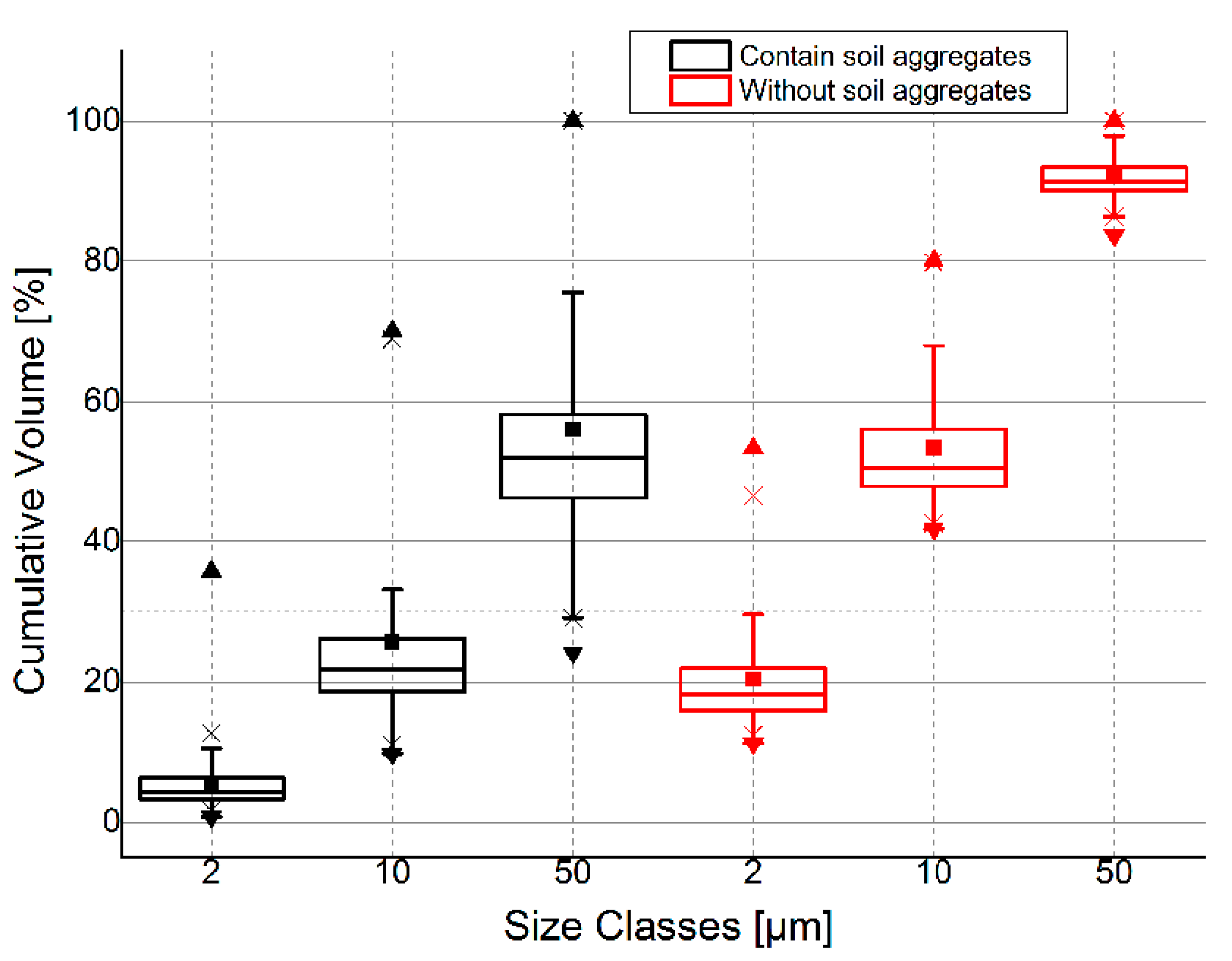
At the beginning, all data were first analyzed in terms of the number of particles that form soil aggregates, independently of other variables. Graphical representation of statistical analysis of PSD of all 156 collected samples is shown in Appendix A in Figure A1.
Table 2 shows all measured particle and aggregate size distribution analysis of 156 soil samples collected from experimental location with and without aggregates. The table shows that the samples, after destruction of the soil aggregates, contain finer particles compared to the samples before destruction of the aggregates, and that the particle size distribution curves after destroying aggregates for particles smaller than 10 and 50 μm have smaller standard deviation than those before its destruction—the SD for particles smaller than 10 and 50 μm was 8.4 and 3.4 for samples without soil aggregates and 13.1 and 16.7 for samples with aggregates, respectively. Graphical representation of statistical analysis of PSD of all 156 collected samples is shown in Appendix A in Figure A1.
3.3. Influence of Initial Condition and Slopes of the Experimental Plots
Table 3, Table 4 and Table 5 show statistical analysis of particle size distribution curves for each slope separately. Graphical representation of these tables is shown in Appendix A in Figure A1. A table representing average statistical analysis of all three slopes is shown in Appendix A (Table A4). The SD of the particle size distribution curves before destroying aggregates was generally higher—the highest for the particles with aggregates smaller than 50 μm (SD of the particles smaller than 50 μm from the slope of 22°—5.8, 9.3, 6.8, and 6.9 for samples D1, W1, D2, and W2, respectively) compared to the curves without aggregates.
For the samples with aggregates from all three slopes, samples D1 and D2 had more particles smaller than 2 μm compared to the samples W1 and W2. The representation of the particles smaller than 10 μm had the same trend. At slopes of 22° and 30°, the representation of particles smaller than 50 μm for samples with aggregates became higher with later sampling time, with the exception of the samples eroded last, W2.
For the samples without aggregates from the slopes of 22° and 30°, samples D1 and D2 had more particles smaller than 2 μm compared to the samples W1 and W2; representation of the particles smaller than 10 μm had also the same trend. For the samples without aggregates eroded from the 34° slope, the representation of the particles smaller than 2 and 10 μm became lower with later sampling time. For the slopes of 30° and 34°, samples D1 and D2 without aggregates had more particles smaller than 50 μm compared to the samples W1 and W2.
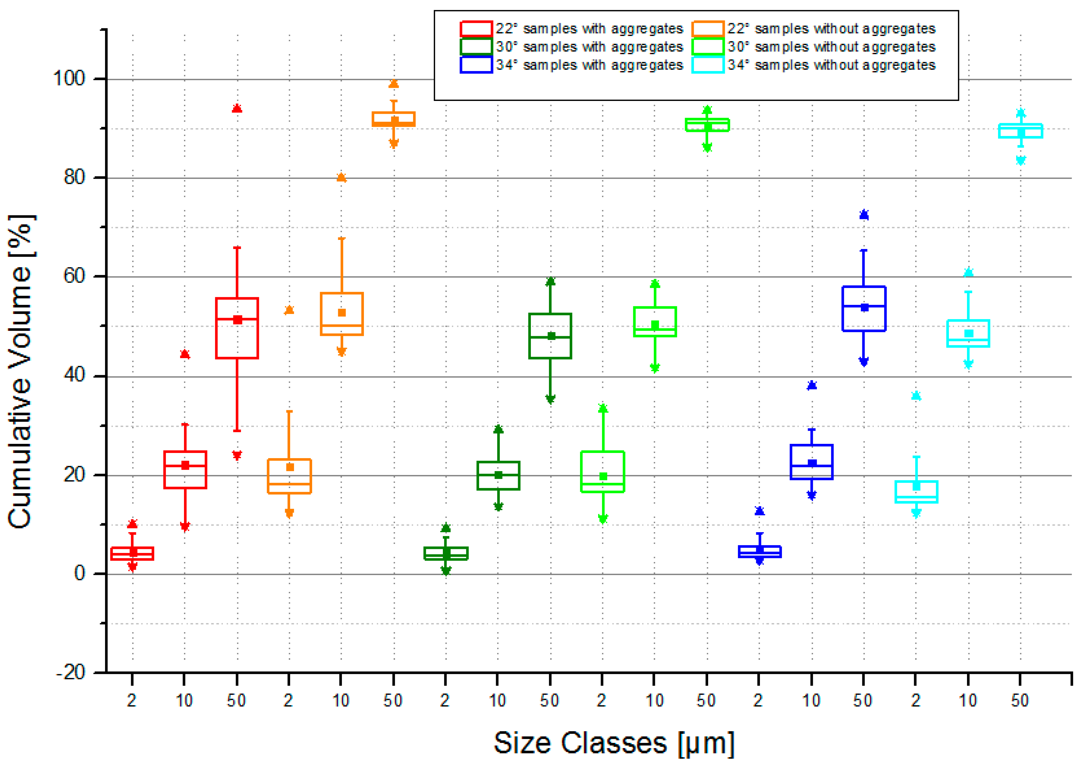
The influence of the slope of the soil container on the aggregate representation percentage in the soil sediment was examined. Graphical representation of statistical analysis of PSD of samples collected from each slope is shown in Appendix A in Figure A2. Table 3, Table 4 and Table 5, the tables representing difference of the median values with and without aggregates for each fraction size were created (Table A6, Table A7 and Table A8). The difference shows aggregate representation percentage in the sample. It is shown that with a later sampling time the median values of aggregate representation decreased on the 30°and 34° slopes and increased on the 22° slope. Furthermore, for particles smaller than 2 and 10 μm, the largest differences during the first part of the experiments (D1 and W1) had samples eroded from the slope 30° (18.8%, 14.1%, 34.0%, and 29.1%, respectively), while during the second part (D2 and W2) it was the samples from the 22° slope (13.0%, 14.3% and 28.4%, 29.8%, respectively). For the particles smaller than 50 μm, the samples from the slope 34° exhibited the least differences (38.0%, 37.1%, 35.0%, and 36.1% for samples D1, W1, D2, and W2, respectively) and the samples from the slope 30° the largest differences (45.5%, 43.1%, 43.7%, and 42.0% for samples D1, W1, D2, and W2, respectively).
4. Discussion
The research presented here had two main goals. The first one was to determine the limits of using the methods to analyze PSD for estimation the intensity of the erosion process on artificial slopes. The second goal was the actual analysis of the PSD and aggregate percentage representation of eroded soil samples in relation to external factors (slope, initial soil water content).
4.1. Comparison of Three Tested Methods
From the mutual comparison of the three methods tested, it is obvious that the results from the hydrometer are overestimated compared to the other two methods and suggest that the number of particles finer than 1 μm is almost 40% in all tested soil samples, which corresponds to the PSD analysis of the original soil. The shape of the particle size distribution curves obtained by the PARIO is similar to those from laser diffractometer, while the curves with a linear trend obtained from the hydrometer differ; see Figure 3.
The representation of particles smaller than 2, 10, and 50 μm were compared in Table 1. It was found that the fraction smaller than 2 μm obtained by the LD was lower compared to the sedimentation method, and the fraction smaller than 50 μm had an opposite result. This confirms the conclusions from the previous studies [21,23,27,28,29,30,31] which state that the laser diffraction underestimates the clay fraction content and overestimates the silt fraction content. Furthermore, it was found that LD and hydrometer gave very similar results for particle size <10 μm. Note that this value is a boundary used in the Novak’s classification system [14].
The time required for the methods tested varies greatly. To determine the PSD using both the hydrometer and the PARIO, the standard sample preparation is required before the measurement to destroy soil aggregates and separate the fine fraction from the sand fraction. This preparation takes about 25 min per sample. In addition, a sieve analysis required for the sand fraction of each sample takes another 10 min. The hydrometer measurement takes 48 h and the PARIO measurement takes 8 h for one sample. However, in 2021 the METER Group developed the innovative device PARIO Plus which can reduce the analysis time to 2.5 h [46]. The PSD analysis by the LD requires no prior preparation of the soil sample except for thorough mixing. The particle size distribution is analyzed for 15 min per sample. Evaluation of the PSD of all 156 samples by LD took 39 h. If the PARIO was used for the particle size analysis of all samples, the total measurement time would be 340 h and the hydrometer evaluation would take 1590 h, i.e., more than 66 days (if five PARIO devices and five hydrometers were used).
The main advantage of using of the laser diffractometer is that the soil aggregates are destroyed during the measurement by ultrasound which is sufficient and a very time and user-friendly method [20]. Also, the particle size can be analyzed before the aggregates are destroyed. Such results are satisfying thanks to the principles of laser diffraction. On the other hand, the sample preparation for the hydrometer and PARIO measurements is demanding and analysis of the soil samples with aggregates using sedimentations principles (Stokes’ law) has physical imperfections.
A significant advantage of the laser diffractometer’s particle size analysis is the amount of sample that is required for evaluation—while the weight of the soil sample for both sedimentation methods must be at least 50 g, for the laser diffractometer, about 1 g of material is sufficient. This advantage is beneficial, especially when the amount of eroded sediment is small and, in some cases, it could be even less than 50 g. On the other hand, the small amount of the material can decrease representativeness of the whole sample during the measurement.
4.2. Influence of External Factors to the Particle Size Distribution
Graphical representation of statistical analysis of PSD of all 156 collected samples is shown in Appendix A in Figure A1.
Table 2 shows comparison of samples with and without aggregates. The volume of particles larger than 50 μm was almost 50% in soil with aggregates, while it was 10% in the soil without aggregates. The number of particles smaller than 2 μm was less than 5% in the sediment with aggregates and 18% in the soil without aggregates. This means that the particles before using ultrasound were coarser than those analyzed after its use. This proves that the eroded soil is clustered into the soil aggregates [18]. As the table presents all samples which were collected under different conditions (slope, initial condition), the particle size distribution curves of the samples without aggregates had less SD and were more consist than those with aggregates. If the results with aggregates are divided into each slope separately (Table 3, Table 4 and Table 5), the SD is much smaller compared to all samples together (for samples without aggregates the difference in SD is not so significant). This is because the PSD with aggregates depends more on the external conditions (slope) than the size of the soil particles that are forming the aggregates. This fact is the motivation for our further research.
Influence of initial condition and slopes of the experimental plots was analyzed. Hao et al. [40] found that the sediment washed out during rill erosion is formed by coarser particles compared to the sediment eroded at the beginning of the rain during sheet flow. In our research, we found (Table 3, Table 4 and Table 5) that samples eroded as a dry variant (D1 and D2) contained more particles in fraction <2 and <10 μm compared to those eroded as a wet variant (W1 and W2). This could mean that at the beginning of the experiment the sheet flow is present, then the runoff was stabilized and the rill erosion occurred. After ten days without rain, at the beginning of the second part of the experiment (D2), the eroded samples contained more particles in fraction <2 and <10 μm than the W1 sample, even though the erosion rills were already made. The number of particles smaller than 50 μm increased over the sampling time. This means that in general, the eroded particles became finer throughout the experiments.
Table A6, Table A7 and Table A8 show the percentage representation of the aggregates calculated as the difference between the median values. The smaller the difference, the less aggregate representation percentage the sample contains. The soil sediment eroded at the beginning of the rain from the steep slopes contained more aggregates compared to the sediment eroded later. However, in the plot with the slope 22° this trend was the opposite.
If the aggregate representation percentage in fraction smaller than 2 μm is subtracted from the fraction smaller than 10 μm, the fraction content 2–10 μm is obtained. Such values had almost the same percentage representation of particles for all three slopes (13.6% to 15.9%), thus it is apparent that the main difference was generated by particles smaller than 2 μm.
During the first part of the experiment (when the erosion rills were forming—D1 and W1), the largest percentage representation of aggregates in a sample was eroded from the 30° slope, while during the second part of the experiment (when the erosion rills were already formed—D2 and W2), the largest percentage representation of aggregates was eroded from the 22° slope. The least percentage representation of aggregates was eroded from the 34° slope throughout the experiment. The percentage representation of aggregates increased for the 22° slope and decreased for the 30° and 34° slopes throughout the experiment. This means that for steep slopes, the rill erosion was present and only smaller percentage representation of aggregates was eroded.
Samples without soil aggregates contained smaller particles from the 30° slope compared to the 22° slope. However, the particles eroded from the extreme 34° slope gradient used in our research was the finest compared to the less steep slopes. This result agrees with Shanshan et al. [33], who concluded that on the steep slopes (higher than 25°) the erosion processes decrease.
5. Conclusions
During our research, it was found that the method that uses the rainfall simulators where the eroded sediment is collected and then analyzed by laser diffraction to obtain the particle size distribution data is a suitable method to evaluate the impact of the external factors to the particle size distribution of the eroded soil sediment.
The main advantages of the laser diffractometer Mastersizer 3000 compared to the hydrometer and the PARIO are the very short evaluating time of 15 min per sample, the small amount of required sample at 1 g, and its ability to comfortably and relevantly analyze soil samples both with and without soil aggregates.
When the soil is fully saturated and the erosion rills are made, the samples contained coarser particles than the samples eroded during the sheet flow. Also, in general, the eroded particles had become finer throughout the experiments.
Generally, when the erosion processes were intensive (steep slope or long duration of the raining), the eroded sediment contained coarser particles and lower amounts of the aggregates.
For further research, it would be interesting to study aggregates content on more samples obtained from plots with different soil types or with different rainfall intensities, and also to analyze PSD results in the context of volume of the surface runoff and the formation of the rills.
Author Contributions
Conceptualization, R.K. and P.K.; Data curation, M.N. and P.K.; Formal analysis, R.K.; Investigation, R.K.; Methodology, R.K., M.N. and P.K.; Software, M.N.; Supervision, P.K.; Writing—original draft, R.K.; Writing—review & editing, M.N. and P.K. All authors have read and agreed to the published version of the manuscript.
Funding
This research was funded by the TH02030428—“Design of technical measures for slopes stabilization and soil erosion prevention”. And by the international CTU grant SGS20/156/OHK1/3T/11.
Institutional Review Board Statement
The study was conducted according to the guidelines of the Declaration of Helsinki, and approved by the Institutional Review Board (or Ethics Committee) of CTU in Prague.
Informed Consent Statement
Informed consent was obtained from all subjects involved in the study.
Data Availability Statement
The data that support the findings of this study are available on request from the corresponding author.
Conflicts of Interest
The authors declare no conflict of interest and the funders had no role in the design of the study; in the collection, analyses, or interpretation of data; in the writing of the manuscript, or in the decision to publish the results.
Appendix A

Table A1.
Representation of the particles smaller than 2 μm obtained by three tested methods.
| LD | Hydrometer | PARIO | |
|---|---|---|---|
| Sample 1 | 26% | 40% | 16% |
| Sample 2 | 10% | 42% | 19% |
| Sample 3 | 12% | 41% | 29% |
| Sample 4 | 16% | 43% | 22% |
| Sample 5 | 33% | 42% | 40% |
Table A2.
Representation of the particles smaller than 10 μm obtained by three tested methods.
| LD | Hydrometer | PARIO | |
|---|---|---|---|
| Sample 1 | 56% | 51% | 29% |
| Sample 2 | 42% | 53% | 32% |
| Sample 3 | 42% | 53% | 41% |
| Sample 4 | 50% | 56% | 34% |
| Sample 5 | 59% | 57% | 57% |
Table A3.
Representation of the particles smaller than 50 μm obtained by three tested methods.
| LD | Hydrometer | PARIO | |
|---|---|---|---|
| Sample 1 | 91% | 70% | 70% |
| Sample 2 | 88% | 70% | 75% |
| Sample 3 | 86% | 71% | 79% |
| Sample 4 | 92% | 72% | 80% |
| Sample 5 | 91% | 74% | 73% |
Table A4.
Median values of PSD of samples with and without aggregates on all slopes together and each slope separately (obtained by LD) [%].
Table A4.
Median values of PSD of samples with and without aggregates on all slopes together and each slope separately (obtained by LD) [%].
| with Aggregates | without Aggregates | ||
|---|---|---|---|
| all | <2 μm | 4.3 | 18.2 |
| <10 μm | 21.7 | 50.5 | |
| <50 μm | 52.0 | 91.3 | |
| 22° | <2 μm | 4.2 | 17.4 |
| <10 μm | 21.0 | 49.4 | |
| <50 μm | 50.6 | 91.2 | |
| 30° | <2 μm | 4.2 | 19.1 |
| <10 μm | 20.5 | 50.2 | |
| <50 μm | 47.7 | 91.3 | |
| 34° | <2 μm | 4.4 | 16.4 |
| <10 μm | 21.6 | 48.4 | |
| <50 μm | 53.5 | 90.1 |
Figure A1.
LD method. Boxplot representation of PSD of all 156 collected samples with and without soil aggregates.
Figure A1.
LD method. Boxplot representation of PSD of all 156 collected samples with and without soil aggregates.

Table A5.
Statistical analysis of influence of initial conditions to the particle size distribution (obtained by LD) [%] (average of all three slopes).
Table A5.
Statistical analysis of influence of initial conditions to the particle size distribution (obtained by LD) [%] (average of all three slopes).
| with Aggregates | without Aggregates | ||||||||
|---|---|---|---|---|---|---|---|---|---|
| D1 | W1 | D2 | W2 | D1 | W1 | D2 | W2 | ||
| Median ± SD | <2 μm | 4.8 ± 1.6 | 3.6 ± 1.8 | 4.9 ± 2.1 | 3.6 ± 1.4 | 20.1 ± 4.3 | 16.6 ± 5.6 | 17.5 ± 4.6 | 16.4 ± 5.2 |
| <10 μm | 21.9 ± 3.3 | 20.0 ± 4.6 | 22.1 ± 4.9 | 20.2 ± 3.8 | 52.0 ± 3.0 | 48.4 ± 4.3 | 48.9 ± 3.3 | 48.0 ± 3.7 | |
| <50 μm | 50.0 ± 4.9 | 50.6 ± 8.7 | 51.8 ± 6.4 | 50.0 ± 5.5 | 91.5 ± 1.4 | 90.6 ± 1.8 | 90.8 ± 1.2 | 90.5 ± 1.8 | |
Table A6.
Aggregate representation percentage in the sediment depending on initial condition, slope 22° [%].
Table A6.
Aggregate representation percentage in the sediment depending on initial condition, slope 22° [%].
| D1 | W1 | D2 | W2 | |
|---|---|---|---|---|
| <2 μm | 12.8 | 12.8 | 13.0 | 14.3 |
| <10 μm | 27.2 | 28.2 | 28.4 | 29.8 |
| <50 μm | 40.8 | 39.6 | 38.5 | 43.3 |
Table A7.
Aggregate representation percentage in the sediment depending on initial condition, slope 30° [%].
Table A7.
Aggregate representation percentage in the sediment depending on initial condition, slope 30° [%].
| D1 | W1 | D2 | W2 | |
|---|---|---|---|---|
| <2 μm | 18.8 | 14.1 | 13.5 | 13.0 |
| <10 μm | 34.0 | 29.1 | 27.3 | 28.2 |
| <50 μm | 45.5 | 43.1 | 43.7 | 42.0 |
Table A8.
Aggregate representation percentage in the sediment depending on initial condition, slope 34° [%].
Table A8.
Aggregate representation percentage in the sediment depending on initial condition, slope 34° [%].
| D1 | W1 | D2 | W2 | |
|---|---|---|---|---|
| <2 μm | 14.3 | 11.9 | 11.0 | 11.1 |
| <10 μm | 29.1 | 27.8 | 24.6 | 25.5 |
| <50 μm | 38.0 | 37.1 | 35.0 | 36.1 |
Figure A2.
Boxplot representation of influence of slope of the experimental plot to the PSD (obtained by LD).
Figure A2.
Boxplot representation of influence of slope of the experimental plot to the PSD (obtained by LD).

References
- Toy, T.J.; Foster, G.R.; Renard, K.G. Soil Erosion: Processes, Prediction, Measurement, and Control; John JWS: New York, NY, USA, 2002. [Google Scholar]
- Slattery, M.C.; Burt, T.P. Particle size characteristics of suspended sediment in hillslope runoff and stream flow. Earth Surf. Process. Landf. 1997, 22, 705–719. [Google Scholar] [CrossRef]
- Benaud, P.; Anderson, K.; Evans, M.; Farrow, L.; Glendell, M.; James, M.R.; Quine, T.A.; Quinton, J.N.; Rawlins, B.; Jane Rickson, R.; et al. National-scale geodata describe widespread accelerated soil erosion. Geoderma 2020, 371, 114378. [Google Scholar] [CrossRef]
- Biddoccu, M.; Zecca, O.; Audisio, C.; Godone, F.; Barmaz, A.; Cavallo, E. Assessment of Long-Term Soil Erosion in a Mountain Vineyard, Aosta Valley (NW Italy). Land Degrad. Dev. 2018, 29, 617–629. [Google Scholar] [CrossRef]
- Brazier, R.E.; Bilotta, G.S.; Haygarth, P.M. A perspective on the role of lowland, agricultural grasslands in contributing to erosion and water quality problems in the UK. Earth Surf. Process. Landf. 2007, 32, 964–967. [Google Scholar] [CrossRef]
- Grand-Clement, E.; Luscombe, D.J.; Anderson, K.; Gatis, N.; Benaud, P.; Brazier, R.E. Antecedent conditions control carbon loss and downstream water quality from shallow, damaged peatlands. Sci. Total Environ. 2014, 493, 961–973. [Google Scholar] [CrossRef] [Green Version]
- Guo, Y.; Peng, C.; Zhu, Q.; Wang, M.; Wang, H.; Peng, S.; He, H. Modelling the impacts of climate and land use changes on soil water erosion: Model applications, limitations and future challenges. J. Environ. Manag. 2019, 250, 109403. [Google Scholar] [CrossRef]
- Montgomery, D.R. Soil erosion and agricultural sustainability. Proc. Natl. Acad. Sci. USA 2007, 104, 13268–13272. [Google Scholar] [CrossRef] [Green Version]
- Pimentel, D. Soil erosion: A food and environmental threat. Environ. Dev. Sustain. 2006, 8, 119–137. [Google Scholar] [CrossRef]
- Singer, M.J.; Warkentin, B.P. Soils in an environmental context: An American perspective. Catena 1996, 27, 179–189. [Google Scholar] [CrossRef]
- Sun, W.; Shao, Q.; Liu, J. Soil erosion and its response to the changes of precipitation and vegetation cover on the Loess Plateau. J. Geogr. Sci. 2013, 23, 1091–1106. [Google Scholar] [CrossRef]
- Day, P.R. Particle fractionation and particle-size analysis. In Methods of Soil Analysis; ASA: Alexandria, VA, USA, 1965. [Google Scholar]
- Zádorová, T.; Penížek, V. Problems in correlation of Czech national soil classification and World Reference Base 2006. Geoderma 2011, 167–168, 54–60. [Google Scholar] [CrossRef]
- Soil Survey Staff. Keys to Soil Taxonomy, 12th ed.; USDA-Natural Resources Conservation Service: Washington, DC, USA, 2014.
- American Society for Testing and Materials. Classification of Soils for Engineering Purposes: Annual Book of ASTM Standards, D 2487-83, 04; American Society for Testing and Materials: West Conshohocken, PA, USA, 1985; pp. 395–408. [Google Scholar]
- Carminati, A.; Kaestner, A.; Hassanein, R.; Ippisch, O.; Vontobel, P.; Flühler, H. Infiltration through series of soil aggregates: Neutron radiography and modeling. Adv. Water Resour. 2007, 30, 1168–1178. [Google Scholar] [CrossRef]
- Zemědělci, V. Příručka Ochrany Proti Vodní Erozi; Ministerstvo zemědělství: Praha, Czech Republic, 2014. [Google Scholar]
- Zumr, D.; Jeřábek, J.; Klípa, V.; Dohnal, M.; Sněhota, M. Estimates of tillage and rainfall effects on unsaturated hydraulic conductivity in a small central european agricultural catchment. Water 2019, 11, 740. [Google Scholar] [CrossRef] [Green Version]
- Bieganowski, A.; Zaleski, T.; Kajdas, B.; Sochan, A.; Józefowska, A.; Beczek, M.; Lipiec, J.; Turski, M.; Ryżak, M. An improved method for determination of aggregate stability using laser diffraction. Land Degrad. Dev. 2018, 29, 1376–1384. [Google Scholar] [CrossRef]
- Ryzak, M.; Bieganowski, A. Methodological aspects of determining soil particle-size distribution using the laser diffraction method. J. Plant Nutr. Soil Sci. 2011, 174, 624–633. [Google Scholar] [CrossRef]
- Eshel, G.; Levy, G.J.; Mingelgrin, U.; Singer, M.J. Critical evaluation of the use of laser diffraction for particle-size distribution analysis. Soil Sci. Soc. Am. J. 2004, 68, 736–743. [Google Scholar] [CrossRef]
- Arriaga, F.J.; Lowery, B.; Mays, D.W. A fast method for determining soil particle size distribution using a laser instruments. Soil Sci. 2006, 171, 663–674. [Google Scholar] [CrossRef] [Green Version]
- Beuselinck, L.; Govers, G.; Poesen, J.; Degraer, G.; Froyen, L. Grain-size analysis by laser diffractometry: Comparison with the sieve-pipette method. Catena 1998, 32, 193–208. [Google Scholar] [CrossRef]
- Kimura, S.; Ito, T.; Minagawa, H. Grain-size analysis of fine and coarse non-plastic grains: Comparison of different analysis methods. Granul. Matter 2018, 20, 1–15. [Google Scholar] [CrossRef]
- Konert, M.; Vandenberghe, J. Comparison of laser grain size analysis with pipette and sieve analysis: A solution for the underestimation of the clay fraction. Sedimentology 1997, 44, 523–535. [Google Scholar] [CrossRef] [Green Version]
- Lamorski, K.; Bieganowski, A.; Ryzak, M.; Sochan, A.; Sławiński, C.; Stelmach, W. Assessment of the usefulness of particle size distribution measured by laser diffraction for soil water retention modelling. J. Plant Nutr. Soil Sci. 2014, 177, 803–813. [Google Scholar] [CrossRef]
- Pieri, L.; Bittelli, M.; Pisa, P.R. Laser diffraction, transmission electron microscopy and image analysis to evaluate a bimodal Gaussian model for particle size distribution in soils. Geoderma 2006, 135, 118–132. [Google Scholar] [CrossRef]
- Vdović, N.; Obhođaš, J.; Pikelj, K. Revisiting the particle-size distribution of soils: Comparison of different methods and sample pre-treatments. Eur. J. Soil Sci. 2010, 61, 854–864. [Google Scholar] [CrossRef]
- Di Stefano, C.; Ferro, V.; Mirabile, S. Comparison between grain-size analyses using laser diffraction and sedimentation methods. Biosyst. Eng. 2010, 106, 205–215. [Google Scholar] [CrossRef]
- Igaz, D.; Aydin, E.; Šinkovičová, M.; Šimanský, V.; Tall, A.; Horák, J. Laser diffraction as an innovative alternative to standard pipette method for determination of soil texture classes in central europe. Water 2020, 12, 1232. [Google Scholar] [CrossRef]
- Mattheus, C.R.; Diggins, T.P.; Santoro, J.A. Issues with integrating carbonate sand texture data generated by different analytical approaches: A comparison of standard sieve and laser-diffraction methods. Sediment. Geol. 2020, 401, 105635. [Google Scholar] [CrossRef]
- Durner, W.; Iden, S.C.; von Unold, G. The integral suspension pressure method (ISP) for precise particle-size analysis by gravitational sedimentation. Water Resour. Res. 2017, 53, 33–48. [Google Scholar] [CrossRef]
- Shanshan, W.; Baoyang, S.; Chaodong, L.; Zhanbin, L.; Bo, M. Runoff and Soil Erosion on Slope Cropland: A Review. JRE 2018, 12, 461–470. [Google Scholar] [CrossRef]
- Jing, X.; Chen, Y.; Pan, C.; Yin, T.; Wang, W.; Fan, X. Erosion failure of a soil slope by heavy rain: Laboratory investigation and modified GA model of soil slope failure. Int. J. Environ. Res. Public Health 2019, 16, 1075. [Google Scholar] [CrossRef] [Green Version]
- Bissonnais, Y. Aggregate stability and assessment of soil crustability and erodibility: I. Theory and methodology. Eur. J. Soil Sci. 1996, 47, 425–437. [Google Scholar] [CrossRef]
- Kasmerchaka, C.S.; Mason, J.A.; Liang, M. Laser diffraction analysis of aggregate stability and disintegration in forest and grassland soils of northern Minnesota, USA. Geoderma 2019, 338, 430–444. [Google Scholar] [CrossRef]
- Asadi, H.; Moussavi, A.; Ghadiri, H.; Rose, C.W. Flow-driven soil erosion processes and the size selectivity of sediment. J. Hydrol. 2011, 406, 73–81. [Google Scholar] [CrossRef] [Green Version]
- Quan, X.; He, J.; Cai, Q.; Sun, L.; Li, X.; Wang, S. Soil erosion and deposition characteristics of slope surfaces for two loess soils using indoor simulated rainfall experiment. Soil Tillage Res. 2020, 204, 104714. [Google Scholar] [CrossRef]
- Wei, S.; Zhang, X.; McLaughlin, N.B.; Chen, X.; Jia, S.; Liang, A. Impact of soil water erosion processes on catchment export of soil aggregates and associated SOC. Geoderma 2017, 294, 63–69. [Google Scholar] [CrossRef]
- Hao, H.; Wang, X.; Guang, J.; Guo, Z.; Hua, L. Water erosion processes and dynamic changes of sediment size distribution under the combined effects of rainfall and overland flow. Catena 2019, 173, 494–504. [Google Scholar] [CrossRef]
- Vaníček, M.; Vaníček, J.; Kavka, P.; Zumr, D.; Marek, O. Efficiency of erosion prevention geosynthetics for non-vegetated slopes during extreme artificial rainfalls testing. In Proceedings of the XVII European Conference on Soil Mechanics and Geotechnical Engineering, Reykjavik, Iceland, 1–6 September 2019. [Google Scholar]
- Kavka, P.; Neumann, M.; Laburda, T.; Zumr, D. Developing of the laboratory rainfall simulator for testing the technical soil surface protection measures and droplets impact. In Proceedings of the XVII European Conference on Soil Mechanics and Geotechnical Engineering, Reykjavik, Iceland, 1–6 September 2019. [Google Scholar]
- Kavka, P.; Neumann, M. Swinging-Pulse Sprinkling Head for Rain Simulators. Hydrology 2021, 8, 74. [Google Scholar] [CrossRef]
- Úřad Pro Technickou Normalizaci, Metrologii a Státní Zkušebnictví. ČSN 73 6133. Návrh a Provádění Zemního Tělesa Pozemních Komunikací: Road Earthwork—Design and Execution; Úřad Pro Technickou Normalizaci, Metrologii a Státní Zkušebnictví: Praha, Czech Republic, 2010. [Google Scholar]
- Stokes, G.G. On the effect of the internal friction of fluids on the motion of pendulums. Trans. Camb. Philos. Soc. 1850, IX, 1–86. [Google Scholar]
- METER Group. PARIO Soil Particle Analyzer—Manual; METER Group: München, Germany, 2018. [Google Scholar]
- Ghasemy, A.; Rahimi, E.; Malekzadeh, A. Introduction of a new method for determining the particle-size distribution of fine-grained soils. Meas. J. Int. Meas. Confed. 2019, 132, 79–86. [Google Scholar] [CrossRef]
- Malvern Instruments Ltd. Mastersizer 2000 User Manual; Malvern Instruments Ltd.: Malvern, UK, 2007. [Google Scholar]
- Malvern Instruments Ltd. Mastersizer 3000 User Manual; Malvern Instruments Ltd.: Malvern, UK, 2017. [Google Scholar]
- Motsara, M.R.; Roy, R.N. Guide to Laboratory Establishment for Plant Nutrient Analysis; Food and Agriculture Organization of the United Nations: Rome, Italy, 2008. [Google Scholar]
- Faé, G.S.; Montes, F.; Bazilevskaya, E.; Añó, R.M.; Kemanian, A.R. Making Soil Particle Size Analysis by Laser Diffraction Compatible with Standard Soil Texture Determination Methods. Soil Sci. Soc. Am. J. 2019, 83, 1244–1252. [Google Scholar] [CrossRef] [Green Version]
Figure 1.
Experimental plots. Slope 34°, 30° and 22°. Dimensions 4.25 × 1 × 1.6 m. Rainfall simulator pulse nozzle system type WSQ 40. Location–Jirkov.
Figure 1.
Experimental plots. Slope 34°, 30° and 22°. Dimensions 4.25 × 1 × 1.6 m. Rainfall simulator pulse nozzle system type WSQ 40. Location–Jirkov.

Figure 2.
Scheme of the sampling procedure at the experimental plots.

Figure 3.
Comparison of PSD curves of soil samples measured by three tested methods–LD (black, solid), hydrometer (red, dashed) and PARIO (blue, dotted): (a) Sample 1; (b) Sample 2; (c) Sample; (d) Sample 4; (e) Sample 5.
Figure 3.
Comparison of PSD curves of soil samples measured by three tested methods–LD (black, solid), hydrometer (red, dashed) and PARIO (blue, dotted): (a) Sample 1; (b) Sample 2; (c) Sample; (d) Sample 4; (e) Sample 5.

Table 1.
Comparison of average differences of representation of particles smaller than 2, 10 and 50 μm between three tested methods (±SD), differences between the results for methods in the first and the last column.
Table 1.
Comparison of average differences of representation of particles smaller than 2, 10 and 50 μm between three tested methods (±SD), differences between the results for methods in the first and the last column.
| Method | <2 μm | <10 μm | <50 μm | Method |
|---|---|---|---|---|
| LD | −22 ± 9% | −4 ± 7% | 18 ± 2% | Hydrometer |
| LD | −6 ± 9% | 11 ± 10% | 14 ± 5% | PARIO |
| PARIO | 16 ± 8% | 15 ± 9% | −4 ± 4% | Hydrometer |
Table 2.
LD method. Statistical analysis (median and standard deviation) of PSD of all 156 collected samples [%].
Table 2.
LD method. Statistical analysis (median and standard deviation) of PSD of all 156 collected samples [%].
| With Aggregates | Without Aggregates | ||
|---|---|---|---|
| Median ± SD | <2 μm | 4.3 ± 3.5 | 18.2 ± 6.9 |
| <10 μm | 21.7 ± 13.1 | 50.5 ± 8.4 | |
| <50 μm | 52.0 ± 16.7 | 91.3 ± 3.4 |
Table 3.
Statistical analysis (median and standard deviation) of influence of initial conditions to the particle size distribution (obtained by LD) for the samples from the plot with slope 22° [%].
Table 3.
Statistical analysis (median and standard deviation) of influence of initial conditions to the particle size distribution (obtained by LD) for the samples from the plot with slope 22° [%].
| With Aggregates | Without Aggregates | ||||||||
|---|---|---|---|---|---|---|---|---|---|
| D1 | W1 | D2 | W2 | D1 | W1 | D2 | W2 | ||
| Median ± SD | <2 μm | 5.2 ± 1.5 | 3.5 ± 1.7 | 5.0 ± 2.5 | 3.0 ± 1.3 | 17.9 ± 1.9 | 16.2 ± 7.7 | 18.0 ± 3.8 | 17.3 ± 7.0 |
| <10 μm | 22.4 ± 4.0 | 20.1 ± 4.3 | 22.0 ± 5.4 | 19.3 ± 4.5 | 49.6 ± 1.3 | 48.4 ± 5.0 | 50.5 ± 2.9 | 49.1 ± 4.6 | |
| <50 μm | 50.5 ± 5.8 | 51.7 ± 9.3 | 52.4 ± 6.8 | 47.8 ± 6.9 | 91.3 ± 1.1 | 91.3 ± 1.9 | 90.9 ± 1.2 | 91.1 ± 1.0 | |
Table 4.
Statistical analysis (median and standard deviation) of influence of initial conditions to the particle size distribution (obtained by LD) for the samples from the plot with slope 30° [%].
Table 4.
Statistical analysis (median and standard deviation) of influence of initial conditions to the particle size distribution (obtained by LD) for the samples from the plot with slope 30° [%].
| With Aggregates | Without Aggregates | ||||||||
|---|---|---|---|---|---|---|---|---|---|
| D1 | W1 | D2 | W2 | D1 | W1 | D2 | W2 | ||
| Median ± SD | <2 μm | 4.0 ± 1.8 | 3.5 ± 0.9 | 5.5 ± 1.9 | 3.9 ± 1.7 | 22.8 ± 4.2 | 17.5 ± 6.6 | 19.0 ± 3.7 | 16.9 ± 4.0 |
| <10 μm | 20.3 ± 2.3 | 19.5 ± 3.0 | 22.4 ± 4.7 | 20.0 ± 3.6 | 54.2 ± 3.0 | 48.6 ± 4.7 | 49.7 ± 2.2 | 48.2 ± 2.6 | |
| <50 μm | 46.9 ± 4.6 | 47.5 ± 6.9 | 47.5 ± 6.7 | 49.0 ± 4.5 | 92.4 ± 1.2 | 90.6 ± 1.5 | 91.2 ± 0.9 | 90.9 ± 2.1 | |
Table 5.
Statistical analysis (median and standard deviation) of influence of initial conditions to the particle size distribution (obtained by LD) for the samples from the plot with slope 34° [%].
Table 5.
Statistical analysis (median and standard deviation) of influence of initial conditions to the particle size distribution (obtained by LD) for the samples from the plot with slope 34° [%].
| With Aggregates | Without Aggregates | ||||||||
|---|---|---|---|---|---|---|---|---|---|
| D1 | W1 | D2 | W2 | D1 | W1 | D2 | W2 | ||
| Median ± SD | <2 μm | 5.3 ± 1.6 | 4.0 ± 2.9 | 4.3 ± 2.1 | 3.9 ± 1.1 | 19.5 ± 6.8 | 15.9 ± 2.4 | 15.4 ± 6.4 | 14.9 ± 4.6 |
| <10 μm | 23.0 ± 3.5 | 20.4 ± 6.5 | 21.9 ± 4.6 | 21.2 ± 3.1 | 52.0 ± 4.8 | 48.3 ± 3.1 | 46.5 ± 4.7 | 46.7 ± 3.8 | |
| <50 μm | 52.7 ± 4.2 | 52.7 ± 9.8 | 55.4 ± 5.8 | 53.4 ± 5.2 | 90.7 ± 2.1 | 89.8 ± 1.8 | 90.3 ± 1.5 | 89.5 ± 2.2 | |
Publisher’s Note: MDPI stays neutral with regard to jurisdictional claims in published maps and institutional affiliations. |
© 2021 by the authors. Licensee MDPI, Basel, Switzerland. This article is an open access article distributed under the terms and conditions of the Creative Commons Attribution (CC BY) license (https://creativecommons.org/licenses/by/4.0/).
Share and Cite
MDPI and ACS Style
Kubínová, R.; Neumann, M.; Kavka, P. Aggregate and Particle Size Distribution of the Soil Sediment Eroded on Steep Artificial Slopes. Appl. Sci. 2021, 11, 4427. https://0-doi-org.brum.beds.ac.uk/10.3390/app11104427
AMA Style
Kubínová R, Neumann M, Kavka P. Aggregate and Particle Size Distribution of the Soil Sediment Eroded on Steep Artificial Slopes. Applied Sciences. 2021; 11(10):4427. https://0-doi-org.brum.beds.ac.uk/10.3390/app11104427
Chicago/Turabian StyleKubínová, Romana, Martin Neumann, and Petr Kavka. 2021. "Aggregate and Particle Size Distribution of the Soil Sediment Eroded on Steep Artificial Slopes" Applied Sciences 11, no. 10: 4427. https://0-doi-org.brum.beds.ac.uk/10.3390/app11104427
Note that from the first issue of 2016, this journal uses article numbers instead of page numbers. See further details here.