
Wind-Resistant Capacity Modeling for Electric Transmission Line Towers Using Kriging Surrogates and Its Application to Structural Fragility

Abstract
:Featured Application
Abstract
1. Introduction
2. Tower Capacity
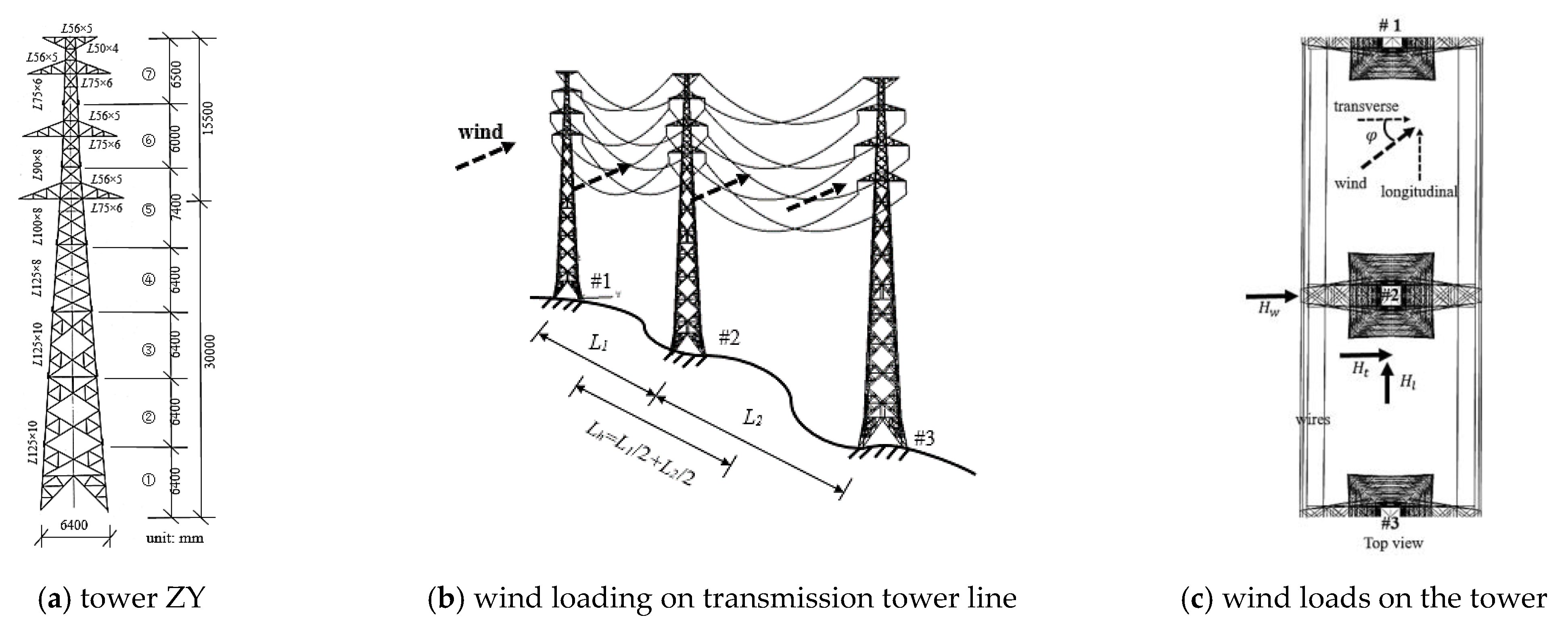
2.1. Wind Loading
2.2. Limit Capacity
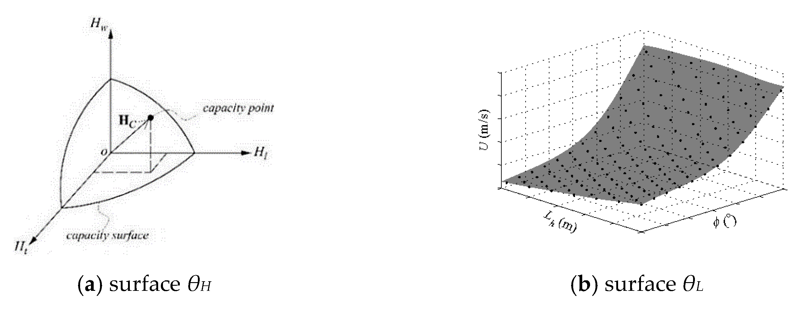
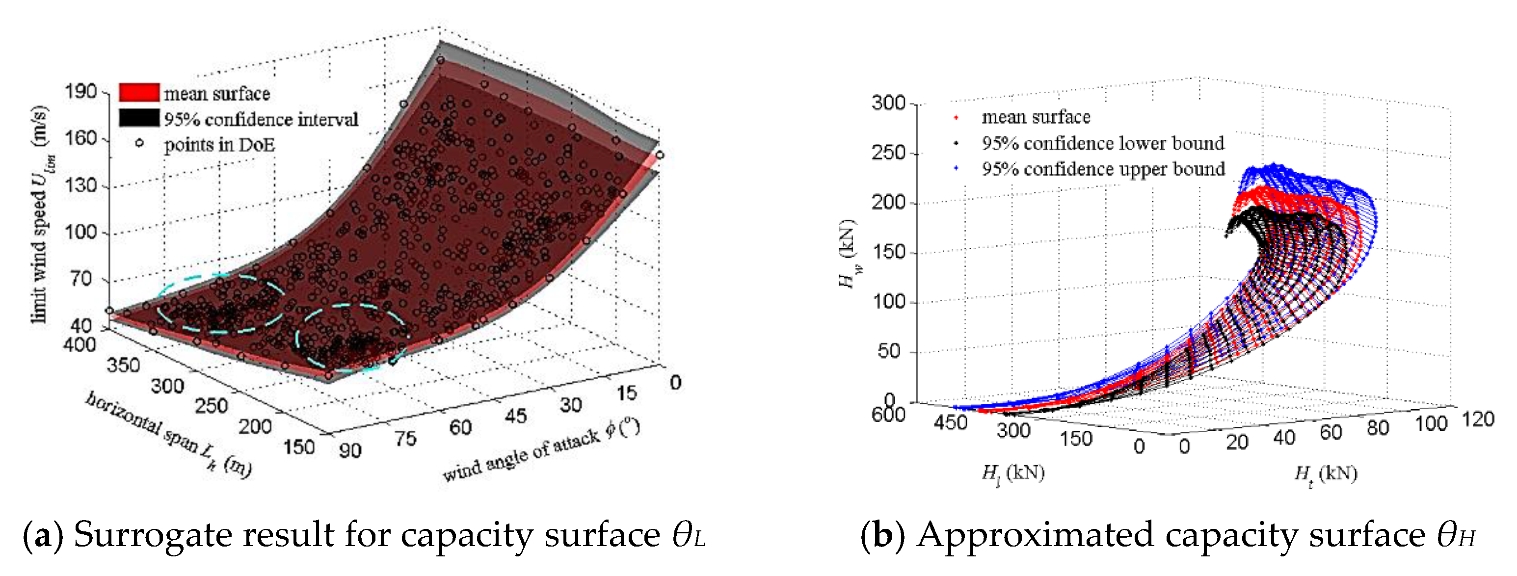
2.2.1. Capacity Surface
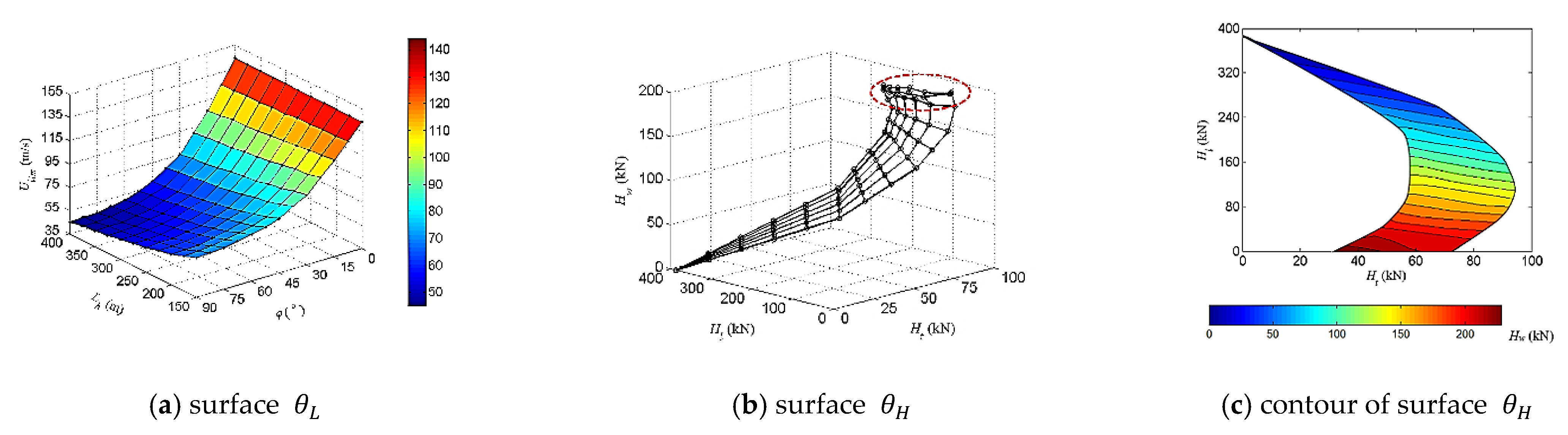
2.2.2. Example
2.2.3. Discussion
3. Kriging-Based Adaptive Surrogate Modeling for Limit Capacity of the Tower
3.1. Kriging Method
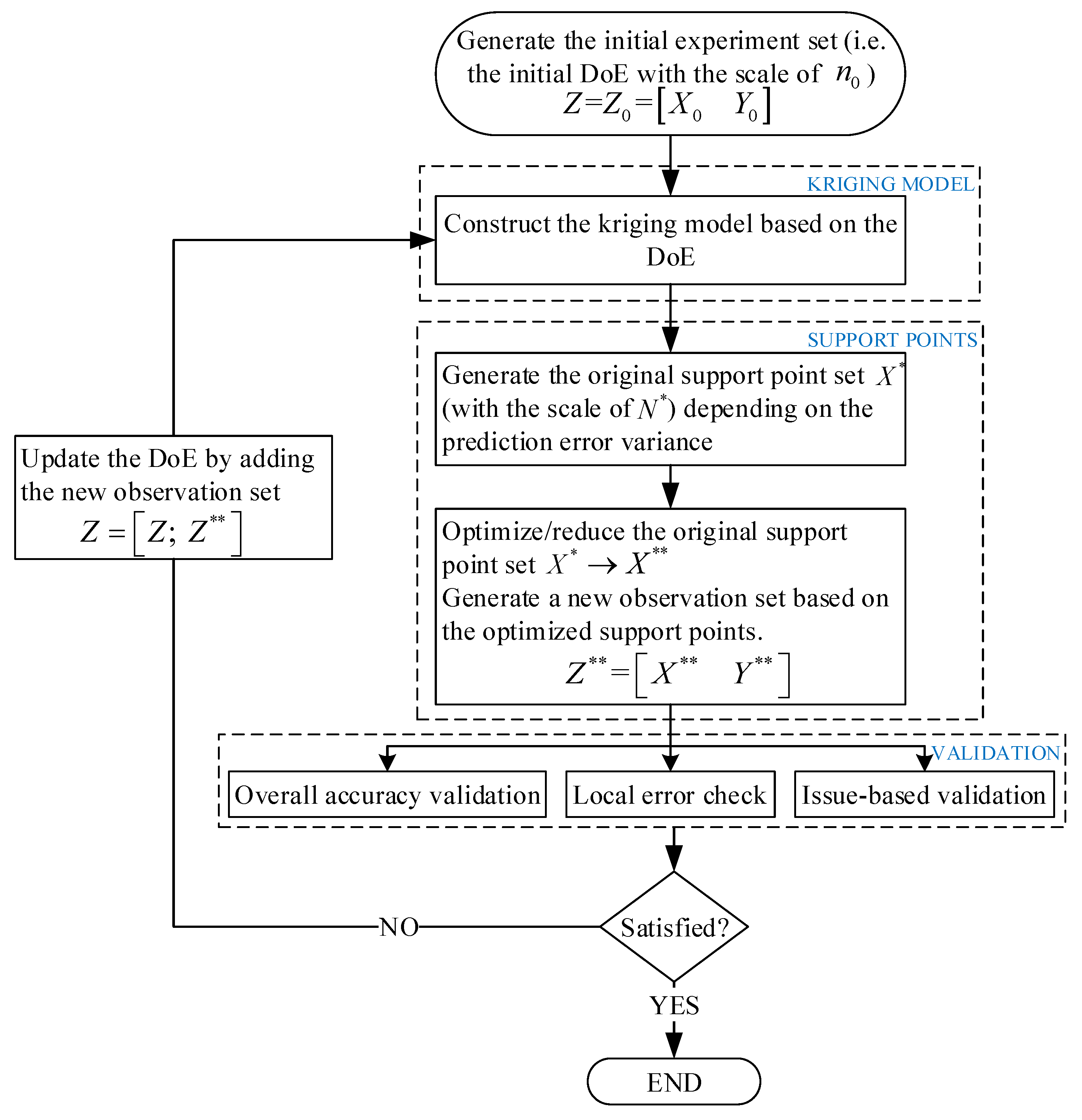
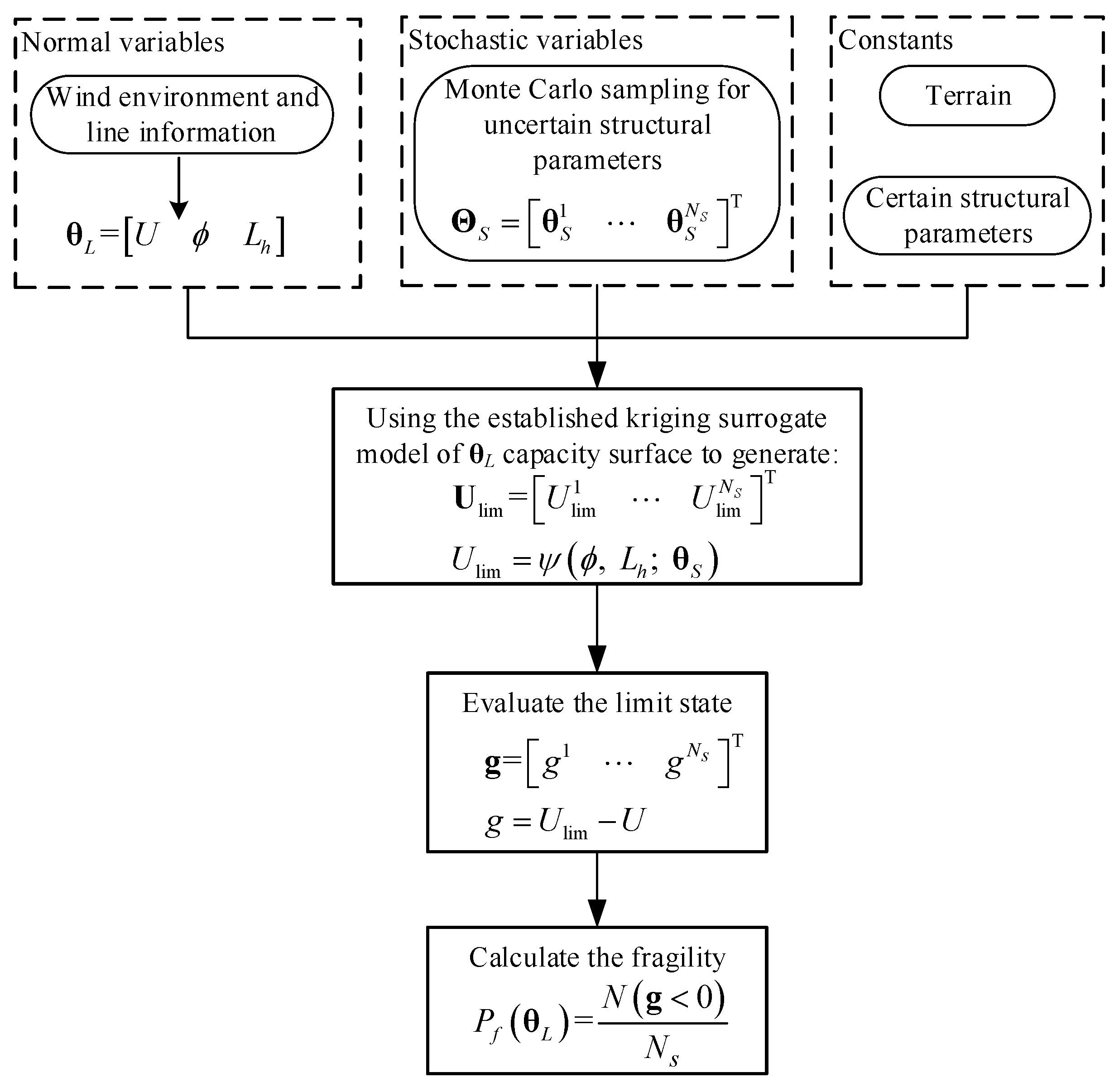
3.2. An Adaptive Modeling Framework
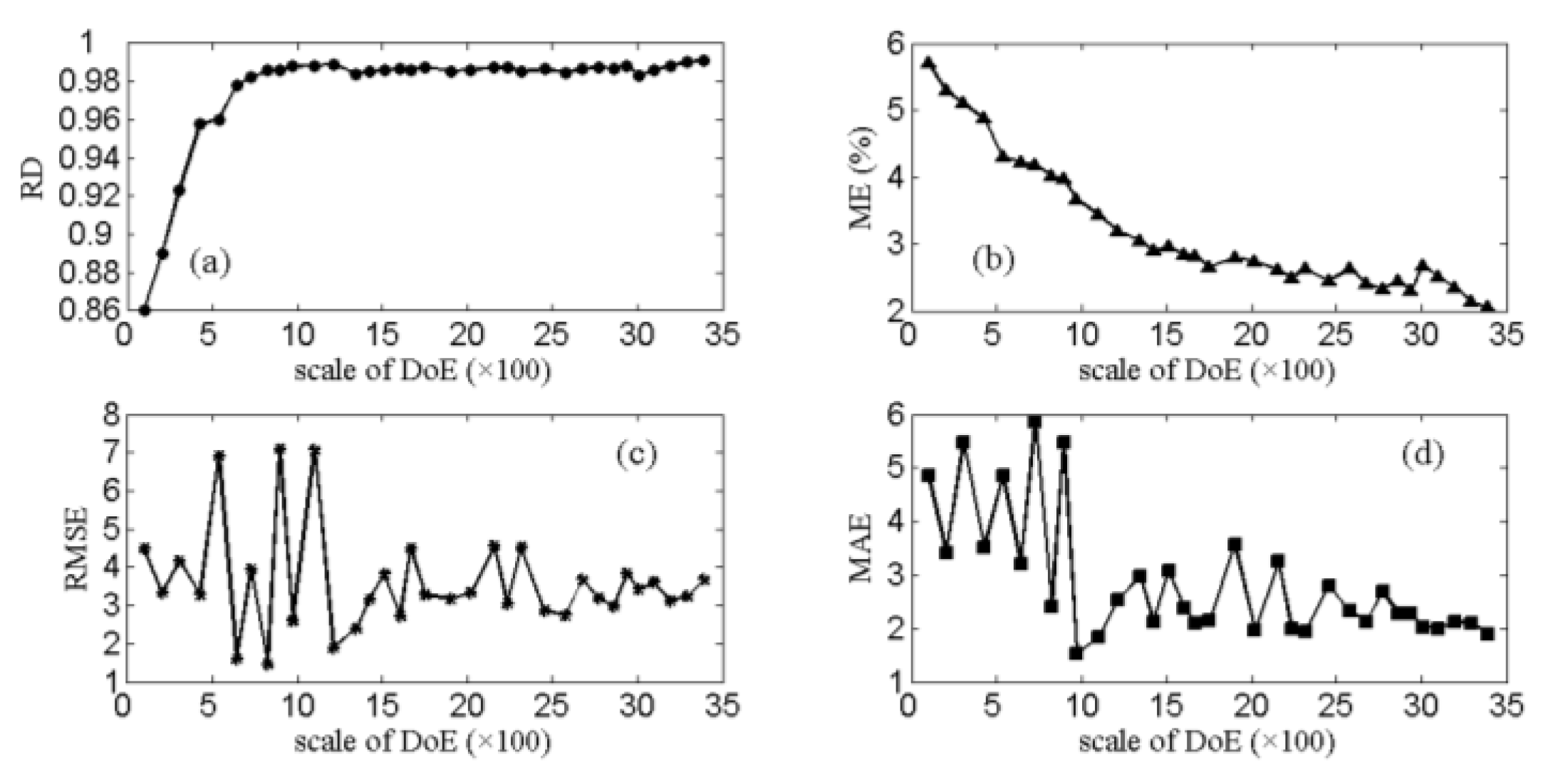
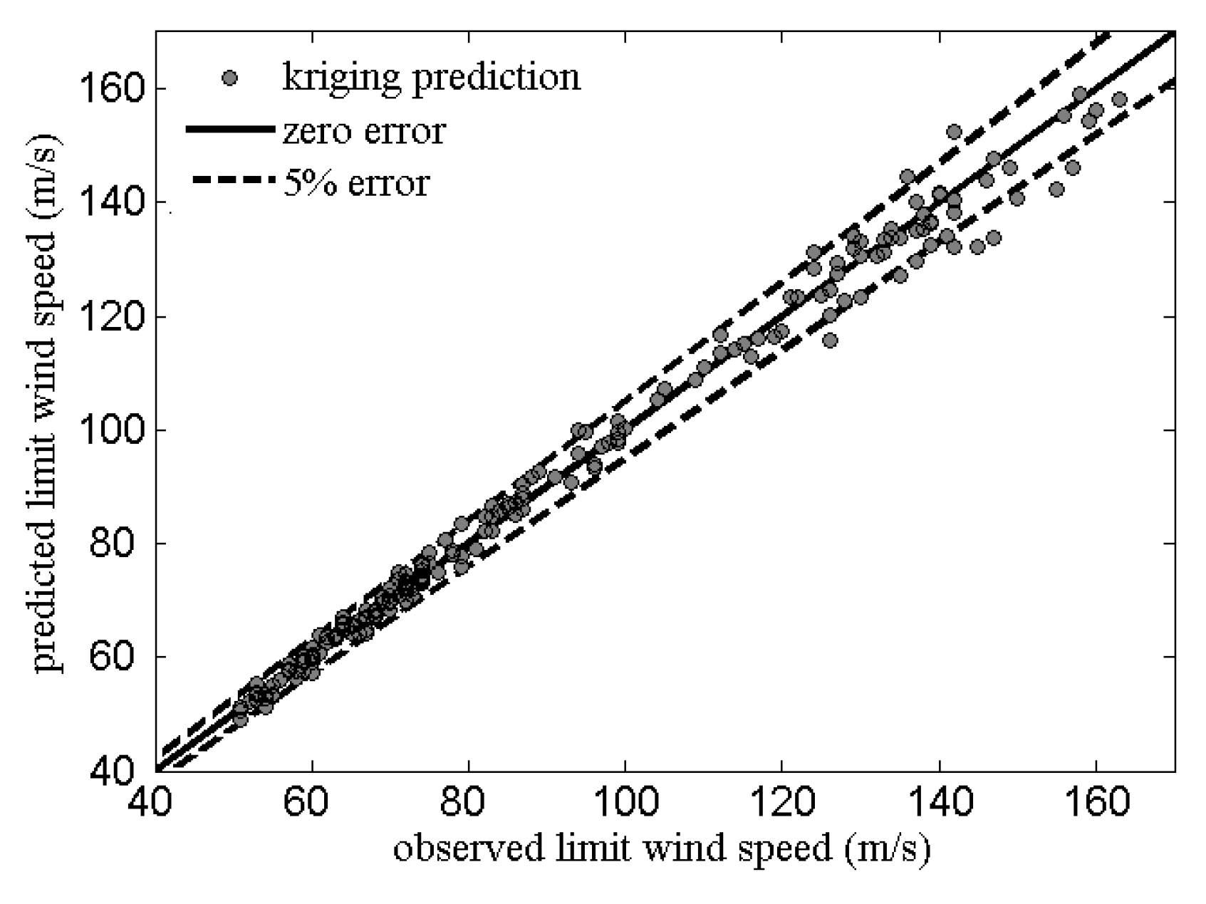
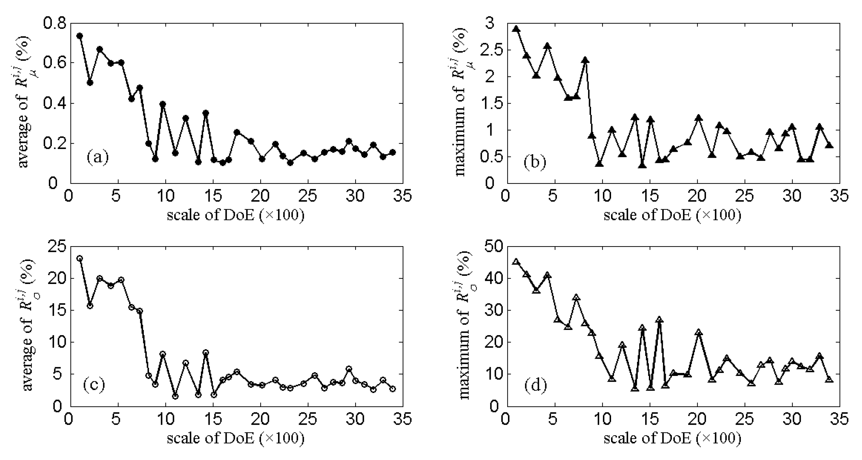
3.3. Example Study
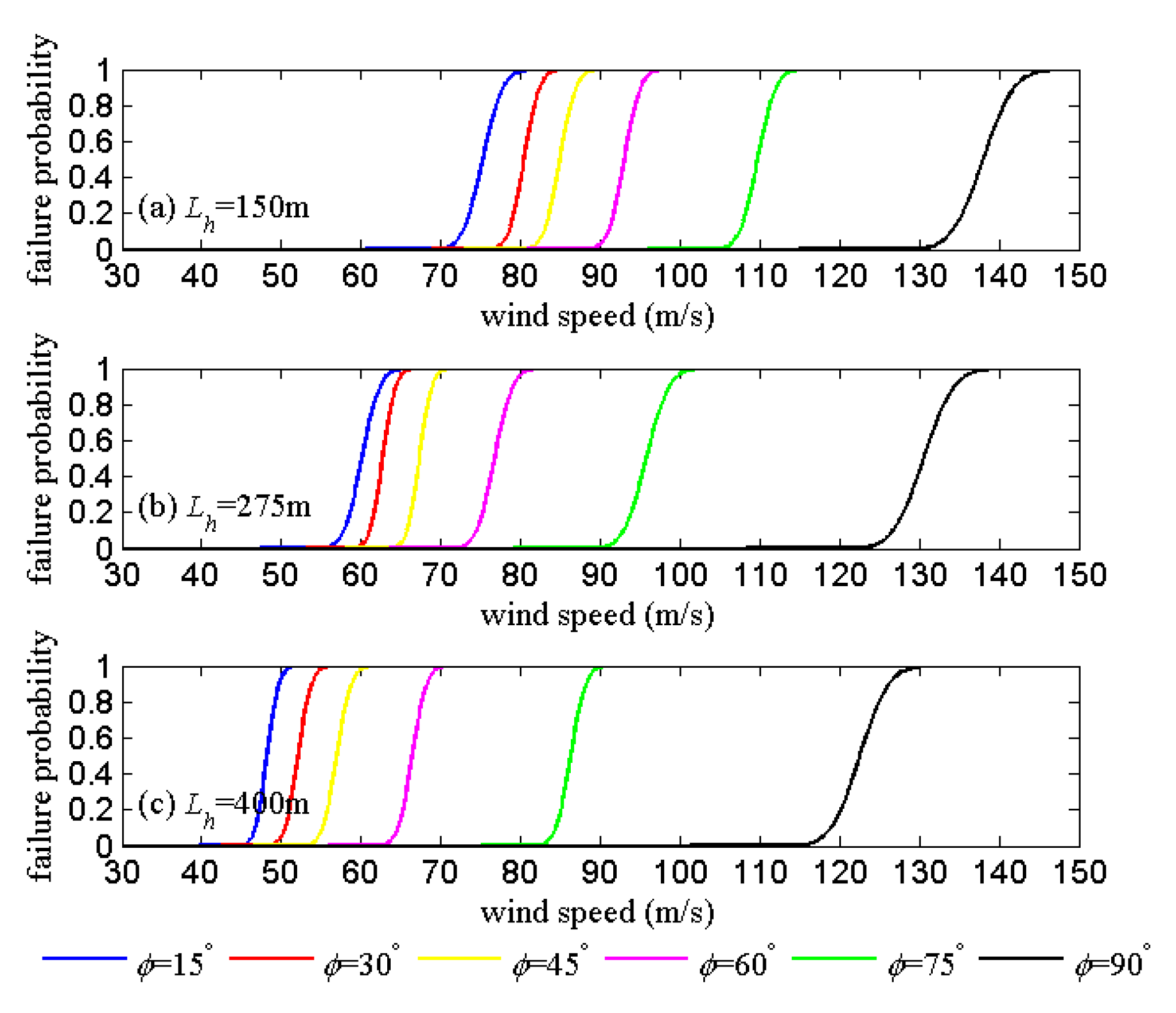
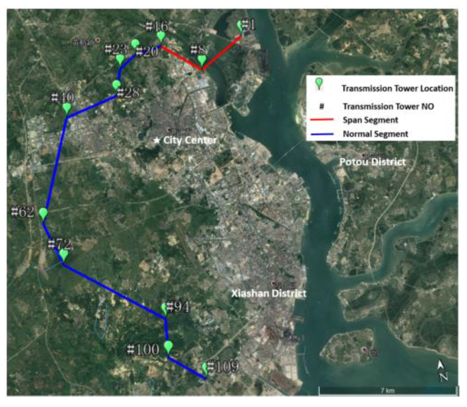
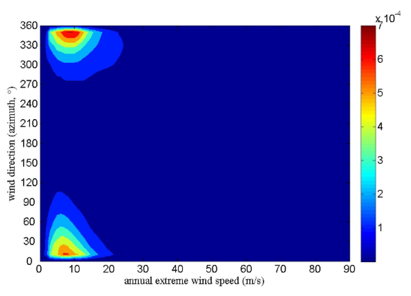
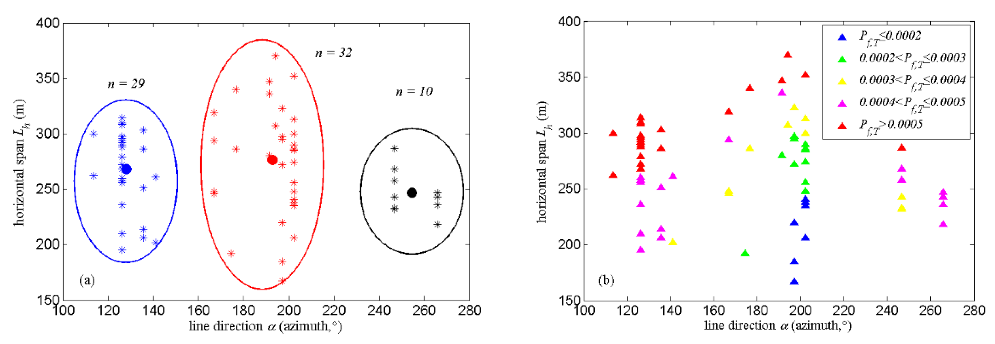
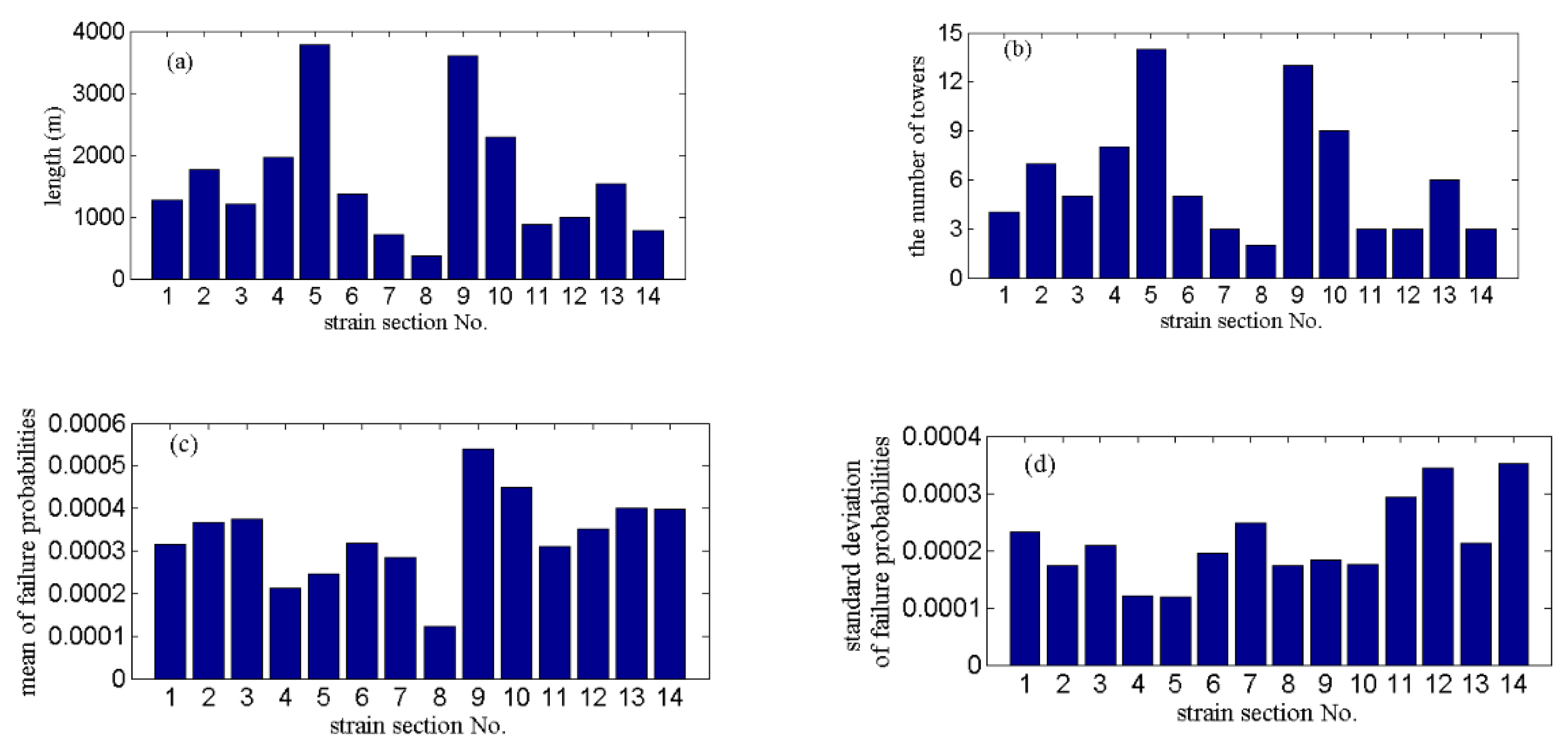
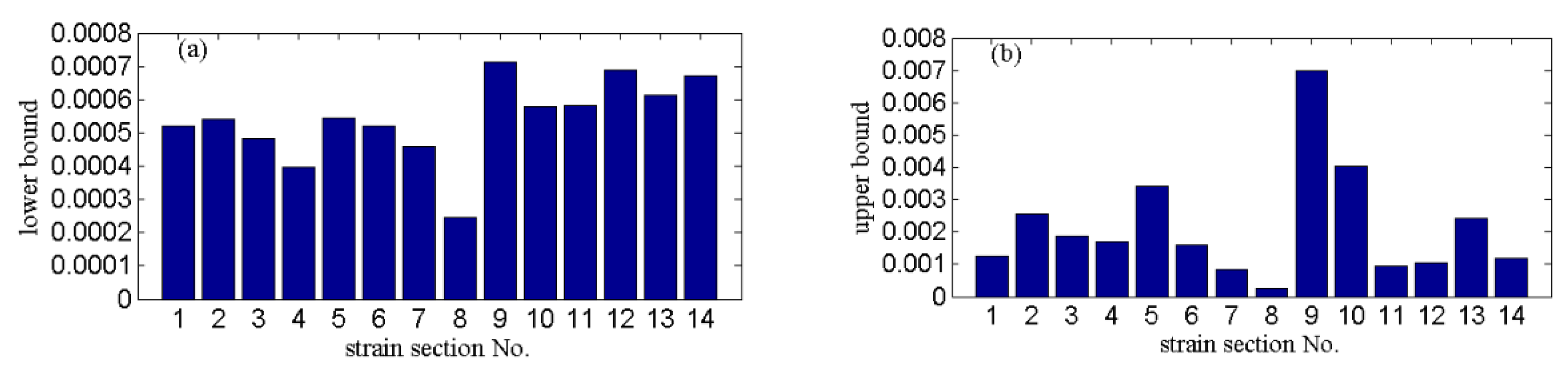
4. Application to the Structural Fragility Assessment on a Transmission Line
5. Conclusions
Author Contributions
Funding
Institutional Review Board Statement
Informed Consent Statement
Conflicts of Interest
Appendix A. Interaction between the Wind and the Transmission Line Towers

| Parameters | Tower Structure | Transmission Wires | Remarks |
|---|---|---|---|
| Combined wind factor [21] | The power law is adopted here. z is the height of concern, z0 is the reference height taken to be 10 m, and α0 is the roughness exponent. | ||
| Gust response factor [37] | Iz is the turbulence intensity of winds, B (including Bt and Bw) is the background component of the structural response, Ls is the integral scale of turbulence of winds, z is the height of the tower section, and S is the span of line. | ||
| Shape factor [38] | If d < 17 mm, μs,w = 1.2 If d ≥ 17 mm, μs,w = 1.1 | As and A are the projected area and the area of the outer profile of the tower section, respectively, η is the geometrical factor of the tower section, and d is the outer diameter of the wire. | |
| Span factor [39] | - | U < 20 m/s, α = 1.00; 20 m/s ≤ U < 27 m/s, α = 0.85; 27 m/s ≤ U < 31.5 m/s, α = 0.75; U ≥ 31.5 m/s, α = 0.70. | U is the 10-min-averaged wind speed at 10 m over the ground. |
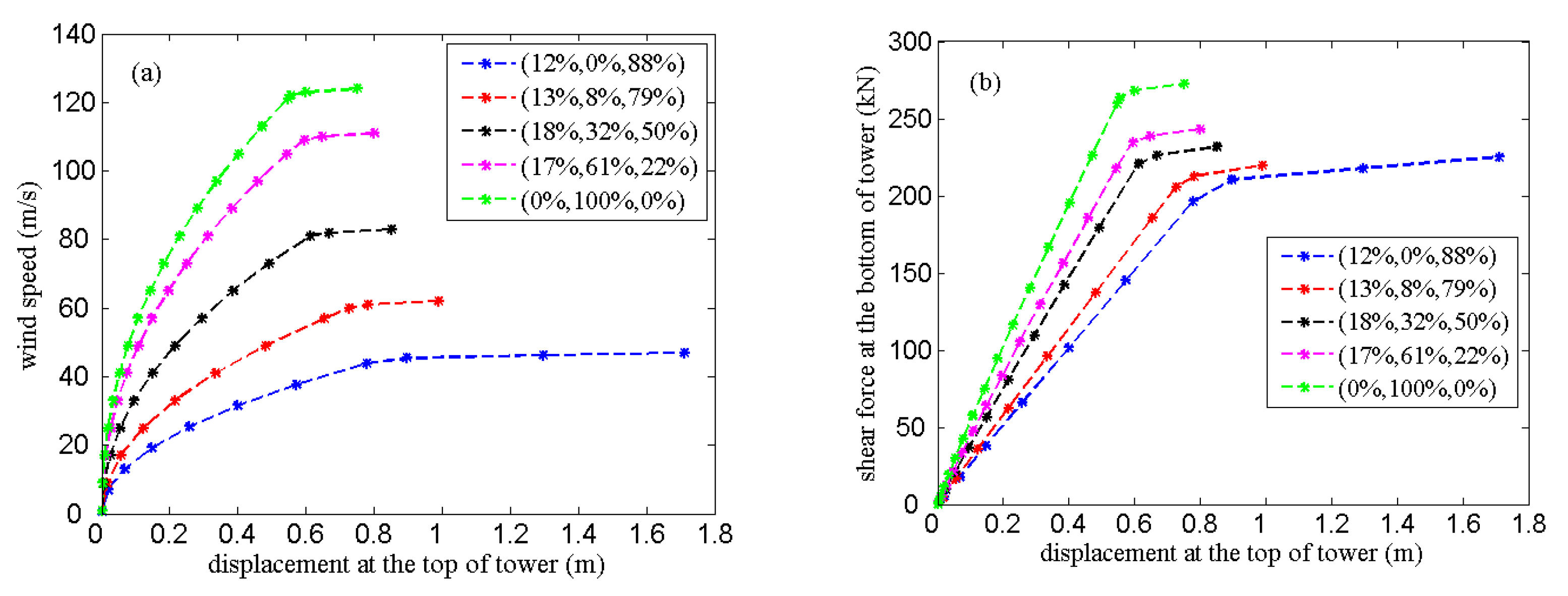
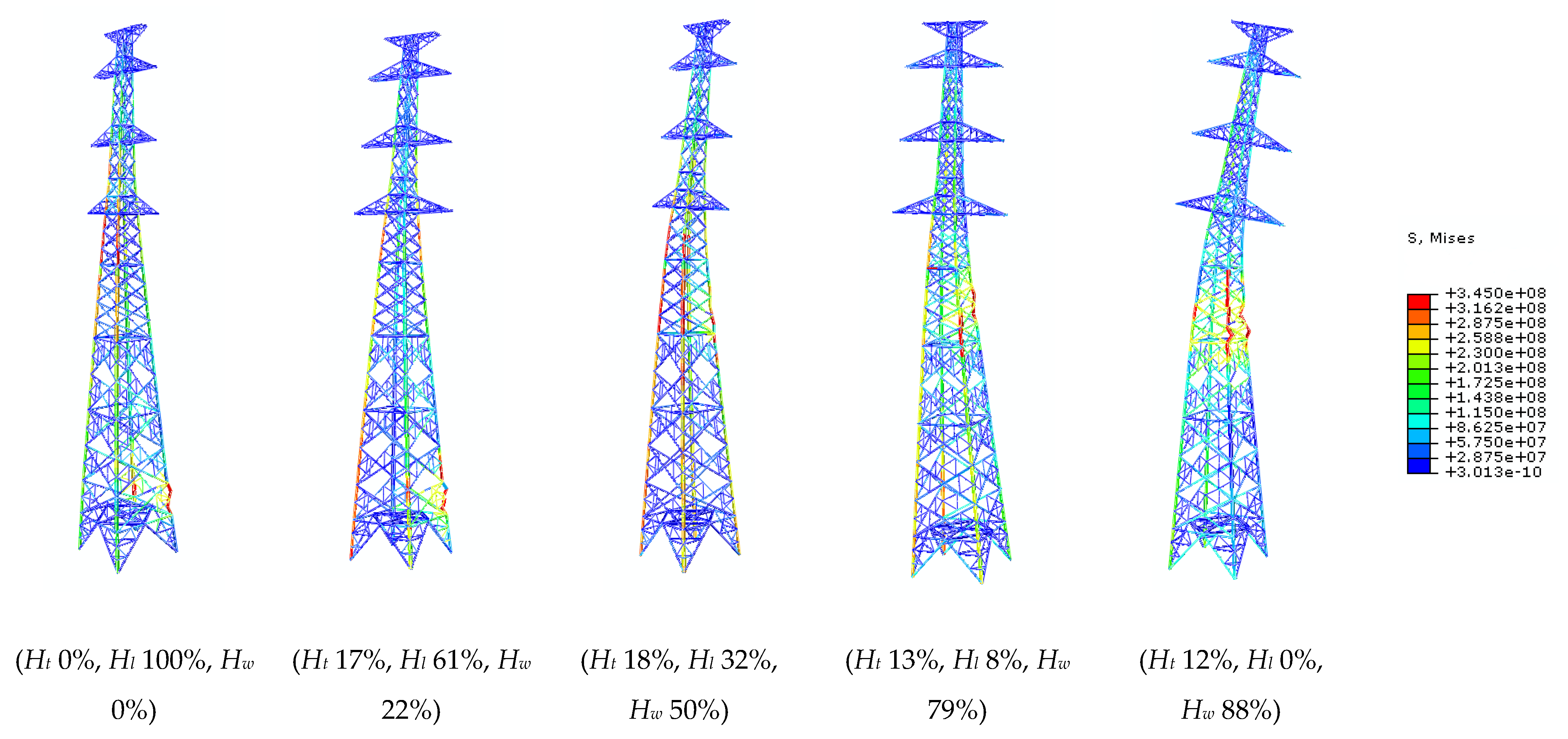
Appendix B. Simulation Results of the Limit Capacity of Transmission Towers under Winds


References
- Liu, Y.; Singh, C. Reliability evaluation of composite power systems using Markov cut-set method. IEEE Trans. Power Syst. 2010, 25, 777–785. [Google Scholar] [CrossRef]
- Vaiman, M.; Bell, K.; Chen, Y.; Chowdhury, B.; Dobson, I.; Hines, P.; Zhang, P. Risk assessment of cascading outages: Methodologies and challenges. IEEE Trans. Power Syst. 2012, 27, 631–641. [Google Scholar] [CrossRef]
- Panteli, M.; Mancarella, P. Influence of extreme weather and climate change on the resilience of power systems: Impacts and possible mitigation strategies. Elect. Power Syst. Res. 2015, 127, 259–270. [Google Scholar] [CrossRef]
- Panteli, M.; Pickering, C.; Wilkinson, S.; Dawson, R.; Mancarella, P. Power system resilience to extreme weather: Fragility modelling, probabilistic impact assessment, and adaptation measures. IEEE Trans. Power Syst. 2017, 32, 3747–3757. [Google Scholar] [CrossRef] [Green Version]
- Tao, T.; Shi, P.; Wang, H. Spectral modelling of typhoon winds considering nexus between longitudinal and lateral components. Renew. Energy 2020, 162, 2019–2030. [Google Scholar] [CrossRef]
- Tao, T.; Wang, H. Modelling of longitudinal evolutionary power spectral density of typhoon winds considering high-frequency subrange. J. Wind Eng. Ind. Aerod. 2019, 193, 103957. [Google Scholar] [CrossRef]
- Tao, T.; Shi, P.; Wang, H. Short-term prediction of downburst winds: A double-step modification enhanced approach. J. Wind Eng. Ind. Aerod. 2021, 211, 104561. [Google Scholar] [CrossRef]
- Alam, M.J.; Santhakumarj, A.R. System reliability analysis of transmission line towers. Comput. Struct. 1994, 53, 343–350. [Google Scholar] [CrossRef]
- Natarajan, K.; Santhakumar, A. Reliability-based optimization of transmission line towers. Comput. Struct. 1995, 55, 387–403. [Google Scholar] [CrossRef]
- Fenton, G.A.; Sutherland, N. Reliability-based transmission line design. IEEE Trans. Power Deliv. 2011, 26, 596–606. [Google Scholar] [CrossRef]
- Prasad, R.N.; Knight, G.M.S.; Mohan, S.J.; Lakshmanan, N. Studies on failure of transmission line towers in testing. Eng. Struct. 2012, 35, 55–70. [Google Scholar] [CrossRef]
- Qiang, X.; Li, S. Experimental study on the mechanical behavior and failure mechanism of a latticed steel transmission tower. J. Struct. Eng. 2013, 139, 1009–1018. [Google Scholar]
- Tapia-Hernández, E.; Ibarra-González, S.; De-León-Escobedo, D. Collapse mechanism of power towers under wind loading. Struct. Infrastruct. Eng. 2017, 13, 766–782. [Google Scholar] [CrossRef]
- Albermani, F.; Kitipornchai, S.; Chan, R.W.K. Failure analysis of transmission towers. Eng. Fail. Anal. 2009, 16, 1922–1928. [Google Scholar] [CrossRef]
- Yang, S.C.; Hong, H.P. Nonlinear inelastic responses of transmission tower-line system under downburst wind. Eng. Struct. 2016, 123, 490–500. [Google Scholar] [CrossRef]
- Fu, X.; Li, H.N.; Li, G. Fragility analysis and estimation of collapse status for transmission tower subjected to wind and rain loads. Struct. Safety 2016, 58, 1–10. [Google Scholar] [CrossRef]
- Fu, X.; Li, H.N. Uncertainty analysis of the strength capacity and failure path for a transmission tower under a wind load. J. Wind Eng. Ind. Aerod. 2018, 173, 147–155. [Google Scholar] [CrossRef]
- Fu, X.; Li, H.N.; Tian, L.; Wang, J.; Cheng, H. Fragility analysis of transmission line subjected to wind loading. J. Perform. Constr. Fac. 2019, 33, 04019044. [Google Scholar] [CrossRef]
- Cai, Y.Z.; Xie, Q.; Xue, S.T.; Hu, L.; Kareem, A. Fragility Modelling Framework for Transmission Line Towers under Winds. Eng. Struct. 2019, 191, 686–697. [Google Scholar] [CrossRef]
- DL/T 5154-2012. Technical Code for the Design of Tower and Pole Structures of Overhead Transmission Line (Industrial Standard); Electric Power Planning & Engineering Institute: Beijing, China, 2012. [Google Scholar]
- IEC 60826. Design Criteria of Overhead Transmission Lines, 3rd ed.; International Electro-technical Commission: Geneva, Switzerland, 2003. [Google Scholar]
- Mara, T.G.; Hong, H.P. Effect of wind direction on the response and capacity surface of a transmission tower. Eng. Struct. 2013, 57, 493–501. [Google Scholar] [CrossRef]
- Sacks, J.; Welch, W.J.; Mitchell, T.J.; Wynn, H.P. Design and analysis of computer experiments. Stat. Sci. 1989, 4, 409–435. [Google Scholar] [CrossRef]
- Dubourg, V.; Sudret, B.; Bourinet, J.M. Reliability-based design optimization using kriging surrogates and subset simulation. Struct. Multidisc. Optim. 2011, 44, 673–690. [Google Scholar] [CrossRef] [Green Version]
- Irfan, K. Application of kriging method to structural reliability problems. Struct. Safety 2005, 27, 133–151. [Google Scholar]
- Ioannis, G.; Alexandros, A.T.; George, P.M. Kriging metamodeling in seismic risk assessment based on stochastic ground motion models. Earthq. Eng. Struct. Dyn. 2015, 44, 2377–2399. [Google Scholar]
- Robert, C.P.; Casella, G. Monbte Carlo Statistical Methods, 2nd ed.; Springer: New York, NY, USA, 2004. [Google Scholar]
- Hartigan, J.A.; Wong, M.A. Algorithm AS 136: A K-means clustering algorithm. J. R. Stat. Soc. C 1979, 28, 100–108. [Google Scholar] [CrossRef]
- Kovaleva, E.V.; Mirkin, B.G. Bisecting k-means and 1D projection divisive clustering: A unified framework and experimental comparison. J. Classif. 2015, 32, 414–442. [Google Scholar] [CrossRef]
- Meckesheimer, M.; Booker, A.J.; Barton, R.R.; Simpson, T.W. Computationally inexpensive metamodel assessment strategies. AIAA J. 2002, 40, 2053–2060. [Google Scholar] [CrossRef]
- Takeuchi, M.; Maeda, J.; Ishida, N. Aerodynamic damping properties of two transmission towers estimated by combining several identification methods. J. Wind Eng. Ind. Aerod. 2010, 98, 872–880. [Google Scholar] [CrossRef]
- JCSS. Probabilistic Model Code–Part 3-Material Properties. JCSS. 2001. Available online: https://www.jcss-lc.org/jcss-probabilistic-model-code/ (accessed on 1 January 2021).
- Google Earth Pro V7.3.3.7786. Zhanjiang, Guangzhou Province, China. 21°16′13″ N 110°21′33″ E, Eye alt 45 km. Available online: https://www.google.com/earth/ (accessed on 10 September 2017).
- Ying, M.; Zhang, W.; Yu, H.; Lu, X.; Feng, J.; Fan, Y.; Zhu, Y.; Chen, D. An overview of the China Meteorological Administration tropical cyclone database. J. Atmos. Ocean Technol. 2014, 31, 287–301. [Google Scholar] [CrossRef] [Green Version]
- Lu, X.Q.; Yu, H.; Yang, X.M.; Li, X.F. Estimating Tropical Cyclone Size in the Northwestern Pacific from Geostationary Satellite Infrared Images. Remote Sens. 2017, 9, 728. [Google Scholar] [CrossRef] [Green Version]
- Cai, Y.Z. Typhoon Fragility for Electric Transmission Line Based on the Failure of Transmission Towers. Ph.D. Thesis, Tongji University, Shanghai, China, 2019. [Google Scholar]
- Bowman, A.W.; Azzalini, A. Applied Smoothing Techniques for Data Analysis; Oxford University Press: New York, NY, USA, 1997. [Google Scholar]
- ASCE. Guidelines for Electrical Transmission Line Structural Loading, 3rd ed.; ASCE Manuals and Reports on Engineering Practice No. 74; ASCE: Reston, VA, USA, 2010. [Google Scholar]
- GB 50009-2012. Load Code for the Design of Building Structures (National Standard); Ministry of Construction of the People’s Republic of China: Beijing, China, 2012.
- GB 50545-2010. Code for Design of 110 kV~750 kV Overhead Transmission Line (National Standard); China Electricity Council: Beijing, China, 2010. [Google Scholar]


| Tower ZY | |
|---|---|
| Type | Double-Circuit Angle-Steel Lattice Suspension Tower |
| Total height (m) | 45.5 |
| Body height (m) | 30 |
| Steel type | Q345, Q235 [14] |
| Foot distance (m) | 6.4 |
| Natural frequency (Hz) | 2.037 (transverse), 2.047 (longitudinal) |
| Damping ratio | 0.01 |
| Transmission wires (conductors and ground wires) | |
| Type | LGJQ-300/40 (two-bundle conductors) LGJQ-95/55 (ground wires) |
| Linear density (kg/m) | 2.2660 (conductors), 0.7077 (ground wires) |
| Effective diameters (mm) | 47.88 (conductors), 16 (ground wires) |
| Transmission line | |
| Horizontal span (m) | maximum 370/minimum 127/average 275 |
| Direction (azimuth, °) | maximum 265.82/minimum 113.49/average 181.08 |
| Terrain | Open (C exposure) |
| Material [32] | Mean (μ) | C.O.V (δ) | Distribution |
|---|---|---|---|
| Yield strength (fy,Q345) | 387 MPa | 0.07 | Lognormal |
| Yield strength (fy,Q235) | 264 MPa | 0.07 | Lognormal |
| Elastic modulus (Es) | 206,000 MPa | 0.03 | Lognormal |
| Poisson ratio (ν) | 0.3 | 0.03 | Lognormal |
| Geometry [17] | Mean */standard deviation (μ/σ) | C.O.V (δ) | Distribution |
| Thickness of angle steel members (t) | 0.985 | 0.032 | Normal |
| Length of angle steel members (l) | 1.001 | 0.008 | Normal |
Publisher’s Note: MDPI stays neutral with regard to jurisdictional claims in published maps and institutional affiliations. |
© 2021 by the authors. Licensee MDPI, Basel, Switzerland. This article is an open access article distributed under the terms and conditions of the Creative Commons Attribution (CC BY) license (https://creativecommons.org/licenses/by/4.0/).
Share and Cite
Cai, Y.; Wan, J. Wind-Resistant Capacity Modeling for Electric Transmission Line Towers Using Kriging Surrogates and Its Application to Structural Fragility. Appl. Sci. 2021, 11, 4714. https://0-doi-org.brum.beds.ac.uk/10.3390/app11114714
Cai Y, Wan J. Wind-Resistant Capacity Modeling for Electric Transmission Line Towers Using Kriging Surrogates and Its Application to Structural Fragility. Applied Sciences. 2021; 11(11):4714. https://0-doi-org.brum.beds.ac.uk/10.3390/app11114714
Chicago/Turabian StyleCai, Yunzhu, and Jiawei Wan. 2021. "Wind-Resistant Capacity Modeling for Electric Transmission Line Towers Using Kriging Surrogates and Its Application to Structural Fragility" Applied Sciences 11, no. 11: 4714. https://0-doi-org.brum.beds.ac.uk/10.3390/app11114714