Laminar-Turbulent Transition Localization in Thermographic Flow Visualization by Means of Principal Component Analysis

Featured Application

The thermographic flow visualization in applications with low thermal contrast is directly applicable for in-process measurements on wind turbines in operation to analyze, non-invasively and without contact, the boundary layer flow on rotor blades.

Abstract

Thermographic flow visualization is a contactless, non-invasive technique to visualize the boundary layer flow on wind turbine rotor blades, to assess the aerodynamic condition and consequently the efficiency of the entire wind turbine. In applications on wind turbines in operation, the distinguishability between the laminar and turbulent flow regime cannot be easily increased artificially and solely depends on the energy input from the sun. State-of-the-art image processing methods are able to increase the contrast slightly but are not able to reduce systematic gradients in the image or need excessive a priori knowledge. In order to cope with a low-contrast measurement condition and to increase the distinguishability between the flow regimes, an enhanced image processing by means of the feature extraction method, principal component analysis, is introduced. The image processing is applied to an image series of thermographic flow visualizations of a steady flow situation in a wind tunnel experiment on a cylinder and DU96W180 airfoil measurement object without artificially increasing the thermal contrast between the flow regimes. The resulting feature images, based on the temporal temperature fluctuations in the images, are evaluated with regard to the global distinguishability between the laminar and turbulent flow regime as well as the achievable measurement error of an automatic localization of the local flow transition between the flow regimes. By applying the principal component analysis, systematic temperature gradients within the flow regimes as well as image artefacts such as reflections are reduced, leading to an increased contrast-to-noise ratio by a factor of 7.5. Additionally, the gradient between the laminar and turbulent flow regime is increased, leading to a minimal measurement error of the laminar-turbulent transition localization. The systematic error was reduced by 4% and the random error by 5.3% of the chord length. As a result, the principal component analysis is proven to be a valuable complementary tool to the classical image processing method in flow visualizations. After noise-reducing methods such as the temporal averaging and subsequent assessment of the spatial expansion of the boundary layer flow surface, the PCA is able to increase the laminar-turbulent flow regime distinguishability and reduce the systematic and random error of the flow transition localization in applications where no artificial increase in the contrast is possible. The enhancement of contrast increases the independence from the amount of solar energy input required for a flow evaluation, and the reduced errors of the flow transition localization enables a more precise assessment of the aerodynamic condition of the rotor blade.

1. Introduction

Flow visualization on wind turbines in operation enables an evaluation of the actual aerodynamic condition of a rotor blade. In particular, the position of the boundary layer flow transition between laminar and turbulent is of interest for the efficiency of the wind turbine because it correlates directly with the lift and drag of the airfoil [1].

One possibility of visualizing the boundary layer flow on an airfoil is given by the thermographic flow visualization that makes use of the relation between the heat transfer coefficient and the local skin friction between the fluid and the surface [2]. The technique is an already long established method in wind tunnel experiments to visualize the boundary layer flow [3,4,5] and enables the analysis of the laminar-turbulent flow transition [6,7], the laminar separation bubble [8,9] and turbulent separation [10]. For wind turbines in operation, the thermographic flow visualization is particularly suitable because it is a non-invasive, contactless approach without the need for surface preparation [11]. In addition to the required infrared camera located on the ground in a distance of 100 $\mathrm{m}$ to 300 $\mathrm{m}$, image processing is essential to enable a thermographic flow analysis. The image processing is needed to automatically extract the image information that provides a flow visualization with a high distinguishability between the different flow regimes and that finally enables the localization of the laminar-turbulent flow transition with a minimal measurement error.

Influencing factors reducing the global distinguishability between different flow regimes in thermographic flow visualizations exist as a result of the flow characteristics and external interference. Flow characteristics cause systematic temperature gradients within a flow regime region due to a non-constant heat flux as well as random temperature fluctuations due to flow fluctuations. External interferences are systematic temperature gradients due to reflections and random measurement noise. To cope with the effects of these influencing factors, the distinguishability between different flow regimes is usually maximized by increasing the initial temperature difference between fluid and surface with an active heating or cooling [5,6,7,12,13], respectively, while the influence of reflections is further minimized by subtracting a reference image that was acquired by prior measurements with no flow [7]. Since the temperature difference between fluid and surface cannot be altered in free-field applications on wind turbines in operation without excessive effort, and reference images cannot be acquired, an image processing of the raw thermographic images is desired that is able to cope with the effects of the influence factors and maximizes the flow regimes’ distinguishability.

Classical image processing methods for the thermographic flow visualization automatically result in a single output image. For instance, the averaging of a series of thermographic images of a steady flow situation leads to a minimized measurement noise and thus increases the signal-to-noise ratio. Crawford et al. [14] introduced an automatic evaluation with a spatial low-pass filter to increase the signal-to-noise ratio in single images of in-flight experiments. Both methods increase the distinguishability between flow regimes by minimizing the random image inhomogeneity. However, systematic influences remain present. Another image processing introduced by Dollinger et al. [15] focuses on temperature fluctuations and evaluates the temporal standard deviation of an image series to increase the distinguishability between flow regimes by reducing random and systematic inhomogeneities. These classical methods enable a straightforward, reproducible image processing, but systematic image inhomogeneities are either not or only partially corrected, which still limits the flow regimes’ distinguishability.

Other studies focus on enhanced image processing methods that extract the desired information from a thermographic image series. Dollinger et al. [15] applied a Fourier analysis by means of a discrete Fourier transform for each pixel over the image series and selected a certain frequency range to evaluate the mean amplitude of the temporal fluctuations. The evaluation of temporal fluctuations around the mean temperature is unaffected by systematic spatial inhomogeneities within the flow regimes and therefore has the potential to increase the distinguishability between the flow regimes. However, in order to maximize the distinguishability, a priori knowledge about the frequency range of the characteristic temperature fluctuations is needed. Another evaluation of temperature fluctuations without the assumption of a harmonic basis was recently tested by means of a Non-Negative Matrix Factorization [16]. The algorithm evaluates temporal and spatial image information in order to separate superimposed influences on the thermographic image series, leading to a flow visualization result with decreased random and systematic inhomogeneities and, thus, an increased distinguishability between the flow regimes. However, the non-reproducibility of the output images necessitates a manual post-processing as well as a priori knowledge about the approximate location of the flow regimes in order to identify the optimal output image. An enhanced image processing method that also evaluates spatial and temporal image information, without the assumption of a harmonic base, but provides reproducible results, is the principal component analysis (PCA). PCA is already a standard method for thermographic structure analysis [17], but its potential for the thermographic flow analysis has not yet been studied. Furthermore, the combination of classical and enhanced image processing methods seems promising to maximize the flow regimes’ distinguishability, which is a pending research task.

An important subsequent measurement task based on the flow visualization result is the localization of the laminar-turbulent flow transition. In order to achieve this, different image processing methods have been proposed. The most frequently applied approach is to use either unprocessed raw images or the output of a simple image filtering such as averaging, and then to locate the maximum temperature gradient along the temperature profiles in the main flow direction [12,18,19,20]. For a dynamically changing boundary layer flow, Wolf et al. [21] used the computation of differential images to visualize the laminar-turbulent flow transition on a fast pitching airfoil. Crawford et al. [14] introduced an automatic localization of the laminar-turbulent flow transition by means of a spatial low-pass filter and a subsequent edge detection algorithm. However, the achievable measurement uncertainty for the localization of the laminar-turbulent flow transition was first investigated by Dollinger et al. 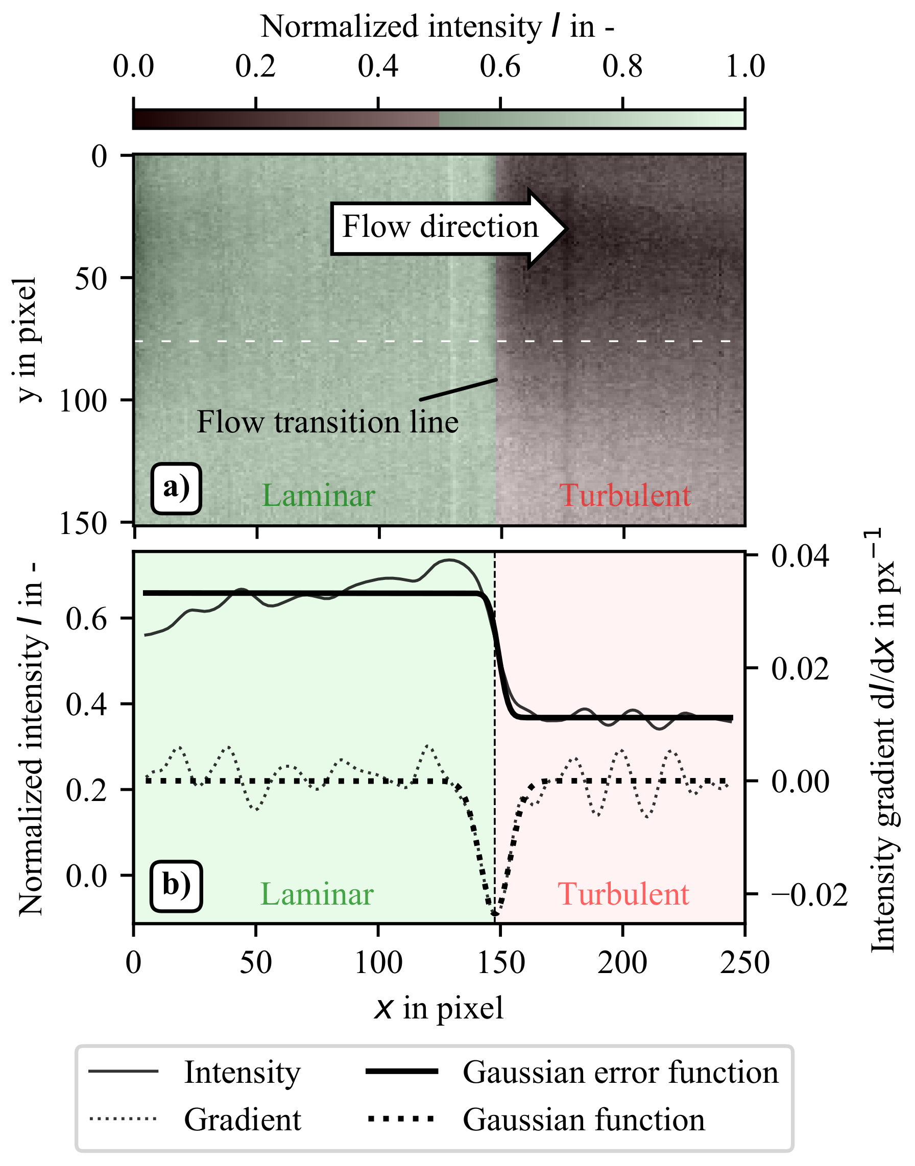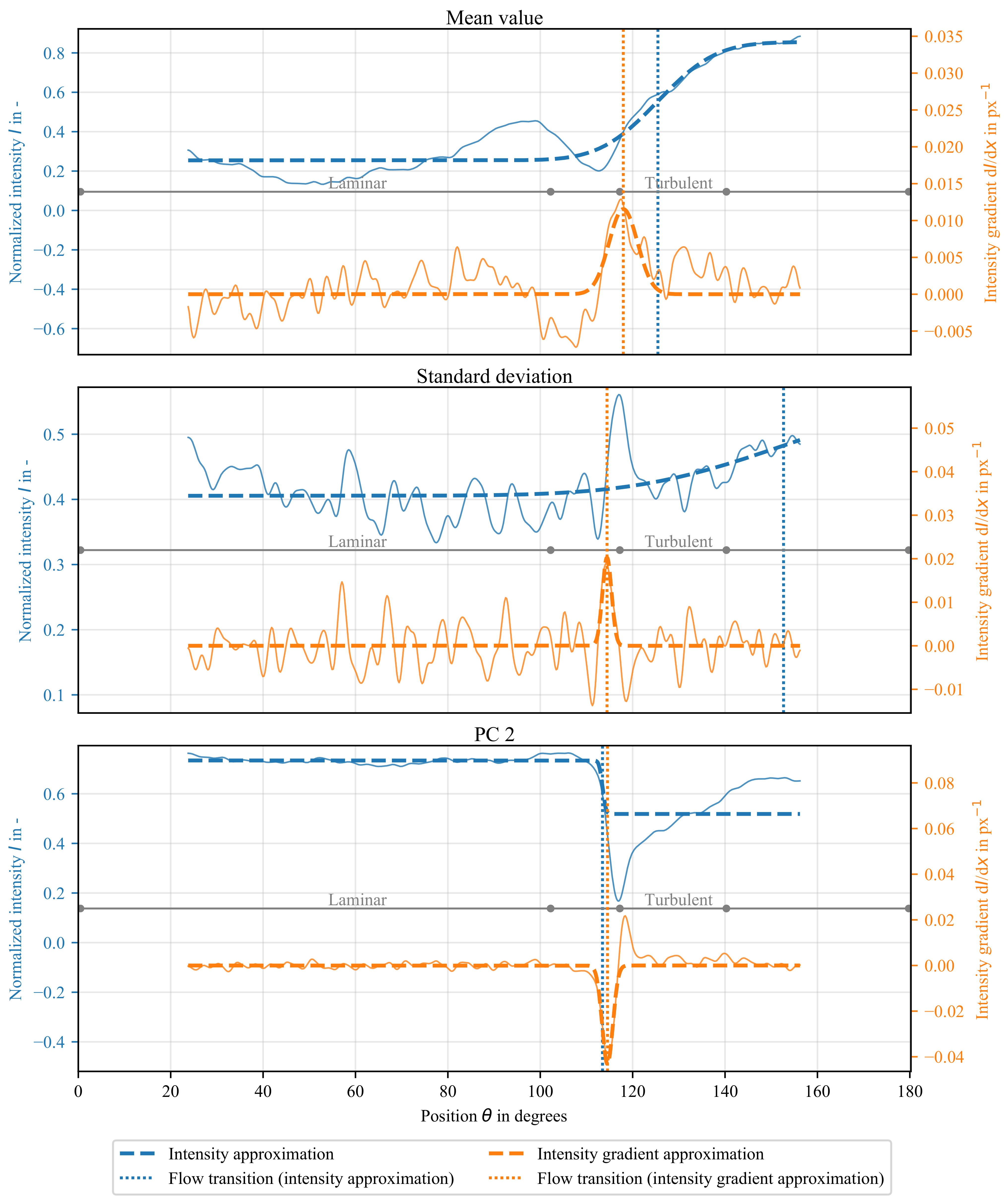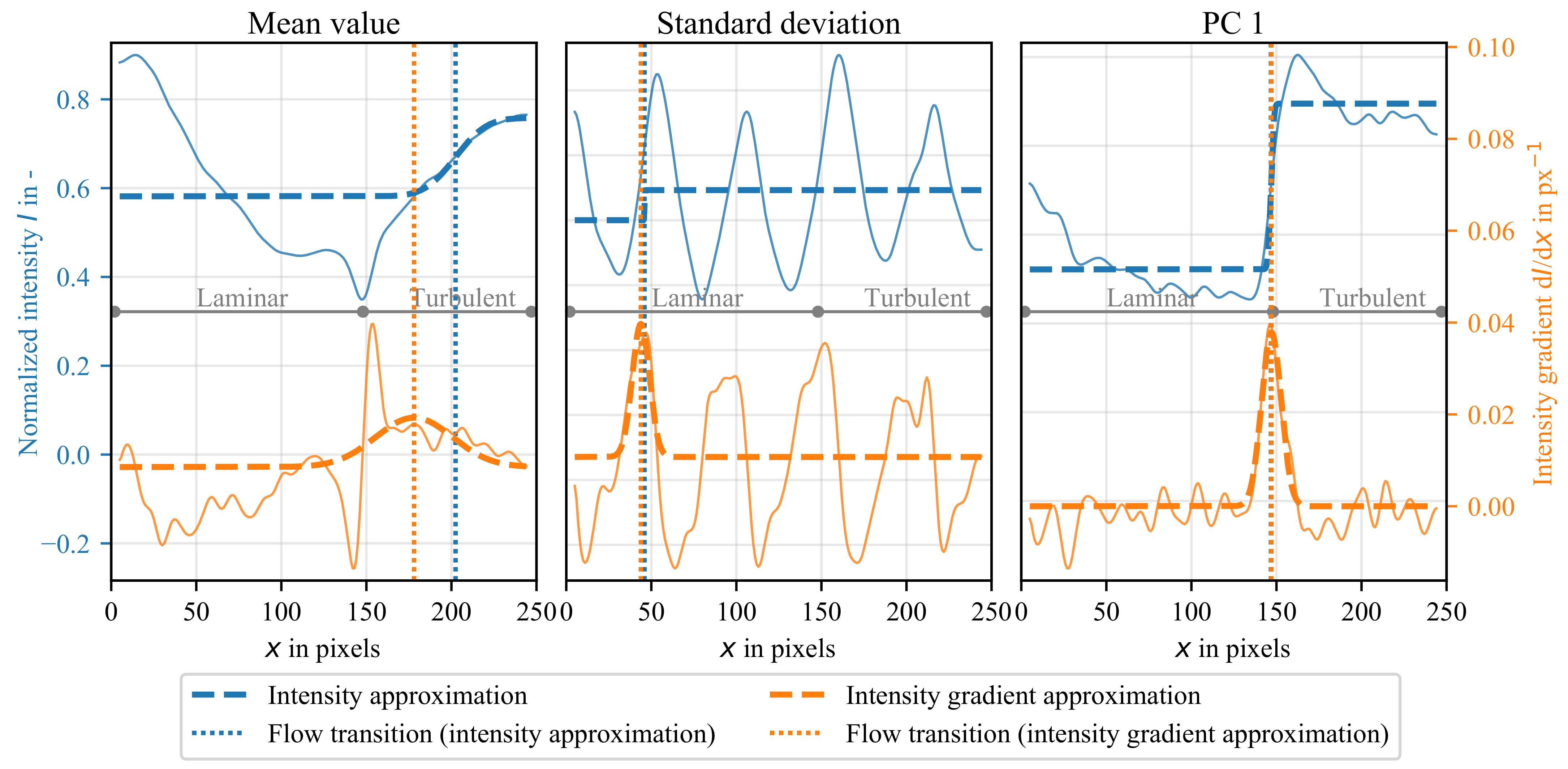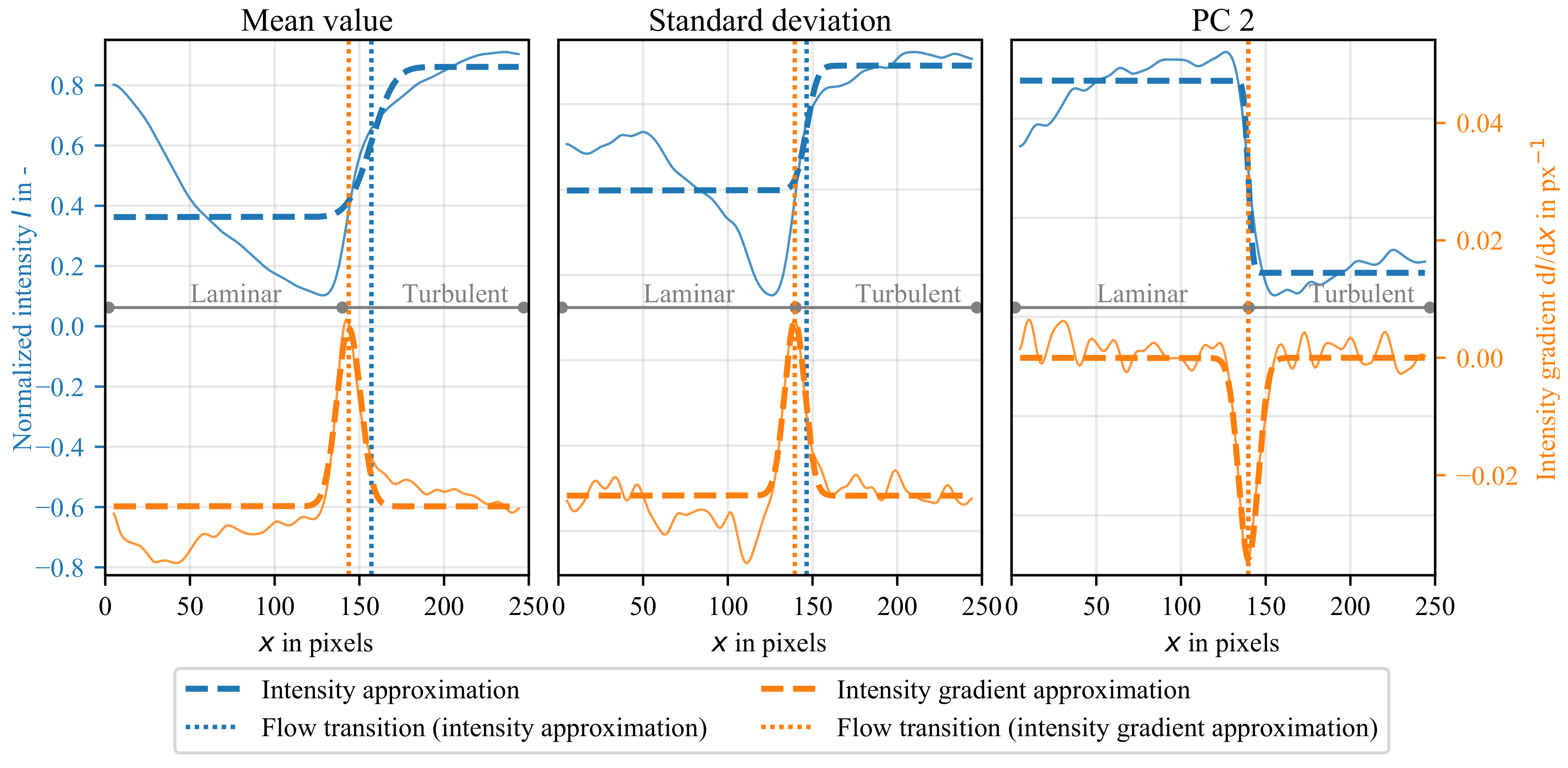[22] in unprocessed thermographic raw images. According to their findings, the uncertainty is inversely proportional to the temperature gradient between the laminar and turbulent flow regime. Additionally, it was shown that the ideal localization method for locating the flow transition with a minimal uncertainty and a sub-pixel accuracy is to apply a least-squares approximation of the temperature profile with a Gaussian error function. As an alternative, the gradient of the temperature profile can be approximated by a Gaussian function. If the temperature profile or its gradient has the expected course according to the respective approximation, the flow transition position can be extracted directly by the parameters of the fitted approximation function. However, since the ideal temperature course is disturbed by different naturally occurring systematic and random influences, enhanced image processing that reduces these influences has the potential to improve the flow transition localization. The thermographic flow visualization with enhanced image processing methods was, however, not yet investigated with regard to the position error of the laminar-turbulent flow transition.

Therefore, the present article focuses on an enhanced image processing for thermographic flow visualization by means of a PCA to maximize the distinguishability between the laminar and turbulent flow regime and to minimize interferences. The resulting flow visualization is further assessed concerning the achievable measurement error of the flow transition localization. Furthermore, the combination of the PCA with classical image processing methods is studied to extract the maximal laminar-turbulent flow information from thermographic image series.

Section 2 introduces the PCA and the figure of merit to evaluate the contrast between the visualized flow regimes and explains the flow transition localization by means of an approximation with a Gaussian error function or a Gaussian function. Section 3 describes the thermographic experimental setup of the wind tunnel experiments. The image processing results of the experimental data are studied with respect to the maximized contrast in the flow visualization as well as the error of the flow transition localization in Section 4. The article finishes with a summary and outlook in Section 5.

2. Measurement Approach

At first, the following section introduces the PCA as a feature extraction method and explains the hypothesis of its capability to create flow visualizations with increased distinguishability between the laminar and turbulent flow regimes. Afterwards, the quantification of the distinguishability between flow regimes by means of the contrast-to-noise ratio is presented. Lastly, the signal processing for localizing the laminar-turbulent flow transition is introduced.

2.1. Principal Component Analysis (PCA)

PCA [23] is a multivariate statistical procedure with the goal of extracting the important information of a dataset and representing them as uncorrelated variables, called principal components (PCs) [24]. The PCs are characterized by their orthogonal orientation to each other and are sorted according to their variance. Therefore, the first PC inherits the most distinct information of the data set, hence representing the highest variety of the complete data set. As a result, the first N PC can be linearly combined to approximate each individual input of the data set sufficiently, while N remains much lower than the number of individual input data. This can be interpreted as a dimensionality reduction while most of the information to distinguish between the individual input remains.

If the complete data set is arranged in a $I\times J$ matrix X with I observations of J individual variables, the PCs are obtained with a matrix factorization, the singular value decomposition. The singular value decomposition of X is defined as

$$X=P\Delta Q^T,$$

(1)

with the columns in P being the left singular vectors of X and also the eigenvectors of the matrix $X{X}^T$. The columns of Q being the right singular vectors of X and the eigenvectors of the matrix $X^{T}X$. $\Delta$ is the diagonal matrix of the singular values, also being the diagonal matrix of the eigenvalues of the matrix $X{X}^T$. The PC F are afterwards calculated by $F=P\Delta$ [24]. By obtaining only the first L largest singular values and their singular vectors, a truncated matrix $F_L$ with rank L can be calculated, while the Frobenious norm between F and $F_L$ is minimal. With L being smaller than J the dimension of the data set has been reduced while retaining most of its variance. In the case of three-dimensional data, a dimensionality reducing PCA gives the orthogonal base under which the maximum variance of the data is maintained, i.e., the data are projected on a two-dimensional plane with a maximal spread.

The PCA was applied early on to a variety of problems to handle multivariant data in different fields of science to improve the differentiation between measurements [25]. Since the calculated PCs are sorted with descending variances concerning the data, the PCA can be used for de-noising through simply ignoring the PCs with low variance and reconstructing the data set based only on the high-variance basis [26,27].

Another application of the PCA that fueled the motivation for this work is the calculation of eigenfaces [28], a term for the PC of a data set of face images usually used in face recognition tasks. By projecting the face images to a feature space, the significant variations among those faces are extracted. Reducing a large data set of many images to a smaller set of images representing features led to the hypothesis of a useful application in the thermographic flow visualization. If applied to thermographic raw images with multiple flow regimes, flow feature images with an increased distinguishability between the flow regimes arise. The flow characteristics of different flow states contribute to different amounts of variance throughout the image series in the respective image regions and, therefore, are extracted as different features. In the resulting PC, these emphasized features might have an increased distinguishability between flow regimes if compared to the average of the raw image series.

2.2. Distinguishability

The goal of any flow visualization is to create an image in which the different flow regimes can be globally distinguished in order to evaluate their spatial expansion in the region of interest. A widely used approach to quantify the distinguishability between image areas in the field of image processing is the contrast-to-noise ratio. The contrast-to-noise ratio between the laminar and turbulent flow regime is defined as

$$\mathrm{CNR}=\frac{|{\overline{I}}_{\mathrm{lam}}-{\overline{I}}_{\mathrm{turb}}|}{\sqrt{s_{\mathrm{lam}}^2+s_{\mathrm{turb}}^2}}$$

(2)

with $\overline{I}$ being the average pixel intensity and s the spatial standard deviation of the pixel intensity in the respective flow regime.

2.3. Laminar-Turbulent Flow Transition Localization

The basic principle that enables a localization of the laminar-turbulent flow transition in thermographic flow visualization images is the different heat transfer coefficients in the different flow regimes. An initial temperature difference between fluid and surface leads to different surface temperatures in the regions of the different flow regimes that can be evaluated as the normalized intensity in the thermographic image. Figure 1a shows an example flow visualization with a flow direction along the x-axis from left to right and a laminar ($0px\le x\le 145px$) and turbulent ($146px\le x\le 250px$) flow regime colored in green and red, respectively. Figure 1b shows the intensity profile I (thin black line) along the center row in the flow visualization image marked with a white dashed line. Two distinct intensity plateaus representing either the laminar (green) or turbulent (red) flow regime are clearly distinguishable. Between the two flow regimes, a distinct, steep change of the intensity with a high gradient exists. The corresponding gradient $\mathrm{d}I/\mathrm{d}x$ of the intensity profile is shown as a thin dotted black line.

One approach for localizing the position of the flow transition center between both flow regimes is an evaluation of the intensity gradient profile. The aim is to localize the position of the maximal gradient in flow direction by an approximation of the gradient $\mathrm{d}I/\mathrm{d}x$ with a Gaussian function

$$\varphi (a_1,a_2,a_3,a_4)=a_3·exp\left(-\frac{{(x-a_1)}^2}{2a_2^2}\right)+a_4.$$

(3)

The position of the maximum of $\varphi$ after the least-squares approximation is given by the parameter ${\widehat{a}}_1$ and can directly be used as a measure of the flow transition position $x_{\mathrm{tr}}$ in the x-direction. Note that the optimal value ${\widehat{a}}_1$ is obtained with a least-squares estimation, so that $x_{\mathrm{tr}}$ is specified with sub-pixel accuracy. The curve-fitting result for the example in Figure 1b is shown as a thick dotted line.

A second approach for localizing the laminar-turbulent flow transition with an even lower measurement uncertainty, compared to the approximation of the intensity gradient profile, can be carried out by an approximation of the intensity profile itself [22]. By fitting the Gaussian error function

$$\Phi (b_1,b_2,b_3,b_4)=b_3·\mathrm{erf}\left(\frac{x-b_1}{\sqrt{2}{b}_2}\right)+b_4$$

(4)

to the intensity profile I, the flow transition can be determined directly by the position of the function’s saddle point that is the parameter ${\widehat{b}}_1$. The approximation of the intensity profile with the Gaussian error function in the example in Figure 1b is shown with a thick black line.

The systematic error of the flow transition localization depends on the capability of the approximation function to auto-center at the position of the flow transition. In order to achieve the auto-centering, the measurement data have to obey the approximation model function over the entire considered profile region. For the Gaussian function this means a zero intensity gradient away from the flow transition, while for the Gaussian error function two distinct intensity plateaus with constant amplitudes are needed. The random error of the flow transition localizations depends on the absolute value of the intensity gradient at the position of the flow transition and is inversely proportional to the intensity difference between the laminar and turbulent flow regime for a given transition width [22].

An estimation of the random error ${\sigma }_{\mathrm{rand}}$ and the systematic error ${\sigma }_{\mathrm{syst}}$ of the flow transition localization can be conducted by evaluating the locations $x_{\mathrm{tr},i}$ for the intensity profiles at different y-positions $y_i$. In order to compensate for a flow transition line that is not orthogonal to the evaluated intensity profiles, a linear fit of all located flow transitions in the image is calculated. In the example of Figure 1a, all $x_{\mathrm{tr},i}$ for $i=0,1,...,150$ rows along the y-dimension are used for the linear fit. Afterwards, each $x_{\mathrm{tr},i}$ is subtracted with the respective value of the fitted line in the row i to calculate the distance of each located flow transition position to the line fit. The error ${\sigma }_{\mathrm{rand}}$ is then estimated by the standard deviation of these distances. The error ${\sigma }_{\mathrm{syst}}$ is calculated by the average distance between the fit and a manually located reference transition line.

The introduced approaches for locating the flow transition can be applied to any image with information about the spatial distribution of the laminar and turbulent flow regimes. In raw thermographic images, as in Figure 1, the image pixels’ intensities represent the surface temperature. In the PC the image pixels’ intensities represent their relative ratio to each other from the desired eigenvector that inherits the respective maximal variance in the image series. The pixel intensity in each PC image can therefore directly be evaluated in the same manner as the intensity in the raw thermographic images to analyze the distinguishability of flow regimes by the CNR and to locate the laminar-turbulent flow transition. For simplicity, this pixel intensity in the PC is only refereed to as ’intensity’ in this work.

3. Experimental Setup

The thermographic flow visualization measurements used in this article are conducted in two different experiments at the Deutsche WindGuard’s Aeroacoustic Wind Tunnel (DWAA) in Bremerhaven, Germany. The measurement objects along with the measurement setup are introduced in Section 3.1. The image acquisition by means of the thermographic flow visualization is explained in Section 3.2. In Section 3.3 the experimental procedure is described.

3.1. Measurement Objects

The validation of the introduced image processing method is conducted on a cylinder object in cross-flow with a diameter of $160\mathrm{m}\mathrm{m}$ that is mounted in the middle of the closed test section of the wind tunnel, see Figure 2a. The used material for the cylinder is polyoxymethylene and has thermal properties suitable for the thermographic flow visualization. 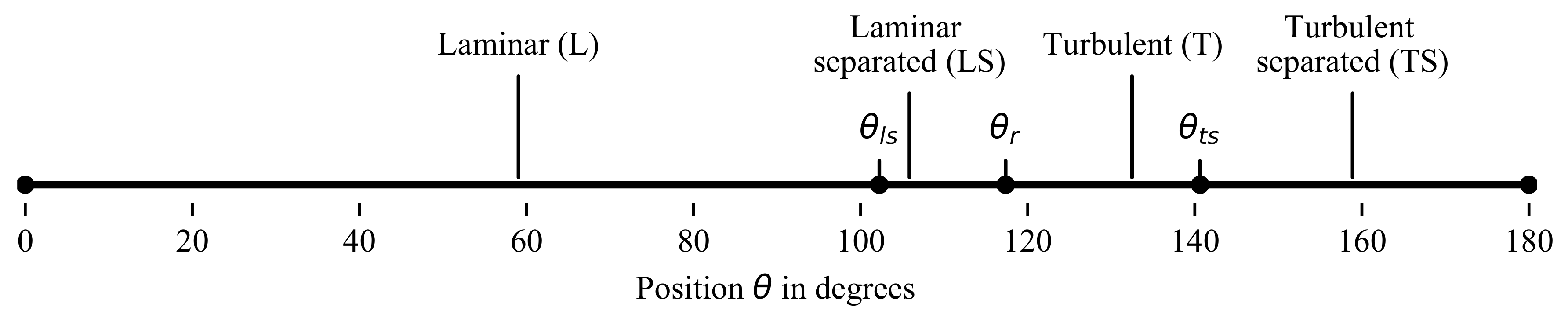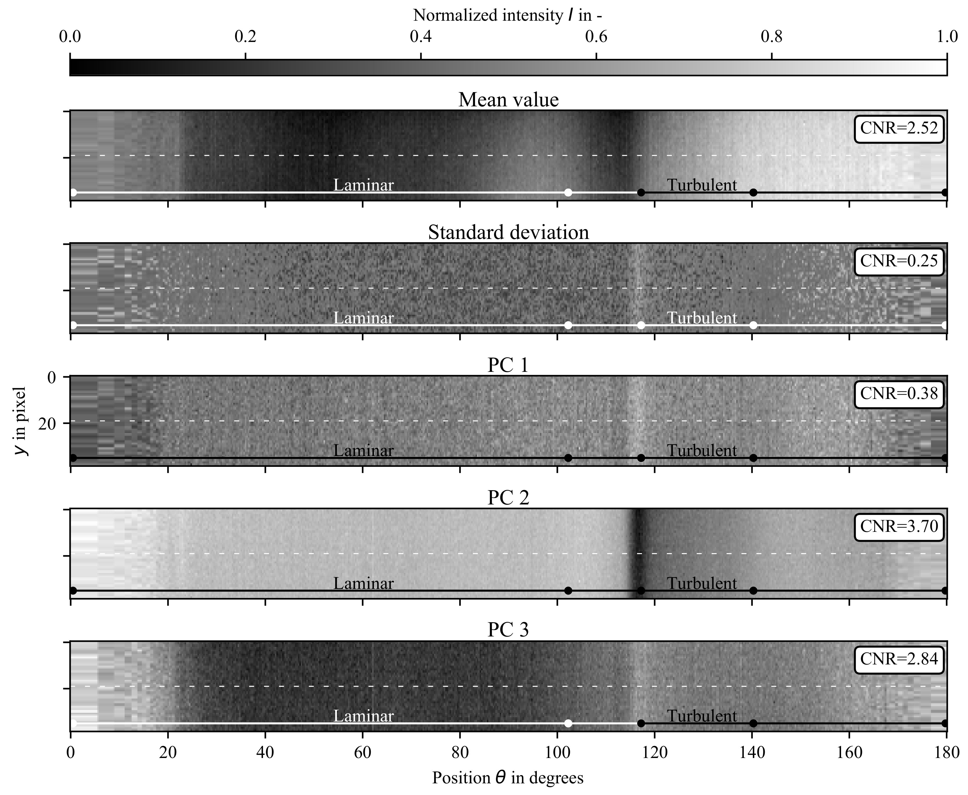The selected freestream flow velocity is $v_{\infty }=50\mathrm{m}/{\mathrm{s}}^{-1}$, resulting in a Reynolds number of 5.1 × 10⁵. For this flow condition, the boundary layer flow over the cylinder consists of laminar, turbulent and separated flow regimes as well as a laminar separation bubble in the region of laminar-turbulent flow transition, see Figure 3.

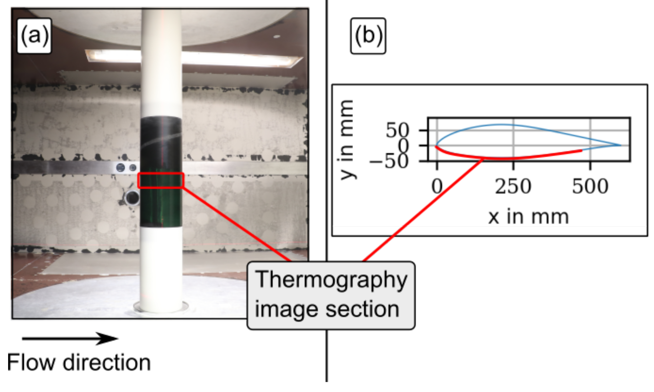
In order to study a measurement object equivalent to the perspective application on wind turbine rotor blades, a second experiment is conducted with a DU96W180 airfoil, see Figure 2b, with a chord length of 600 $\mathrm{m}$$\mathrm{m}$ and the same material properties as a real rotor blade airfoil. The flow velocities in two test cases are chosen to yield Reynolds numbers that are typical for the flow situation on wind turbines in operation, $\mathrm{Re}=2\times {10}^6$ for test case 1 and $\mathrm{Re}=3\times {10}^6$ for test case 2. Note further that all measurements are conducted with no explicit heating that could enhance the thermal contrast between the flow regimes. Therefore, the thermographic images are similar to in-process measurements on wind turbines in operation where the thermal conditions of surface and fluid cannot be manipulated easily. The existing thermal contrast between the fluid and surface in the wind tunnel experiments solely depends on the heating of the fluid by the wind tunnel fans and wall friction. The increase in the fluid temperature during test case 1 and test case 2 are $\mathrm{d}{T}_1/\mathrm{d}t=1.9\times {10}^{-5}\mathrm{K}{\mathrm{s}}^{-1}$ and $\mathrm{d}{T}_2/\mathrm{d}t=3.5\times {10}^{-4}\mathrm{K}{\mathrm{s}}^{-1}$, respectively. The angle of attack of the airfoil model in both test cases is $\alpha =$ 6^∘.

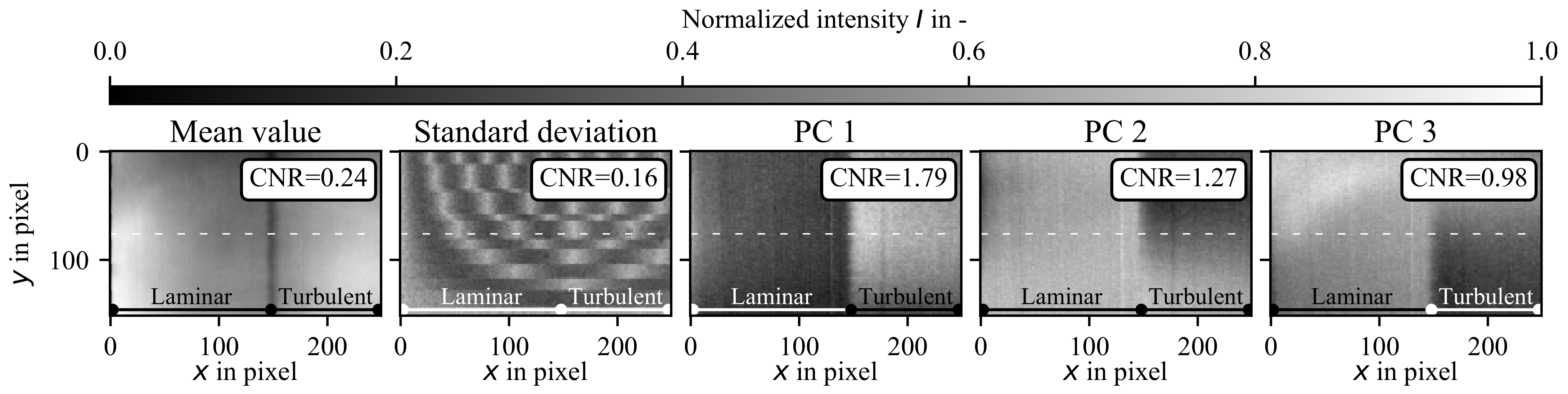
The two different heating rates result in different thermal conditions in the test cases 1 and 2. The mean surface temperature of the airfoil measurement object during test case 1 is in an almost steady state and increases during the image acquisition by only $\mathrm{d}{T}_1=0.02\mathrm{K}$. During test case 2 a transient state with a constant heating up increases the mean surface temperature by $\mathrm{d}{T}_2=0.35{}^{\circ }\mathrm{C}$. For the thermographic raw images this means that the thermal contrast between the laminar and turbulent flow regime in test case 1 is very low compared to the contrast in test case 2.

Additionally, an external heating source is used to create a disturbing reflection near the leading edge of the airfoil in test case 2. The reflection in combination with a flow-depending non-constant heat flux generates a non-homogenous temperature field within the laminar flow regime. This way the PCA can be examined for its ability to reduce systematic gradients in order to increase the distinguishability, when the thermal contrast in the thermographic image is already high.

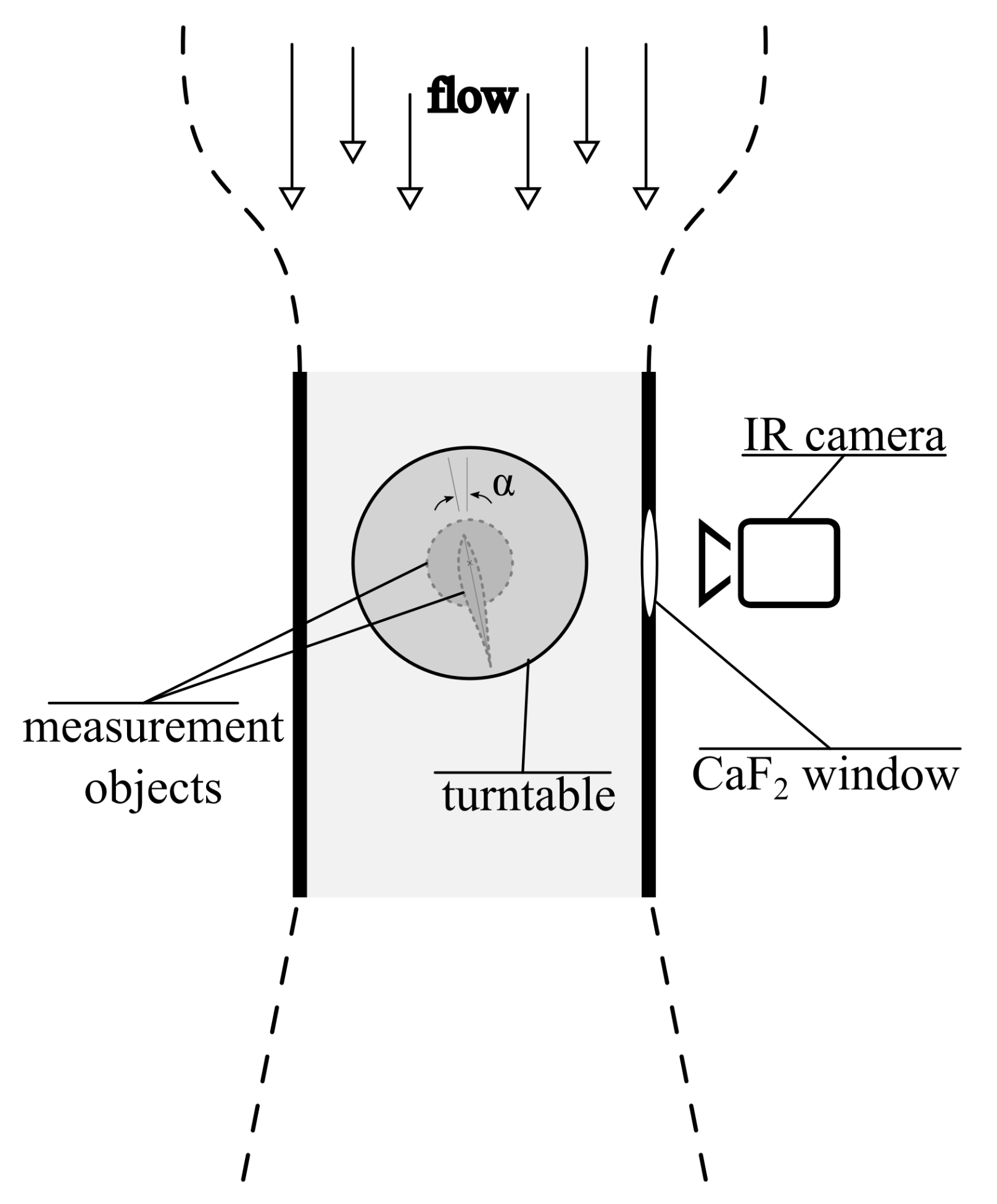
3.2. Thermographic Measurement System

The acquisition of the thermographic images is conducted with an infrared camera, typeImageIR 8300, from the manufacturer InfraTec. The actively cooled InSb focal plane array works with a global shutter (snap-shot detector), has a pixel size of 15 $\mathsf{\mu }$m at a full range resolution of 640 px × 512 px and a maximum frame rate of $100\mathrm{Hz}$ with an integration time set to 1600 $\mathsf{\mu }$s. The sensitivity is between 2.0 and 5.0 μm and has a noise equivalent temperature difference (NETD) of less than 25 mK @ 30 ${}^{\circ }\mathrm{C}$. The experimental setup is depicted in Figure 4. At a viewing distance of $1.75$ m and instantaneous field of view of $0.15$ mrad, a geometric resolution of $0.26$ mm results on the surface per pixel. An image series of the static flow situation is acquired with 6000 images for the cylinder and 10,000 images for the airfoil measurements, respectively. The image processing of the thermographic images is conducted with the script language Python.

3.3. Experiment Procedure

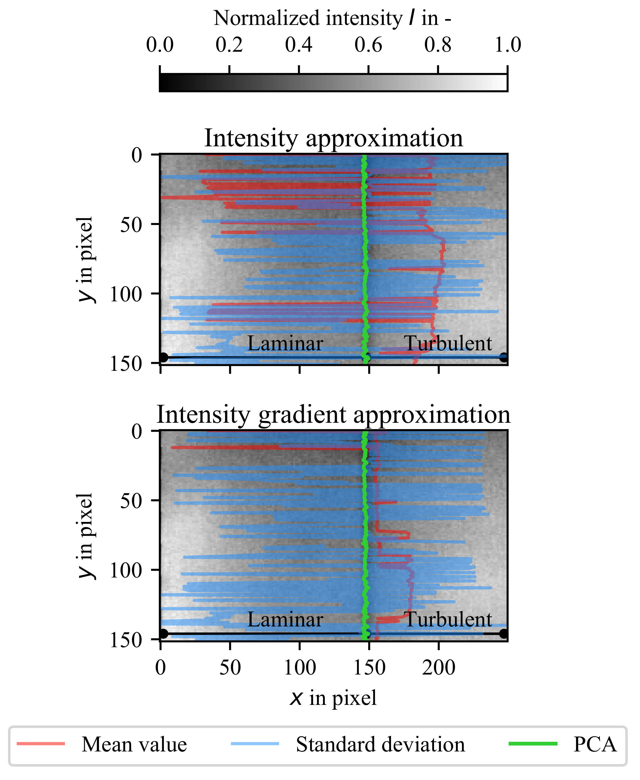
First, the thermographic images acquired by the cylinder measurements and the two airfoil test cases are pre-processed by separating the objects’ surface from the background in each image. For the measurement on the cylinder object, all images in the image series are rectified, and the areas in the two-dimensional image plane (640 px × 39 px) are allocated to the angular values $\theta =0{}^{\circ }$ to $\theta =180{}^{\circ }$ between the stagnation point and the opposite point on the cylinder object. The images of the two airfoil measurements are additionally cropped between the leading edge and the end of the turbulent flow regime, as the focus of this work is the distinguishability between these flow regimes, and surface modifications downstream create thermal artefacts that are not addressed in this work. The images have a dimensionality of 250 px × 152 px. In order to quantify the flow transition location normalized to the chord, the chord length c is calculated prior the cropping of the images.

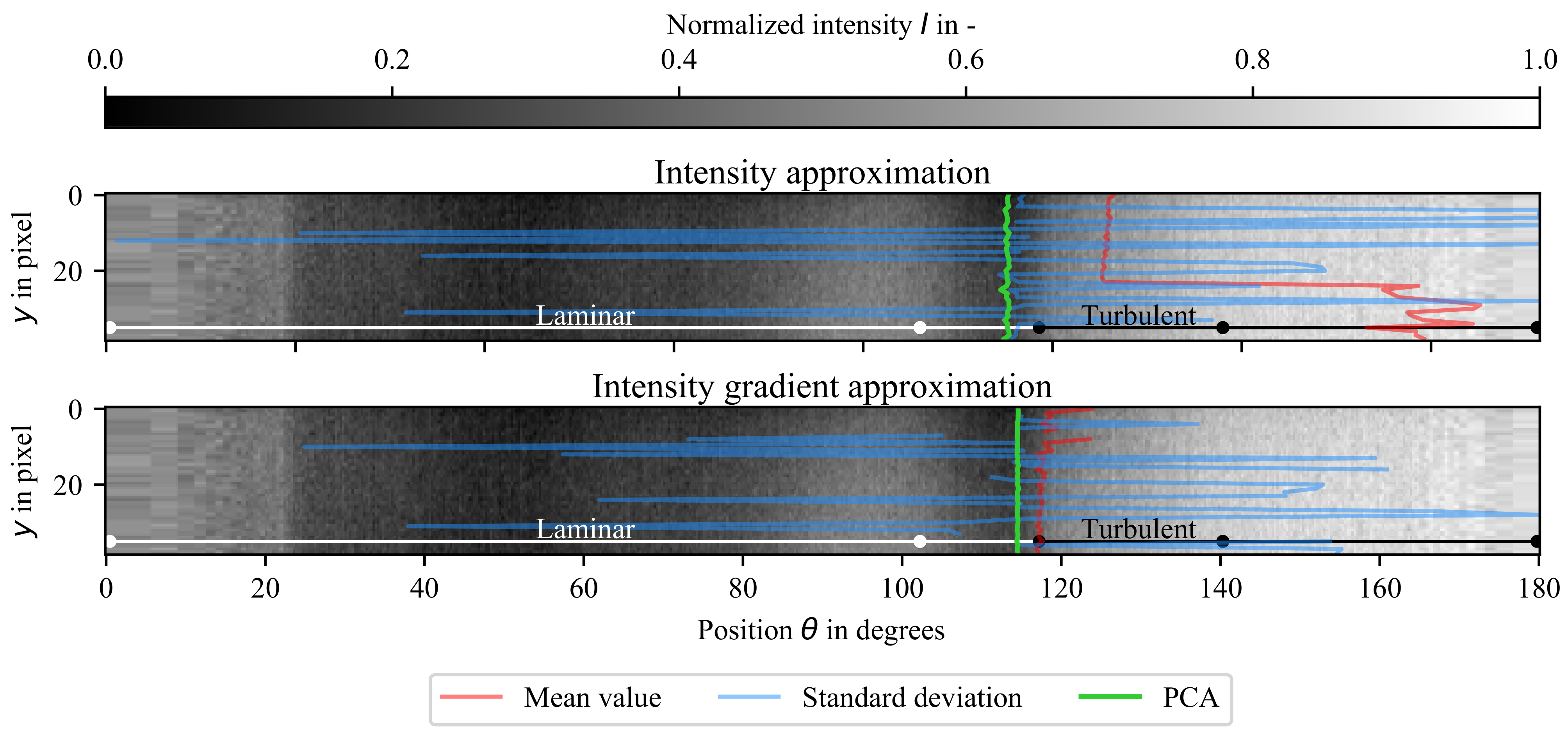
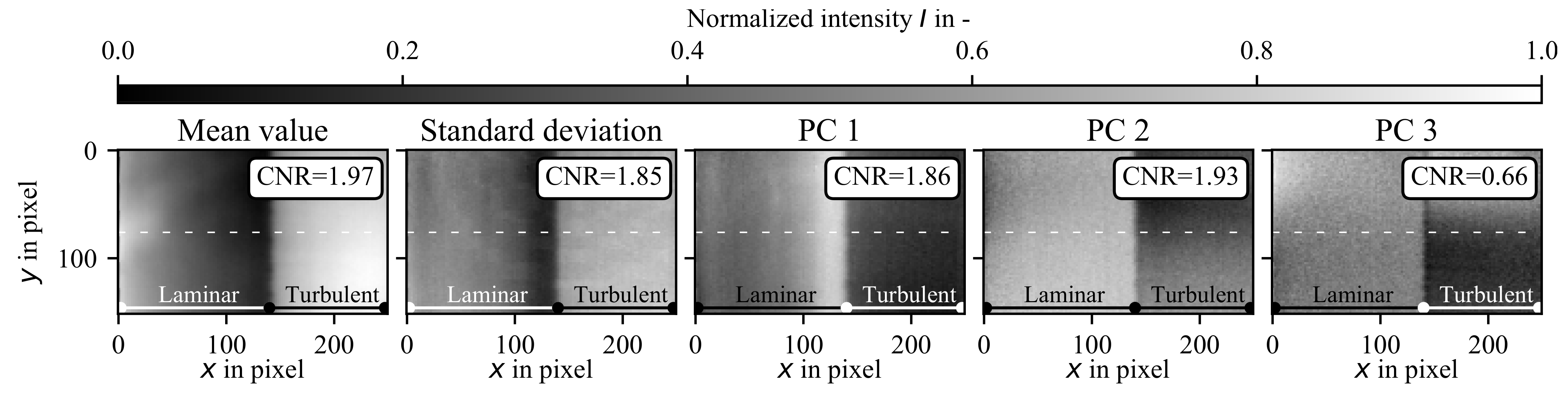
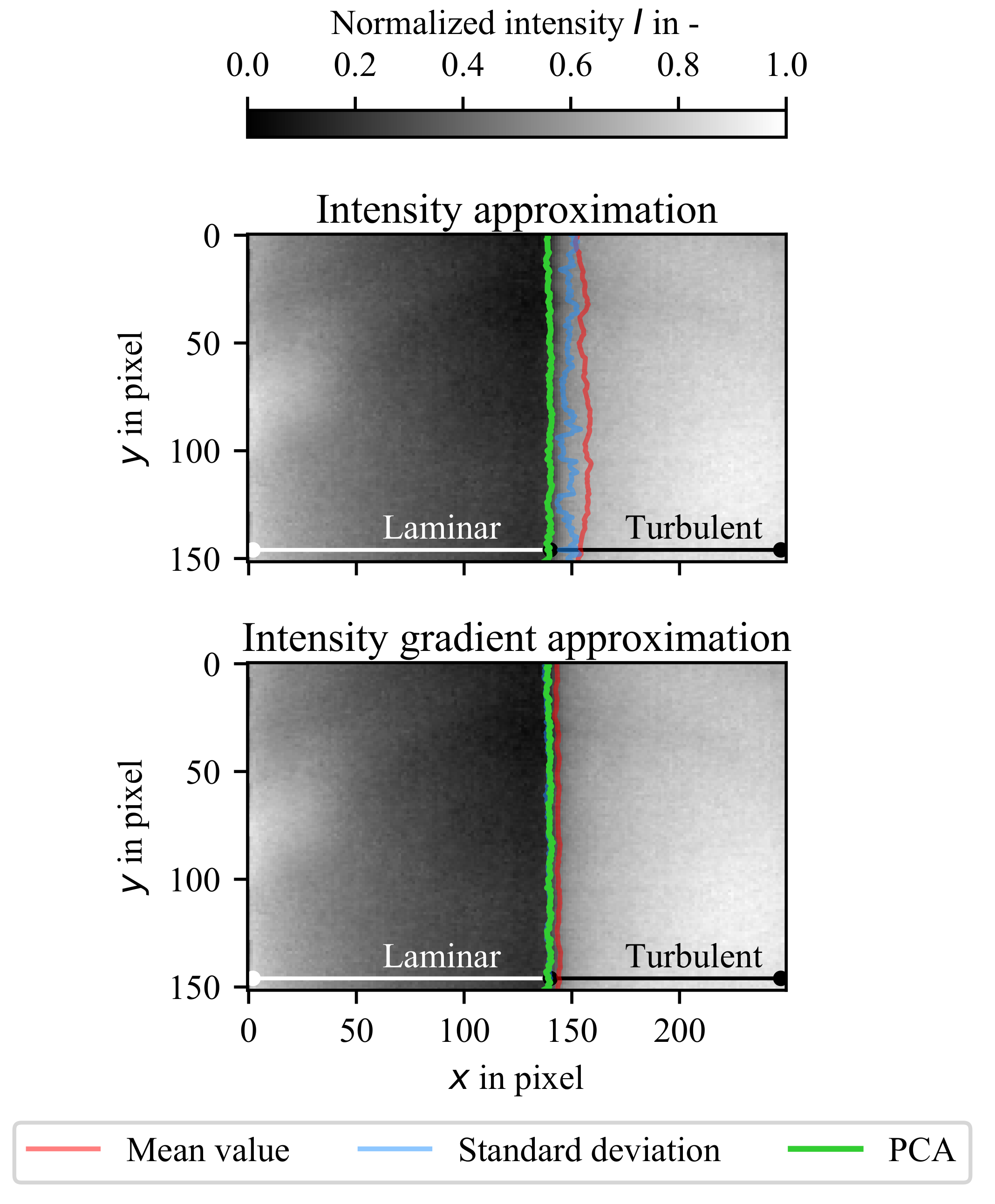
The images of all three experiments are afterwards evaluated by the PCA, and the PC images are calculated. To compare the PCA with classical image processing methods for creating flow visualizations, two additional methods are chosen. Firstly, the temporal mean value of the image series is considered as it is particularly successful in reducing white measurement noise and, therefore, increasing the CNR between different flow regimes. Secondly, the temporal standard deviation of the image series is considered because of its capability to reduce reflections and systematic gradients. The resulting flow visualizations of the PCA-based and the two classical image processing methods are compared with regard to the distinguishability between the laminar and turbulent flow regime quantified by the CNR, see Section 2.2. Additionally, all three flow visualizations are evaluated and compared concerning the systematic and random error of the flow transition localization conducted with both the Gaussian and Gaussian error fit methods. By assessing the different advantages of either image processing and flow localization method, the question how the PCA can be used as a complementary method to classical evaluations is studied.

4. Results

The following section presents the results of the PCA and compares the resulting flow visualizations with the two classical image processing methods. First, the temporal mean value, the temporal standard deviation and the first three PCs (PC 1, PC 2, PC 3) of each set of measurement images are shown in order to compare the flow visualizations qualitatively. Secondly, the intensity profiles in flow direction, the corresponding gradient and their approximations with the model functions from Equations (3) and (4), respectively, for locating the laminar-turbulent flow transition are presented for each flow visualization. Lastly, the located transition lines are compared with regard to their random and systematic measurement errors. The section is structured into three subsections: one for the cylinder and two for the two test cases with the airfoil.

4.1. Cylinder

Due to the changing incidence angle between the infrared camera and the curved surface of the cylinder object at the front and back, the radiation of the surface area in the out most left and right of the image plane is visualized as higher, as it can be explained by the surface temperature. This is due to the reflection of the environment and is consequently the result of a measurement artefact and will not be evaluated.

4.1.1. Flow Visualization

The flow visualizations resulting from the three image processing methods—temporal mean value, temporal standard deviation and PCA—are depicted in Figure 5. The extent of the laminar and turbulent flow regimes is marked in each image. The evaluation of the mean value shows the existing temperature gradients within the laminar and turbulent flow regimes due to the chord-position dependency of the friction coefficient and, thus, heat flux [1,5,10]. Additionally, the area in the middle of the image at the end of the laminar flow regime is superimposed with a reflection from the camera lens. The complete image also has random temperature fluctuations due to flow irregularities and measurement noise. Nevertheless, a qualitative distinguishability between the flow regimes is possible due to different intensities in the image.

The temporal standard deviation of the image series, shown in Figure 5, has almost no distinguishability between the flow regimes. However the artefact of the camera lens reflection is filtered out. While the flow regimes look more homogenous, the contrast between the flow regimes is low.

The PC 1 to PC 3 show great differences between each other. Note that the region of the reattachment of the laminar flow at ${\theta }_{\mathrm{r}}=117{}^{\circ }$ is emphasized in each image, due to its spatial fluctuation. Additionally, the systematic gradient within the laminar flow regime is reduced in each PC compared to the mean value, including the impact of the reflecting camera lens. However, a qualitative distinguishability between the laminar and turbulent flow regime seems only possible in PC 2 and PC 3.

The calculated CNR between the laminar and turbulent flow regimes is given in the top right corner of each image and reads $2.52$ for the mean value. Note that the camera lens reflection in the mean value image is not included in the CNR calculation in order to exclude the effect of the artefact. The PC 2 has the maximal CNR with $3.70$.

4.1.2. Flow Transition Localization

Figure 6 shows the intensity profile (blue) and the intensity gradient profile (orange) of the center row (white dashed line) of each flow visualization image from Figure 5. The approximation result for each profile is shown with a dashed line in the corresponding color. The flow transition position derived from the approximations is marked with a vertical dotted line.

The intensity profile of the temporal mean value shows the impact of the systematic temperature gradient within the laminar flow regime between $60{}^{\circ }<\theta <110{}^{\circ }$ and in the turbulent flow regime between $117{}^{\circ }<\theta <145{}^{\circ }$. Due to the course of the intensity profile, the approximation does not fit to the profile outside the turbulent flow regime. Because of this, the approximation curve does not center itself between the laminar and turbulent flow regimes and results in an estimated flow transition position within the turbulent flow regime. In addition, there is no sharp jump in intensity between the flow regimes, but a continuous steady increase that causes a flat slope of the approximation curve. The approximation of the intensity gradient profile fits to the gradient peak at $\theta \approx 118{}^{\circ }$ instead of centering between the laminar and turbulent flow regimes. This is due to the different systematic gradients in the flow visualization and the absence of a single prominent gradient peak between the flow regimes.

The intensity profile of the temporal standard deviation does not have two distinct plateaus representing the laminar and turbulent flow regime. The approximation therefore fails to fit to the profile correctly and has a high systematic error in the localization of the flow transition. The intensity gradient, however, has a prominent peak between the laminar and turbulent flow regime, allowing for a more accurate localization of the flow transition.

The intensity evaluation of the PC 2 illustrates the advantageous of the enhanced image processing by means of the PCA. Two distinct intensity plateaus are present due to the high CNR, while a sharper gradient between the laminar and turbulent flow regime persists. As a result, the approximations of the intensity profile as well as of the corresponding gradient profile successfully locate the flow transition between the laminar and turbulent flow regimes with a minimal error to the center position between them.

In order to compare the results of the located flow transition line in the entire flow visualization, the two introduced localization methods were repeated for each row of the temporal mean value, temporal standard deviation and PC 2 flow visualization image in Figure 5. The localization results are shown in Figure 7 with a single thermographic raw image as background and the located flow transition lines plotted in red for the mean value, blue for the temporal standard deviation and green for the PCA flow visualization result.

A comparison shows that the locations of the flow transition lines in the flow visualizations based on the two classical methods have a higher random and systematic error than those in the results based on the PCA. Consequently, the lowest systematic error ${\sigma }_{\mathrm{syst}}$ for either localization method in any of the classical image processing flow transitions amounts to $8.{33}^{\circ }$ for the intensity gradient approximation of the mean value, while the localization based on the intensity approximation in the PCA is the lowest with $3.{58}^{\circ }$. The random error ${\sigma }_{\mathrm{rand}}$ of the PCA result is also lower than in the classical methods with $0.{06}^{\circ }$. The minimal random error in any of the classical methods’ flow visualizations is $1.{24}^{\circ }$ for the approximation of the intensity gradient of the mean value. An overview over all errors is given in table

Table 1. Located flow transition position ${\theta }_{\mathrm{tr}}$ and corresponding random and systematic error ${\sigma }_{\mathrm{rand}}$ and ${\sigma }_{\mathrm{syst}}$ by means of both localizations methods for each image processing methods’ resulting flow visualization in the cylinder object experiment at a $\mathrm{Re}=5.1\times {10}^5$. Temporal mean value (mean), temporal standard deviation (std) and PCA. All values are normalized to the angular position [$0{}^{\circ },180{}^{\circ }$] on the cylinder.

	${\mathit{\theta }}_{\mathbf{tr}}$ in ${}^{\circ }$			${\mathit{\sigma }}_{\mathbf{rand}}$ in ${}^{\circ }$			${\mathit{\sigma }}_{\mathbf{syst}}$ in ${}^{\circ }$
	Mean	std	PCA	Mean	std	PCA	Mean	std	PCA
Intensity approximation	140.7	119.4	113.1	10.78	39.84	0.22	31.26	9.93	3.58
Intensity gradient approximation	117.8	118.6	114.4	1.24	34.14	0.06	8.33	9.59	4.89

.

To conclude, the PCA image processing is able to create a flow visualization with an increased CNR between the laminar and turbulent flow regime that maximizes the global distinguishability. As a result, the approximation of the intensity profile as well as the intensity gradient profile are able to auto-position themselves around the flow transition and minimize the systematic error of the flow transition localization in the PCA result. Additionally, the steep intensity step between the flow regimes is increased in the PCA-based flow visualization, minimizing the random error of the flow transition localization with both localization methods. The PCA image processing therefore enables a more robust flow transition localization in the considered measurement configuration.

4.2. DU96W180 Airfoil (Test Case 1)

4.2.1. Flow Visualization

The first test case on the DU96W180 airfoil is conducted at a chord Reynolds number of 2 × 10⁶. Due to the low flow velocity at the time of the image acquisition, the object surface is in a thermal equilibrium and does not change its temperature throughout the measurement. As a result, the contrast between the laminar and turbulent flow regime is very low. The flow visualization results by means of the PCA and the two classical image processing methods, the temporal mean value and the temporal standard deviation of the image series, are depicted in Figure 8. The only distinct feature in the mean value is a small area between both flow regimes with lower intensity, indicating a laminar separation bubble due to its effect of isolating the surface from the warmer fluid temperature. It is hardly possible to distinguish globally between the laminar and turbulent flow, since both areas have an almost equal intensity, and systematic gradients create inhomogeneities within both flow regimes.

The temporal standard deviation image does not show any flow features and consists only of noise and artefacts in the form of a circular pattern and a row-wise pattern, probably due to the camera lens and acquisition method. As no flow features are visible, a global distinguishability between the laminar and turbulent flow regime is not possible.

All three PCs show two distinct areas of different intensities, correlating with the laminar and turbulent flow regimes. However, the intensity as well as the contrast between the flow regimes varies in each image. On top of that, PC 3 shows an emphasized region in the top left that is likely to be traced back to an artefact caused by the camera lens. PC 1 and PC 2 do not inherit this artefact, though PC 2 shows a strong systematic gradient in the vertical direction. A qualitative inspection suggests that a global distinguishability between the laminar and turbulent flow regime is maximal in the PC 1.

The quantification of the CNR between the laminar and turbulent flow regimes in each flow visualization supports these observations. Without considering the temporal standard deviation, the mean value has the lowest CNR with 0.24, while all PC images have a higher CNR, and the maximum is found in PC 1 with 1.79.

4.2.2. Flow Transition Localization

Figure 9 shows the intensity profiles (blue) and respective intensity gradient profiles (orange) along the white dashed line depicted in the respective flow visualizations from Figure 8. The approximations of the intensity profiles and the gradient profiles are shown with a dashed line in the respective color. The results of each of the two flow transition localization methods are marked with a vertical dotted line.

As mentioned before, the temporal standard deviation flow visualization offers no features that can distinguish flow regimes. This is confirmed by the intensity and the intensity gradient profiles shown in Figure 9, as no distinct plateaus or single gradient peaks exist, respectively. The flow transition localization therefore has a high systematic error.

As expected by the low CNR between the flow regimes, no distinct plateaus with different intensities exist in the mean value. Consequently, the auto-positioning of the approximation fails, and the fitting curve does not center at the position of the flow transition. The intensity gradient profile has multiple peaks and no constant plateau around the flow transition, also resulting in a false positioning of the respective approximation. As a result, both methods have a high systematic error in the located position of the flow transition. Without a sharp temperature rise in the intensity profile and multiple peaks in the gradient profile, the random error is also expected to be high.

In the PC 1 flow visualization, however, two distinct plateaus in the intensity profile exist, as expected by the high CNR. Therefore, the approximation successfully auto-positions at the position of the flow transition between these plateaus with a minimal systematic error. Additionally, the steep intensity step between the flow regimes, visible as a high distinct peak in the intensity gradient profile, minimizes the random error and allows for an approximation of the intensity gradient profile with minimal systematic and random error. A comparison of the two intensity profiles and the intensity gradient profiles of the mean value and the PC 1 highlights the advantage of the PCA method for creating flow visualizations with two distinct intensity plateaus representing the two flow regimes and a steep step between them.

Figure 10 compares the results of the two flow transition localization methods applied to all image rows of the temporal mean value, temporal standard deviation and PC 1 flow visualizations depicted in Figure 8. The flow transition line results located in the mean value image are plotted in red, the ones from the temporal standard deviation image in blue and from the PCA image in green. As a background image, one single thermographic raw image from the image series is used.

A clear difference in the systematic and random localization errors between the PCA result and the two classical image processing methods is visible. Only the PCA result resembles the expected linear form of the flow transition line. The estimated systematic error ${\sigma }_{\mathrm{syst}}$ reads 0.34% and 0.30% the chord length c for the approximation method of the intensity and the intensity gradient profile, respectively. In comparison, the minimal systematic error in any of the classical image processing methods is achieved by the intensity gradient approximation in the mean value with 4.28% c. The same applies for the random error that reads 0.24% c for the intensity gradient approximation in the PCA result and 5.50% c for the same localization method in the mean value flow visualization. All measurement errors are listed in

Table 2. Located flow transition position $x_{\mathrm{tr}}$ and corresponding random and systematic error ${\sigma }_{\mathrm{rand}}$ and ${\sigma }_{\mathrm{syst}}$ by means of both localizations methods for each image processing methods’ resulting flow visualization in the DU96W180 test case 1 at a $\mathrm{Re}=2\times {10}^6$. Temporal mean value (mean), temporal standard deviation (std) and PCA. All values are normalized to the chord length c.

	${\mathit{x}}_{\mathbf{tr}}/\mathit{c}$ in %			${\mathit{\sigma }}_{\mathbf{rand}}/\mathit{c}$ in %			${\mathit{\sigma }}_{\mathbf{syst}}/\mathit{c}$ in %
	Mean	std	PCA	Mean	std	PCA	Mean	std	PCA
Intensity approximation	53.1	40.9	46.1	17.62	22.07	0.25	6.96	7.08	0.34
Intensity gradient approximation	50.7	41.0	46.1	5.50	23.00	0.24	4.28	5.51	0.30

.

To conclude, when the fluid temperature is nearly constant during the measurement, and the contrast between the laminar and turbulent flow regime is low, the PCA enables not only an increase in distinguishability but also a flow transition localization with minimal random and systematic error.

4.3. DU96W180 Airfoil (Test Case 2)

4.3.1. Flow Visualization

The second test case on the DU96W180 airfoil was conducted at a chord Reynolds number of 3 × 10⁶. The fluid during the experiment has a positive temporal temperature gradient caused by the higher flow velocity, see Section 3.1, resulting in a constant heating of the airfoil. Due to different heat coefficients in the laminar and turbulent flow regimes, both regimes have a different temporal temperature gradient. As a result, the two classical image processing methods’ flow visualizations, the temporal mean value and the temporal standard deviation of the image series, shown in Figure 11, have a high CNR between the flow regimes of 1.97 and 1.85, respectively. In both images, a clear distinguishability between the two flow regimes is possible.

The PCA flow visualizations for PC 1 to PC 3 also have a good contrast between the flow regimes; however, differences in the reduction in spatial temperature gradients within the flow regimes exist. The PC 1, for example, has a gradient within the laminar flow regime just as strong as the mean value or the standard deviation image. The most homogenous flow regime, by sufficient contrast, is located in PC 2 with a CNR of 1.93. The global contrast was not increased by the PCA evaluation compared to the classical methods, but spatial gradients are reduced due to the flow as well as artefacts such as the reflection on the left side of the image, increasing the homogeneity of the flow regimes.

4.3.2. Flow Transition Localization

Figure 12 shows the intensity profile, intensity gradient profile, the approximations for locating the flow transition as well as the resulting flow transition positions equivalent to the last section, see Section 4.2. All intensity profiles have a high gradient at $x\approx 148\mathrm{px}$ that enables a flow transition localization with minimal random error with either localization method. However, the systematic gradients within the laminar flow regimes in both the mean value and the temporal standard deviation have the effect that no distinct intensity plateaus representing the two flow regimes exist. As a consequence, the approximation of the intensity does not auto-center at the position of flow transition, resulting in a systematic error of the localization. In the PC flow visualization, however, the reduction in the systematic gradients lead to the existence of two clearly distinct intensity plateaus between which the intensity approximation successfully centers.

Figure 13 shows the result of the entire flow transition line localization over all image rows based on the temporal mean value (red), the temporal standard deviation (blue) and the PCA (green) result. Due to the high gradient at the position of the flow transition, the localization by means of the intensity gradient approximation has minimal random and systematic error in each flow visualization. The spatial temperature gradient in the laminar flow regime due to the changing heat flux and thermal reflection in the mean value and the temporal standard deviation results in a higher systematic error compared to the PCA result if the flow transition is located by means of the intensity profile approximation. Nonetheless, the minimal random error ${\sigma }_{\mathrm{rand}}$ and systematic error ${\sigma }_{\mathrm{syst}}$ amount to 0.13% c and 0.52% c for the approximation of the intensity gradient profile in the mean value. All errors are listed in

Table 3. Located flow transition position $x_{\mathrm{tr}}$ and corresponding random and systematic error ${\sigma }_{\mathrm{rand}}$ and ${\sigma }_{\mathrm{syst}}$ by means of both localization methods for each image processing method’s resulting flow visualization from the DU96W180 test case 2 at a $\mathrm{Re}=3\times {10}^6$. Temporal mean value (mean), temporal standard deviation (std) and PCA. All values are normalized to the chord length c.

	${\mathit{x}}_{\mathbf{tr}}/\mathit{c}$ in %			${\mathit{\sigma }}_{\mathbf{rand}}/\mathit{c}$ in %			${\mathit{\sigma }}_{\mathbf{syst}}/\mathit{c}$ in %
	Mean	std	PCA	Mean	std	PCA	Mean	std	PCA
Intensity approximation	48.9	46.6	43.8	0.50	0.74	0.21	4.36	2.05	0.75
Intensity gradient approximation	45.0	43.6	43.8	0.13	0.17	0.20	0.52	0.93	0.76

.

In conclusion, the PCA is able to reduce the influence of systematic gradients within the flow regimes due to reflection artefacts or spatial temperature gradients, allowing for a flow transition localization with the approximation of the intensity profile. However, the random and systematic errors for an approximation of the intensity gradient profile are on the same order of magnitude for each image processing method. Only if the approximation of the intensity is preferred does the PCA have advantages for locating the flow transition with reduced errors.

5. Conclusions and Outlook

The article introduced an enhanced image processing method based on PCA for the thermographic flow visualization of wind turbine rotor blades. The goal was to increase the distinguishability between the laminar and turbulent flow regimes and finally enabling a flow transition localization with minimal random and systematic error. The PCA results are compared to two classical image processing methods for evaluating a thermographic image series: the temporal mean value and the temporal standard deviation. Furthermore, two flow transition localization methods were introduced based on the approximation of the intensity profile and the intensity gradient profile in flow direction with a Gaussian error function and Gaussian function, respectively.

The evaluation was applied to a cylinder in cross-flow condition and a DU96W180 airfoil. This allowed the study on a well-known geometry in fluid dynamics by means of the cylinder as well as on a more application-oriented object. The experiments were conducted in a wind tunnel with a closed test section and Reynolds numbers oriented on the application on real wind turbines. For the airfoil, two different fluid temperature situations were tested. A steady-state test case with an almost constant fluid temperature and a transient state with a positive temperature gradient were evaluated during the experiment. In this way, it was possible to analyze the PCA results on thermographic images with little to no distinguishability between the laminar and turbulent flow regimes and images with a high initial distinguishability. Thus, all possibilities from the real application were covered, and the potential of PCA regarding the application on wind turbines in operation was studied.

In the cylinder experiment, the PCA enables a more robust localization of the flow transition compared to the classical image processing methods. The effects of systematic gradients and artefacts are minimized, and the CNR is increased by 47%. The random error of the localization is reduced by a factor of 20.7 and the systematic error by 57%. In test case 1 with a low contrast between flow regimes, the classical methods are not able to increase the CNR. Applying the PCA, however, a flow visualization with an increased CNR by a factor of 7.5 is created, and the systematic and random measurement errors of the flow transition localization are reduced by 3.98% and 5.26% of the chord length c, respectively. If the distinguishability is already high, the PCA achieves a CNR on the same order of magnitude as the classical methods. However, the PCA enables a more robust flow transition localization by means of the intensity profile approximation with a Gaussian error function, as spatial systematic gradients in the flow regimes are reduced. The first airfoil test case also shows that the existence of a laminar separation bubble highly influenced the localization in the classical image processing methods, while the PCA result is unaffected and allows for a more robust flow transition localization.

The increase in the flow regimes’ distinguishability for measurement conditions with a low initial temperature difference between fluid and surface minimizes the requirement of the thermographic flow visualization technique with regard to the necessary solar energy input. Being less dependent on the strong blade heating, measurements during cloudy days, early in the morning or late in the day become possible. Additionally, a flow transition localization with reduced errors improves the assessment of the aerodynamic condition of the wind turbine and the decision regarding the necessity of maintenance work. Note that the findings of this work are applicable to any similar setup with an airfoil in cross-flow condition and comparable Reynold’s numbers, for instance aircraft wings and helicopter blades [21].

Even if the introduced image processing methods evaluate different information in the image series, the combination of the methods does not prove to be advantageous. However, the surface area of the laminar and turbulent flow regimes was cropped from the background prior to the analysis, as the PCA is sensitive to any changes in the image series, including the background. For a pre-evaluation, the classical methods, such as the mean value of the image series, are more robust to identify the surface area and the rough distribution of the flow regimes. Afterwards a more detailed evaluation by the PCA is capable to maximize the distinguishability and minimize the measurement error of the flow transition localization. This way, the PCA is a valuable addition to the existing evaluation methods of thermographic images. With the absence of an artificial heating or cooling of the measurement object or the fluid, this work is capable for a future application to in-process measurements on wind turbines in operation.

Thus, the next step is conducting experiments on real wind turbines. For this task, a co-rotation of the measurement setup with the rotation of the rotor is desirable to acquire the image series with a high frequency. In addition, more wind tunnel experiments on the cross-sensitivities of the PCA on artefacts, dead pixels in the thermographic image or the pre-chopping of the image data need to be carried out. An analysis of the necessary number of images as well as the measurement frequency in order to achieve the increase in distinguishability could give information about the minimal necessary image acquisition effort. Additionally, a post-processing of the principal components should be developed in order to decide which component or which combination of components inherits the most information about the flow situation.

References

1. Schlichting, H. Boundary-Layer Theory; McGraw-Hill: New York, NY, USA, 1979. [Google Scholar]
2. Quast, A. Detection of Transition by Infrared Image Techniques. Tech. Soar. 2006, 30, 33–38. [Google Scholar]
3. Peake, D.J.; Bowker, A.J.; Lockyear, S.J.; Ellis, F. Non-obtrusive detection of transition region using an infra-red camera. In Proceedings of the AGARD Laminar-Turbulent Transition 17 P (SEE N78-14316 05-34, Lyngby, Denmark, 2–4 May 1977. [Google Scholar]
4. Bouchardy, A.M.; Durand, G. Processing Of Infrared Thermal Images For Aerodynamic Research. In Applications of Digital Image Processing V; Oosterlinck, A.J., Tescher, A.G., Eds.; SPIE: Geneva, Switzerland, 1983; pp. 304–309. [Google Scholar] [CrossRef]
5. de Luca, L.; Carlomagno, G.M.; Buresti, G. Boundary layer diagnostics by means of an infrared scanning radiometer. Exp. Fluids 1990, 9, 121–128. [Google Scholar] [CrossRef]
6. de Luca, L.; Guglieri, G.; Cardone, G.; Carlomagno, G.M. Experimental analysis of surface flow on a delta wing by infrared thermography. AIAA J. 1995, 33, 1510–1512. [Google Scholar] [CrossRef]
7. Gartenberg, E.; Johnson, W.G.; Wright, R.E.; Carraway, D.L.; Johnson, C.B. Boundary-layer transition-detection in a cryogenic wind tunnel using infrared imaging. AIAA J. 1992, 30, 444–446. [Google Scholar] [CrossRef]
8. Montelpare, S.; Ricci, R. A thermographic method to evaluate the local boundary layer separation phenomena on aerodynamic bodies operating at low Reynolds number. Int. J. Therm. Sci. 2004, 43, 315–329. [Google Scholar] [CrossRef]
9. Ricci, R.; Montelpare, S. Analysis of boundary layer separation phenomena by infrared thermography Use of acoustic and/or mechanical devices to avoid or reduce the laminar separation bubble effects. Quant. Infrared Thermogr. J. 2009, 6, 101–125. [Google Scholar] [CrossRef]
10. Gartenberg, E.; Roberts, A.S. Airfoil transition and separation studies using an infrared imaging system. J. Aircr. 1991, 28, 225–230. [Google Scholar] [CrossRef]
11. Dollinger, C. Thermografische Strömungsvisualiserung an Rotorblättern von Windenergieanlagen; Shaker Verlag: Düren, Germany, 2018. [Google Scholar]
12. Joseph, L.A.; Borgoltz, A.; Devenport, W. Infrared thermography for detection of laminar-turbulent transition in low-speed wind tunnel testing. Exp. Fluids 2016, 57, 77. [Google Scholar] [CrossRef]
13. Bæk, P.; Fuglsang, P. Experimental detection of transition on wind turbine airfoils. In Proceedings of the European Wind Energy Conference and Exhibition, Marseille, France, 16–19 March 2009; pp. 1628–1652. [Google Scholar]
14. Crawford, B.K.; Duncan, G.T.; West, D.E.; Saric, W.S. Robust, automated processing of IR thermography for quantitative boundary-layer transition measurements. Exp. Fluids 2015, 56, 149. [Google Scholar] [CrossRef] [Green Version]
15. Dollinger, C.; Balaresque, N.; Sorg, M.; Fischer, A. IR thermographic visualization of flow separation in applications with low thermal contrast. Infrared Phys. Technol. 2018, 88, 254–264. [Google Scholar] [CrossRef]
16. Gleichauf, D.; Dollinger, C.; Balaresque, N.; Gardner, A.D.; Sorg, M.; Fischer, A. Thermographic flow visualization by means of non-negative matrix factorization. Int. J. Heat Fluid Flow 2020, 82, 108528. [Google Scholar] [CrossRef]
17. Rajic, N. Principal component thermography for flaw contrast enhancement and flaw depth characterisation in composite structures. Compos. Struct. 2002, 58, 521–528. [Google Scholar] [CrossRef]
18. Traphan, D.; Meinlschmidt, P.; Schlüter, F.; Lutz, O.; Peinke, J.; Gülker, G. High-speed measurements of different laminar-turbulent transition phenomena on rotor blades by means of infrared thermography and stereoscopic PIV. In Proceedings of the 10th Pacific Symposium on Flow Visualization and Image Processing, Naples, Italy, 15–18 June 2015; p. 207. [Google Scholar]
19. Heineck, J.T.; Schülein, E.; Raffel, M. Boundary layer transition detection on a rotor blade using rotating mirror thermography. In Proceedings of the Fifth Decennial AHS Aeromechanics Specialists’ Conference, San Francisco, CA, USA, 22–24 January 2014. [Google Scholar]
20. Gleichauf, D.; Sorg, M.; Fischer, A. Contactless Localization of Premature Laminar–Turbulent Flow Transitions on Wind Turbine Rotor Blades in Operation. Appl. Sci. 2020, 10, 6552. [Google Scholar] [CrossRef]
21. Wolf, C.; Gardner, A.D.; Raffel, M. Infrared thermography for boundary layer transition measurements. Meas. Sci. Technol. 2020, 31, 112002. [Google Scholar] [CrossRef]
22. Dollinger, C.; Sorg, M.; Balaresque, N.; Fischer, A. Measurement uncertainty of IR thermographic flow visualization measurements for transition detection on wind turbines in operation. Exp. Therm. Fluid Sci. 2018, 97, 279–289. [Google Scholar] [CrossRef]
23. Hotelling, H. Analysis of a Complex of Statistical Variables into Principal Components; American Psychological Association (APA): Washington, DC, USA, 1933; Volume 24. [Google Scholar] [CrossRef]
24. Abdi, H.; Williams, L.J. Principal component analysis. Wiley Interdiscip. Rev. Comput. Stat. 2010, 2, 433–459. [Google Scholar] [CrossRef]
25. Wold, S.; Esbensen, K.; Geladi, P. Principal component analysis. Chemom. Intell. Lab. Syst. 1987, 2, 37–52. [Google Scholar] [CrossRef]
26. Does, M.D.; Olesen, J.L.; Harkins, K.D.; Serradas-Duarte, T.; Gochberg, D.F.; Jespersen, S.N.; Shemesh, N. Evaluation of principal component analysis image denoising on multi-exponential MRI relaxometry. Magn. Reson. Med. 2019. [Google Scholar] [CrossRef] [PubMed]
27. Chin, C.S.; Ji, X.; Woo, W.L.; Kwee, T.J.; Yang, W. Modified multiple generalized regression neural network models using fuzzy C-means with principal component analysis for noise prediction of offshore platform. Neural Comput. Appl. 2019, 31, 1127–1142. [Google Scholar] [CrossRef] [Green Version]
28. Turk, M.; Pentland, A. Eigenfaces for Recognition. J. Cogn. Neurosci. 1991, 3, 71–86. [Google Scholar] [CrossRef] [PubMed]
Figure 1. (a) Flow visualization image with a laminar and turbulent flow regime distinguishable by different intensity levels. (b) Intensity profile (thin black line) and intensity gradient profile (thin black dotted) along the white dashed line in (a). Two distinct intensity plateaus corresponding to the laminar and turbulent flow regime are visible with a steep change between them. A Gaussian error function fitted to the intensity profile is shown with a thick black line, and a Gaussian function fitted to the corresponding gradient profile is shown with a thick black dotted line. The laminar-turbulent flow transition can be localized by the saddle point of the Gaussian error function and by the maximum of the Gaussian function.
Applsci 11 05471 g001
Figure 2. Both measurement objects used in this work. (a) DU96W180 airfoil object with a chord length of 600 m m . (b) Cylinder object with a diameter of 160 m m in the wind tunnel test section.
Applsci 11 05471 g002
Figure 3. Oil paint measurement on a 160 m m diameter cylinder in cross-flow at a Reynolds number of Re = 5.1 × 10 5 . The beginning and end of the different boundary layer flow regimes is visible by the accumulation of oil.
Applsci 11 05471 g003
Figure 4. Experimental setup in the wind tunnel. The thermographic camera ImageIR 8300 watches the cylinder measurement object through a CaF 2 -window. Additional camera systems observe the test section of the wind turbine.
Applsci 11 05471 g004
Figure 5. Thermographic flow visualization of the cylinder object in cross-flow with a Reynolds number of 5.2 × 10⁵. Temporal mean value and temporal standard deviation as well as principal components (PC) no. 1–3 from the PCA of the image series. Systematic inhomogeneities in the flow regimes are reduced while a contrast between the laminar and turbulent flow regime is maximized in PC 2 with CNR = 3.70 .
Applsci 11 05471 g005
Figure 6. The intensity profile (blue line), intensity gradient profile (orange line) along the white dotted line in the temporal mean value, temporal standard deviation and PC 2 flow visualization in Figure 5. The approximation of the intensity profile (blue dashed) and intensity gradient profile (orange dashed), respectively. The flow transition localization results of both methods are depicted with a vertical dotted line in the respective color. Different expressions of the intensity plateaus are visible in each profile with varying gradient amplitudes between the plateaus. The most distinct expression of two plateaus including a steep step between them exists in the PC 2.
Applsci 11 05471 g006
Figure 7. Comparison of the located laminar turbulent flow transition line by means of the temporal mean value (red), temporal standard deviation (blue) and PCA (green) flow visualization of the image series. Flow transition localization based on the approximation of the intensity profile (top) and approximation of the intensity gradient profile (bottom). For both methods, the localization in the PCA result has qualitatively the lowest random and systematic error.
Applsci 11 05471 g007
Figure 8. Thermographic flow visualization of the DU96W180 airfoil in cross-flow with a Reynolds number of 2 × 10⁶. Temporal mean value and temporal standard deviation as well as principal components (PC) no. 1–3 from the PCA of the image series. Systematic inhomogeneities in the flow regimes are reduced while a contrast between the laminar and turbulent flow regime is maximized in PC 1 with CNR = 1.79 .
Applsci 11 05471 g008
Figure 9. The intensity profile (blue line), intensity gradient profile (orange line) along the white dotted line in the temporal mean value, temporal standard deviation and PC 1 flow visualization in Figure 8. The approximation of the intensity profile (blue dashed) and intensity gradient profile (orange dashed), respectively. The flow transition localization results of both methods are depicted with a vertical dotted line in the respective color. Different expressions of the intensity plateaus are visible in each profile with varying gradients between the plateaus. The most distinct expression of the two plateaus including a steep step between them exists in the PC 1.
Applsci 11 05471 g009
Figure 10. Comparison of the located laminar turbulent flow transition line by means of the temporal mean value (red), temporal standard deviation (blue) and PCA (green) flow visualization of the image series. Flow transition localization based on the approximation of the intensity profile (top) and approximation of the intensity gradient profile (bottom). For both methods, the localization in the PCA result has qualitatively the lowest random and systematic error.
Applsci 11 05471 g010
Figure 11. Thermographic flow visualization of the DU96W180 airfoil in cross-flow with a Reynolds number of 3 × 10⁶. Temporal mean value and temporal standard deviation as well as principal components (PC) no. 1–3 from the PCA of the image series. Systematic inhomogeneities in the flow regimes are reduced in the PC, while a contrast between the laminar and turbulent flow regime is maximized in the mean value with CNR = 1.79 .
Applsci 11 05471 g011
Figure 12. The intensity profile (blue line), intensity gradient profile (orange line) along the white dotted line in the temporal mean value, temporal standard deviation and PC 1 flow visualization in Figure 11. The approximation of the intensity profile (blue dashed) and intensity gradient profile (orange dashed), respectively. The flow transition localization results of both methods are depicted with a vertical dotted line in the respective color. Different expressions of the intensity plateaus are visible in each profile with varying gradient amplitudes between the plateaus. The most distinct expression of two plateaus including a steep step between them exists in the PC 2, even though the high gradient in the classical image processing result is sufficient for an auto-centering of the intensity gradient approximation.
Applsci 11 05471 g012
Figure 13. Comparison of the located laminar turbulent flow transition line by means of the temporal mean value (red), temporal standard deviation (blue) and PCA (green) flow visualization of the image series. Flow transition localization based on the approximation of the intensity profile (top) and approximation of the intensity gradient profile (bottom). The intensity gradient approximation method successfully locates the flow transition in each image with minimal random and systematic error due to the existence of a high gradient. The localization based on the intensity profile approximation in the classical image processing methods, however, has a larger systematic error. This error is minimized if the PC flow visualization is used for the localization.
Applsci 11 05471 g013