The Effect of Wind Energy on Microclimate: Lessons Learnt from a CFD Modelling Approach in the Case Study of Chios Island ^†

Abstract

During the last three decades, rapid growth of wind energy has led to questions regarding the possible impacts of wind farms on local weather and microclimates. Physically, the increased turbulence due to the wind turbine operation affects the mixing processes, may slightly disturb the pressure and temperature distributions downstream of wind farms and may have an impact on natural ecosystems such as the famous mastic tree population located on the island of Chios in the North Aegean Sea. This study explores the wind farms and their wake effects downstream with a particular focus on the effect on the southern part of the island where the mastic trees cultivation is located. The analysis is carried out with the use of the commercial CFD code ANSYS Fluent. Steady state computations of full 3D Navier–Stokes equations, using the k-ε turbulence closure scheme are carried out. The development of the multiple wake effects of the wind farms and their propagation downstream is examined under low and high turbulence intensities. Results clearly indicate that for both test cases there is no impact to the local microclimate and to the mastic Tree population.

Highlights

• CFD simulations of a large-scale wind farm using actuator disk models and Monin–Obukhov similarity theory for stable atmospheric stratification.
• Evaluation of the microclimate impact of a wind farm in Chios island by investigating the multiple wake effects length using a case scenario with low ambient TKE.
• The wind energy project under investigation will not affect the microclimate of the sensitive south part of Chios island and the mastic trees cultivation.

1. Introduction

The abundant wind potential across the Greek archipelago has led to many islands generating wind energy not only to their own needs but transmitting excess energy to the mainland via sub-sea cables, thereby increasing national energy security and contributing to the achievement of national goals for renewable energy. In all these cases, such developments must be planned considering other land uses and protected areas setting additional constraints to wind energy development. Over the last decade, Greece has faced a severe economic crisis that was in practice blocking and freezing even mature investments on wind energy. However, recently there is a growing market interest that opens the discussion over relevant socioeconomic and environmental topics. Currently, local authorities and communities are skeptical of large-scale wind farms due to fear that such projects could affect tourism, cultivations, local products, and, as a result, the sensitive local economy. Our work is contributing to the clarification of such misconceptions.

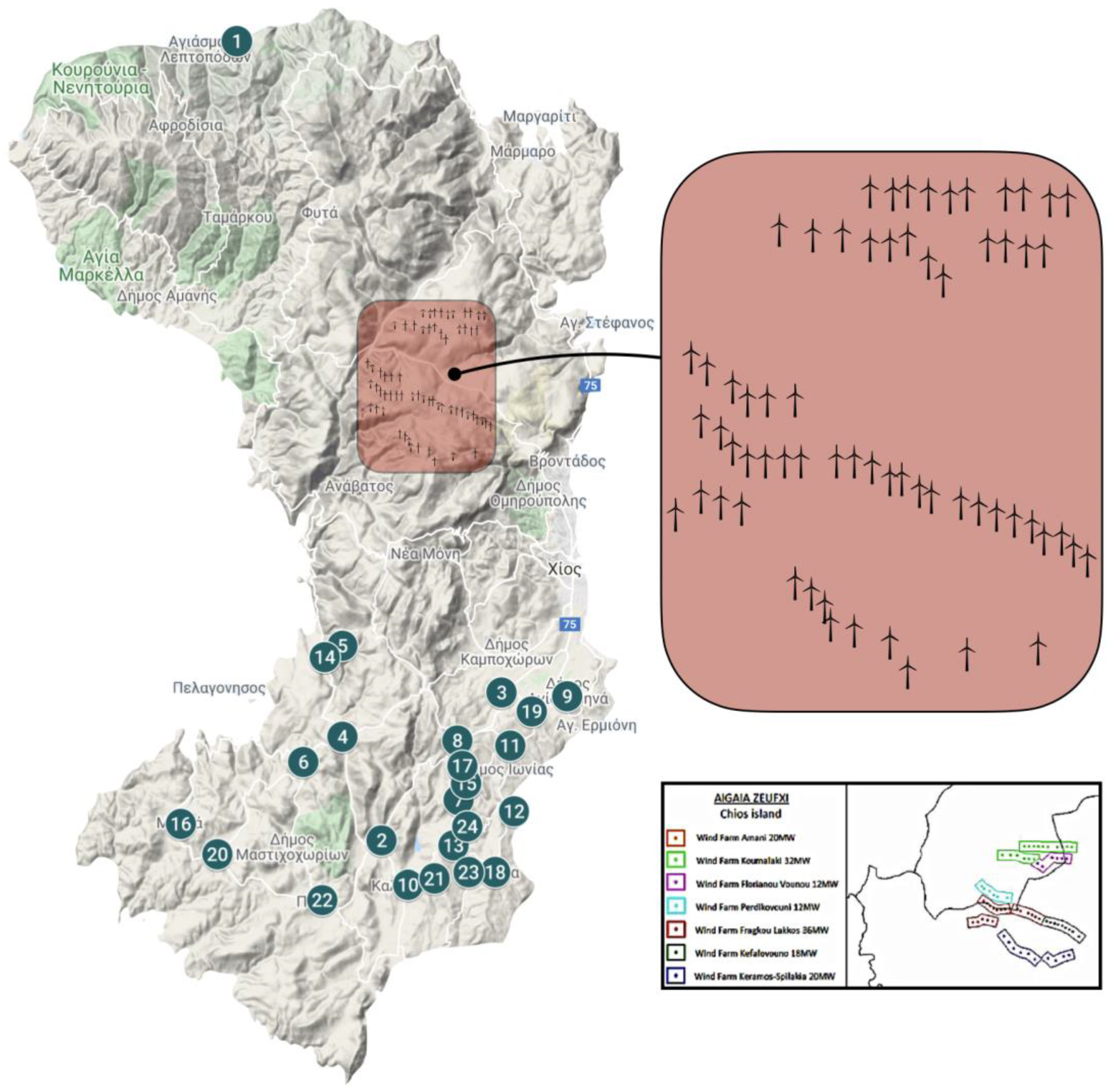
One of the first proposals for large scale wind integration projects in Greek islands was located at the islands of the North Aegean Sea, namely Lesvos, Limnos, and Chios with a cumulative wind capacity of 706 MW. More than 15 years later, this project has not yet been realized due to obstacles related to bureaucracy, local reactions, technical difficulties for the interconnection, etc. According to the project description, seven wind farms with a total capacity of 150 MW are to be installed in the island of Chios. The island of Chios is famous for the mastic trees cultivation located in the south part of the island. There is a fear amongst the local population that large scale wind energy development in Chios will affect the microclimate and especially the mastic trees cultivation.

A CFD modelling approach is used to examine the wake effects and their magnitude downstream of the proposed wind farms in the north part of the island. The island’s mastic production is controlled by a co-operative of medieval villages, collectively known as the “Mastichochoria”, located in southern Chios, 15 km downstream of the proposed wind farm’s location. To examine the wake effects and their interaction with the microclimate of the area, this investigation focuses on the worst-case scenarios, assuming a northerly wind and an absolutely flat terrain; conditions that benefit the transmission of the wake at the target location. The approach consists of two simulations. In the first one, low turbulence intensity (8%) is used in order to examine the worst-case results and estimate the length of the mixing phenomena at the safe side and in reference to the cultivation area downstream. In the second simulation, a more realistic scenario with higher level of turbulence (15%) representative to the local roughness and the complex terrain of Chios is used for comparison.

2. Background Information

2.1. Wind Energy Development in Greek Islands and Local Reactions

Besides the positive impact of wind energy on the environment due to the avoided CO₂ emissions and the substitution of expensive conventional diesel oil, its development has constituted a controversy in Greek islands over the past two decades among local communities, local authorities, the state, and investors.

The first wind farms in the Greek islands were installed by the Public Power Utility in the 1980s. With Law 2244/1994, new opportunities for private investors came up and during the late 1990s the first private wind farms were installed in Crete, Evia, and elsewhere. Although initial doubts and objections were raised against wind turbines, mainly due to visual impact and the effect on the sensitive physiognomy of Greek islands, rich wind resources on islands together with legislative incentives led to the development of wind energy quickly reaching technical limits of carrying capacity in non-interconnected power systems. In the late 1990s, local newspapers and associations on the islands have already blamed wind turbines for lack of rain, water scarcity, effects on sexual behavior of animals, and soil erosion on the islands.

At that time, the Greek Regulatory Authority for Energy (RAE) had set upper limits on the wind capacity to be installed specifically per island [1] at a maximum contribution of wind energy up to 15–20% of the annual energy needs of each island [2]. That same period saw increased debate on a scientific and political level about solutions to overcome these technical restrictions and allow further exploitation of wind energy. Initially, hydro pumped storage was intensively discussed as the most convenient techno-economically storage solution for Greek islands to deal with variable wind energy generation. Despite several applications for combined plants of wind energy with pumped storage, mainly in Crete, Lesbos, and Rhodes, only one project has been deployed so far, in Ikaria island.

Historically, the lack of a land-planning legislative framework for the development of Renewable Energy Sources caused troubles for investors and local authorities during the environmental licensing procedure. It was necessary in order to protect the natural landscape of islands while allowing the development of wind energy to a desirable extent. One such effort (ministerial decision 49828/2008) filled a large gap and set the land-planning terms for the development of wind energy in islands.

Power systems in the Greek islands face technical and economic challenges such as deep waters, lack of knowledge, bureaucracy, lack of financial resources, and lack of interconnections with the mainland [3,4]. Additionally, there is a high cost of local power generation due to the use of diesel and heavy fuel oil for electricity supply and increased energy demand due to tourism. In parallel, the exploitation of abundant wind and solar potential is considered as a priority towards the achievement of the national goals to increase the use of renewable energy sources. Finally, local awareness also grows against conventional power generation due to possible negative effects on tourism.

The development of large-scale renewable energy sources (RES) and an interconnected grid across several islands could lead to important economic and environmental benefits [5]. Within this nexus, several investors have proposed the development of large-scale wind energy projects in the islands, suggesting, in parallel, to undertake the cost for the development of underwater interconnection with the mainland. Improvements in cabling technology, underwater connections, and reduction of their cost, mainly thanks to the development of offshore wind energy in the Northern Europe, make those plans realistic. In this framework, today the interconnection of the islands with the mainland is more feasible than it was in the past and a strategic political priority in Greece. As a result, there is an increasing trend in new applications for the development of large-scale wind farms on islands. This has also led to increased public reactions, which is most prominently displayed in Cyclades, Dodecanese, Crete, and Northeastern Aegean islands.

2.2. Review on the Effect of Wind Turbines on Microclimate

There are some references about the effect of wind turbines on the microclimate [6,7,8,9,10,11,12,13]. At the European level, despite the rapid development of wind energy, there are few observations or records related to the effect of wind turbines on the microclimate. On the other side of the Atlantic, there are several publications on this topic, especially on the impact of wind farms on surface air temperatures. Temperature data from a huge wind farm (3218 operational units) at San Gorgonio, California, were collected during 18 June–9 August 1989 and has shown that large scale wind farms may affect near-surface air temperatures [6,7]. According to the collected data from the field campaign, near-surface air temperatures downwind of the wind farm were slightly different from the upwind regions. More specifically, a warming effect of the wind farm was observed during the night and a cooling effect during the day. These effects result from enhanced vertical mixing due to turbulence generated by wind turbine rotors. Recent modeling studies agree that wind farms can significantly affect local-scale meteorology [8,9]. More specifically according to simulations for a wind farm consisted of 21 wind turbines of 2 MW in flat terrain, the hydrometeorology of an area up to 18–23 km downwind could be affected, while the effects depend on the size of wind farms and on the stability of the atmosphere [6]. According to Roy [6], the impacts of wind farms on local weather can be minimized by changing rotor design or by siting wind farms in regions with high natural turbulence. Although these effects have a scientific and research interest, in practice they are very small (1–3 °C for the extremely large wind farm of San Gorgonio, California with flat terrain) and therefore without any real impact on the flora and fauna of the area.

3. The Case Study of Chios

3.1. Project “Aigaia Zeufxi” in North-East Aegean Islands

The first application for large scale wind integration in the Greek islands and underwater interconnection with the mainland was the “Aigaia Zeufxi” in 2006. Today, the “Aigaia Zeufxi” project is still under development and aims at a cumulative capacity of 706 MW in Lesvos, Chios, and Limnos. It consists of 28 wind farms with wind turbines of 2 MW rated power and diameter of 80 m. Seven of these are located on the island of Chios, as shown in Figure 1.

3.2. The Mastic Trees in Chios

Chios is the sixth largest Greek island with 51,390 inhabitants (2011 census) [14] and an area of 842.5 km². The terrain is mountainous and arid with most of the largest mountains located in the north of the island (maximum elevation 1297 m). The famous mastic villages and the mastic tree cultivations are located in the south of the island (Figure 1). Mastic cultivation started in the ancient times (around the 5th century BC) and they produce a rare resin that is largely exported. The mastic trees are the trademark of Chios and a main source of income for many residents of the island.

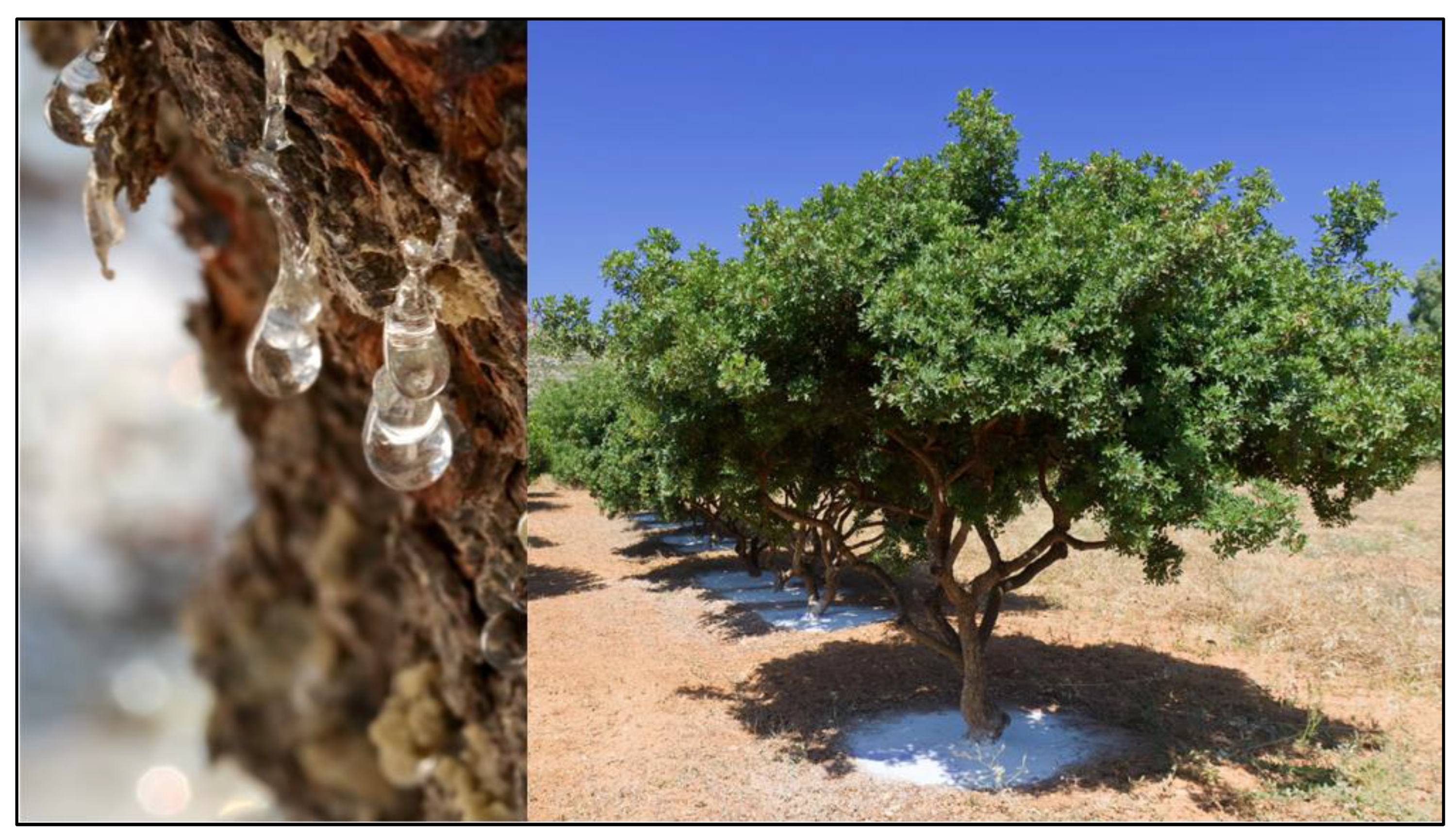
The cultivation is only accomplished in the south part of Chios, due to the dry and hot climate. Mastic trees are evergreen shrub with a height of 2–3 m (rarely up to 5) which are found in small flat areas, in valleys, along roadsides or near the villages (Figure 2). In mountainous areas where the ground has a relative slope, there are cultures in steps. In general, the mastic trees have few soil requirements and thrive in barren, rocky, and poor soil. The total cultivated area of mastic is 20 km², which represents approximately the 12% of the total cultivated area of the island. The 2 million mastic trees that are estimated to be in this area, are engaged with 4500 agricultural families and therefore are very important for the local economy.

The mastic trees live more than 100 years, but they provide resin from their 5th year until their 70th. The care of the mastic groves extends over the whole year, since they grow in summer, but during the winter months it is necessary to prune and thin the branches. Around June, the surrounding ground is cleaned of weeds and it is spread with sieved white soil. This avoids the resin dripping and drying into the brown soil or to darken. Then, between July and October, the harvesting of the resins takes place.

Though there are many varieties of mastic trees growing throughout the Mediterranean, it is only in the Greek island of Chios that the production of gum mastic occurs. There was no successful development elsewhere, in the continental or insular Greece or even in the neighboring coasts of Turkey. Within the European Union, mastic production in Chios is granted a protected designation of origin. Originally a liquid, mastic is sun-dried into drops of hard brittle translucent resin. When chewed, the resin softens and becomes a bright white and opaque gum. The flavor is bitter at first, but after some chewing, it releases a refreshing, slightly pine or cedar-like flavor. Mastic appears to have a myriad of applications ranging from the medicinal to the functional, including use as a stabilizer in paints and making varnishes, especially for musical instruments. It has been used in the production of tires, aromatic soaps, insecticides, electrical insulators, and chewing gum, as well as quality spices, alcoholic beverages, and sweets. The total annual production is 150 tn and 90% of the product is exported. With a price range of 180–250 EUR/kg, this exclusive product is considered as a major part of the local economy.

3.3. Local Reactions and Awareness

The local population of Chios was informed about the plans for the installation of the AIGAIA ZEUXI project on the North Aegean islands in 2006 followed by an initial intense reaction by the local communities. In March 2012, the Ministry of Environment, Energy and Climate Change set in public consultation the Environmental Impact Assessment for the creation of wind farms in the three islands of the North Aegean. The local society reacted directly, and a local organization named “Chios’ Citizens and Windmills” was set up. A public awareness campaign was initiated in parallel with documentation on the investment, the impacts, and the benefits for the local societies. A network of information and knowledge exchange was set up among the North Aegean Islands. This organization asked for the cancellation of the project presenting cultural, environmental sensitivity, and possible effects on the microclimate and especially on the mastic trees cultivation.

4. CFD Modelling

4.1. Governing Equations

The governing equations of the flow field solved by Fluent are the continuity and conservation of momentum equations [15]:

$$\frac{\partial \rho }{\partial t}+\nabla ·\left(\rho \overrightarrow{u}\right)=0$$

(1)

$$\frac{\partial }{\partial t}\left(\rho \overrightarrow{u}\right)+\nabla ·\left(\rho \overrightarrow{u}\overrightarrow{u}\right)=-\nabla p+\nabla ·\left(\stackrel{=}{\tau }\right)+\rho \overrightarrow{g}+S_M$$

(2)

In Equations (1) and (2), $\rho$ is the air density, $\overrightarrow{u}$ is the fluid velocity vector, $\overrightarrow{g}\mathrm{is}\mathrm{the}\mathrm{gravitational}\mathrm{acceleration},$ $p$ the pressure, $\stackrel{=}{\tau }$ the shear stress tensor, and $S_M$ a momentum source term. The stress tensor, is related to the strain rate as follows:

$$\stackrel{=}{\tau }=\mu \left[\nabla \overrightarrow{u}+\nabla {\overrightarrow{u}}^T-\frac{2}{3}·\nabla ·\overrightarrow{u}I\right]=0$$

(3)

where $\mu$ is the dynamic viscosity of the fluid, $\nabla \overrightarrow{u}$ denotes the velocity gradient, with $T$ denoting the transpose of the matrix, and $I$ is the unit tensor.

4.2. Turbulence Modelling

The turbulence modelling at the Reynolds-Averaged Navier–Stokes (RANS) approach requires the modeling and correlation of the Reynolds stresses to the mean velocity gradients. The Boussinesq hypothesis is used in the $k-\epsilon$ model using the following relation:

$$-\rho \overline{u_i^{\prime }{u}_j^{\prime }}={\mu }_t\left(\frac{\partial u_i}{\partial x_j}+\frac{\partial u_j}{\partial x_i}\right)-\frac{2}{3}\left(\rho k+{\mu }_t\frac{\partial u_k}{\partial x_k}\right){\delta }_{ij}$$

(4)

where ${\delta }_{ij}$ is the Kronecker’s delta, $k$ is the turbulence kinetic energy, and ${\mu }_t$ the turbulent viscosity.

The $k-\epsilon$ turbulence closure scheme was appropriately parameterized for atmospheric flows. It assumes ${\mu }_t$ is an isotropic scalar quantity and it is computed as a function of the model transport equations for the turbulence kinetic energy, $k$ and its dissipation rate, $\epsilon$. The two additional transport equations are given below [15]:

$$\frac{\partial \left(\rho k\right)}{\partial t}+\frac{\partial \left(\rho k{u}_i\right)}{\partial x_i}=\frac{\partial }{\partial x_j}\left[\left(\mu +\frac{{\mu }_t}{{\sigma }_k}\right)\frac{\partial k}{\partial x_j}\right]+G_k+G_b-\rho \epsilon -Y_m+S_k$$

(5)

$$\frac{\partial \left(\rho \epsilon \right)}{\partial t}+\frac{\partial \left(\rho \epsilon u_i\right)}{\partial x_i}=\frac{\partial }{\partial x_j}\left[\left(\mu +\frac{{\mu }_t}{{\sigma }_{\epsilon }}\right)\frac{\partial \epsilon }{\partial x_j}\right]+C_{1\epsilon }\frac{\epsilon }{k}\left(G_k+C_{3\epsilon }{G}_b\right)-C_{2\epsilon }\rho \frac{{\epsilon }^2}{k}+S_{\epsilon }$$

(6)

In Equations (5) and (6), $G_k$ represents the generation of turbulence kinetic energy $k$ due to the mean velocity gradients, $G_b$ is the generation rate of $k$ due to buoyancy, $Y_M$ is the contribution of the fluctuating dilatation in compressible turbulence to the overall dissipation rate, and $S_k$ and $S_{\epsilon }$ are source terms.

The turbulent (or eddy) viscosity, ${\mu }_t$ is computed by:

$${\mu }_t=\rho C_{\mu }\frac{k^2}{\epsilon }$$

(7)

where $C_{\mu }$ is a constant. The constants of the standard $k-\epsilon$ model are modified according to the analysis presented in detail in Prospathopoulos et al. [16] as follows:

$$C_{\mu }=0.033,\hspace{1em}{C}_{1\epsilon }=1.12,\hspace{1em}{C}_{2\epsilon }=1.83,\hspace{1em}{\sigma }_k=1.0,\hspace{1em}{\sigma }_{\epsilon }=1.3$$

(8)

4.3. Modelling of the Atmospheric Boundary Layer (ABL)

Stable atmospheric conditions are modelled by means of an additional buoyancy production (or dissipation) term $f·G_b$ which is added to the $k$ and $\epsilon$ equations, without solving an additional conservation equation for energy or temperature. This term takes the form:

$$G_b=-{\mu }_t{\left(\frac{\partial u}{\partial z}\right)}^2·\frac{Ri}{f_m}$$

(9)

$$Ri=\zeta \frac{0.74+4.7\zeta }{{\left(1+4.7\zeta \right)}^2}$$

(10)

$$f_m=1+5\zeta$$

(11)

$$\zeta =\frac{z}{L}$$

(12)

where ${\mu }_t$ is the turbulent viscosity, $Ri$ is the Richardson number, and $L$ the Monin-Obukhov length.

As adopted in [15], $f=1$ and $f=0$ for $k$ and $\epsilon$ equations, respectively (the additional term is added only to the $k$ equation).

The inlet conditions for wind velocity, $k$, and $\epsilon$ are given by the Monin–Obukhov similarity profiles for stable atmospheric stratification [17,18]:

$$u_0\left(z\right)=\frac{u_{*}}{\kappa }\left[\ln \left(\frac{z}{z_0}\right)+5\frac{z}{L}\right]$$

(13)

$$k_0\left(z\right)=\frac{u_{*}^2}{\sqrt{C_{\mu }}}·{\left(\frac{f_{\epsilon }}{f_m}\right)}^{0.5}$$

(14)

$${\epsilon }_0\left(z\right)=\frac{u_{*}^3}{\kappa ·z}·f_{\epsilon }{\left(\frac{f_{\epsilon }}{f_m}\right)}^{0.5}$$

(15)

where $f_{\epsilon }=1+4\frac{z}{L}$, $u_{*}$ is the friction velocity, $z$ is the vertical height, $z_0$ the roughness height, and $\kappa =0.41$, the von Karman’s constant.

The above profiles reduce to the well-known profiles for neutral atmospheric conditions [17,18,19,20] as the Monin–Obukhov length $L$ takes very large values (positive or negative).

4.4. Modelling of the Wind Turbines

The rotor disks are approximated as momentum sinks to represent the axial force $T$ across the disk, associated with a constant thrust coefficient $C_T$ over the rotor area:

$$T=0.5\rho U_{ref}^2{C}_{T}A$$

(16)

where $A$ is the surface area of the rotor disk and $\rho$ is the air density.

For the estimation of the thrust coefficient and the thrust force, a reference freestream wind speed $U_{ref}$ must be estimated. Once $U_{ref}$ is known, the thrust coefficient $C_T$ is estimated using the manufacturer-given thrust curve of the turbine, considered as uniform over the rotor disk. However, in real flow cases the flow and the thrust coefficient are not uniform over the rotor disk because of the atmospheric boundary layer shear and the finite number of rotating blades with varying span-wise properties. A non-uniform force over the rotor disk area $C_T$ would perhaps require coupling of the CFD solver with a Blade Element Momentum (BEM) theory solver. However, this option requires detailed data for the blade geometry and the $C_L$,$C_D$ curves of the airfoils along the span of the blades that are usually not available. Local effects produced by the radial variation of $C_T$ would result in a non-uniform near-wake profile expected to diminish at a distance of about one rotor diameter downstream. In all cases, a reference wind speed must be estimated.

In the case of a wind farm, a wind turbine may operate in the wake of one or more wind turbines. The accurate prediction of its power requires an accurate prediction of the wake effects from the upstream machines, which, in turn, involves the accurate estimation of the reference wind speed for the reliable estimation of the thrust coefficient. From the numerical modeling point of view, there is no obvious approach to estimate the thrust coefficient since the wind turbine power and thrust curves are usually provided for single-machine operation rather than operation in the wake of another wind turbine generator. Consequently, there is a deficiency in the definition of the appropriate wind speed used for the calculation of the wind turbine’s thrust force or power in wake operation [19,21,22,23,24].

In the current project a constant reference wind speed of 8 m/s has been used at the hub height at the inlet plane. The reason for simulating this wind speed is to simulate the worst-case scenario. Based on preliminary tests, at a lower speed the total deficit of the velocity downstream was smaller and higher speeds were reducing wake propagation due to higher atmospheric turbulence and thus entrainment. Obtained wake results and the flow behavior downstream are in accordance with other numerical and experimental investigations using Actuator Disk Model (ADM) in different ambient turbulence and inflow conditions [19,23,24,25,26,27,28,29,30].

4.5. Computational Domain and Wind Farm Positioning

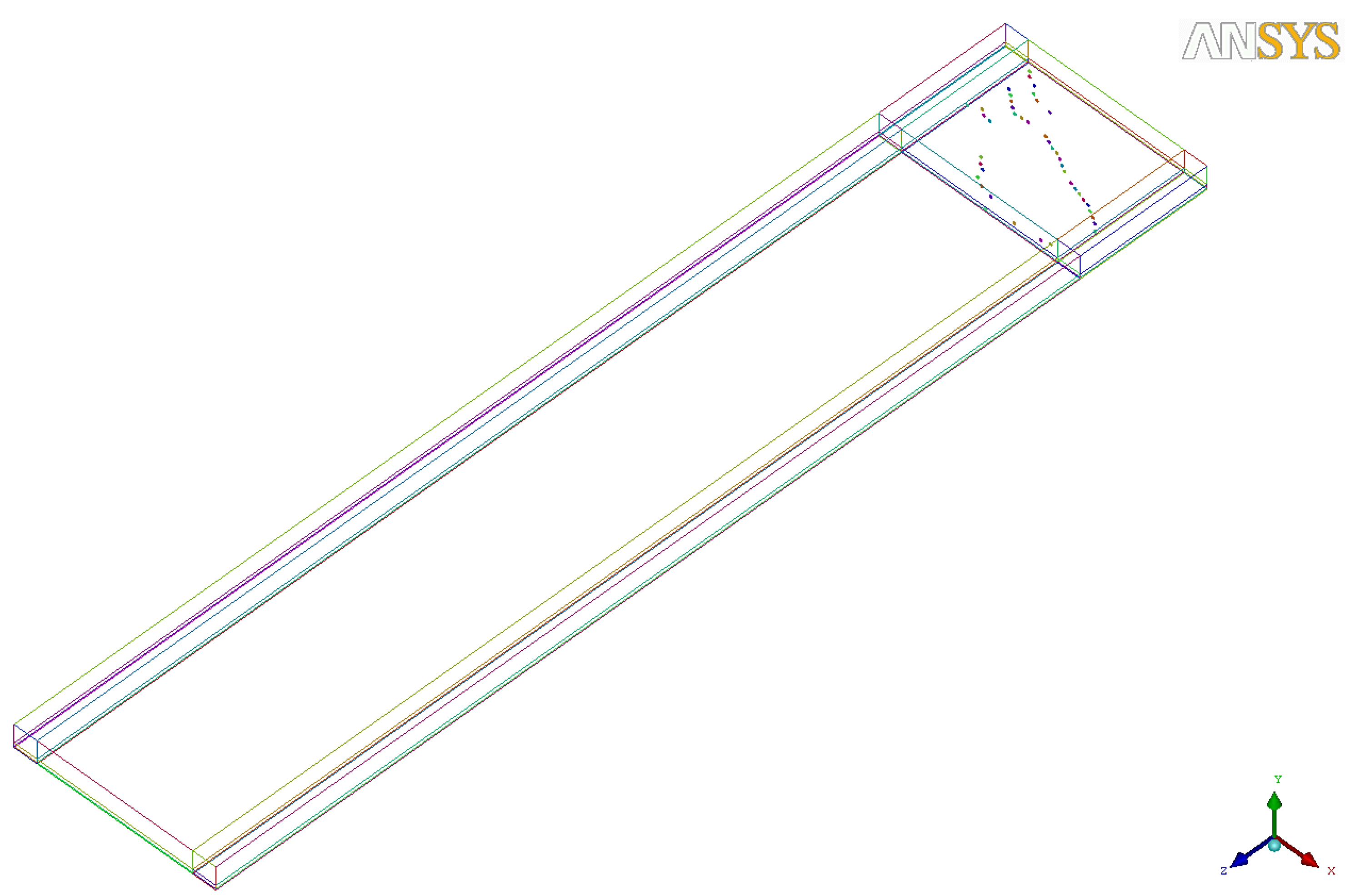
The analysis is carried out with the use of the commercial CFD code ANSYS Fluent [31]. The size of the computational domain is $7\mathrm{km}$ wide, $800\mathrm{m}$ height, and $34.4\mathrm{km}$ long (Figure 3). The computational grid is a multi-block mesh of approximately $14\mathrm{M}$ hexahedral elements which was created in ANSYS ICEM software package. The area of interest that includes all the wind farms, has been well refined with uniform cubic elements of $4^3{\mathrm{m}}^3$ (Figure 4d). This area has been extended at a distance of five rotor diameters upstream of the first wind turbine to let the incoming flow develop. It starts at a height of $40\mathrm{m}$ up to a height of $160\mathrm{m}$ assuming $80\mathrm{m}$-diameter wind turbines and hub heights at $80\mathrm{m}$ above the ground. At the blocks of the bottom (covering the height from ground to $40\mathrm{m}$), as well as at the blocks of the upper part of the domain (from $160\mathrm{m}$ to $800\mathrm{m}$), an exponential function has been used with a ratio $R=1.10.$ As a result the first cell height at the ground was 0.5 m. Downstream the area of interest a similar exponential function with ratio $R=1.10$ was also used.

The internal cells that were chosen to model the wind turbines, represent the total size of the $80\mathrm{m}$ rotor diameters and were located according to the project layout and positioning of the wind farms (Figure 4d). The first wind farm that was located at the northern part of the island was not included since it was located 4 km away from the current arrays and approximately 20 km away from the south part of the island where the mastic trees under investigation were located.

To extract the wind farms positioning, the initial map of the project has been projected on the Google maps [32] (Figure 4a,b). The final coordinates of the wind turbines were extracted as points, transformed to Cartesian coordinates, and used for the selection of the internal cells (Figure 4c,d).

4.6. Numerical Setup, Initital and Boundary Conditions

For the solution the Semi-Implicit Method for Pressure Linked Equations (SIMPLE) solver of ANSYS Fluent was used to solve the three-dimensional, incompressible, steady state Reynolds Average Navier–Stokes (RANS) using second order numerical schemes and the QUICK (Quadratic Upstream Interpolation for Convective Kinematics) higher-order differencing scheme that considers a three-point upstream weighted quadratic interpolation for the cell face values. As described above, the computational domain was structured with hexahedral elements that were aligned with the flow and refined at the area of interest to improve the accuracy [15]. Boundary conditions are given at

Table 1. Boundary conditions.

Inlet	User Defined Functions (UDF) for $u_0\left(z\right)$, $k_0\left(z\right)$ and ${\epsilon }_0\left(z\right)$.
Outlet	Pressure outlet, using zero fixed value.
Bottom	Wall function with constant roughness.
Sides and Top	Symmetry conditions.

.

Two simulations with different turbulence intensities were conducted, $TI=8\%$ and $TI=15\%$, as described in Section 1. The initial values and the boundary conditions for the turbulence quantities have been calculated separately for each case according to the $TI$ and were introduced with user defined functions using the set of equations presented in Section 4.2 and 4.3. Atmospheric air was chosen as fluid, with constant density $\rho =1.225\mathrm{kg}/{\mathrm{m}}^3$ and dynamic viscosity $\mu =1.225\mathrm{kg}/{\mathrm{m}}^3$. A positive value of 365 m has been used for the Monin–Obukhov length ($L$) to model a stable atmospheric stratification. A reference speed of $U_{ref}=8\mathrm{m}/\mathrm{s}$ at HUB height $H_{ref}=80\mathrm{m}$ has been used in both cases.

5. Results and Discussion

Different mesh refinements have been tested at the rotor-wake region with actuator disk rotors and the k-ε turbulence model to achieve a mesh independent solution. In all cases, results at the far wake regions (>15 diameters) were not affected from local refinements at the wind farms area upstream. Solutions converged with residuals below ${10}^{-4}$ for pressure and below ${10}^{-6}$ for the turbulence parameters and the three velocity vectors.

At the following pages results of the turbulence kinetic energy (TKE) and velocity deficits for the two cases of $TI=8\%$ (Figure 5a and Figure 6, Figure 8a and Figure 9a) and $TI=15\%$ (Figure 5b, Figure 7, Figure 8b and Figure 9b) are presented.

The TKE production k is compared against the expected ambient TKE production at the hub heights for the two cases using the following equation:

$$k=\frac{3}{2}{\left(TI{U}_{ref}\right)}^2$$

(17)

where $U_{ref}$ the reference velocity at hub height $H_{ref}$.

The flat terrain that was chosen for the simulations diminish any additional turbulence effects of the ground at that height and benefits the wake propagation. As already mentioned above, this case aims to simulate the worst-case scenario and therefore overestimate the wake effects. By taking into account the island topography the wake effects, which express the wind farms impact to the local flow field, would be negligible. In complex terrains, with high ambient turbulence, the multiple wakes would recover faster, and any potential impact would be eliminated in a shorter distance.

For the case of $TI=8\%$ (Figure 5) the wake effects are observed at a maximum distance of 5 km, whereas for $TI=15\%$ (Figure 6), they have already been eliminated at the same distance. The slices of Figure 5 and Figure 6 show the additional turbulence that was produced by the wind farms. In order to qualitative compare the results, in Figure 5 and Figure 9 the TKE and velocity deficit, respectively, are projected for both cases on the complex terrain of Chios using Google Earth [33].

Following the trend of turbulence kinetic energy, the velocity deficit that was observed for the case of low turbulence intensity $TI=8\%$ (Figure 8a and Figure 9a), was greater against the case of $TI=15\%$ (Figure 8b and Figure 9b). Additionally, results confirm that in higher ambient turbulence conditions, the wake recovery is faster. This occurs from the increased mixing of the wake effects with the ambient free stream flow. For the same reason, a faster wake recovery takes place also in higher wind speeds (>8$\mathrm{m}/\mathrm{s}$). Therefore, the choice of a reference wind speed $U_{ref}=8\mathrm{m}/\mathrm{s},$ with the current wind turbine modelling characteristics, helps the wake propagation further downstream.

By investigating the velocity deficit and the turbulence kinetic energy downstream the wind farms it is clear that for the current layout, any impact will be eliminated after 10 rotor diameters downstream, even at the non-realistic worst-case scenario of low turbulence intensity. Figure 5 and Figure 9 aim also to present the local complexity and increased roughness of the ground which in practice is expected to increase the vertical mixing of the flow and therefore reduce further the wake effects downstream.

6. Lessons Learnt—Conclusions

The physical problem of flow over wind farms and their impact on the Chios microclimate for the large-scale project “Aigaia Zeufxi” is addressed. Two cases with different turbulent intensities, $TI=8\%$ and $TI=15\%$ are explored. Simulations were performed with steady state solutions of the incompressible RANS using a stable atmospheric stratification and user defined functions at the commercial CFD solver ANSYS Fluent. Wind turbines were modeled as momentum sinks with uniform loaded actuator disk models. The velocity deficit and the increased turbulent levels that were observed are in line with the current literature and other investigations on wind turbine wake effects [16,19,21,22,23,24,25,26,27,28,29,30].

The propagation of the multiple wake effects is reduced with the distance downstream and according to Figure 5, slice CC’ at the plane-yz and for x = 10 km, it is already eliminated at a distance of 10 km for the worst-case scenario with $TI=8\%$. This value of turbulence intensity is usually observed in flows over sea in offshore applications. For the more realistic case of $TI=15\%$, according to the complex terrain of Chios island, the wake effects are eliminated 5 km downstream.

Considering the relation of turbulence production with the turbulence intensity (Equation (17)) and the ABL stratification, there will be no impact on the microclimate related to the operation of the wind turbines under investigation after 10 km downstream.

For the case of Chios, “Mastichochoria” are located in a distance of more than 15 km downstream from the last southern wind turbine. By taking into consideration the complex terrain of Chios, the altitude difference between “Mastichochoria” and the project area under investigation, we can clearly declare that the wind turbines will not affect the mastic trees.

To conclude, the current research improvises that for wind farms of relevant and smaller size, there is not obvious disturbance of the microclimate beyond a distance of 8 km (100 rotor diameters). For this particular case, the local authorities should worry more for the impact of the upcoming greenhouse effect rather than the deployment of wind farms at the northern part of the island. Nevertheless, wind energy community should be further motivated to investigate the “green-development” of the wind energy sector by taking into account and consideration any possible local environmental and economic impacts and therefore ensure the long-term sustainability of the sector. Further steps should be also done to educate the local communities and the new generations about the benefits and the necessity to a transition towards green energy.

Last but not least, special care should be given at the layout of wind farms since wake effects are of great importance for the long-term sustainability of a project. Increased turbulence results to fatigue of materials and therefore unexpected corrective maintenance expenses for failures of the installed equipment. Additionally, wake effects are characterized by reduced wind speeds downstream, which affect the total power production. Results with small turbulence intensity indicate that there should be an extra care given in offshore applications where wake effects and effects of neighboring wind farms are more dominant. Each case should be considered unique and analyzed individually, taking into consideration the wind farm design, local and surrounding topography, climate, land use, and local activities.

References

- Regulatory Authority of Energy (RAE). Methodology for the Assessment of Wind Penetration in Non-Interconnected Islands. 2003. Available online: http://www.rae.gr/K2/deliberation-ape.html (accessed on 26 December 2012).
- Caralis, G.; Zervos, A. Analysis of wind power penetration in autonomous greek Islands. Wind. Eng. 2007, 31, 487–502. [Google Scholar] [CrossRef]
- Hellenic Transmission System Operator. Study for the Interconnection of Aegean Islands with the Mainland, Athens. 2010. Available online: http://www.desmie.gr/fileadmin/user_upload/Files/Consultations/AIGEA_INTERCONNECTION_PHASE_A.pdf (accessed on 26 December 2012).
- Papadopoulos, E.K.M.; Papathanassiou, S.; Tsili, M. Interconnection Strategy of Islands to the Mainland Grid, Athens. 2006. Available online: http://www.rae.gr/cases/C19 (accessed on 26 December 2012).
- Georgiou, P.N.; Mavrotas, G.; Diakoulaki, D. The effect of islands’ interconnection to the mainland system on the development of renewable energy sources in the Greek power sector. Renew. Sustain. Energy Rev. 2011, 15, 2607–2620. [Google Scholar] [CrossRef]
- Roy, S.B. Simulating impacts of wind farms on local hydrometeorology. J. Wind Eng. Ind. Aerodyn. 2011. [Google Scholar] [CrossRef]
- Roy, S.B.; Traiteur, J.J. Impacts of wind farms on surface air temperatures. Proc. Natl. Acad. Sci. USA 2010, 107, 17899–17904. [Google Scholar]
- Roy, S.B.; Pacala, S.W.; Walko, R.L. Can large wind farms affect local meteorology? J. Geophys. Res. 2004, 109, D19101. [Google Scholar] [CrossRef]
- Adams, A.S.; Keith, D.W. Wind energy and climate: Modeling the atmospheric impacts of wind energy turbines. In EOS Trans AGU 88 Fall Meeting Supplement; American Geophysical Union: Washington, DC, USA, 2007. [Google Scholar]
- Zhou, L.; Tian, Y.; Roy, S.B.; Thorncroft, C.; Bosart, L.F.; Hu, Y. Impacts of wind farms on land surface temperature. Nat. Clim. Chang. 2012, 2, 539–543. [Google Scholar] [CrossRef]
- Armstrong, A.; Waldron, S.; Whitaker, J.; Ostle, N.J. Wind farm and solar park effects on plant–soil carbon cycling: Uncertain impacts of changes in ground-level microclimate. Glob. Chang. Biol. 2014, 20, 1699–1706. [Google Scholar] [CrossRef]
- Cervarich, M.C.; Roy, S.B.; Zhou, L. Spatiotemporal Structure of Wind Farm-atmospheric Boundary Layer Interactions. Energy Procedia 2013, 40, 530–536. [Google Scholar] [CrossRef] [Green Version]
- Chamorro, L.P.; Porté-agel, F. Effects of Thermal Stability and Incoming Boundary-Layer Flow Characteristics on Wind-Turbine Wakes: A Wind-Tunnel Study. Bound.-Layer Meteorol. 2010, 515–533. [Google Scholar] [CrossRef] [Green Version]
- Hellenic Statistical Authority. Greece in Figures January–March 2021. Available online: http://dlib.statistics.gr/Book/GRESYE_01_0005_00002.pdf (accessed on 1 April 2021).
- ANSYS Fluent Theory Guide; ANSYS Inc.: Canonsburg, PA, USA, 2013.
- Prospathopoulos, J.M.; Politis, E.S.; Rados, K.G.; Chaviaropoulos, P.K. Evaluation of the effects of turbulence model enhancements on wind turbine wake predictions. Wind. Energy 2010, 14, 285–300. [Google Scholar] [CrossRef]
- Stull, R.B. An Introduction to Atmospheric Boundary Layer Meteorology, 1st ed.; Springer: Amsterdam, The Netherlands, 1988. [Google Scholar] [CrossRef]
- Panofsky, H.; Dutton, J. Atmospheric Turbulence; Wiley: New York, NY, USA, 1984. [Google Scholar]
- Rados, K.; Mosfilis, S.; Stergiannis, N.; Tourlidakis, A.; Caralis, G.; Zervos, A. CFD modeling approaches of wind turbine single and multiple wakes. In Proceedings of the 2012 European Wind Energy Conference & Exhibition, Copenhagen, Denmark, 19 April 2012; pp. 1842–1849. [Google Scholar]
- Blocken, B.; van der Hout, A.; Dekker, J.; Weiler, O. CFD simulation of wind flow over natural complex terrain: Case study with validation by field measurements for Ria de Ferrol, Galicia, Spain. J. Wind. Eng. Ind. Aerodyn. 2015, 147, 43–57. [Google Scholar] [CrossRef]
- Prospathopoulos, J.M.; Politis, E.S.; Chaviaropoulos, P.K. Modelling Wind Turbine Wakes in Complex Terrain. In Proceedings of the European Wind Energy Conference, EWEC, Brussels, Belgium, 31 March–3 April 2008. [Google Scholar]
- Vermeer, L.J.; Sørensen, J.N.; Crespo, A. Wind turbine wake aerodynamics. Prog. Aerosp. Sci. 2003, 39, 467–510. [Google Scholar] [CrossRef]
- Barthelmie, R.J.; Rathmann, O.; Frandsen, S.T.; Hansen, K.S.; Politis, E.; Prospathopoulos, J.; Rados, K.; Cabezón, D.; Schlez, W.; Phillips, J.; et al. Modelling and measurements of wakes in large wind farms. J. Phys. Conf. Ser. 2007, 75, 012049. [Google Scholar] [CrossRef]
- Barthelmie, R.J.; Hansen, K.; Frandsen, S.T.; Rathmann, O.; Schepers, J.G.; Schlez, W.; Phillips, J.; Rados, K.; Zervos, A.; Politis, E.S.; et al. Modelling and measuring flow and wind turbine wakes in large wind farms offshore. Wind. Energy 2009, 12, 431–444. [Google Scholar] [CrossRef]
- Vafiadis, K.; Stergiannis, N.; Tourlidakis, A.; Rados, K.G. Computational investigation of horizontal axis wind turbine wake. In Proceedings of the European Wind Energy Conference & Exhibition, 2013, EWEC, Vienna, Austria, 4–7 February 2013; pp. 1692–1700. [Google Scholar]
- Stergiannis, N.; Rados, K.G.; Caralis, G.; Lacor, C.; Donnelly, R.; Tourlidakis, A.; Perivolaris, I.; Zervos, A. CFD modelling approaches of onshore wind farms and their potential impact on the microclimate of Chios. In Proceedings of the European Wind Energy Conference & Exhibition, 2014, EWEA, Barcelona, Spain, 10 March 2014. [Google Scholar]
- Stergiannis, N.; van Beeck, J.; Runacres, M.C. Full HAWT rotor CFD simulations using different RANS turbulence models compared with actuator disk and experimental measurements. Wind Energ. Sci. Discuss. 2017. preprint. [Google Scholar] [CrossRef]
- Sørensen, J.; Shen, W.Z.; Munduate, X. Analysis of Wake States by a Full-Field Actuator Disc Model. Wind Energy 1998, 1, 73–88. [Google Scholar] [CrossRef]
- Troldborg, N.; Sorensen, J.N.; Mikkelsen, R. Numerical simulations of wake characteristics of a wind turbine in uniform inflow. Wind. Energy 2010, 13, 86–99. [Google Scholar] [CrossRef]
- Magnusson, M. Near-wake behaviour of wind turbines. J. Wind. Eng. Ind. Aerodyn. 1999, 80, 147–167. [Google Scholar] [CrossRef]
- ANSYS, Fluent. Available online: http://www.ansys.com/Products/Fluids/ANSYS-Fluent (accessed on 1 April 2021).
- Google. (n.d.). Chios, Greece. Available online: https://goo.gl/maps/HSJ4eSoey9zVZ6Pd8 (accessed on 1 April 2021).
- Google Earth v7.0. (8 September 2006). Chios, Greece. 38°22′05′′ N, 26°05′05′′ E, Eye alt 130 km. DigitalGlobe 2012. Available online: http://www.earth.google.com (accessed on 1 April 2021).