Article

Fully Implicit Stress Update Algorithm for Distortion-Based Anisotropic Hardening with Cross-Loading Effect: Comparative Algorithmic Study and Application to Large-Size Forming Problem

1
Department of Materials Science and Engineering & RIAM, Seoul National University, Seoul 08826, Korea
2
Steel Solution Research Lab, POSCO, 100 Songdogwahak-ro, Yeonsu-gu, Incheon 21985, Korea
*
Author to whom correspondence should be addressed.
These authors contributed equally to this work.
Submission received: 20 May 2021 / Revised: 6 June 2021 / Accepted: 8 June 2021 / Published: 14 June 2021
(This article belongs to the Special Issue Advanced Structure Materials and Processing)

Abstract

:
A fully implicit stress integration algorithm is developed for the distortional hardening model, namely the e-HAH model, capable of simulating cross-hardening/softening under orthogonal loading path changes. The implicit algorithm solves a complete set of residuals as nonlinear functions of stress, a microstructure deviator, and plastic state variables of the constitutive model, and provides a consistent tangent modulus. The number of residuals is set to be 20 or 14 for the continuum or shell elements, respectively. Comprehensive comparison programs are presented regarding the predictive accuracy and stability with different numerical algorithms, strain increments, material properties, and loading conditions. The flow stress and r-value evolutions under reverse/cross-loading conditions prove that the algorithm is robust and accurate, even with large strain increments. By contrast, the cutting-plane method and partially implicit Euler backward method, which are characterized by a reduced number of residuals, result in unstable responses under abrupt loading path changes. Finally, the algorithm is implemented into the finite element modeling of large-size, S-rail forming and the springback for two automotive steel sheets, which is often solved by a hybrid dynamic explicit-implicit scheme. The fully implicit algorithm performs well for the whole simulation with the solely static implicit scheme.

1. Introduction

Automotive, non-ferrous alloys and advanced high-strength steels have been extensively investigated by many researchers owing to their lightweight and excellent mechanical properties. Lightweight alloys, such as aluminum and magnesium alloys, exhibit superior specific strengths to conventional steels. By contrast, the increased strength, which can exceed 1 GPa, enables the advanced high-strength steel (AHSS) sheets to have a thinner gauge, thus, rendering them more competitive compared to low-density, lightweight alloys. The excellent strength and enhanced ductility of the AHSS can be achieved owing to their well-controlled microstructure and deformation mechanisms. For example, dual-phase steels or transformation induced steels introduce a hard martensite phase embedded in the softer ferrite phase or transforming martensite from meta-stable austenite. The strength of lightweight alloys can be achieved through the dispersion of optimally designed second phases, such as precipitations.
However, even in the presence of these improved plasticity properties, such as tensile strength and elongation at fracture, the intricate microstructure leads to a further complexity in the mechanical properties, especially when the deformation paths become convoluted. The complex mechanical responses include the Bauschinger effect and transient flow behavior under reversed loading path [1,2,3,4,5]. These anisotropic hardening behaviors of sheet metals have been reported to be critical factors for the springback of automotive sheet parts [6,7,8,9]. More recently, the anisotropic hardening behavior of advanced sheet metals has been further investigated under more complex loading paths than simple reverse loading. For instance, the deformation of ferritic-phased steels shows significant stress overshooting (or larger stress than the monotonic flow stress) when the loading path changes to being orthogonal to the previous loading path [10,11,12,13,14,15]. Interestingly, dual-phase steels with mixed ferrite and martensite phases exhibit a clear softening under the same loading path changes [15,16,17,18]. These plastic behaviors under orthogonal loading path changes are called cross-hardening and cross-softening, respectively. Experimental observations on these complex mechanical behaviors, which cannot be explained through the simple isotropic plasticity model, require the implementation of new anisotropic models in the field of metal forming and plasticity. Indeed, this complex behavior can influence the formability and springback of advanced sheet metals [9].
In the literature, a significant number of works have proposed models for anisotropic hardening behavior. Kinematic hardening is a representative concept, which explains the Bauschinger effect and transient flow hardening at load reversal by introducing yield surface translation during plastic deformation. The kinematic hardening models were pioneered by Prager [19] and Ziegler [20], and further extended by adding nonlinear terms [21] or by coupling with the isotropic hardening model. The series of isotropic and kinematic hardening models was well implemented into finite element (FE) simulations for sheet metals, especially when metals exhibit the Bauschinger effect, transient behavior, and permanent softening under reversed loading paths [22,23,24,25].
The kinematic hardening—based anisotropic hardening models were further extended by combing the distortional hardening concept to reproduce mechanical responses under rather complex loading conditions, beyond the simple loading-reverse loading path. Ortiz and Popov [26] introduced the distortion of the yield surface by controlling the size of the effective stress. Feigenbaum and Dafalias [27,28] employed the fourth-rank anisotropic tensor as a function of plastic deformation, but the fundamental basis they used remained that of isotropic-kinematic hardening. Teodosiu and Hu [29] introduced new effective values into the yield condition related to the structure and interactions of dislocations as a major plasticity mechanism. François [30] expressed the egg-shaped yield function by decomposing deviatoric stress into its collinear and orthogonal parts with respect to the back stress of kinematic hardening. Badreddine et al. [31] developed a non-associated elastoplastic anisotropic hardening model, which is coupled with a damage model based on François’s approach [30]. Qin et al. [32] suggested a model to represent the Bauschinger effect with the kinematic hardening component, while other strain-path change effects could be expressed through the distortion of the yield surface.
Besides the kinematic hardening or combined kinematic-distortional hardening, several anisotropic hardening models are solely based on the distortional hardening approach. Some of the distortional hardening models were developed to express the yield surface evolution by using the anisotropic coefficients as a function of the plastic work or equivalent plastic strain [33,34,35,36]. However, these models do not take into account the loading path change effect. Barlat and one the of co-authors of the present study [37,38,39] proposed a series of anisotropic hardening models without yield surface translation, which they named the homogeneous yield function based anisotropic hardening (HAH) models. The main concept of the original HAH model consists of using the distortion of the yield surface along a designated loading path, which is called a microstructure deviator, and the distortional amounts are controlled via adequately defined plastic state variables. Later, the model was extended for reproducing latent hardening, work hardening stagnation [38], as well as cross-hardening and softening under more general loading conditions [39]. This improved model was named the extended HAH model (or e-HAH, in this study). The performance of the distortional hardening models was validated through many applications, including the springback in U-draw bending and industrial S-rail forming [40,41,42,43,44,45,46]. The model is also applicable to subjects for which non-linear strain path effects are important, such as the fracture behaviors of metal after pre-deformation [47,48,49].
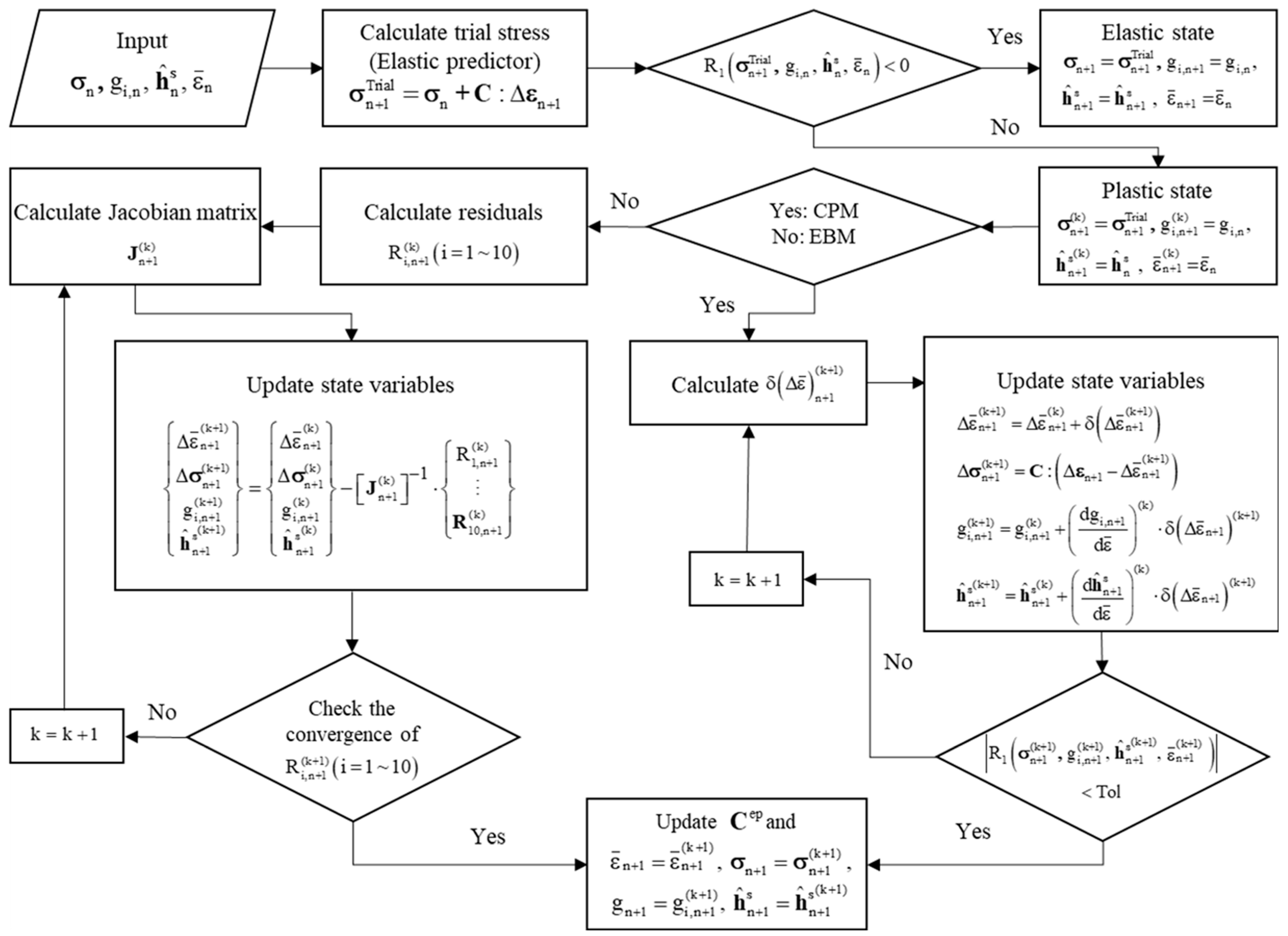
As the constitutive models of plasticity have advanced, especially the hardening laws, their implementation into FE simulations have become increasingly challenging. This is mainly attributed to the advanced constitutive models having more state variables, which are non-linearly cross-related. These challenges have led to more robust numerical formulations and implementations of the constitutive models, which eventually determine the accuracy and robustness of FE simulations. Numerous numerical algorithms were proposed to take into account the stress integration or stress update, using the elastic-plasticity constitutive models. The details of the general theoretical studies on these stress-integration algorithms for nonlinear plasticity are well documented in a book by Simo [50].
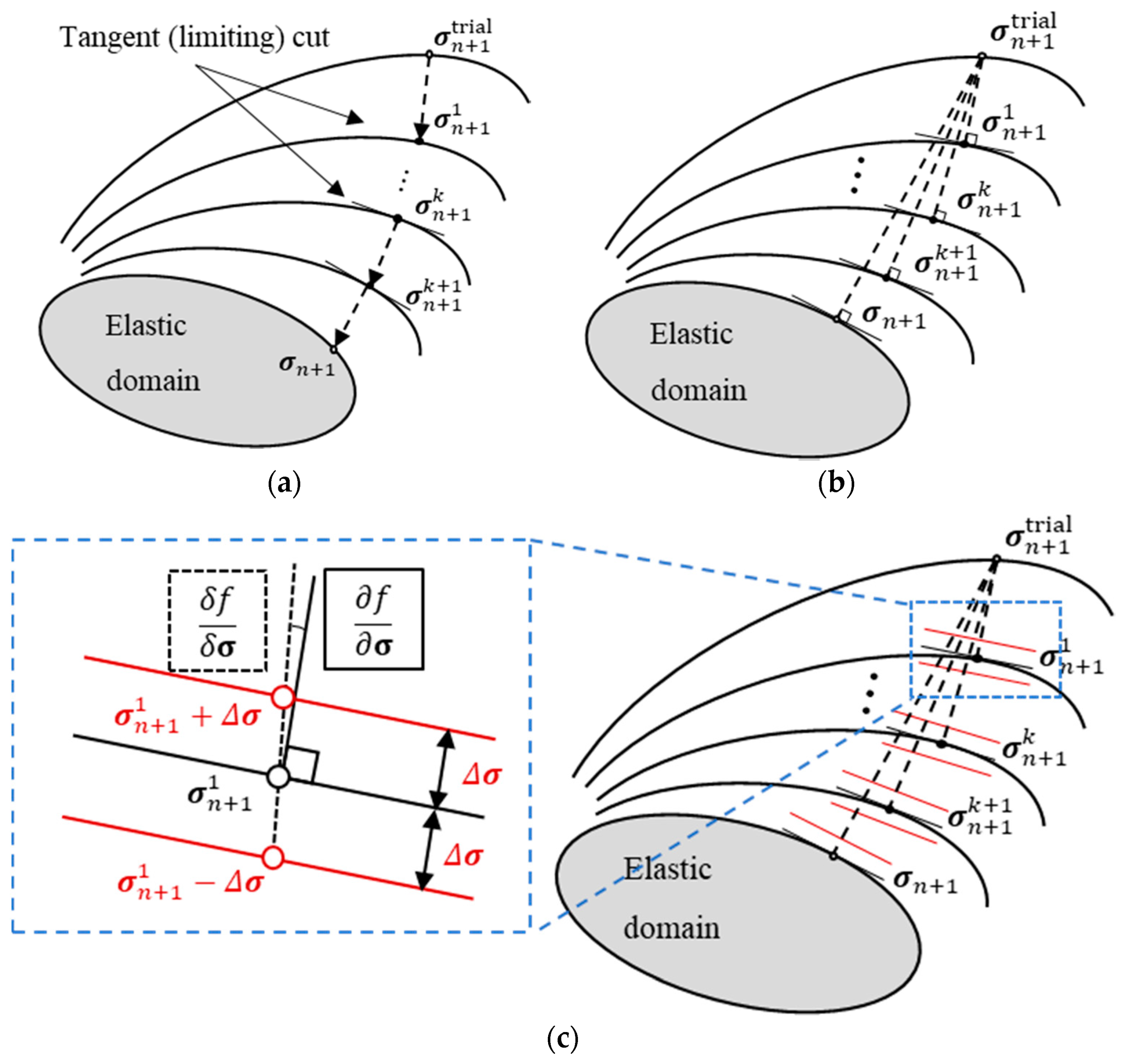
The basic principle of the stress update algorithm for the classical rate-independent elastoplastic model consists of locating the stress state on the yield surface described in the six-dimensional stress space, which is consistent with the material hardening. The hardening of the material is often represented by a uniaxial stress-plastic-strain curve as a reference stress state. Most of the stress update algorithms were developed in the elastic-predictor and plastic-corrector schemes. For example, the closest point projection method (CPPM) [51,52,53] and the cutting-plane method (CPM) [54] are employed as popular stress integration algorithms in FE models. The CPPM is often based on the Euler backward method (EBM), and thus it is an implicit method requiring the first and second derivatives of the yield surface to satisfy both the consistency and flow rule (or normality rule). In contrast, the CPM only satisfies the consistency condition without requiring the second derivative of the yield function; thus, this approach is also referred to as a semi-explicit method.
Regarding the stress integration algorithms on the distortional hardening models, similar approaches, based on either the CPPM or CPM schemes, have been reported. Lee et al. [55] implemented the first version of the HAH (denoted as original HAH hereafter) model into commercial ABAQUS software, using both the CPPM and CPM approaches. This implementation was also extended to the e-HAH model; however, in this case, only the CPM scheme was applied in combination with a sub-stepping numerical method [56]. Recently, Choi and Yoon [57] also reported the implementation of the HAH model, using the Euler backward scheme, but they calculated the derivatives of the yield function using numerical finite differences. More recently, Yoon et al. [58] coupled the CPPM scheme with a line-search algorithm for an updated version of the HAH model [59] to improve numerical efficiency. However, the existing numerical integration schemes do not fully exploit the implicit CPPM scheme. In other words, these approaches only account for the partial number of residuals in order to attain the solution process of linearized equations under the Newton-Raphson method. In this sense, these methods can be regarded as a partial or semi-implicit integration algorithm based on the Euler backward scheme.
In this study, a fully implicit stress integration algorithm based on the Euler backward scheme is proposed for the e-HAH model. To the best of our knowledge, the present work is the first to report this novel scheme. The present algorithmic study differs from previous studies [55,56,57,58] in that the complete set of residuals is established from the stress tensor, microstructure deviator, and other variables controlling the distortion of the yield function. Furthermore, the calculations of the first and second derivatives of the distorting yield function are both analytically expressed. Note that the CPPM or Euler backward scheme presented in previous studies adopted only the consistency condition and flow rule for the residuals. This may lead to non-physical evolutions of the distortional hardening state variables when there is an abrupt change in the loading path. For the comparative study on the effect of the employed stress integration algorithms, four different algorithms were implemented into the FE simulation. These algorithms consist of the CPM and EBM schemes with different numbers of residuals. Again, the EBM scheme is further classified based on either analytical derivatives or finite-difference—based numerical derivatives of the yield function. Comprehensive validations are presented in this study. Firstly, one-element analyses with two different material sets are presented for the investigated stress integration algorithms. The flow stress and anisotropy in deformation were evaluated under two distinctive loading conditions, i.e., reverse and cross-loading paths. Finally, the industrial-size S-rail forming and springback simulations were performed to evaluate the numerical accuracy and computational efficiency of the proposed algorithm. Note that even this large-scale industrial problem was solved using the purely static implicit FE solver, whereas most previous studies employed a dynamic explicit method for the forming process and a static implicit method for the springback, due to the divergence problem resulted from complex contact changes during forming.
The manuscript is organized as follows. In Section 2, a summary of the e-HAH model is presented. In Section 3, the numerical integration algorithms investigated in this study are introduced, alongside a summary of previous studies. Then, in Section 4, the accuracy and stability of the individual algorithms are comparatively evaluated via one-element analyses under two distinctive loading path changes. Finally, a large-scale industrial automotive forming and springback simulation is provided as a benchmark problem to assess the validity of the proposed, fully implicit numerical algorithm.

2. The e-HAH Model

The enhanced homogeneous yield function based anisotropic hardening (e-HAH) model was proposed to simulate the path-dependent anisotropic hardening responses of metallic materials. This model is based on the distortional hardening concept, without depending on kinematic hardening, and is capable of reproducing complex flow behaviors, such as cross-hardening or cross-softening [37,38,39].
The distortion of the initially isotropic yield function is controlled by a second-order tensor and eight scalar variables. The second-order tensor, named the microstructure deviator, h ^ s monitors the loading path changes and determines the direction of the distortion. The scalar variables control the magnitude of the distortions in terms of the loading path changes. In this section, the main equations of the constitutive model, along with the related evolution of the state variables, are briefly summarized. The complete derivations of the constitutive model can be found in [37,38,39].
The yield surface ( Φ ) of the e-HAH model is described as the following:
Φ = { ( ψ ( s ) 2 + ψ ( s P ) 2 ) q + f 1 q | h ^ s : s | h ^ s : s | | q + f 2 q | h ^ s : s + | h ^ s : s | | q } 1 / q = σ ¯
where σ ¯ is the equivalent stress, often identified from the uniaxial stress-plastic-strain curve as a reference state, and q is a constant. The two variables f i = ( g i q 1 ) q with i = 1 , 2 control the distortion of the yield surface along the direction of h ^ s . At the start of the simulation, h ^ s is initialized as h ^ i n i s = s i n i H s i n i : s i n i . Here, s i n i is the deviatoric stress corresponding to the initiation of the plastic deformation, and H is a constant, which is set to 8/3 in this work.
In Equation (1), ψ ( s ) 2 + ψ ( s P ) 2 represents the distorted yield function, which is used to reproduce the cross-hardening or softening; in the original HAH model, it is replaced by any first-order homogeneous yield function ϕ [37]. ψ ( s ) and ψ ( s P ) are defined in Equations (2) and (3), respectively, using the collinear ( s c ) and orthogonal ( s o ) components of the deviatoric stress tensor ( s ) with respect to h ^ s .
ψ ( s ) = ϕ ( s ) = ϕ ( s c + 1 g L s o ) ,
ψ ( s p ) = ϕ ( s p ) = ϕ ( 4 ( 1 g s ) g L s o ) ,
where s = s c + 1 g L s o and s p = 4 ( 1 g s ) s o are the two tensors, and g L and g S are the two corresponding state variables. The tensors s and s p are used for controlling the cross-hardening and softening, respectively. The two components are expressed as follows:
s c = H ( h ^ s : s ) h ^ s ,
s o = s s c = s H ( h ^ s : s ) h ^ s ,
To measure the loading path change, the indicator cos χ is introduced according to the following:
cos χ = h ^ s : s ^ h ^ s : h ^ s s ^ : s ^ = H ( h ^ s : s ^ ) ,
where the normalized deviatoric stress tensor is defined as s ^ = s H s : s . The value of cos χ indicates the current loading state against the previous loading path. For example, values of 1, 0, and −1 denote monotonic loading, cross-loading, and reverse loading, respectively.
The evolution laws for the state variables are summarized in three groups. The first group (Equations (7)–(10)) is related to the distortion along h ^ s :
d g 1 d ε ¯ = u 0 k 2 ( k 3 σ ¯ ( 0 ) σ ¯ ( ε ¯ ) g 1 ) + ( 1 u 0 ) k 1 g 4 g 1 g 1 ,
d g 2 d ε ¯ = u 0 k 1 g 3 g 2 g 2 + ( 1 u 0 ) k 2 ( k 3 σ ¯ ( 0 ) σ ¯ ( ε ¯ ) g 2 ) ,
d g 3 d ε ¯ = ( 1 u 0 ) k 5 ( k 4 g 3 ) ,
d g 4 d ε ¯ = u 0 k 5 ( k 4 g 4 ) ,
Here, u 0 is a unit step function with respect to cos χ . In other words, u 0 = 1 when cos χ 0 and u 0 = 0 when cos χ < 0 . Depending on the sign of cos χ , the different anisotropic hardening behaviors are expressed using g 1 and g 2 . For example, when cos χ 0 , g 1 and g 2 determine the magnitude of the Bauschinger effect and transient behavior, respectively, whereas, g 3 and g 4 determine the saturating values of g 1 and g 2 , respectively. In the simulation, these four state variables are initialized to take the value of 1. In Equations (7)–(10), k 1 ~ 5 are material constants related to the evolution rates and amounts of g 1 ~ 4 . Specifically, k 1 controls the recovery rate of the transient behavior, k 2 and k 3 control the evolution rate and amount of the Bauschinger effect, respectively, and k 4 and k 5 determine the magnitude and rate of permanent softening, respectively. The model parameters, k 1 ~ 5 , can be identified using the load reversal experiments, i.e., tension-compression test and cyclic shear test.
The second group is related to the distortion orthogonal to the h ^ s direction. Two additional state variables, namely g L and g S , are introduced:
d g L d ε ¯ = k L { σ ¯ ( ε ¯ ) σ ¯ ( 0 ) σ ¯ ( ε ¯ ) ( L ( 1 c o s 2 χ ) + c o s 2 χ 1 ) + 1 g L } ,
d g S d ε ¯ = k S { 1 + ( S 1 ) c o s 2 χ g S } ,
where k L and k S are the constants controlling the evolution rates of g L and g S , respectively, whereas the parameters L and S are introduced to determine the magnitudes of cross-hardening and softening, respectively. The initial values for the two state variables are g L = g S = 1 . From Equations (11) and (12), it can be seen that no latent hardening effect is present without loading path change or for cos χ = 1 . In contrast, the yield function contracts along the cross-loading direction, even without a loading path change, and the evolution rate is maximized at the cross-loading state or for cos χ = 0 .
The last group is related to the rotation of h ^ s :
d h ^ s d ε ¯ = u 0 k { | cos χ | 1 / z + g R } { s ^ H ( h ^ s : s ^ ) h ^ s } + ( 1 u 0 ) k { | cos χ | 1 / z + g R } { s ^ + H ( h ^ s : s ^ ) h ^ s } ,
d g R d ε ¯ = k R { k R ( 1 cos 2 χ ) g R } .
Depending on the sign of cos χ , the rotation direction of h ^ s is different, for example, when cos χ 0 , h ^ s rotates toward the direction of s ^ . The rate of h ^ s is controlled by the parameter k . A state variable g R is introduced in the e-HAH model to prevent the singular evolution rate while maximizing the evolution rate at the cross-loading condition [39]. The suggested values for z , k R and k R are 5, 15, and 0.2, respectively.
The model parameters, k L , L , k S , S and k can be calibrated using the experiments with loading path changes other than load reversal experiments, such as multi-step tension test [12,13,15].

3. Stress Integration Algorithms of the e-HAH Model for Elastic-Plastic FE Simulations

3.1. Motivation and General Statement

The e-HAH model features a larger number of plastic state variables than the conventional isotropic hardening model. In the von Mises isotropic model, the only state variable used is the equivalent plastic strain. This increased number of state variables is inevitable for the efficient modeling of path-dependent anisotropic hardening; however, the overall numerical procedure becomes more complex. The stress and microstructure deviator tensors, as well as the eight plastic state variables ( ε ¯ and g i ( i = 1 ~ 4 , L , S , R ) ) are associated with the numerical stress integration of the e-HAH model. Therefore, a total of 20 unknown variables (six for the stress tensor, six for the microstructure deviator, and eight state variables) are required to be solved by the stress integration algorithm for continuum elements. For the shell element under the plane stress assumption, the number of unknown variables is reduced to 14. Moreover, the state variables are cross related since the investigated distortional yield surface evolves as a function of the equivalent plastic strain. Therefore, if all the state variables are treated as independent, a total of 20 (or 14) nonlinear equations should be simultaneously solved for continuum (or shell) elements. However, if only a portion of the state variables is assumed to be independent, the exact evolution of the dependent variables should be included in the residuals of the independent variables. For the e-HAH model, this is not an easy task since the evolution laws cannot be explicitly expressed as functions of other independent variables. In this case, an additional iterative process is then required to determine the state variables in the stress update algorithms [55].
Another challenge in the computational modeling of e-HAH plasticity is represented by the continuous and anisotropic distortions of the yield surface during plastic deformation. The distortional characteristics may lead to abrupt changes in the first and/or second gradients of the yield function, which are also complex functions of the plastic deformation. The gradients are key factors in the flow rule of the elastic-plasticity theory, and the accurate numerical integration algorithm implemented into the Euler backward scheme is essential for robust FE simulations. Due to these difficulties, previous studies employed numerically calculated derivatives based on the finite difference method [57,58,60].
Motivated from the above issues in the FE modeling for the distortional e-HAH model, in-depth comparative studies on stress-integration algorithms were carried out in this work. For this purpose, numerical investigations on two common algorithms were considered, namely the CPM and EBM schemes. Only the plane stress condition was studied, but the overall approach can be directly extended to the general stress state. Moreover, the EBM algorithm was formulated with different numbers of residuals for updating the state variables: EBM with 4 residuals (EBM-4R) and EBM with 14 residuals (EBM-14R). The EBM-4R algorithm includes residuals for three stress components and an equivalent plastic strain, whereas the EBM-14R algorithm uses additional 10 residuals for three microstructure deviator components and seven state variables on the yield function distortions. In order to study the algorithm effect for calculating the derivatives of the evolving yield surface, two different methods for updating the yield surface gradients were then considered for the EBM-14R algorithm: analytically derived derivatives (EBM-14R/AD) and numerical derivatives based on finite difference (EBM-14R/ND). Note that only the analytical derivatives were used for the EBM-4R algorithm. In summary, four different stress integration algorithms were comparatively studied, i.e., CPM, EBM-4R, EBM-14R/AD, and EBM-14R/ND. In Figure 1, a schematic interpretation of the four different algorithms is presented. In Figure 1c, it can be seen that the directions normal to the yield surface are not identical between the EBM algorithms with analytical and numerical derivatives. This is a consequence of the truncation error that takes place from the finite difference used for the numerical derivatives. The detailed derivations for the analytical and numerical derivatives of the e-HAH model are presented in Appendix A and Appendix B.

3.2. Stress Update Algorithms for Elastic-Plasticity

In the implementation of small strain elastic-plasticity, the total strain increment, Δ ε , is additively decomposed into its elastic component, Δ ε e , and plastic component, Δ ε p .
Δ ε = Δ ε e + Δ ε p .
If the associated flow rule is applied, Δ ε p is calculated using the gradient of the yield function, Φ , and a scalar multiplier, Δ γ .
Δ ε p = Δ γ Φ σ .
The stress increment, Δ σ , can be expressed as for the isotropic linear elastic metals:
Δ σ = C : ( Δ ε Δ ε p ) = C : ( Δ ε Δ γ Φ σ ) ,
where C is the fourth-order elastic stiffness matrix. The relation between the plastic multiplier, Δ γ , and the equivalent plastic strain increment, Δ ε ¯ , is obtained from the 1st order homogeneous function and plastic work equivalence principle.
Δ ε ¯ = σ : Δ ε p Φ = σ : Δ γ Φ σ Φ = Δ γ .
Therefore, it is noted that the stress integration in Equation (17) is used to update the equivalent plastic strain increment in Equation (18). Depending on the algorithmic treatment in the above general procedure, various algorithmic procedures have been proposed for numerically accurate and efficient integration methods.
In general, for most constitutive laws and their corresponding numerical implementations, the following predictor-corrector algorithm is employed:
σ n + 1 T r i a l = σ n + C : Δ ε n + 1 ,
R = Φ ( σ n + 1 T r i a l , g i , n , h ^ n s ) σ ¯ ( ε ¯ n ) < 0 , ( i = 1 ~ 4 , L , S , R ) ,
where Δ ε n + 1 is the total strain increment at the current time step n + 1, and σ n + 1 T r i a l is the trial stress as a predictor. The numerical algorithm starts by checking the condition in Equation (20) as an elastic process, and an iterative process is followed if the condition in Equation (20) is not satisfied. Note that Equation (20) is simplified to represent the yield function Φ as a function of the state variables in the e-HAH model.
In the next sub-sections, existing numerical algorithms for the stress integration of the e-HAH model are firstly introduced, followed by the algorithmic development of the proposed modeling.

3.3. Stress Integration Algorithms for the e-HAH Model: Review of Existing Models

3.3.1. Cutting-Plane Method (CPM)

Lee et al. presented the first numerical algorithm for the original HAH model [37,55] and e-HAH model [56] based on the CPM and e-HAH model, respectively. In their CPM approach, the equivalent plastic strain, ε ¯ , is the only independent variable. For each iteration of the current time step n + 1, δ Δ ε ¯ n + 1 ( k + 1 ) is calculated from Equations (16)–(18), using linearized Equation (20).
R n + 1 ( k ) + ( R Δ ε ¯ ) n + 1 ( k ) δ ( Δ ε ¯ n + 1 ( k + 1 ) ) = 0 ,
( R Δ ε ¯ ) n + 1 ( k ) = ( Φ σ : σ Δ ε ¯ ) n + 1 ( k ) ( σ ¯ Δ ε ¯ ) n + 1 ( k ) ,
( σ Δ ε ¯ ) n + 1 ( k ) = C : ( Φ σ ) n + 1 ( k ) ,
δ ( Δ ε ¯ ) n + 1 ( k + 1 ) = R n + 1 ( k ) ( Φ σ : C : Φ σ ) n + 1 ( k ) + ( σ ¯ Δ ε ¯ ) n + 1 ( k ) .
The state variables and stress tensor for the k+1 iteration can then be explicitly updated using the value in Equation (24) as follows:
Δ ε ¯ n + 1 ( k + 1 ) = Δ ε ¯ n + 1 ( k ) + δ ( Δ ε ¯ n + 1 ( k + 1 ) ) ,
g i , n + 1 ( k + 1 ) = g i , n + 1 ( k ) + δ ( g i , n + 1 ) ( k ) = g i , n + 1 ( k ) + ( d g i , n + 1 d ε ¯ ) ( k ) δ ( Δ ε ¯ n + 1 ) ( k + 1 ) , ( i = 1 ~ 4 , L , S , R ) ,
h ^ s n + 1 ( k + 1 ) = h ^ s n + 1 ( k ) + δ ( h ^ s n + 1 ) ( k ) = h ^ s n + 1 ( k ) + ( d h ^ n + 1 s d ε ¯ ) ( k ) δ ( Δ ε ¯ n + 1 ) ( k + 1 ) ,
Δ σ n + 1 ( k + 1 ) = C : ( Δ ε n + 1 Δ ε ¯ n + 1 ( k + 1 ) ) ,
The iterative procedure continues until the following condition is satisfied:
Φ ( σ n + 1 ( k + 1 ) , g i , n + 1 ( k + 1 ) , h ^ s n + 1 ( k + 1 ) ) σ ¯ ( ε ¯ n + 1 ( k + 1 ) ) < σ ¯ ( ε ¯ n ) Tol , ( Tol = 10 6 ) .
Therefore, in the CPM approach, ε ¯ is the only unknown variable, and all other variables are treated as a function of σ . From an algorithmic point of view, this leads to the yield surface gradient (in Equation (24)) being expressed as a complex form:
Φ σ = Φ 1 q [ ( ψ ( s ) + ψ ( s p ) ) q 2 1 { ψ ( s ) ψ ( s ) σ + ψ ( s p ) ψ ( s p ) σ } + f 2 g 2 g 2 ε ¯ ε ¯ σ f 2 q 1 ( 2 h ^ s : s ) q + 2 f 2 q ( 2 h ^ s : s ) q 1 { s : ( h ^ s ε ¯ ε ¯ σ ) + h ^ s : s σ } ] , ( when h ^ s : s > 0 ) .
Lee et al. [56] employed a Newton-Raphson procedure as an alternative method to the analytical derivation of the gradient, and an additional sub-stepping method was also used for numerical stability. Moreover, they suggested a further simplification of Equation (30) by ignoring higher-order terms as follows:
Φ σ = Φ 1 q [ ( ψ ( s ) + ψ ( s p ) ) q 2 1 { ψ ( s ) ψ ( s ) σ + ψ ( s p ) ψ ( s p ) σ } + 2 f 2 q ( 2 h ^ s : s ) q 1 h ^ s : s σ ] , ( when h ^ s : s > 0 ) .
In the implicit FE formulation, an algorithmic tangent modulus is commonly required to obtain a quadratic convergence rate. However, in the conventional CPM—based stress-integration algorithm, this cannot be readily applied. For example, an additional numerical technique was proposed for the tangent moduli to preserve the quadratic convergence rate [54], but this could not be applied to the distortional hardening models. For the CPM of the HAH or e-HAH approaches presented in [55,56], the continuum tangent modulus, C e p , was used as an alternative to the consistent tangent modulus:
C e p = d σ n + 1 d ε n + 1 = C ( C : Φ n + 1 σ n + 1 C : Φ n + 1 σ n + 1 Φ n + 1 σ n + 1 : C : Φ n + 1 σ n + 1 + σ ¯ n + 1 ε ¯ n + 1 ) .

3.3.2. Euler Backward Method (EBM)

Previous works have focused on the development of the EBM—based stress integration algorithm of the distortional anisotropic hardening laws. However, these algorithms simplified the set of equations in the EBM scheme by reducing the number of residuals associated with the state variables. Residuals on the stress tensor and equivalent plastic strain were then required to satisfy the consistency condition in elastic-plasticity under the associated flow rule. However, this method is affected by similar problems as the CPM—based algorithm [49] since a portion of the state variables should be treated as functions of independent variables when the number of residuals is less than that of the independent variables in the e-HAH model. This may cause difficulty in calculating the first and second derivatives of the yield function during its evolution as a function of plastic deformation.
The EBM algorithm developed by Lee et al. [56] introduced the following residuals:
R 1 , n + 1 ( k ) = Φ ( σ n + 1 ( k ) , g i , n + 1 ( k ) , h ^ i , n + 1 s ( k ) ) σ ¯ ( ε ¯ n + 1 ( k ) ) , ( i = 1 7 , 5 = L , 6 = S , 7 = R ) ,
R 2 , n + 1 ( k ) = Δ ε n + 1 p ( k ) + Δ γ σ Φ n + 1 ( k )
To apply the multi-variable Newton-Raphson method, the residuals are linearized according to the following:
R 1 , n + 1 ( k ) ε ¯ σ ¯ ( ε ¯ n + 1 ( k ) ) δ ( Δ ε ¯ n + 1 ) ( k + 1 ) + σ Φ n + 1 ( k ) : δ ( Δ σ n + 1 ) ( k + 1 ) = 0 ,
R 2 , n + 1 ( k ) + σ Φ n + 1 ( k ) δ ( Δ ε ¯ n + 1 ) ( k + 1 ) + Ξ 1 n + 1 ( k ) : δ ( Δ σ n + 1 ) ( k + 1 ) = 0 . Ξ 1 n + 1 ( k ) = ( C 1 + Δ ε ¯ n + 1 ( k ) σ σ 2 Φ n + 1 ( k ) ) 1
The linearized equations can be calculated with respect to δ ( Δ ε ¯ n + 1 ) ( k ) and δ ( Δ σ n + 1 ) ( k ) by solving the following system:
{ δ ( Δ ε ¯ n + 1 ) ( k + 1 ) δ ( Δ σ n + 1 ) ( k + 1 ) } = [ ( R 1 Δ ε ¯ ) n + 1 k ( R 1 Δ σ ) n + 1 k ( R 2 Δ ε ¯ ) n + 1 k ( R 2 Δ σ ) n + 1 k ] 1 { R 1 , n + 1 ( k ) R 2 , n + 1 ( k ) } .
Upon reaching convergence for the solutions of Equation (37), the other variables are updated explicitly using Equations (25)–(27). The iterative process stops when the following conditions are satisfied:
R 1 + i , n + 1 ( k ) < σ ¯ ( ε ¯ n ) T o l , R 2 , n + 1 ( k ) < T o l .
As previously mentioned, the major difficulty in this algorithmic procedure lies in the calculation of the first and second derivatives, due to the anisotropically evolving yield function. Additionally, this evolution is closely associated with a multiple number of dependent variables in the e-HAH model. To overcome this issue, Lee et al. [55] employed the multi-step Newton-Raphson method by subdividing the variables g 1 o r 2 . Recently, Choi and Yoon [57] also applied the multi-stage EBM algorithm by using the sub-division of the strain increment, Δ ε n + 1 , which was originally proposed by Yoon et al. [61]. Furthermore, Yoon et al. [58] used a line-search method for the step size control in Equation (36) as an alternative approach to increase the algorithm stability for the distortional hardening model.
Contrary to the CPM algorithm, the EBM—based stress integrations have a quadratic convergence, which is consistent with the global Newton-Raphson method. The consistent tangent modulus can be expressed as follows:
C e p = Ξ n + 1 ( Ξ n + 1 : σ Φ n + 1 Ξ n + 1 : σ Φ n + 1 σ Φ n + 1 : Ξ n + 1 : σ Φ n + 1 + ε ¯ σ ¯ ( ε ¯ n + 1 ) ) .
In this Equation, the tangent modulus requires the calculations of the first and second derivatives of the yield function under the associated flow rule. As previously discussed, the existing EBM—based algorithms introduced simpler forms without presenting complete derivations of their analytical set.

3.4. Stress Integration Algorithms for the e-HAH Model: Proposed Models

3.4.1. Cutting-Plane Method (CPM)

In comparison with the CPM algorithm used by Lee et al. [55], whereby the effect of the dependent variables is included in the yield surface gradient, the present CPM scheme introduces the linearization of the yield condition in Equation (20) as follows:
( R Δ ε ¯ ) n + 1 ( k ) = ( Φ σ : σ Δ ε ¯ ) n + 1 ( k ) + ( Φ h ^ s : h ^ s Δ ε ¯ ) n + 1 ( k ) + ( i Φ g i g i Δ ε ¯ ) n + 1 ( k ) ( σ ¯ Δ ε ¯ ) n + 1 ( k ) .
After substituting Equations (40) and (23) into Equation (21), δ ( Δ ε ¯ ) n + 1 ( k + 1 ) can be calculated:
δ ( Δ ε ¯ ) n + 1 ( k + 1 ) = R n + 1 ( k ) ( Φ σ : C : Φ σ ) n + 1 ( k ) ( Φ h ^ s : h ^ s Δ ε ¯ ) n + 1 ( k ) ( i Φ g i g i Δ ε ¯ ) n + 1 ( k ) + ( σ ¯ Δ ε ¯ ) n + 1 ( k ) .
The state variables and stress tensor for the ( k + 1 ) th iteration at the current time step are iteratively updated using Equations (25)–(28) until Equation (29) is satisfied. The tangent modulus C e p is also calculated using the consistency condition:
d R n + 1 = Φ n + 1 σ n + 1 : d σ n + 1 + Φ n + 1 h ^ s n + 1 : h ^ s n + 1 ε ¯ n + 1 d ε ¯ n + 1 + Φ n + 1 g i , n + 1 g i , n + 1 ε ¯ n + 1 d ε ¯ n + 1 σ ¯ n + 1 ε ¯ n + 1 d ε ¯ n + 1 = 0 .
By substituting Equation (17) into Equation (42), the elastoplastic tangent modulus is expressed as follows:
C e p = d σ n + 1 d ε n + 1 = C ( C : Φ n + 1 σ n + 1 C : Φ n + 1 σ n + 1 Φ n + 1 σ n + 1 : C : Φ n + 1 σ n + 1 Φ n + 1 h ^ s n + 1 : h ^ s n + 1 ε ¯ n + 1 Φ n + 1 g i , n + 1 g i , n + 1 ε ¯ n + 1 + σ ¯ n + 1 ε ¯ n + 1 ) .

3.4.2. Fully Implicit Euler Backward Method (EBM)

The main characteristic of the e-HAH model is represented by the fact that the state variables are cross-related with each other. The complexity resulting from the constitutive model makes it challenging to construct the exact linearization of the governing equation with a limited number of independent variables. This is why the existing algorithms were developed with their own simplifying methods. In this study, our efforts are focused on deriving a fully implicit EBM algorithm by simultaneously solving the whole set of residuals defined for the stress tensor, microstructure deviator tensor, and eight state variables (or equivalently 14 unknowns) associated with the e-HAH scheme under plane stress conditions. To the best of our knowledge, this is the first time that an algorithmic implementation of the distortional anisotropic hardening e-HAH model is proposed.
In the following, a set of nonlinear equations defining the residuals of the e-HAH model is provided.
R 1 , n + 1 ( k ) = Φ ( σ n + 1 ( k ) , g i , n + 1 ( k ) , h ^ i , n + 1 s ( k ) ) σ ¯ ( ε ¯ n + 1 ( k ) ) , ( i = 1 7 , 5 = L , 6 = S , 7 = R ) ,
R 2 , n + 1 ( k ) = Δ ε n + 1 p ( k ) + Δ γ σ Φ n + 1 ( k ) ,
R 2 + i , n + 1 ( k ) = g i , n + 1 ( k ) g i , n ( d g i , n + 1 d ε ¯ ) ( k ) Δ ε ¯ n + 1 ( k ) ,
R 10 , n + 1 ( k ) = Δ h ^ n + 1 s ( k ) Δ h ^ n s ( d h ^ n + 1 s d ε ¯ ) ( k ) Δ ε ¯ n + 1 ( k ) ,
Equation (44) provides the consistency condition, Equation (45) represents the associated flow rule, Equation (46) expresses the state variables controlling the distortion of the yield surface, and Equation (47) is written to define the rotation of the microstructure deviator, h ^ s .
Linearization of Equations (44)–(47) leads to the following equations:
R 1 , n + 1 ( k ) ε ¯ σ ¯ ( ε ¯ n + 1 ( k ) ) δ ( Δ ε ¯ n + 1 ) ( k + 1 ) + σ Φ n + 1 ( k ) : δ ( Δ σ n + 1 ) ( k + 1 ) + i g i f n + 1 ( k ) ( Δ g i , n + 1 ) ( k + 1 ) + h ^ s Φ n + 1 ( k ) : δ ( Δ h ^ s n + 1 ) ( k + 1 ) = 0 ,
R 2 , n + 1 ( k ) + σ Φ n + 1 ( k ) δ ( Δ ε ¯ n + 1 ) ( k + 1 ) + Ξ 1 n + 1 ( k ) : δ ( Δ σ n + 1 ) ( k + 1 ) + g i σ g i 2 Φ n + 1 ( k ) δ ( Δ g i , n + 1 ) ( k + 1 ) Δ ε ¯ n + 1 ( k ) + σ h ^ s 2 Φ n + 1 ( k ) : δ ( Δ h ^ s n + 1 ) ( k ) Δ ε ¯ n + 1 ( k + 1 ) = 0 Ξ 1 n + 1 ( k ) = ( C 1 + Δ ε ¯ n + 1 ( k ) σ σ 2 Φ n + 1 ( k ) ) 1
R 2 + i , n + 1 ( k ) ( d g i , n + 1 d ε ¯ ) δ ( Δ ε ¯ n + 1 ) ( k + 1 ) σ ( d g i , n + 1 d ε ¯ ) δ ( Δ σ n + 1 ) ( k + 1 ) Δ ε ¯ n + 1 ( k ) g i ( d g i , n + 1 d ε ¯ ) δ ( Δ g i , n + 1 ) ( k + 1 ) Δ ε ¯ n + 1 ( k ) h ^ s ( d g i , n + 1 d ε ¯ ) δ ( Δ h ^ s n + 1 ) ( k + 1 ) Δ ε ¯ n + 1 ( k ) = 0
R 10 , n + 1 ( k ) + Δ h ^ n + 1 s ( k ) ( d h ^ n + 1 s d ε ¯ ) ( k ) δ ( Δ ε ¯ n + 1 ) ( k + 1 ) σ ( d h ^ n + 1 s d ε ¯ ) ( k ) : δ ( Δ σ n + 1 ) ( k + 1 ) Δ ε ¯ n + 1 ( k ) g i ( d h ^ n + 1 s d ε ¯ ) ( k ) δ ( Δ g i , n + 1 ) ( k + 1 ) Δ ε ¯ n + 1 ( k ) h ^ s ( d h ^ n + 1 s d ε ¯ ) ( k ) : δ ( Δ h ^ s n + 1 ) ( k + 1 ) Δ ε ¯ n + 1 ( k ) = 0 .
The solutions of the above linearized equations are then obtained for δ ( Δ ε ¯ n + 1 ) ( k + 1 ) , δ ( Δ σ n + 1 ) ( k + 1 ) , δ ( Δ g i , n + 1 ) ( k + 1 ) , and δ ( Δ h ^ s n + 1 ) ( k + 1 ) by solving the following matrix equations:
{ δ ( Δ ε ¯ n + 1 ) ( k + 1 ) δ ( Δ σ n + 1 ) ( k + 1 ) δ ( Δ g i , n + 1 ) ( k + 1 ) δ ( Δ h ^ s n + 1 ) ( k + 1 ) } = [ ( R 1 Δ ε ¯ ) n + 1 k ( R 1 Δ σ ) n + 1 k ( R 1 Δ g i ) n + 1 k ( R 1 Δ h ^ s ) n + 1 k ( R 2 Δ ε ¯ ) n + 1 k ( R 2 Δ σ ) n + 1 k ( R 2 Δ g i ) n + 1 k ( R 2 Δ h ^ s ) n + 1 k ( R 2 + i Δ ε ¯ ) n + 1 k ( R 2 + i Δ σ ) n + 1 k ( R 2 + i Δ g i ) n + 1 k ( R 2 + i Δ h ^ s ) n + 1 k ( R 10 Δ ε ¯ ) n + 1 k ( R 10 Δ σ ) n + 1 k ( R 10 Δ g i ) n + 1 k ( R 10 Δ h ^ s ) n + 1 k ] 1 { R 1 , n + 1 ( k ) R 2 , n + 1 ( k ) R 2 + i , n + 1 ( k ) R 10 , n + 1 ( k ) }
Equation (52) shows that the Jacobian matrix has a size of 14 × 14 when it is expressed using the Voigt notation under the plane stress condition. By applying Newton’s method, all state variables are updated for the ( k + 1 ) th iteration, and this process continues until the residuals satisfy the following criteria:
R 1 + i , n + 1 ( k ) < σ ¯ ( ε ¯ n ) T o l , R 2 , n + 1 ( k ) < Δ ε n + 1 T o l , R 2 + i , n + 1 ( k ) < T o l ,   a n d R 10 , n + 1 ( k ) < H 1 2 T o l
In this study, the tolerance, Tol, is set to be 10 6 for all the residuals with adequate normalizations.
The linearized flow rule in Equation (17) and isotropic linear elasticity in Equation (16) lead to the calculation of the consistent tangent modulus C e p for the EBM of the e-HAH model as follows:
d σ n + 1 = C : ( d ε n + 1 d ε n + 1 p ) ,
d ε n + 1 p = d Δ ε ¯ n + 1 σ Φ n + 1 + Δ ε ¯ n + 1 σ σ 2 Φ n + 1 : d σ n + 1 + Δ ε ¯ n + 1 σ g i 2 Φ n + 1 d g i , n + 1 + Δ ε ¯ n + 1 σ h ^ s 2 Φ n + 1 : d h ^ s n + 1 .
Substituting Equation (55) into Equation (54), one obtains the following:
d σ n + 1 = Ξ n + 1 : ( d ε n + 1 d Δ ε ¯ n + 1 A n + 1 ) w h e r e A n + 1 = ( σ Φ n + 1 + σ g i 2 Φ n + 1 d g i , n + 1 d ε ¯ Δ ε ¯ n + 1 + σ h ^ s 2 Φ n + 1 : d h ^ s n + 1 d ε ¯ Δ ε ¯ n + 1 ) .
The consistency condition with Equation (54) yields the following:
d Δ ε ¯ n + 1 = σ Φ n + 1 : Ξ n + 1 : d ε n + 1 σ Φ n + 1 : Ξ n + 1 : A n + 1 g i Φ n + 1 d g i , n + 1 d ε ¯ h ^ s Φ n + 1 : d h ^ s n + 1 d ε ¯ + ε ¯ σ ¯ ( ε ¯ n + 1 ) .
Finally, C e p can be calculated from Equations (56) and (57) according to the following:
C e p = Ξ n + 1 ( Ξ n + 1 : A n + 1 Ξ n + 1 : σ Φ n + 1 σ Φ n + 1 : Ξ n + 1 : A n + 1 g i Φ n + 1 d g i , n + 1 d ε ¯ h ^ s Φ n + 1 : d h ^ s n + 1 d ε ¯ + ε ¯ σ ¯ ( ε ¯ n + 1 ) ) .
It is important to note that the previously formulated EBM—based algorithms with four residuals [55,56,58] can be retrieved if the residuals in the current formulation are properly reduced. Moreover, the numerical algorithm can be simply extended to a general stress state. The flow charts of the proposed, fully implicit EBM and CPM algorithms are shown in Figure 2.

4. Evaluation of Stress Integration Algorithms for the e-HAH Model

In this section, the numerical accuracy and stability of the proposed stress integration algorithms are analyzed for different case problems. The algorithms described in the previous sections were implemented into the static implicit FE ABAQUS/Standard software using the UMAT user material subroutine. For the comparative study, the four algorithms presented in Section 3.1 were implemented into the FE model. Note that the EBM-14R approach represents the fully implicit Euler backward algorithm implemented into the e-HAH model for the first time.
Two levels of the evaluation procedure are presented in the following sections. The first level consists of a very detailed fundamental analysis on the accuracy of the different algorithms for the investigated e-HAH model. For this, the anisotropic characteristics of the flow stress and r-value are predicted and evaluated under two different loading paths. Only a single element is used in this level to rule out other numerical effects. To clarify the effect of the anisotropic hardening responses of the e-HAH model under different loading paths, different model materials were selectively compared. The investigated model materials exhibit high or low evolution rates under reverse loading and hardening or softening under cross-loading. To represent the initial anisotropy of the material, the non-quadratic anisotropic yield function, Yld2000-2d [62,63], was employed. For the summary of the initial (undistorted) yield function, Yld2000-2d, the reader is referred to in Appendix C.
The second level comprises a real-scale simulation based on the S-rail forming and springback process [45], which was proposed as a benchmark problem and often utilized for the analysis of the constitutive model and numerical algorithm in the sheet metal forming community. The reason for choosing a benchmark is that most of the existing FE simulations are based on hybrid explicit and implicit algorithms. In other words, the forming process is solved via the dynamic explicit FE model as a quasi-static problem, whereas the springback is calculated using the static implicit algorithm. The first is applied to avoid divergence issues typically encountered in contact problems between complex tools and sheet metal, whereas the implicit algorithm is the optimal approach for the springback unloading process to reduce the computational time. In this study, all the stress integration algorithms were implemented into the static implicit FE solver, and the numerical performance of each algorithm was comparatively studied to assess their applicability to industrial-size problems. Two materials, namely stainless steel (STS) and dual-phase steel (DP), were investigated since they have both been used for real automotive parts and exhibit distinctive anisotropic hardening behaviors under loading path changes.

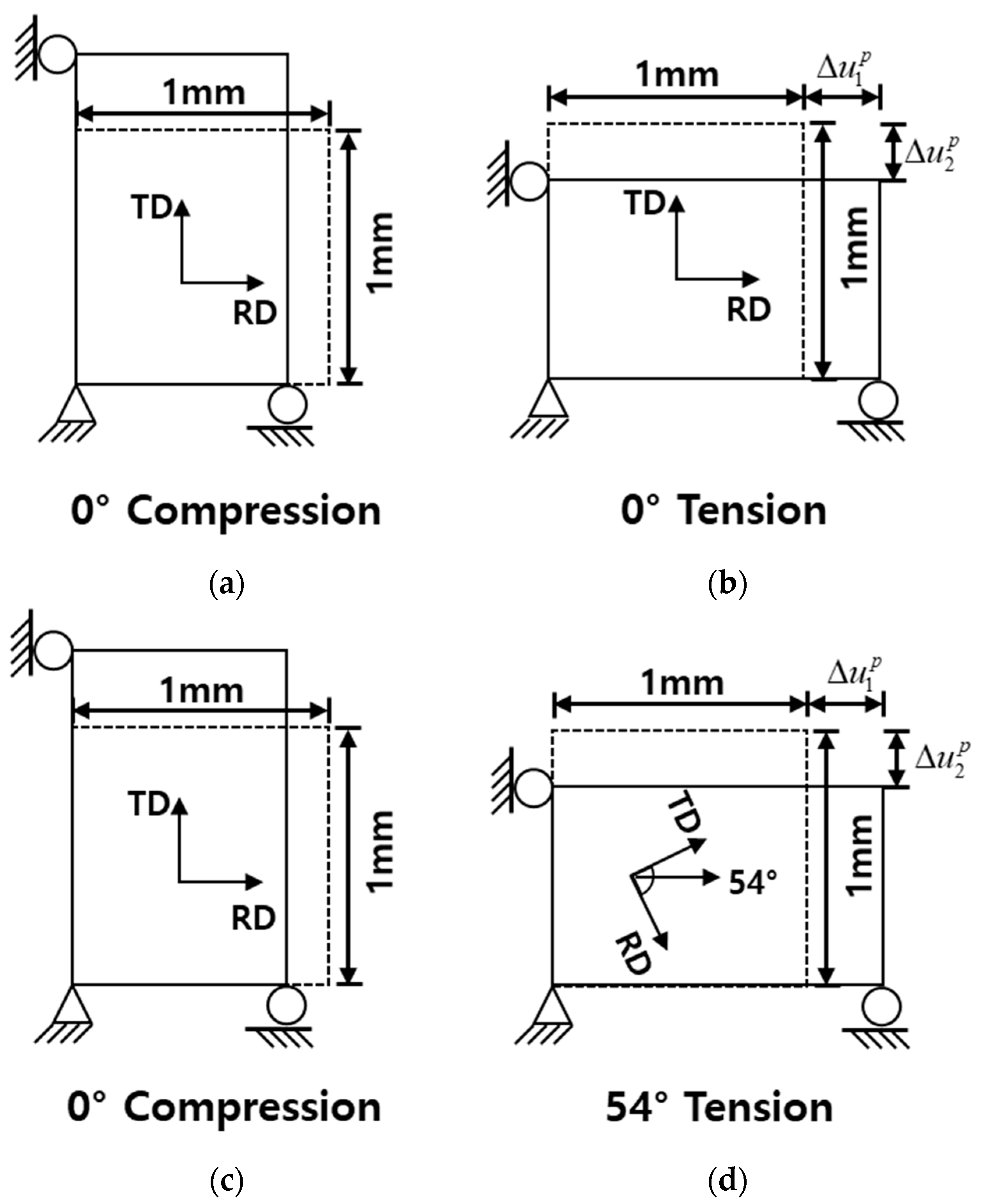
4.1. One Element Analysis

In the one-element analysis, the loading condition consists of a compression-tension (C-T) test. The accuracies of the predicted flow stress and r-value were compared for the investigated numerical algorithms. Two loading paths were simulated for the C-T test. The first path consists of a 5% compression along the rolling direction (RD) followed by a 10% tension along the same direction. This case is denoted as “C5T10R,” where “R” represents the fact that the loading path is a “Reversed” loading condition. During the compression along the RD, the rate of the yield function distortion represented by the transient behavior and Bauschinger effect is maximal in the opposite side of the compressive loading, or tension, along the RD.
The second loading path consists of a 5% compression along the RD followed by a 10% tension at an angle of 54° to the RD. Note that the 54° angle corresponds to the cross-loading state, where the condition h ^ s : s ^ = 0 is satisfied (the exact value of the angle for the cross-loading condition is 54.74°). This case is denoted as “C5T10CR,” where “CR” stands for “cross” loading. This loading path was selected because the cross-loading effect with rotation of the microstructure deviator becomes maximized at the loading direction with the condition.
A four-node shell element with reduced integration in the ABAQUS/Standard, also denoted S4R, was used. The boundary conditions for the above cases are schematically shown in Figure 3.
The r-value along the θ angle with respect to the RD is defined in Equation (59) and calculated via the nodal displacements of an element, according to the following:
r θ = ε w i d t h p ε t h i c k n e s s p = ε 2 p ε 1 p + ε 2 p , w h e r e { ε 1 p = ln ( 1 + Δ u 1 p ) a n d ε 2 p = ln ( 1 + Δ u 2 p ) } ,
where Δ u 1 p and Δ u 2 p are the element nodal displacements along the RD and transverse direction, respectively, during tension, and the superscript “ p ” represents the plastic part of the strain or displacement.
The mechanical properties of the two model materials and the constitutive parameters for the initial yield function and e-HAH model are listed in Table 1 and Table 2, respectively. The model materials “MAT 1” and “MAT 2” have distinctive e-HAH parameters, but other properties, such as elasticity, initial yield function, and isotropic hardening, are identical. For isotropic hardening, the Swift hardening power law, σ ¯ ( ε ¯ ) = K ( e 0 + ε ¯ ) n , is applied for both materials.
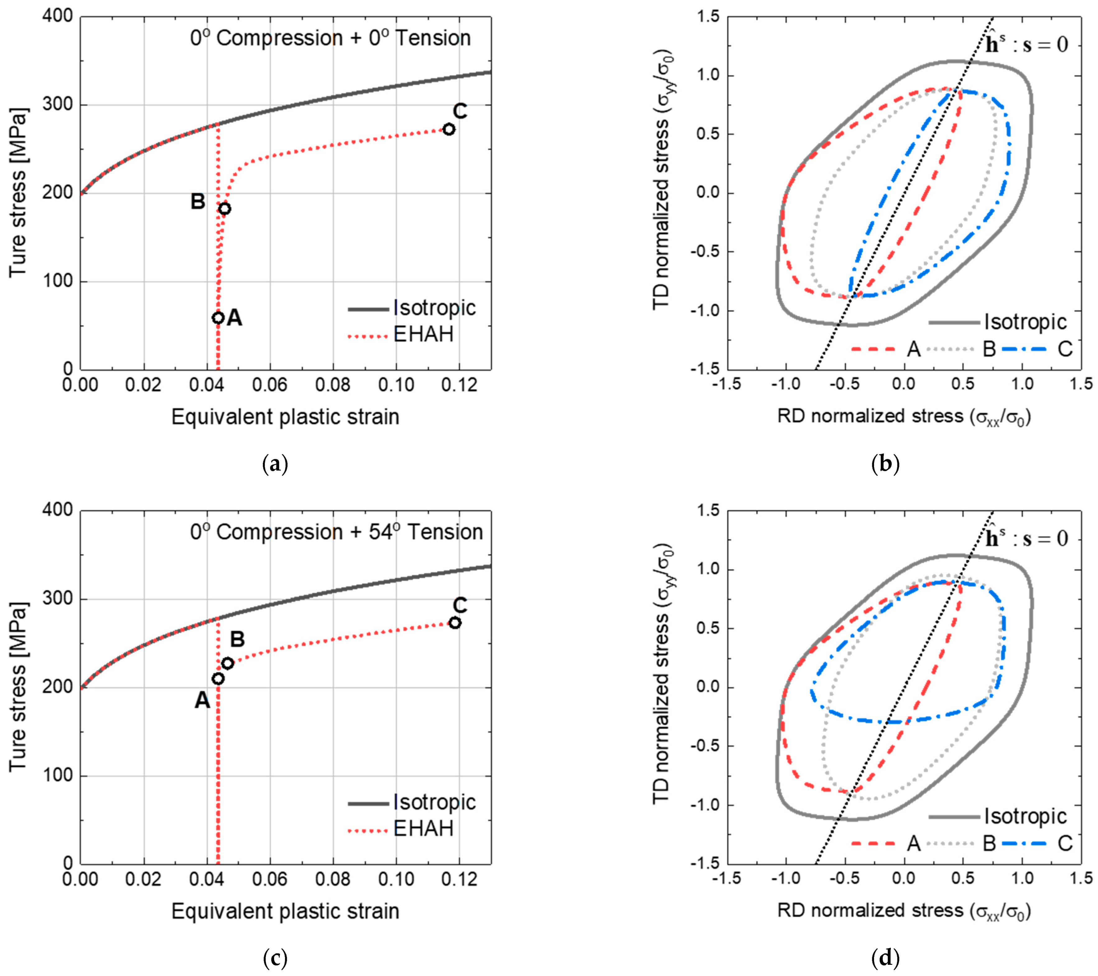
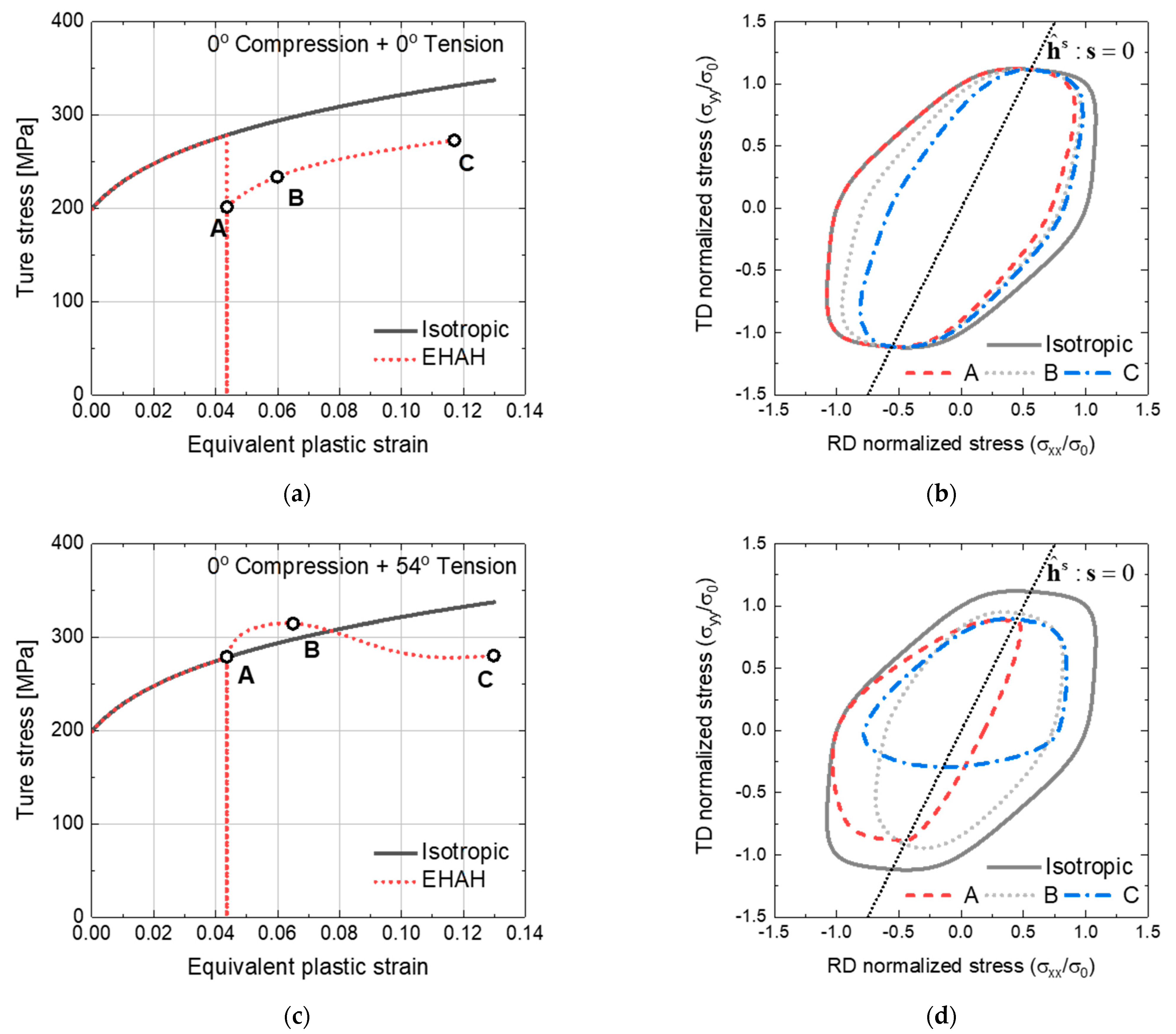
Figure 4 and Figure 5 show the reference flow stress curves and the corresponding evolution of the e-HAH surfaces for MAT 1 and MAT 2, respectively. Since the exact solutions are not available, a reference curve with a sufficiently small time-step is assumed to be exact. The reference flow curves were obtained using the CPM scheme implemented into the dynamic explicit FE ABAQUS/Explicit software with the VUMAT user material subroutine. The average strain increment was set to 2.4 × 10 8 . Figure 4a and Figure 5a illustrate the flow stress curves under the C5T10R loading path, whereas Figure 4c and Figure 5c display the same curves under the C5T10CR loading path. The evolutions of the yield surfaces are provided in Figure 4b and Figure 5b for C5T10R, and in Figure 4d and 
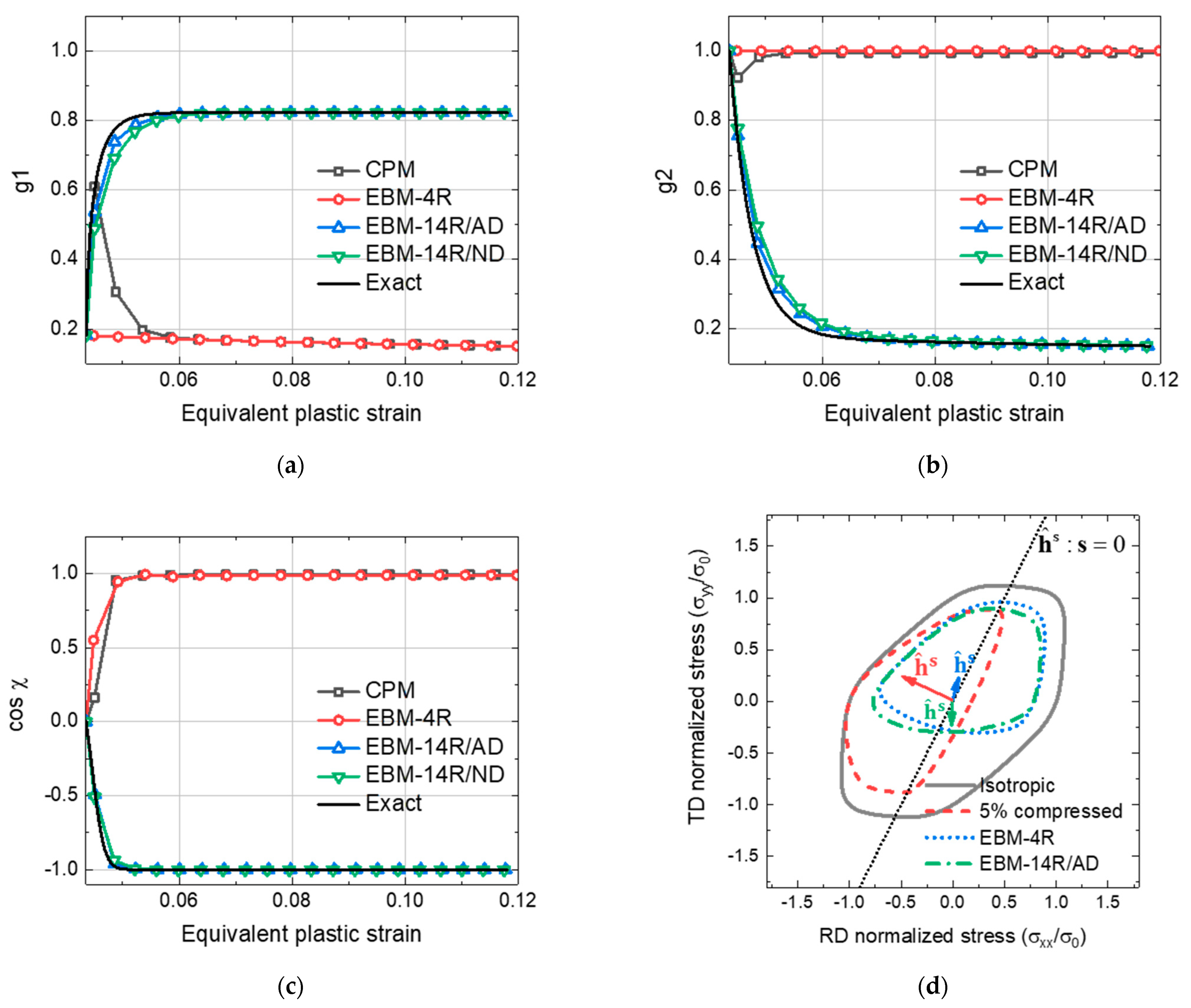
Figure 5d for C510CR. For comparison, the evolutions of the isotropic yield surfaces are also included in the figures. In each figure, three points are marked, namely A, B, and C, where A and C represent the initial and final stress states during the second loading, respectively, whereas B is selected between the two loading points to compare the transient behavior in the second loading path.
Figure 4a,b shows that a significant amount of the Bauschinger effect and permanent softening ( g 4 σ ¯ = 0.8224 σ ¯ ) are represented from the e-HAH parameters of MAT 1 under C5T10R. For C5T10CR, a similar transient behavior and permanent softening were calculated, but the Bauschinger effect (contraction) was found to be much less than for the C5T10R loading path. For MAT 2, the Bauschinger effect is less than in MAT 1 for the C5T10R loading path, though the permanent softening is also pronounced. However, the C5T10CR loading condition showed a very noticeable stress overshoot upon changing the loading path and subsequent softening. Note that MAT 1 and MAT 2 were virtually designed to represent the characteristics of the e-HAH model.
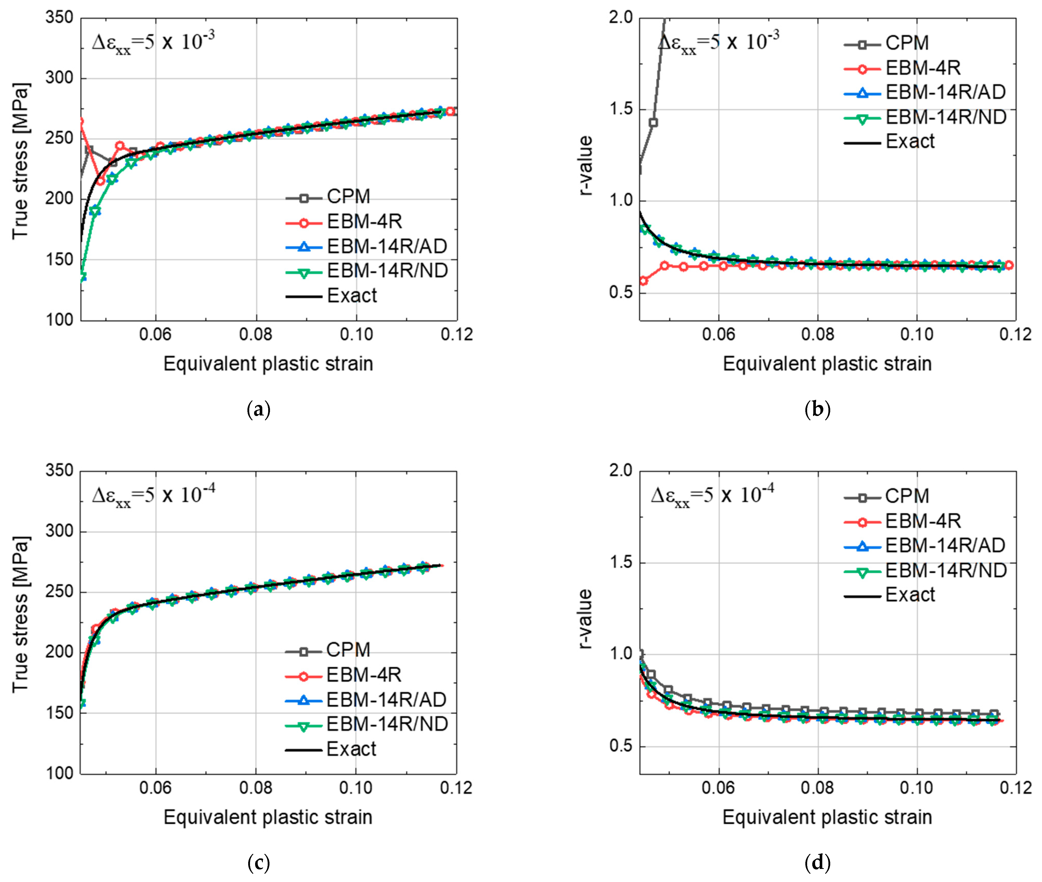
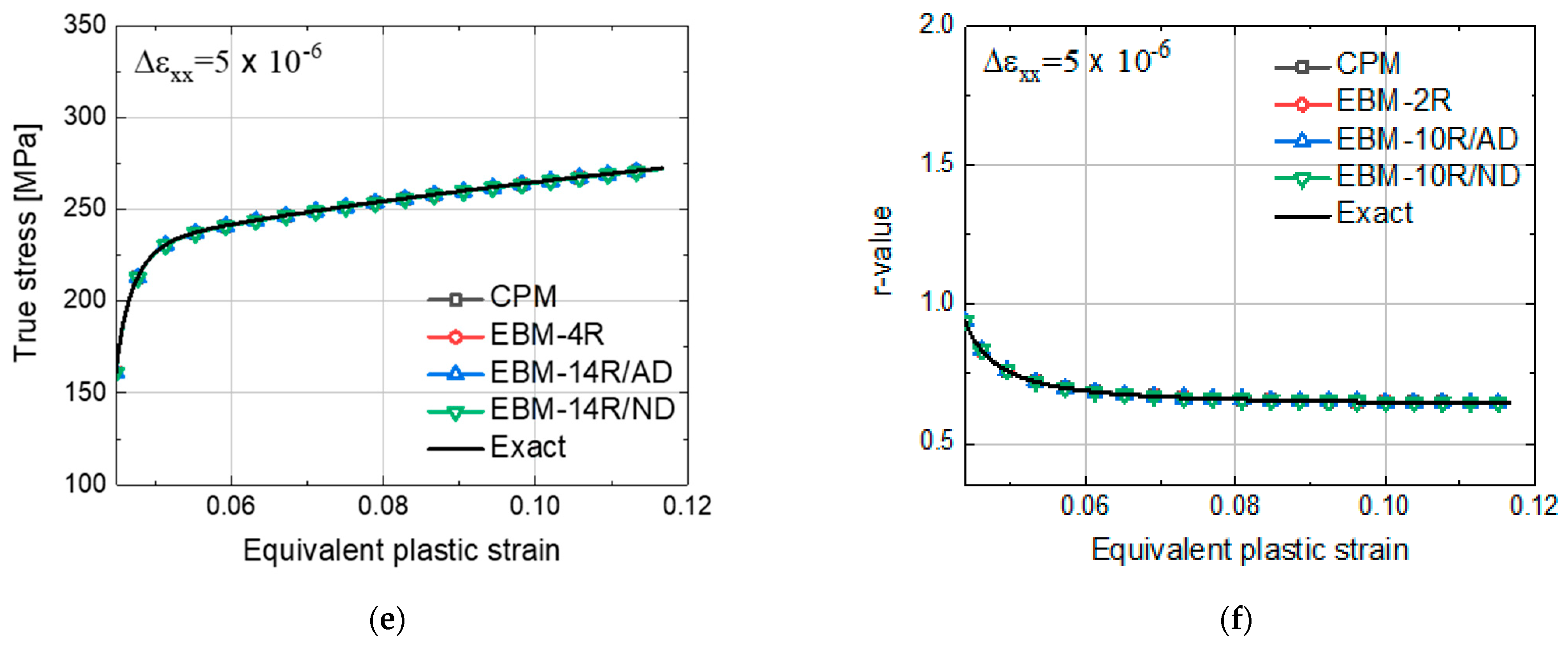
In the following, the accuracy of each investigated stress integration algorithm is assessed with different time increments. The effect of the time-step size on the accuracy of the stress update is evaluated via one-element simulations under the two loading paths. Three different strain increments during tensile loading were considered, i.e., 5.0 × 10 3 , 5.0 × 10 4 , and 5.0 × 10 6 .
From the simulations, the evolution of the flow stress and r-value at the second loading step were evaluated, and the averaged relative errors are reported, using the following equations:
E r r o r σ = 1 N m = 1 N | σ m e x a c t σ m | σ m e x a c t × 100 ( % ) a n d E r r o r r = 1 N m = 1 N | r θ , m e x a c t r θ , m | r θ , m e x a c t × 100 ( % ) ,
where N is the total number of data points used for the error estimations.

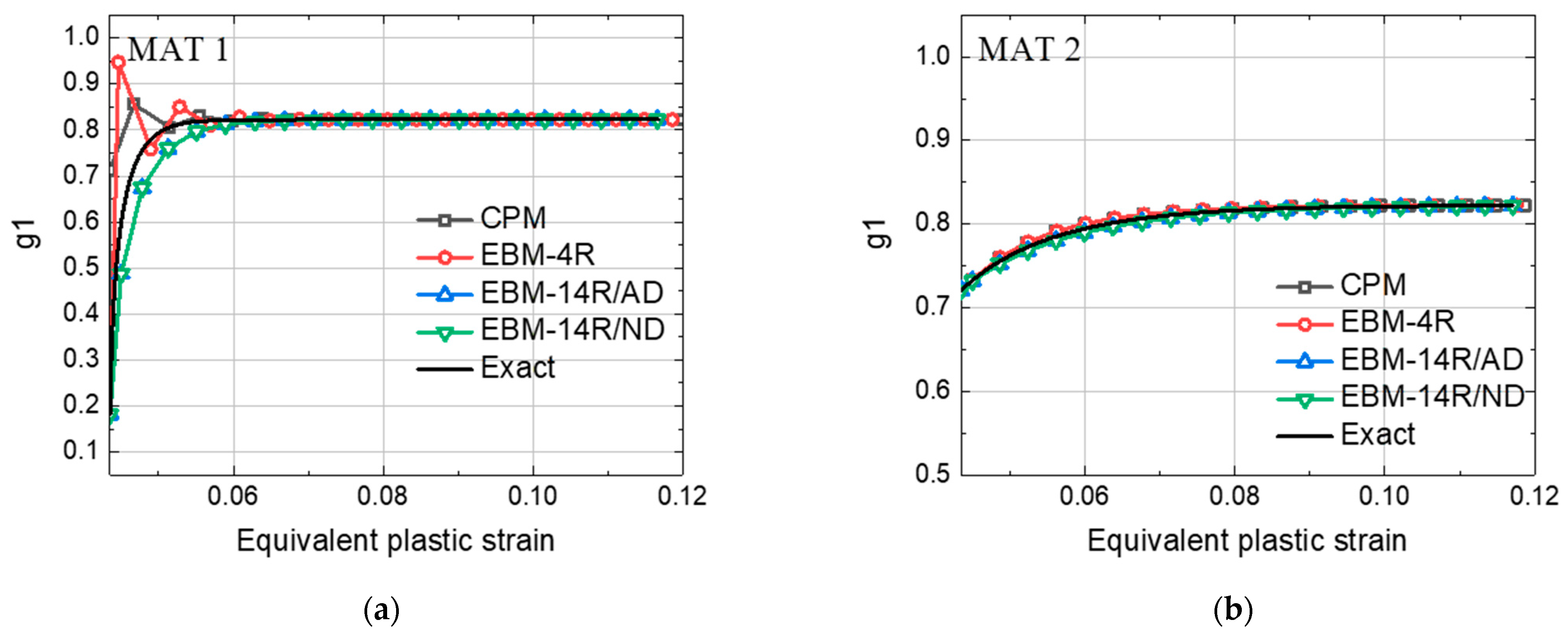
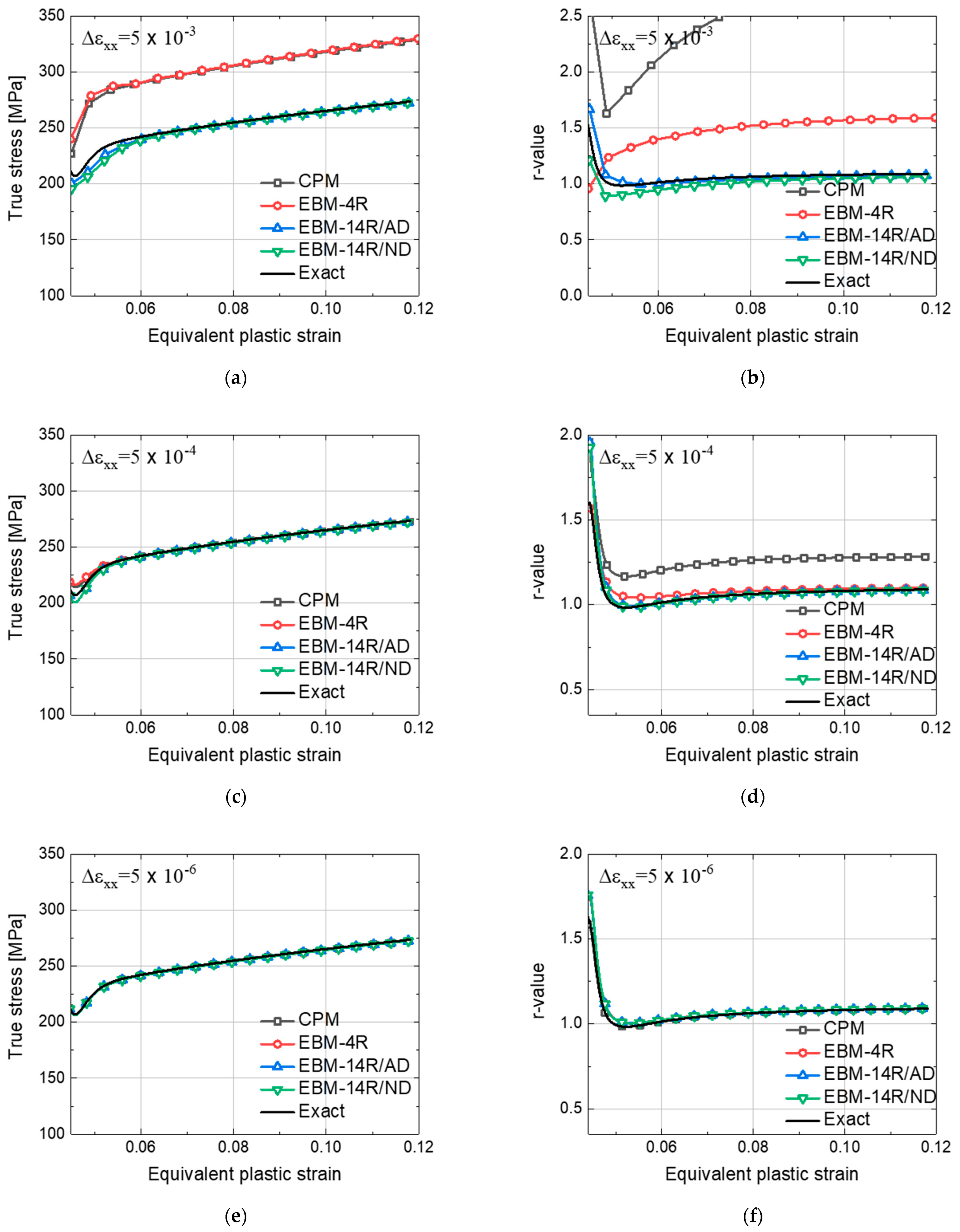
4.1.1. C5T10R Loading Condition

Figure 6 and Figure 7 show the flow stress curves and r-value evolutions of MAT 1 and MAT 2, respectively, under the C5T10R loading path. For this analysis, three different strain increments were applied to each stress integration algorithm. The detailed values, including relative errors and CPU times, are also listed in Table 3 and 
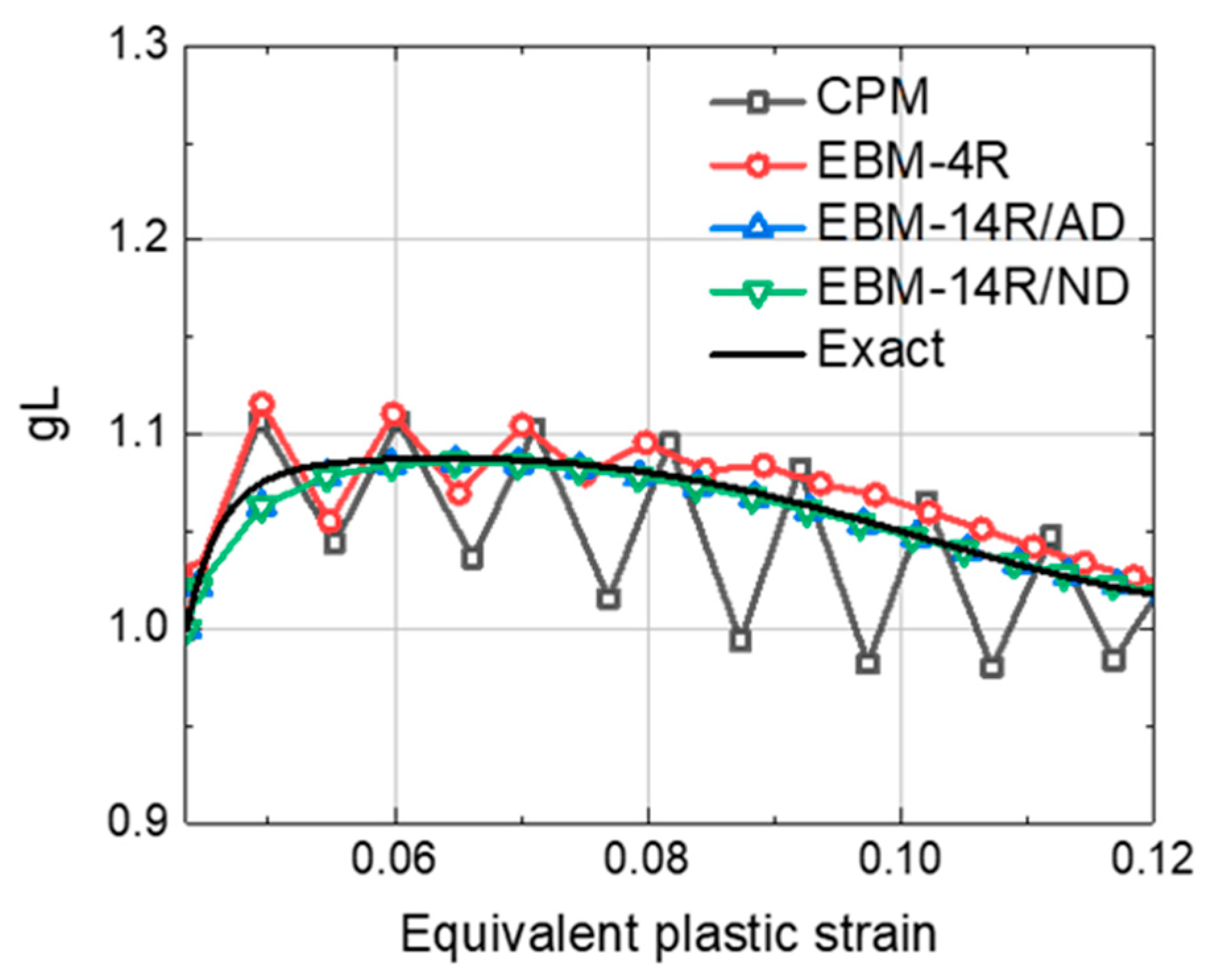
Table 4 for MAT 1 and MAT 2, respectively. At a first glance, all the numerical algorithms investigated seem to yield rather similar results. However, some distinctive features can be observed in the predicted flow curves and r-values. Regarding the method for the yield surface gradient calculation, both approaches based on analytical derivatives (EBM-14R/AD) and finite difference (EBM-14R/ND) predicted almost the same level of accuracy when being implemented into the fully implicit algorithm with 14 residuals. Small differences exist between the two cases in the computational cost measured by the CPU time. Indeed, the EBM-14R/ND scheme using the finite difference method takes ~8% longer CPU time than the EBM-14R/AD scheme using the analytical derivatives.
The effect of the investigated algorithms on the accuracy and stability of the simulations with the e-HAH model grows considerably when the evolution of the yield surface becomes drastic within a given time increment. The flow stress curves predicted by the CPM and EBM-4R schemes show significant oscillations at the early strain range of MAT 1, when the strain increment is large, with Δ ε x x = 5 × 10 3 , as shown in Figure 6a. In contrast, the two algorithms with the same strain increment are stable for MAT 2, which exhibits a lower evolution rate than MAT 1 (Figure 7a). The state variable g 1 controls the transient rate, and Figure 8a shows its oscillations for MAT 1 when the CPM and EBM-4R schemes are used. As expected, the g 1 value of MAT 2 exhibits a stable evolution, even for the CPM and EBM-4R algorithms. In terms of the r-value evolution, the values predicted by the CPM approach show a much lower accuracy for a strain increment of Δ ε x x = 5 × 10 3 . This inaccuracy is attributed to the lack of knowledge of the flow rule as a residual during the algorithmic treatment in the CPM scheme.

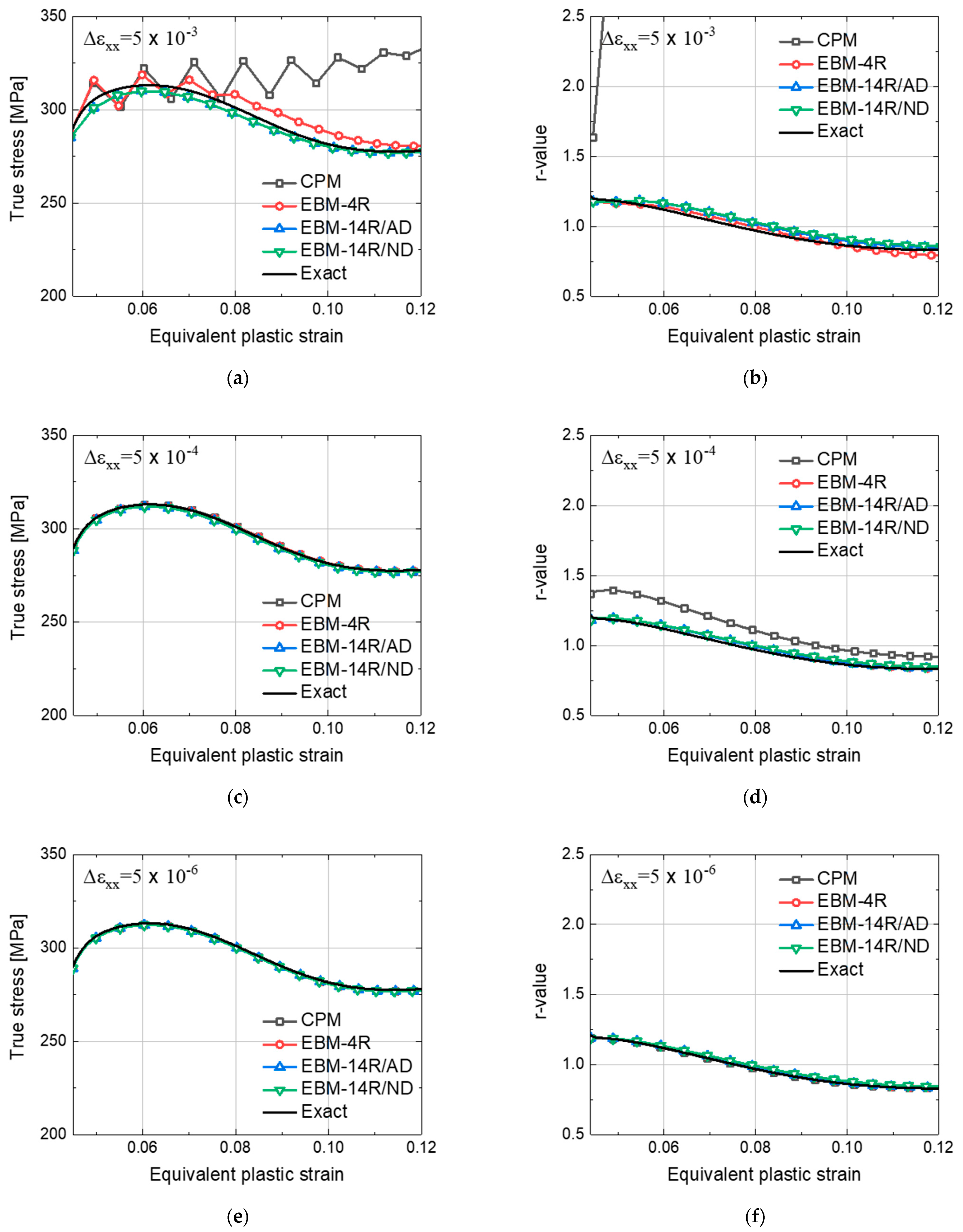
4.1.2. C5T10CR Loading Condition

Figure 9 and Figure 10 show the flow stress and r-value evolutions under the C5T10CR cross-loading path for MAT 1 and MAT 2, respectively. The accuracy and stability of the investigated stress-integration algorithms for MAT 1 and MAT 2 are summarized in Table 5 and Table 6, respectively. Similar to the C5T10R reverse loading path, the overall accuracy for the flow stress and r-values increases upon decreasing the strain increment as expected. However, due to the anisotropic hardening and its orthogonal distortion in the e-HAH model, distinct features can be also noticed, which mostly occur under the large strain increment Δ ε x x = 5 × 10 3 . The evolution of the r-value predicted by the CPM scheme shows an abnormal behavior as can be observed in Figure 9a. This is because the semi-explicit algorithm does not account for the residual minimization for a flow rule. Moreover, as shown in Figure 9a,b, the flow stress and r-value predicted by the CPM and EBM-4R schemes show a different trend with respect to the algorithms using 14 residual—based EBMs. The evolution of the two state variables, g 1 and g 2 , under a strain increment Δ ε x x = 5 × 10 3 are presented in Figure 11a,b. Under this loading path, the transient behavior of CPM and EBM-4R is controlled by g 2 , as the loading path indicator cos χ is negative for both algorithms (Figure 11c). However, for the other algorithms that include the exact solution, cos χ is positive, which leads g 1 to have a major effect on the transient behavior. This circumstance represents the dominant cause behind the abnormally predicted flow stress curve and r-value evolutions for the two algorithms. In other words, the undesirable evolution of the state variables results in significantly deviated stress updates in the e-HAH model, as shown in Figure 11d.
Similar to MAT 1, oscillating flow curves are also predicted by the CPM and EBM-4R approaches for MAT 2 when the time increment is not small enough. In this loading path, the fluctuating flow behavior is attributed to the state variable g L associated with latent hardening (Figure 12). Note that the MAT 2 flow curve is influenced by g L more significantly than for MAT 1, due to the slower evolution of h ^ s .
Regarding the computational time, all investigated numerical algorithms present rather similar values, especially when compared with the much larger differences encountered in the accuracy values, particularly under large strain increments. However, it is important to note that under the C5T10CR loading path, the finite difference gradient—based algorithm (EBM-14R/ND) is characterized by a ~10–15% longer CPU time, compared to the analytical gradient algorithm (EBM-14R/AD).

4.2. Forming Problem: S-Rail Forming and Springback

In this section, the proposed stress integration algorithms are applied to the simulation of large-scale industrial part forming with purely implicit FE software. Though the implicit FE solver was previously employed for large-scale models, this was often limited to simple material constitutive laws, such as isotropic and kinematic hardening. Therefore, this is the first time that the distortional hardening model with cross-hardening or softening (that is, the e-HAH model) is applied to the simulation of industrial forming processes with a static implicit FE solver. By contrast, numerous previous studies have employed the combined dynamic explicit and implicit solvers for complex forming and elastic-driven springback simulations, respectively. In particular, this happens for the case in which the elastic-plasticity constitutive laws become more complex, such as in the present anisotropic hardening model (e-HAH).
In this study, the S-rail part forming and springback simulations were performed as a benchmark for the industrial forming process [45]. The simulations were carried out using the static implicit solver, i.e., the ABAQUS/Standard. From the simulation results, the springback, equilibrium iterations, time increment, and computational time during the forming step were comparatively analyzed using the different CPM, EBM-14R/AD, and EBM-14R/ND algorithms. Real automotive sheet metals, composed of dual-phase steel (DP780) and stainless steel (STS), were employed in the simulations. Note that DP780 exhibits a significant cross-contraction (or softening) behavior under loading path changes, due to the large Baushinger effect induced by its martensitic islands embedded in the ferrite matrix. In contrast, the STS sheet exhibits stress over-shooting or cross-hardening behavior under loading path changes. The material properties and their related model parameters are listed in 
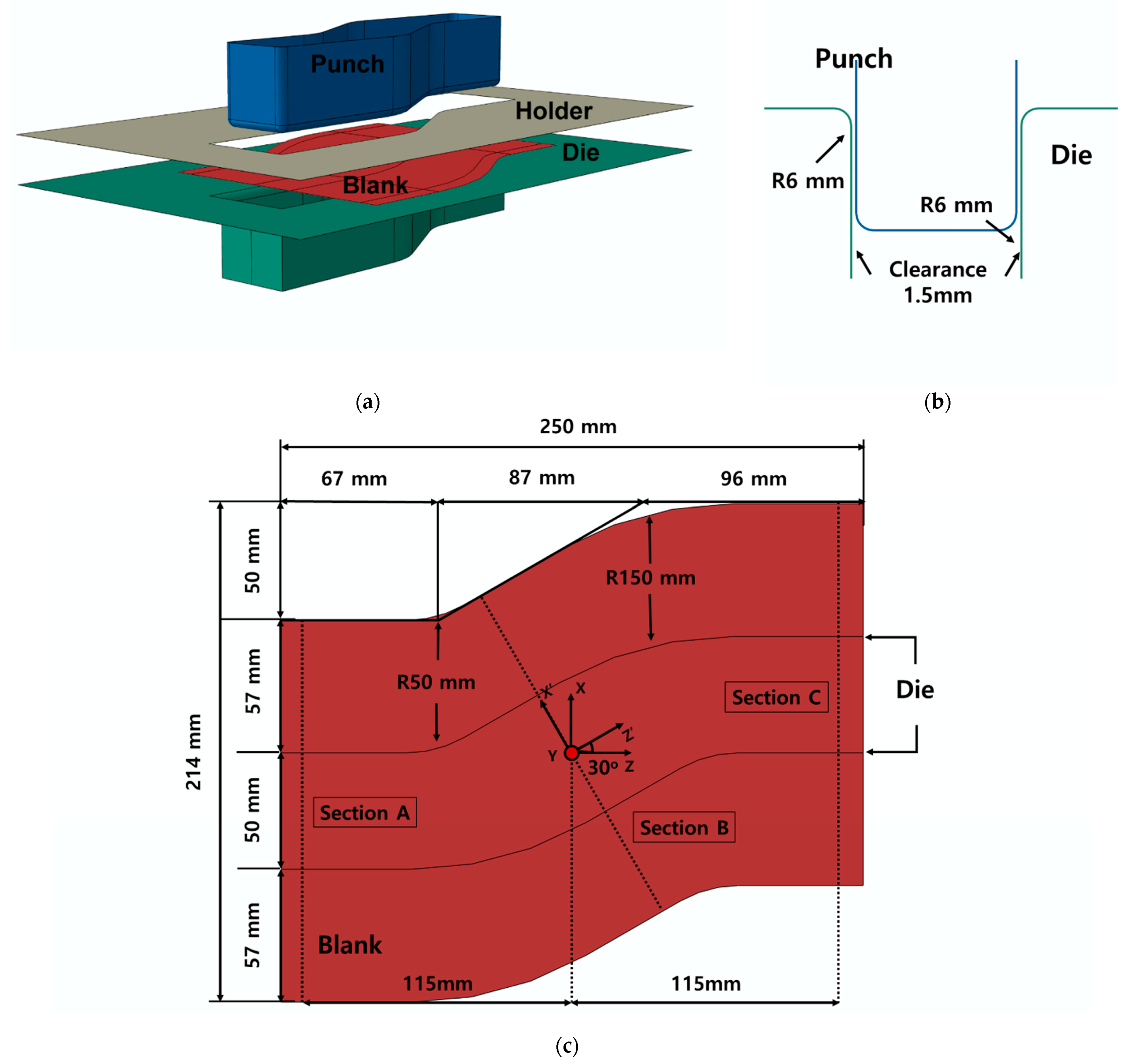
Table 7. The FE model set-up, including tool and sheet dimensions, is presented in Figure 13.
The thickness of the blank sheet was set to 1.2 mm, and a blank holding force of 200 kN was applied during the forming simulation. The friction coefficient between the blank and tools was set to 0.05. A total punch displacement of 37 mm was applied. As for the blank elements, 4264 four-node shell elements with reduced integration (S4R) were used. The simulation consisted of the holding, forming, and springback steps. Springback simulations were conducted by removing the tools after applying constraints on three specific nodes on the X’-Z’ plane to prevent rigid body motion. In other words, the center node was kept fixed, one node on the Z’ axis was constrained along the X’ and Y’ directions, and the last node on the X’ axis was constrained along the Z’ direction. The simulation time for each step was set to one (however, this does not have a physical meaning due to the static implicit FE algorithm. This is a relative measure for the strain increment control for different stress-integration algorithms). The reference, minimum, and maximum time increments for the forming step were set to 5.0 × 10 3 , 1.0 × 10 5 , and 1.0 × 10 2 , respectively.
The sections A, B, and C of the springback are depicted in Figure 13c. Section A and C are on the Z-plane, ± 115 m m away from the center. Section B lies on the Z’-plane, which is rotated by 30° around the Y-axis.
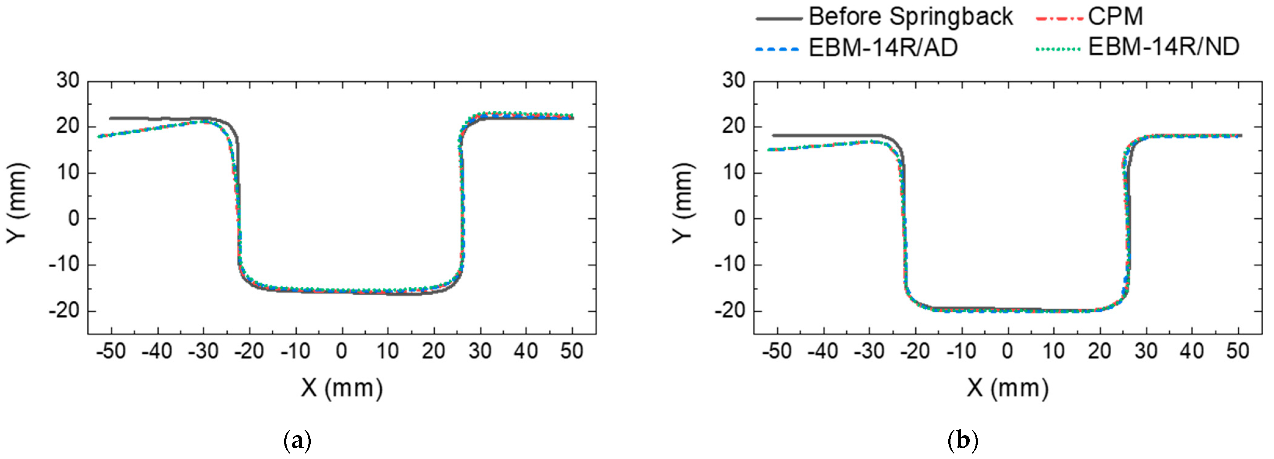
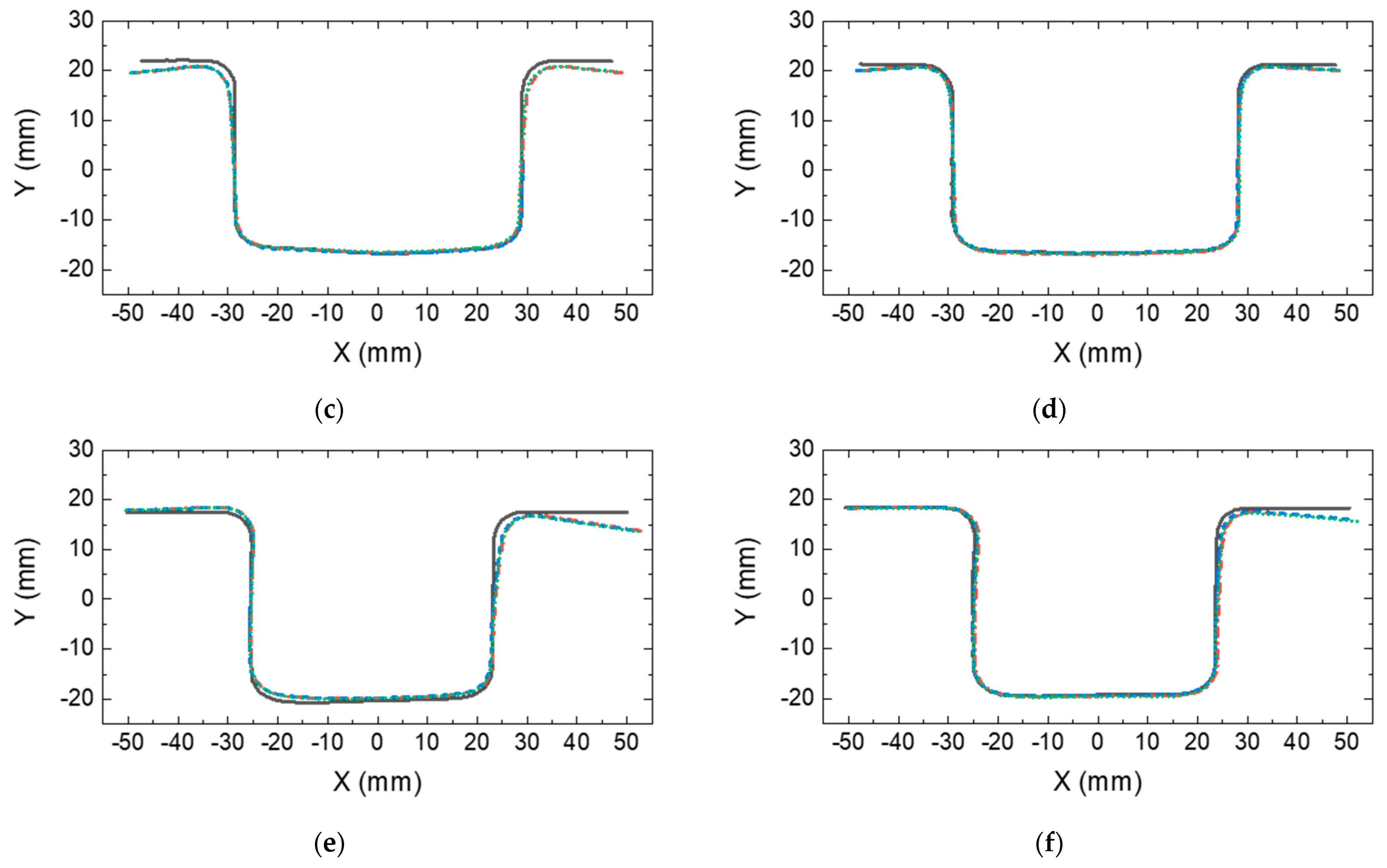
The springback results for section A, B, and C are presented for DP780 and STS in Figure 14. Almost no differences can be observed in the springback results obtained using the different algorithms. This may be due to the automatic time stepping built into the ABAQUS routine and to the fact that the time increment is small enough to have accurate solutions.
The averaged equilibrium iteration number, averaged time increment ( Δ t a v g ), and relative wallclock time are listed in Table 8. The relative wallclock time is normalized with the value calculated using the CPM approach. Pronounced differences in the time increment and calculation time obtained from the different algorithms can be observed. The averaged time increment for CPM is almost half of that of the EBM algorithms. It should be considered that the tangent modulus calculated with CPM is not consistent with the Newton-Raphson method in ABAQUS, which requires a rather smaller time step, compared to the EBM algorithms.
For both materials, the EBM-14R/AD and EBM-14R/ND approaches show a negligible difference in the averaged time increment and average equilibrium iteration number. In other words, the approximate computational cost for global equilibrium calculations in the FE software is similar for the two algorithms. It is thus presumed that the two algorithms have a very similar accuracy under a given time increment. For the STS case, the EBM-14R/AD and EBM-14R/ND methods show similar wallclock times, whereas these times are different for the DP780 case. Indeed, the EBM-14R/ND scheme is approximately 40% slower than the EBM-14R/AD scheme. The difference in convergence speed may be due to the different exponents of the non-quadratic yield function used for the DP780 and STS materials, which also determine the nonlinearity of the yield function evolution.

5. Summary

In this study, a fully implicit stress integration algorithm was developed for the e-HAH anisotropic hardening model. The proposed algorithm is capable of reproducing both cross-hardening and softening under complex loading path changes by introducing the distortional hardening concept. Particularly, the proposed algorithm solves for the complete set of residuals defined from the e-HAH model in the context of the EBM. The major differences between the developed model and previously proposed stress integration algorithms can be summarized as follows.
The developed EBM algorithm is formulated based on a total of 14 residuals for the stress tensor, microstructure deviator tensor, and the whole state variables associated with the e-HAH model. On the contrary, the previous algorithms for the HAH or e-HAH model introduced a partially implicit scheme by considering only a limited number of residuals for greater simplicity. This led to unstable and inaccurate evolutions of the plastic state variables related to the distortions of the yield function under loading path changes.
For calculating the first and second derivatives of the yield surface, which are inevitably required in the formulation of the common predictor-corrector numerical schemes, the present model provides both analytical (EBM-AD) and finite difference—based numerical methods (EBM-ND). The analytical expressions of the e-HAH yield surface are given in the appendix.
The accuracy and robustness of the developed algorithm and its implementation were validated by a one-element analysis and application to a large-size industrial problem. For the one-element analysis, the compression-tension test and compression-cross-tension test were conducted for two representative materials. For the large-size problem, the S-rail benchmark forming and springback simulations were conducted. These validations can be summarized as follows.
The existing semi-explicit CPM and implicit EBM schemes with partially introduced residuals (EBM-4R) resulted in an abnormal evolution of the stress-strain curve or r-value for both the reversed and cross-loading conditions when the strain increment became larger. In contrast, the proposed fully implicit algorithm with the complete set of residuals (EBM-14R) showed stable and accurate results regardless of the investigated strain increments. Moreover, both methods based on analytical and numerical derivatives provided virtually the same accuracy for the EBM-14R algorithm.
For the cross-loading path, the lack of knowledge of the residuals for the evolution of the e-HAH yield surface led to the abnormally wrong rotation of the microstructure deviator h ^ s , which caused undesirable evolutions of the other state variables. This justifies the better accuracy and robustness of the present fully implicit algorithm based on full considerations of the residuals of the e-HAH model.
For the S-rail forming and springback, the investigated algorithms were all successful without divergence, even with the static implicit solver and complicated e-HAH model. However, the EBM—based algorithms required less computational time than the CPM—based one. This is due to the smaller time step determined by the automatic time increment, which resulted from the non-consistent tangent modulus of the CPM algorithm.
Noticeable differences in the averaged time increments and equilibrium iteration number were observed between the EBM-AD and EBM-ND approaches in the S-rail forming simulations. However, the yield surface exponent, which determines the sharpness of the non-quadratic yield function at the bi-axial stress state, played a more dominant role in determining the computational cost in the numerical, derivative—based EBM algorithm.

Author Contributions

Conceptualization, M.-G.L. and S.-C.K.; methodology, H.C. and S.C.; software, H.C. and S.C.; validation, H.C.; investigation, H.C. and S.C.; writing—original draft preparation, H.C. and S.C.; writing—review and editing, M.-G.L.; supervision, M.-G.L.; funding acquisition, M.-G.L. and S.-C.K. All authors have read and agreed to the published version of the manuscript.

Funding

This research received no external funding.

Acknowledgments

The present study has been supported by POSCO, which is greatly appreciated. Also, MGL appreciates partial supports from National Research Foundation (NRF) of Korea (Grant No. 2020R1A2B5B01097417/ 2019R1A5A6099595) and the support of KEIT (No. 20010717).

Conflicts of Interest

The authors declare no conflict of interest.

Appendix A. Analytical Derivatives of e-HAH Model

The first and second derivatives of the e-HAH model are derived analytically as follows.

Appendix A.1. The First Derivatives of Equivalent Stress

Only the derivatives in the case of h ^ s : s ^ > 0 are presented here because similar procedure can be employed for h ^ s : s ^ < 0 .
Φ σ = Φ 1 q { ( ψ ( s ) + ψ ( s p ) ) q 2 1 ( ψ ( s ) ψ ( s ) σ + ψ ( s p ) ψ ( s p ) σ ) + f 2 q ( 2 h ^ s : s ) q 1 2 h ^ s : s σ } ,
Φ h ^ s = Φ 1 q { ( ψ ( s ) + ψ ( s p ) ) q 2 1 ( ψ ( s ) ψ ( s ) h ^ s + ψ ( s p ) ψ ( s p ) h ^ s ) + f 2 q ( 2 h ^ s : s ) q 1 2 s } .
For, h ^ s : s ^ > 0 , Φ g 1 = Φ g 3 = Φ g 4 = Φ g R = 0 .
(Note that this value is changed for h ^ s : s ^ < 0 , Φ g 2 = Φ g 3 = Φ g 4 = Φ g R = 0 )
Φ g 2 = 1 q Φ 1 q { ( 2 h ^ s : s ) 1 q ( 1 g 2 2 ) } ,
Φ g L = Φ 1 q { ( ψ ( s ) + ψ ( s p ) ) q 2 1 ( ψ ( s ) ψ ( s ) g L + ψ ( s p ) ψ ( s p ) g L ) } ψ ( s ) g L = ϕ s ( 1 g L 2 s 0 )   a n d ψ ( s p ) g L = ϕ s ( 4 ( 1 g S ) g L 2 s 0 ) .
Φ g S = Φ 1 q { ( ψ ( s ) + ψ ( s p ) ) q 2 1 ψ ( s p ) ψ ( s p ) g S } w h e r e ψ ( s p ) g S = ϕ s ( 4 g L s 0 ) . .

Appendix A.2. The Second Derivatives of Equivalent Stress

Similarly, only the derivatives in the case of h ^ s : s ^ > 0 are presented here.
2 Φ σ σ = 1 q ( 1 q 1 ) Φ 2 q ( A A ) + 1 q Φ 1 q A σ w i t h A = q Φ q 1 Φ σ B = 2 { ψ ( s ) ψ ( s ) σ + ψ ( s p ) ψ ( s p ) σ } A σ = q 2 ( q 2 1 ) { ψ ( s ) 2 + ψ ( s p ) 2 } q 2 2 B B + q 2 { ψ ( s ) 2 + ψ ( s p ) 2 } q 2 1 B σ + f 2 q q ( q 1 ) ( 2 h ^ s : s σ ) ( 2 h ^ s : s σ ) B σ = 2 { ψ ( s ) σ ψ ( s ) σ + ψ ( s p ) σ ψ ( s p ) σ + ψ ( s ) 2 ψ ( s ) σ σ + ψ ( s p ) 2 ψ ( s p ) σ σ } 2 ψ ( s ) σ σ = ( s s : s σ ) T : ( 2 ϕ s s ) : ( s s : s σ ) 2 ψ ( s p ) σ σ = ( s p s : s σ ) T : ( 2 ϕ s p s p ) : ( s p s : s σ ) ,
2 Φ σ h ^ s = ( 1 q ) Φ 1 Φ σ Φ h ^ s + 1 q Φ 1 q A h ^ s w i t h A h ^ s = q 2 ( q 2 1 ) { ψ ( s ) 2 + ψ ( s p ) 2 } q 2 2 B B h ^ s + q 2 { ψ ( s ) 2 + ψ ( s p ) 2 } q 2 1 B h ^ s + f 2 q q ( 2 h ^ s : s ) q 1 2 ( s σ ) T + f 2 q q ( q 1 ) ( 2 h ^ s : s ) q 2 ( 2 h ^ s : s σ ) 2 s B h ^ s = 2 { ψ ( s ) ψ ( s ) h ^ s + ψ ( s p ) ψ ( s p ) h ^ s } B h ^ s = 2 { ψ ( s ) σ ψ ( s ) h ^ s + ψ ( s p ) σ ψ ( s p ) h ^ s + ψ ( s ) 2 ψ ( s ) σ h ^ s + ψ ( s p ) 2 ψ ( s p ) σ h ^ s } 2 ψ ( s ) σ h ^ s = ( s σ ) T : { ( 1 1 g L ) H ( ϕ s : h ^ s ) I 4 + h ^ s ϕ s } + ( s s : s σ ) T : 2 ϕ s s : s h ^ s 2 ψ ( s p ) σ h ^ s = ( s σ ) T : { ( 4 ( 1 g S ) g L ) H ( ϕ s : h ^ s ) I 4 + h ^ s ϕ s } + ( s p s : s σ ) T : 2 ϕ s p s p : s p h ^ s
2 Φ σ g 2 = ( 1 q q ) Φ q A Φ g 2 + 1 q Φ 1 q { q ( 2 h ^ s : s ) q 1 g 2 2 } ( 2 h ^ s : s σ ) ,
2 Φ σ g L = ( 1 q q ) Φ q Φ g L A + 1 q Φ 1 q A g L w i t h A g L = q 2 ( q 2 1 ) { ψ ( s ) 2 + ψ ( s p ) 2 } q 2 2 B B g L + q 2 { ψ ( s ) 2 + ψ ( s p ) 2 } q 2 1 B g L B g L = 2 { ψ ( s ) ψ ( s ) g L + ψ ( s p ) ψ ( s p ) g L } B g L = 2 { ψ ( s ) σ ψ ( s ) g L + ψ ( s p ) σ ψ ( s p ) g L + ψ ( s ) 2 ψ ( s ) σ g L + ψ ( s p ) 2 ψ ( s p ) σ g L } 2 ψ ( s ) σ g L = ϕ s : ( 1 g L 2 s 0 s ) : s σ 2 ψ ( s p ) σ g L = ϕ s p : ( 4 ( 1 g S ) g L 2 s 0 s ) : s σ .
2 Φ σ g S = ( 1 q q ) Φ q Φ g S A + 1 q Φ 1 q A g S w i t h A g S = q 2 ( q 2 1 ) { ψ ( s ) 2 + ψ ( s p ) 2 } q 2 2 B B g S + q 2 { ψ ( s ) 2 + ψ ( s p ) 2 } q 2 1 B g S B g S = 2 ψ ( s p ) ψ ( s p ) g S B g S = 2 { ψ ( s p ) σ ψ ( s p ) g S + ψ ( s p ) 2 ψ ( s p ) σ g S } 2 ψ ( s p ) σ g S = ϕ s p : ( 4 g L s 0 s ) : s σ .

Appendix A.3. The First Derivatives of the State Variables g i ( i = 1 ~ 4 , L , S , R )

g 1 ( g 1 ε ¯ ) = { k 2 ( h ^ s : s 0 ) k 1 g 4 g 1 2 ( h ^ s : s < 0 ) .
g 4 ( g 1 ε ¯ ) = { 0 ( h ^ s : s 0 ) k 1 g 1 ( h ^ s : s < 0 ) .
ε ¯ ( g 1 ε ¯ ) = { k 2 k 3 σ ¯ ( 0 ) σ ¯ ( ε ¯ ) 2 σ ¯ ( ε ¯ ) ( h ^ s : s 0 ) 0   ( h ^ s : s < 0 ) .
g 2 ( g 2 ε ¯ ) = { k 1 g 3 g 2 2 ( h ^ s : s 0 ) k 2 ( h ^ s : s < 0 ) .
g 4 ( g 2 ε ¯ ) = { k 1 g 2 ( h ^ s : s 0 ) 0   ( h ^ s : s < 0 ) .
ε ¯ ( g 2 ε ¯ ) = { 0   ( h ^ s : s 0 ) k 2 k 3 σ ¯ ( 0 ) σ ¯ ( ε ¯ ) 2 σ ¯ ( ε ¯ )   ( h ^ s : s < 0 ) .
g 3 ( g 3 ε ¯ ) = { 0 ( h ^ s : s 0 ) k 5 ( h ^ s : s < 0 ) .
g 4 ( g 4 ε ¯ ) = { k 5 ( h ^ s : s 0 ) 0 ( h ^ s : s < 0 ) .
g L ( g L ε ¯ ) = k L .
ε ¯ ( g L ε ¯ ) = k L ( L ( 1 cos 2 χ ) + cos 2 χ 1 ) ( σ ¯ ( ε ¯ ) σ ¯ ( 0 ) σ ¯ ( ε ¯ ) 2 ) .
σ ( g L ε ¯ ) = k L ( σ ¯ ( ε ¯ ) σ ¯ ( 0 ) σ ¯ ( ε ¯ ) ) ( 1 L ) cos χ L ( 1 cos 2 χ ) + cos 2 χ × H s : s ( I 4 1 3 ( I I ) ) : ( h ^ s h ^ s : s ( s : s ) s ) .
h ^ s ( g L ε ¯ ) = k L ( σ ¯ ( ε ¯ ) σ ¯ ( 0 ) σ ¯ ( ε ¯ ) ) ( 1 L ) cos χ L ( 1 cos 2 χ ) + cos 2 χ H s : s s .
g S ( g S ε ¯ ) = k S .
σ ( g S ε ¯ ) = 2 k S ( S 1 ) ( H h ^ s : s ( s : s ) ) ( I 4 1 3 ( I I ) ) : ( h ^ s h ^ s : s ( s : s ) s ) .
h ^ s ( g S ε ¯ ) = 2 k S ( S 1 ) H h ^ s : s ( s : s ) s .
g S ( g S ε ¯ ) = k S .
σ ( g S ε ¯ ) = 2 k S ( S 1 ) ( H h ^ s : s ( s : s ) ) ( I 4 1 3 ( I I ) ) : ( h ^ s h ^ s : s ( s : s ) s ) .
h ^ s ( g S ε ¯ ) = 2 k S ( S 1 ) H h ^ s : s ( s : s ) s .
g R ( g R ε ¯ ) = k R .
σ ( g R ε ¯ ) = 2 k R k R ( H h ^ s : s ( s : s ) ) ( I 4 1 3 ( I I ) ) : ( h ^ s h ^ s : s ( s : s ) s ) .
h ^ s ( g R ε ¯ ) = 2 k R k R H h ^ s : s ( s : s ) s .

Appendix A.4. The First Derivatives of the State Variables h ^ s

The value sgn ( cos ( χ ) ) used in this section is defined as follows.
sgn ( cos ( χ ) ) = { + 1 ( h ^ s : s 0 ) 1 ( h ^ s : s < 0 ) .
g R ( h ^ s ε ¯ ) = k sgn ( cos ( χ ) ) ( s ^ cos ( χ ) h ^ s ) .
σ ( h ^ s ε ¯ ) = k sgn ( cos χ ) ( | cos χ | 1 / z + g R ) × [ 1 H 1 s : s { I 4 ( s s ) s : s H h ^ ( h ^ s h ^ s : s ( s : s ) s ) } : ( I 4 1 3 ( I I ) ) + ( s ^ cos χ h ^ s ) 1 z sgn ( cos χ ) | cos χ | 1 / z 1 H s : s ( h ^ s h ^ s : s ( s : s ) s ) ] .
h ^ s ( h ^ s ε ¯ ) = k sgn ( cos χ ) [ ( | cos χ | 1 / z + g R ) H s : s { h ^ s s + ( h ^ s : s ) I 4 } + 1 z sgn ( cos χ ) | cos χ | 1 / z 1 ( s ^ cos χ h ^ s ) H s : s s ] .

Appendix B. Numerical Derivatives of e-HAH Model

In the previous study by Choi and Yoon [57], the central finite difference method was adopted for numerical derivatives because of its faster convergence and lower error. Therefore, in this study the same finite difference was employed. For the step size decision for numerical differentiation, the scaled stress space idea was used [60]. For the sake of simplicity, the Voigt notation under the plane stress condition was used. The step sizes for each state variables were defined based on common step size as follows.
δ σ i = σ a b σ a b × a δ h ^ s i = h ^ s a b h ^ s a b × a δ g m = g m × a ,    ( m = 1 ~ 4 , L , S , R ) δ ε ¯ = ε ¯ × a .
In this study, a = 1.0 × 1 0 6 was employed for the calculation. Examples of the first and second derivatives with respect to stress are shown as follows.
Φ σ 3 Φ ( σ 1 , σ 2 , σ 3 + δ σ 3 ) Φ ( σ 1 , σ 2 , σ 3 δ σ 3 ) 2 δ σ 3 .
2 Φ σ 3 σ 3 Φ ( σ 1 , σ 2 , σ 3 + δ σ 3 ) 2 Φ ( σ 1 , σ 2 , σ 3 ) + Φ ( σ 1 , σ 2 , σ 3 δ σ 3 ) ( δ σ 3 ) 2 .
2 Φ σ 1 σ 3 1 4 δ σ 1 δ σ 3 [ Φ ( σ 1 + δ σ 1 , σ 2 , σ 3 + δ σ 3 ) Φ ( σ 1 δ σ 1 , σ 2 , σ 3 + δ σ 3 ) Φ ( σ 1 + δ σ 1 , σ 2 , σ 3 δ σ 3 ) + Φ ( σ 1 δ σ 1 , σ 2 , σ 3 δ σ 3 ) ] .
Similarly, all other derivatives associated to the e-HAH can be calculated. There is a remark for using numerical derivatives with respect to g i ( i = 1 ~ 4 , L , S , R ) . g values have admissible range of value, e.g., 0 < g 1 1 . When g 1 equals 0 or 1, the numerical derivatives cannot be defined. In this case, the forward or backward difference method can be applied.

Appendix C. Yld2000-2d Yield Function

A non-quadratic anisotropic yield function proposed by Barlat et al. [62,63] is formulated as follows.
2 Φ a = | X 1   X 2 | a + | 2 X 2 + X 1 | a + | 2 X 1 + X 2 | a .
where X i and X i ( i = 1 , 2 ) are the principal values of linearly transformed Cauchy stress. For simplicity, the Voigt notation is used for the formulation. The relationship between X ( o r X ) and σ is as follows.
X = C s = C T σ = L   σ X = C s = C T σ = L σ .
The components of linear transformation matrixes consist of the anisotropic coefficients α 1 ~ 8 as follows.
L   = 1 3 [ 2 α 1 α 1 0 α 2 2 α 2 0 0 0 3 α 7 ] L   = 1 9 [ 2 α 3 + 2 α 4 + 8 α 5 2 α 6 α 3 4 α 4 4 α 5 + 4 α 6 0 4 α 3 4 α 4 4 α 5 + α 6 2 α 3 + 8 α 4 + 2 α 5 2 α 6 0 0 0 9 α 8 ] .

References

  1. Sowerby, R.; Uko, D.K. A review of certain aspects of the Bauschinger effect in metals. Mater. Sci. Eng. 1979, 41, 43–58. [Google Scholar] [CrossRef]
  2. Bate, P.S.; Wilson, D.V. Analysis of the Bauschinger effect. Acta Metall. 1986, 34, 1097–1105. [Google Scholar] [CrossRef]
  3. Yoshida, F.; Uemori, T. A model of large-strain cyclic plasticity describing the Bauschinger effect and workhardening stagnation. Int. J. Plast. 2002, 18, 661–686. [Google Scholar] [CrossRef]
  4. Boger, R.K.; Wagoner, R.H. Continuous, large strain, tension/compression testing of sheet material. Int. J. Plast. 2005, 21, 2319–2343. [Google Scholar] [CrossRef]
  5. Mamun, A.A.; Moat, R.J. Origin of the Bauschinger effect in a polycrystalline material. Mater. Sci. Eng. A 2017, 707, 576–584. [Google Scholar] [CrossRef] [Green Version]
  6. Li, K.P.; Carden, W.P. Simulation of springback. Int. J. Mech. Sci. 2002, 44, 103–122. [Google Scholar] [CrossRef]
  7. Lee, M.G.; Kim, D. Spring-back evaluation of automotive sheets based on isotropic-kinematic hardening laws and non-quadratic anisotropic yield functions, part III: Applications. Int. J. Plast. 2005, 21, 915–953. [Google Scholar] [CrossRef]
  8. Lee, M.G.; Kim, D. A practical two-surface plasticity model and its application to spring-back prediction. Int. J. Plast. 2007, 23, 1189–1212. [Google Scholar] [CrossRef]
  9. Wagoner, R.H.; Lim, H. Advanced issues in springback. Int. J. Plast. 2013, 45, 3–20. [Google Scholar] [CrossRef]
  10. Franciosi, P. The concepts of latent hardening and strain hardening in metallic single crystals. Acta Metall. 1985, 33, 1601–1612. [Google Scholar] [CrossRef]
  11. Schmitt, J.H.; Shen, E.L. A parameter for measuring the magnitude of a change of strain path: Validation and comparison with experiments on low carbon steel. Int. J. Plast. 1994, 10, 535–551. [Google Scholar] [CrossRef]
  12. Vincze, G.; Barlat, F. Experiments and modeling of low carbon steel sheet subjected to double strain path changes. Metall. Mater. Trans. A 2013, 44, 4475–4479. [Google Scholar] [CrossRef] [Green Version]
  13. Ha, J.; Lee, M.G. Strain hardening response and modeling of EDDQ and DP780 steel sheet under non-linear strain path. Mech. Mater. 2013, 64, 11–26. [Google Scholar] [CrossRef]
  14. Wen, W.; Borodachenkova, M. Mechanical behavior of low carbon steel subjected to strain path changes: Experiments and modeling. Acta Mater. 2016, 111, 305–314. [Google Scholar] [CrossRef] [Green Version]
  15. Zaman, S.B.; Barlat, F. Deformation-induced anisotropy of uniaxially prestrained steel sheets. Int. J. Solids Struct. 2018, 134, 20–29. [Google Scholar] [CrossRef]
  16. Sun, L.; Wagoner, R.H. Proportional and non-proportional hardening behavior of dual-phase steels. Int. J. Plast. 2013, 45, 174–187. [Google Scholar] [CrossRef]
  17. Liao, J.; Sousa, J.A. Mechanical, microstructural behaviour and modelling of dual phase steels under complex deformation paths. Int. J. Plast. 2017, 93, 269–290. [Google Scholar] [CrossRef]
  18. Ha, J.; Lee, J. Investigation of plastic strain rate under strain path changes in dual-phase steel using microstructure—based modeling. Int. J. Plast. 2017, 93, 89–111. [Google Scholar] [CrossRef]
  19. Prager, W. A new methods of analyzing stresses and strains in work hardening plastic solids. J. Appl. Mech. (ASME) 1956, 23, 493–496. [Google Scholar] [CrossRef]
  20. Ziegler, H. A modification of Prager’s hardening rule. Q. Appl. Math. 1959, 17, 55–65. [Google Scholar] [CrossRef] [Green Version]
  21. Armstrong, P.J.; Frederick, C.O. A Mathematical Representation of the Multiaxial Bauschinger Effect; Central Electricity Generating Board and Berkeley Nuclear Laboratories, Research & Development Department: Berkeley, CA, USA, 1966. [Google Scholar]
  22. Chaboche, J.L. Time-independent constitutive theories for cyclic plasticity. Int. J. Plast. 1986, 2, 149–188. [Google Scholar] [CrossRef]
  23. Ohno, N.; Wang, J.D. Kinematic hardening rules with critical state of dynamic recovery, part I: Formulation and basic features for ratchetting behavior. Int. J. Plast. 1993, 9, 375–390. [Google Scholar] [CrossRef]
  24. Yoshida, F.; Uemori, T. Elastic-plastic behavior of steel sheets under in-plane cyclic tension-compression at large strain. Int. J. Plast. 2002, 18, 633–659. [Google Scholar] [CrossRef]
  25. Chung, K.; Lee, M.G. Spring-back evaluation of automotive sheets based on isotropic-kinematic hardening laws and non-quadratic anisotropic yield functions: Part I: Theory and formulation. Int. J. Plast. 2005, 21, 861–882. [Google Scholar] [CrossRef]
  26. Ortiz, M.; Popov, E.P. Distortional hardening rules for metal plasticity. J. Eng. Mech. 1983, 109, 1042–1057. [Google Scholar] [CrossRef]
  27. Feigenbaum, H.P.; Dafalias, Y.F. Directional distortional hardening in metal plasticity within thermodynamics. Int. J. Solids Struct. 2007, 44, 7526–7542. [Google Scholar] [CrossRef]
  28. Feigenbaum, H.P.; Dafalias, Y.F. Simple model for directional distortional hardening in metal plasticity within thermodynamics. J. Eng. Mech. 2008, 134, 730–738. [Google Scholar] [CrossRef]
  29. Teodosiu, C.; Hu, Z. Evolution of the intragranular microstructure at moderate and large strains: Modelling and computational significance. In Simulation of Materials Processing: Theory, Methods and Applications; Balkema: Rotterdam, The Netherlands, 1995; pp. 173–182. [Google Scholar]
  30. François, M. A plasticity model with yield surface distortion for non proportional loading. Int. J. Plast. 2001, 17, 703–717. [Google Scholar] [CrossRef] [Green Version]
  31. Badreddine, H.; Yue, Z.M. Modeling of the induced plastic anisotropy fully coupled with ductile damage under finite strains. Int. J. Solids Struct. 2017, 108, 49–62. [Google Scholar] [CrossRef]
  32. Qin, J.; Holmedal, B. A combined isotropic, kinematic and distortional hardening model for aluminum and steels under complex strain-path changes. Int. J. Plast. 2018, 101, 156–169. [Google Scholar] [CrossRef]
  33. Tari, D.G.; Worswick, M.J. Mechanical response of AZ31B magnesium alloy: Experimental characterization and material modeling considering proportional loading at room temperature. Int. J. Plast. 2014, 55, 247–267. [Google Scholar] [CrossRef]
  34. Choi, H.J.; Lee, K.J. Effect of evolutionary anisotropy on earing prediction in cylindrical cup drawing. JOM 2017, 69, 915–921. [Google Scholar] [CrossRef]
  35. Abedini, A.; Butcher, C. Application of an evolving non-associative anisotropic-asymmetric plasticity model for a rare-earth magnesium alloy. Metals 2018, 8, 1013. [Google Scholar] [CrossRef] [Green Version]
  36. Park, T.; Abu-Farha, F. An evolutionary yield function model based on plastic work and non-associated flow rule. Metals 2019, 9, 611. [Google Scholar] [CrossRef] [Green Version]
  37. Barlat, F.; Gracio, J.J. An alternative to kinematic hardening in classical plasticity. Int. J. Plast. 2011, 27, 1309–1327. [Google Scholar] [CrossRef]
  38. Barlat, F.; Ha, J. Extension of homogeneous anisotropic hardening model to cross-loading with latent effects. Int. J. Plast. 2013, 46, 130–142. [Google Scholar] [CrossRef]
  39. Barlat, F.; Vincze, G. Enhancements of homogenous anisotropic hardening model and application to mild and dual-phase steels. Int. J. Plast. 2014, 58, 201–218. [Google Scholar] [CrossRef]
  40. Lee, J.W.; Lee, M.G. Finite element modeling using homogeneous anisotropic hardening and application to spring-back prediction. Int. J. Plast. 2012, 29, 13–41. [Google Scholar] [CrossRef]
  41. Lee, J.Y.; Lee, J.W. An application of homogeneous anisotropic hardening to springback prediction in pre-strained U-draw/bending. Int. J. Solids Struct. 2012, 49, 3562–3572. [Google Scholar] [CrossRef] [Green Version]
  42. Choi, J.; Lee, J. Evaluation of springback for DP980 S rail using anisotropic hardening models. JOM 2016, 68, 1850–1857. [Google Scholar] [CrossRef]
  43. Badr, O.M.; Rolfe, B. Applying a new constitutive model to analyse the springback behaviour of titanium in bending and roll forming. Int. J. Mech. Sci. 2017, 128, 389–400. [Google Scholar] [CrossRef]
  44. Liao, J.; Xue, X. Constitutive modeling for path-dependent behavior and its influence on twist springback. Int. J. Plast. 2017, 93, 64–88. [Google Scholar] [CrossRef]
  45. Choi, J.; Lee, J. Advanced constitutive modeling of advanced high strength steel sheets for springback prediction after double stage U-draw bending. Int. J. Solids Struct. 2018, 151, 152–164. [Google Scholar] [CrossRef]
  46. Chen, S.; Liao, J. Pre-strain effect on twist springback of a 3D P-channel in deep drawing. J. Mater. Process. Technol. 2021, 287, 116224. [Google Scholar] [CrossRef]
  47. Marcadet, S.J.; Mohr, D. Effect of compression-tension loading reversal on the strain to fracture of dual phase steel sheets. Int. J. Plast. 2015, 72, 21–43. [Google Scholar] [CrossRef]
  48. Papasidero, J.; Doquet, V. Ductile fracture of aluminum 2024-T351 under proportional and non-proportional multi-axial loading: Bao-Wierzbicki results revisited. Int. J. Solids Struct. 2015, 69, 459–474. [Google Scholar] [CrossRef]
  49. Abedini, A.; Butcher, C. Experimental fracture characterisation of an anisotropic magnesium alloy sheet in proportional and non-proportional loading conditions. Int. J. Solids Struct. 2018, 144, 1–19. [Google Scholar] [CrossRef]
  50. Simo, J.C.; Hughes, T.J. Computational Inelasticity; Springer Science & Business Media: Berlin/Heidelberg, Germany, 2006. [Google Scholar]
  51. Simo, J.C.; Taylor, R.L. A return mapping algorithm for plane stress elastoplasticity. Int. J. Numer. Methods Eng. 1986, 22, 649–670. [Google Scholar] [CrossRef]
  52. Armero, F.; Pérez-Foguet, A. On the formulation of closest-point projection algorithms in elastoplasticity—part I: The variational structure. Int. J. Numer. Methods Eng. 2002, 53, 297–329. [Google Scholar] [CrossRef] [Green Version]
  53. Pérez-Foguet, A.; Armero, F. On the formulation of closest-point projection algorithms in elastoplasticity—part II: Globally convergent schemes. Int. J. Numer. Methods Eng. 2002, 53, 331–374. [Google Scholar] [CrossRef] [Green Version]
  54. Simo, J.C.; Ortiz, M. A unified approach to finite deformation elastoplastic analysis based on the use of hyperelastic constitutive equations. Comput. Methods Appl. Mech. Eng. 1985, 49, 221–245. [Google Scholar] [CrossRef]
  55. Lee, J.; Lee, M.G. Stress integration schemes for novel homogeneous anisotropic hardening model. Comput. Methods Appl. Mech. Eng. 2012, 247, 73–92. [Google Scholar] [CrossRef]
  56. Lee, J.; Kim, D. Stress update algorithm for enhanced homogeneous anisotropic hardening model. Comput. Methods Appl. Mech. Eng. 2015, 286, 63–86. [Google Scholar] [CrossRef]
  57. Choi, H.; Yoon, J.W. Stress integration—based on finite difference method and its application for anisotropic plasticity and distortional hardening under associated and non-associated flow rules. Comput. Methods Appl. Mech. Eng. 2019, 345, 123–160. [Google Scholar] [CrossRef]
  58. Yoon, S.Y.; Lee, S.Y. Numerical integration algorithm of updated homogeneous anisotropic hardening model through finite element framework. Comput. Methods Appl. Mech. Eng. 2020, 372, 113449. [Google Scholar] [CrossRef]
  59. Barlat, F.; Yoon, S.Y. Distortional plasticity framework with application to advanced high strength steel. Int. J. Solids Struct. 2020, 202, 947–962. [Google Scholar] [CrossRef]
  60. Aretz, H. An Advanced Numerical Differentiation Scheme for Plastic Strain-Rate Computation. In AIP Conference Proceedings; American Institute of Physics: College Park, MD, USA, 2007. [Google Scholar]
  61. Yoon, J.W.; Yang, D.Y. Elasto-plastic finite element method based on incremental deformation theory and continuum based shell elements for planar anisotropic sheet materials. Comput. Methods Appl. Mech. Eng. 1999, 174, 23–56. [Google Scholar] [CrossRef]
  62. Barlat, F.; Brem, J.C. Plane stress yield function for aluminum alloy sheets—Part 1: Theory. Int. J. Plast. 2003, 19, 1297–1319. [Google Scholar] [CrossRef]
  63. Yoon, J.W.; Barlat, F. Plane stress yield function for aluminum alloy sheets—Part II: FE formulation and its implementation. Int. J. Plast. 2004, 20, 495–522. [Google Scholar] [CrossRef]
  64. Lee, J.; Bong, H.J. Modeling differential permanent softening under strain-path changes in sheet metals using a modified distortional hardening model. Int. J. Plast. 2020, 133, 102789. [Google Scholar] [CrossRef]
Figure 1. The geometrical interpretations of the implemented algorithms: (a) Cutting-plane method (CPM), (b) Euler backward method using analytical derivatives (EBM-AD), (c) Euler backward method using finite difference method (EBM-ND).
Applsci 11 05509 g001
Figure 2. Flow chart for two stress update scheme; CPM and EBM.
Applsci 11 05509 g002
Figure 3. Boundary conditions for the one element compression-tension analysis: (a) 5% compression along RD followed by (b) 10% tension along RD, (c) 5% compression along RD followed by (d) 10% tension along 54° to RD. Dashed line and the solid line represent before deformation and after deformation, respectively.
Applsci 11 05509 g003
Figure 4. Stress-equivalent plastic strain curve and evolution of e-HAH yield surface for MAT 1: (a) flow stress curve and (b) e-HAH yield locus for C5T10R, and (c) flow stress curve and (d) e-HAH yield locus for C5T10CR.
Applsci 11 05509 g004
Figure 5. Stress-equivalent plastic strain curve and evolution of e-HAH yield surface for MAT 2: (a) flow stress curve and (b) e-HAH yield locus for C5T10R, and (c) flow stress curve and (d) e-HAH yield locus for C5T10CR.
Applsci 11 05509 g005
Figure 6. The evolution of the flow stresses and r-values of MAT 1 under C5T10R path for different stress integration algorithms with strain increments: (a,b) Δ ε x x = 5 × 10 3 , (c,d) Δ ε x x = 5 × 10 4 and (e,f) Δ ε x x = 5 × 10 6 .
Applsci 11 05509 g006aApplsci 11 05509 g006b
Figure 7. The evolution of the flow stresses and r-values of MAT 2 under C5T10R path for different stress integration algorithms with strain increments: (a,b) Δ ε x x = 5 × 10 3 , (c,d) Δ ε x x = 5 × 10 4 and (e,f) Δ ε x x = 5 × 10 6 .
Applsci 11 05509 g007aApplsci 11 05509 g007b
Figure 8. Evolutions of the state variables g 1 for different stress integration algorithms with strain increment Δ ε x x = 5 × 10 3 : (a) MAT 1 and (b) MAT 2.
Applsci 11 05509 g008
Figure 9. The evolution of the flow stresses and r-values of MAT 1 under C5T10CR path for different stress integration algorithms with strain increments: (a,b) Δ ε x x = 5 × 10 3 , (c,d) Δ ε x x = 5 × 10 4 and (e,f) Δ ε x x = 5 × 10 6 .
Applsci 11 05509 g009
Figure 10. The evolution of the flow stresses and r-values of MAT 2 under C5T10CR path for different stress integration algorithms with strain increments: (a,b) Δ ε x x = 5 × 10 3 , (c,d) Δ ε x x = 5 × 10 4 and (e,f) Δ ε x x = 5 × 10 6 .
Applsci 11 05509 g010
Figure 11. The evolutions of (a) g 1 , (b) g 2 , (c) cos χ for different numerical algorithms under C5T10CR loading path. (d) Yield loci for EBM-4R and EBM-14R/AD with h ^ s . The strain increment is Δ ε x x = 5 × 10 3 .
Applsci 11 05509 g011
Figure 12. Evolution of g L for different stress integration algorithms under the loading path C3T10CR with strain increment, Δ ε x x = 5 × 10 3 .
Applsci 11 05509 g012
Figure 13. (a) Schematic view of FE model set-up for S-rail forming simulation, (b,c) dimensions of the tools and blank, respectively.
Applsci 11 05509 g013
Figure 14. (a) Springback results of DP780 and STS at (a,b) section A, (c,d) section B and (e,f) section C.
Applsci 11 05509 g014aApplsci 11 05509 g014b
Table 1. Anisotropic mechanical properties. The subscripts 0, 45, 90 represent rolling direction (RD), diagonal direction (DD), and transverse direction (TD), respectively.
Materialσ00σ450σ900σb0
Mat 1,21111
r0r45r90rb
0.51.01.51.0
Table 2. Constitutive parameters of isotropic linear elasticity and e-HAH model.
Elastic property and isotropic hardening law parameters
MaterialYoung’s modulus (GPa)Poisson’s ratioK (MPa)e0n
MAT 1,270.00.33500.00.010.2
Yld2000-2d coefficients
Materialmα1α2α3α4α5α6α7α8
MAT 1,28.00.78261.17781.10750.97531.01540.90280.99890.9990
e-HAH model parameters
Materialqkk1k2k3k4k5LkLSkS
MAT 12.0250.0300.0250.00.250.80501.00.00.8075.0
MAT 22.025.06050.00.900.80501.65384.01.00.0
Table 3. Average relative errors in the flow curves and r-values of MAT 1 under C5T10R.
Algorithm Δ ε x x E r r o r σ   ( % ) E r r o r r   ( % ) Total CPU Time (Sec)
CPM 5 × 10 3 2.383161.1
5 × 10 4 0.425.835.7
5 × 10 6 0.140.048205
EBM-4R 5 × 10 3 4.345.230.5
5 × 10 4 0.951.805.7
5 × 10 6 0.140.035232
EBM-14R/AD 5 × 10 3 1.620.630.6
5 × 10 4 0.320.105.8
5 × 10 6 0.140.010231
EBM-14R/ND 5 × 10 3 1.620.630.7
5 × 10 4 0.320.105.9
5 × 10 6 0.140.010249
Table 4. Average relative errors in the flow curves and r-values of MAT 2 under C5T10R.
Algorithm Δ ε x x E r r o r σ   ( % ) E r r o r r   ( % ) Total CPU Time (Sec)
CPM 5 × 10 3 0.421240.8
5 × 10 4 0.184.885.9
5 × 10 6 0.210.048206
EBM-4R 5 × 10 3 0.273.430.7
5 × 10 4 0.170.196.0
5 × 10 6 0.210.022202
EBM-14R/AD 5 × 10 3 0.490.300.6
5 × 10 4 0.250.055.7
5 × 10 6 0.220.021201
EBM-14R/ND 5 × 10 3 0.490.290.7
5 × 10 4 0.250.046.0
5 × 10 6 0.220.021227
Table 5. Average relative errors in the flow curves and r-values of MAT 1 under C5T10CR.
Algorithm Δ ε x x E r r o r σ   ( % ) E r r o r r   ( % ) Total CPU Time (Sec)
CPM 5 × 10 3 22.21551.6
5 × 10 4 0.5619.45.9
5 × 10 6 0.650.57196
EBM-4R 5 × 10 3 22.443.80.5
5 × 10 4 0.612.866.2
5 × 10 6 0.651.60210
EBM-14R/AD 5 × 10 3 0.382.780.8
5 × 10 4 0.881.896.0
5 × 10 6 0.661.57222
EBM-14R/ND 5 × 10 3 0.444.771.1
5 × 10 4 0.881.847.6
5 × 10 6 0.661.58260
Table 6. Average relative errors in the flow curves and r-values of MAT 2 under C5T10CR.
Algorithm Δ ε x x E r r o r σ   ( % ) E r r o r r   ( % ) Total CPU Time (Sec)
CPM 5 × 10 3 22.21551.6
5 × 10 4 0.5619.45.9
5 × 10 6 0.650.57196
EBM-4R 5 × 10 3 22.443.80.5
5 × 10 4 0.612.866.2
5 × 10 6 0.651.60210
EBM-14R/AD 5 × 10 3 0.382.780.8
5 × 10 4 0.881.896.0
5 × 10 6 0.661.57222
EBM-14R/ND 5 × 10 3 0.444.771.1
5 × 10 4 0.881.847.6
5 × 10 6 0.661.58260
Table 7. Material properties and model parameters of DP780 [41] and STS [64] for e-HAH.
Elastic property and isotropic hardening law parameters
MaterialYoung’s modulus (GPa)Poisson’s ratioK (MPa)e0n
DP780194.00.331295.00.00080.142
STS223.90.33882.60.00560.224
Yld2000-2d coefficients
MaterialMα1α2α3α4α5α6α7α8
DP78060.9461.0221.0151.0001.0110.9681.0091.006
STS21.01.01.01.01.01.01.01.0
e-HAH model parameters
Materialqkk1k2k3k4k5LkLSkS
DP7802120.0150.078.50.251.00.01.00.00.875.0
STS218.7580.010.00.900.882401.65384.01.00.0
Table 8. The averaged equilibrium iteration number, the averaged time increment and the relative wallclock time during the forming step.
AlgorithmAverage Equilibrium Iteration Number Δ t a v g Relative Wallclock Time
DP780STSDP780STSDP780STS
CPM13.4213.71 1.21 × 10⁻³ 5.62 × 10−41.01.0
EBM-14R/AD9.4712.72 2.23 × 10⁻³ 1.10 × 10−30.590.57
EBM-14R/ND9.9012.53 2.26 × 10⁻³ 1.12 × 10−30.840.54
Publisher’s Note: MDPI stays neutral with regard to jurisdictional claims in published maps and institutional affiliations.

