Aerodynamic Analysis of Simple Girder Bridges under Construction Phase

Abstract

Bridge designs are becoming slender and lighter, making wind dynamic effects even more important than wind static effects. Some types of bridges show especially vulnerable situations during construction stages, when the structure is lighter or does not have its final stiffness. The aim of this document is to assess the dynamic wind loading on simple girder bridges during their construction phases. The studied section is formed by two steel beams supporting a concrete slab, but the analysis was made when the concrete slab has not been built yet. Several CFD simulations were made to find the aerodynamic parameters depending on the section’s dimensions. Three construction stages were analyzed: when only one beam is placed, when both beams are in their final locations but they are not connected yet, and when both beams are joined by the bracing. The results showed that vortex shedding effects are stronger in the along-wind direction due to the low horizontal bending stiffness of the beams and their large area perpendicular to the flow. Increasing beams’ distance is a good solution to reduce wind effects. However, closing the section with light plates was more effective, decreasing the frequency of vortex shedding and its effects.

1. Introduction

1.1. Background

The developments in structural engineering allow the designers to make lighter and more efficient structures every year, translating into slender and flexible shapes [1]. These changes lead to significant savings in materials and construction, but they also make the structures more vulnerable to dynamic loads. Therefore, dynamic effects on structures now have a more significant influence on the design process, making it necessary to address the problem as soon as possible.

One of the actions that may have a strong dynamic component is wind loading. The increasing lightness of exposed structures, like bridges, can render dynamic effects as decisive for the design. Furthermore, wind effects also act during construction stages, when some types of bridges show especially vulnerable situations. Steel-concrete composite bridges are an example of this. The concrete parts provide stiffness to the structure, but they are built after the steel parts. Thus, there is a certain period of time when the structure in construction is lighter and more flexible, being more vulnerable to dynamic loads.

Investigations of the dynamic component of the wind load were initiated essentially due to Tacoma Narrows Bridge’s collapse in 1940. However, the complexity of the phenomena involved makes it difficult to develop analytical methods to calculate the loads. In the early 1960s, Davenport [2,3] set the basis to define the along-wind response of structures to wind turbulence. Later, the same author [4,5] and other authors [6,7] focused on simplifying wind loads to develop analytical methods that can be used in design codes. Two different approaches were taken regarding the cross-wind response to vortex shedding effects [8]. In Germany, Rosshko [9] and Ruscheweyh [10] developed an analytical method assuming the synchronization of the phenomenon due to the amplitudes of vibration of the structure. In Canada, Vickery and Clark [11], Vickery [12], and Vickery and Basu [13,14,15] developed another analytical method based on the spectral functions of the wind. For large structures, the mentioned methods are usually not precise enough, and it is necessary to combine them with wind-tunnel tests, full-scale measurements, and computational simulations to obtain accurate results [16,17]. However, for small and common structures, they are a powerful tool for wind assessment.

Nowadays, the mentioned analytical methods are included in codes like Eurocode 1 [18] or the National Building Code of Canada [19]. However, they still have a huge limitation: the lack of aerodynamic parameters for specific geometries. The main part of the research done in the field has been focused on circular cross-sections since they are common in several structures. Still, it is necessary to find the aerodynamic parameters to apply the methods with other geometries. In the past decades, several authors concentrated on analyzing the aerodynamic behavior of different simple shapes, like flat plates [20,21,22]. However, small geometric modifications lead to substantial variations in the parameters, being impossible to extrapolate the parameters from simple shapes. It is necessary then to analyze each specific geometry.

Regarding I-beams and simple girder bridges, Consolazio et al. [23] examined the aerodynamic behavior of simple girder bridges during the construction stages, but the study was not centered on the dynamic effects of the flow. Their research was focused on concrete beams, which are less vulnerable to dynamic wind effects than the steel beams analyzed in this paper. Gandia et al. [24] studied the wind flow around H-beams to understand the galloping response. During their study, only a few geometrical configurations were tested. Therefore, there is still a lack of data regarding single and double steel I-beams. In large suspension bridges, the project’s budget allows making wind-tunnel tests and computational simulations to analyze the cross-section. It can be ensured that the design is suitable concerning the dynamic effects induced by the wind. Nevertheless, smaller projects like simple girder bridges cannot afford to carry out these experiments and rely on analytical methods. Usually, this class of bridges is insensitive to dynamic wind loads when completed, but not during construction. Thus, more research is necessary to meet the codes’ analytical methods with aerodynamic coefficients of typical bridge cross-sections, especially during the construction stages.

This paper aims to assess the aerodynamic behavior of simple girder bridges during the construction stages. The examination has been done numerically using the commercially available software package ANSYS Fluent. The model’s verification was made comparing a simple geometry with literature data, ensuring that the results are accurate enough to make a qualitative assessment.

1.2. Case Study

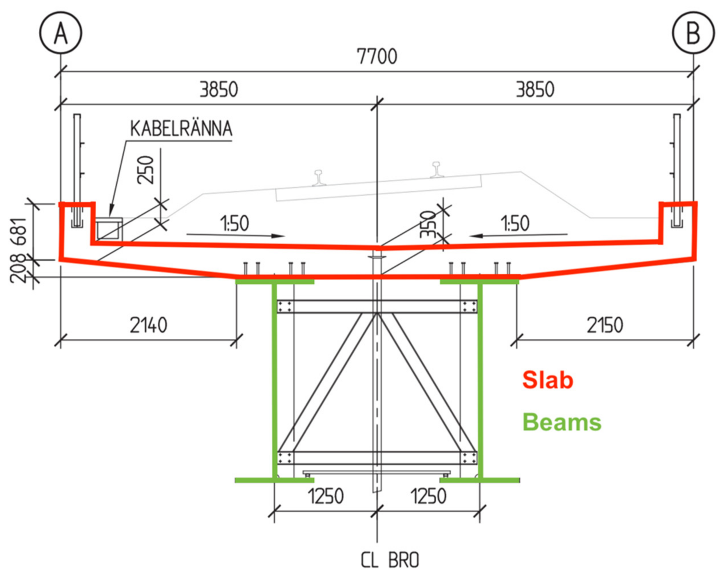
The present research work is focused on the aerodynamic behavior of steel-concrete simple girder bridges. In particular, the studied section is formed by two I-beams supporting a concrete slab (Figure 1), but the analysis was made when only one or both beams were already built before constructing the concrete slab. These bridges are usually 30–50 m long, and they are widely used in Sweden.

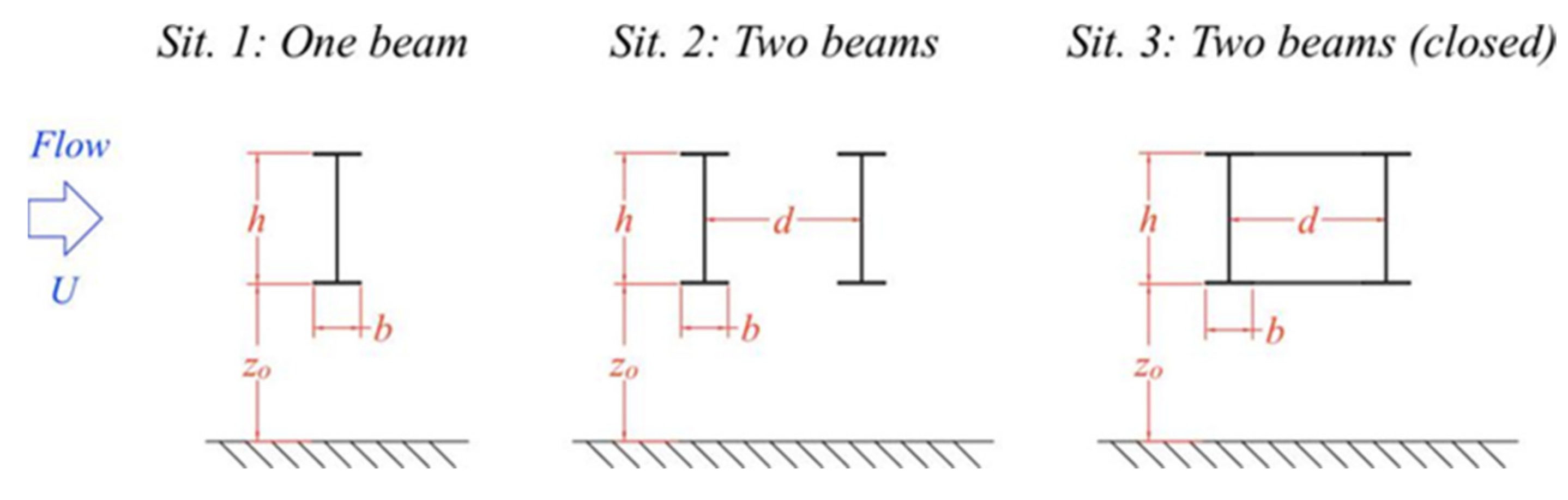
During the construction phase, both girders are placed in their final position one by one. Later, the bracing between both of them is done, and finally, the concrete slab is built. In this study, only the situations previous to the slab construction were analyzed. Therefore, the following three different case studies were considered here:

• Only one beam is installed;
• Both beams are installed;
• Both beams are installed, but the space between them is isolated from the external flow with wood or steel plates (Figure 2).

The second case covers both before and after the construction of the bracing. Therefore, the actions on the first beam, the second beam, and both beams joined were analyzed. Regarding the third situation, it was included to see if any improvement is observed in the aerodynamic parameters of the section, which would then be a possible solution to reduce its vulnerability.

During the construction of the plate, there is a period of time when the concrete is not hardened yet, and the structure does not have its final stiffness. At this stage, the added mass leads the structure to be less vulnerable to wind effects. Thus, this situation was not considered in the present study. Since the assessment was made for different construction stages, the expected winds endured by the structure are lower than in the final stage. The exposure time is in the order of days or weeks, so extreme winds are unlikely to occur during the studied situations. Vortex shedding effects are dangerous, with wind speeds between 5 and 15 m/s [25], while buffeting effects usually need much higher winds to cause large vibrations [26]. Therefore, the analysis concentrated on the vortex shedding phenomenon rather than on the bridge’s response to turbulent winds. However, the aerodynamic coefficients extracted during the study can also be applied to analytical methods to calculate the structural response to turbulence. This response is proportional to the drag coefficient, so a decrease in it would also imply a reduction in dynamic wind effects induced by turbulence.

2. Materials and Methods

2.1. Simulation Setup

The beams’ height for simple girder bridges with spans around 40 m ranged from two to three meters, so the values of h = [2, 2.5, 3] m were tested. The distance between beams is usually equal to or larger than the section’s height, so the values were taken depending on it, leaving d = h + ∆, where ∆ = [0, 0.5, 1] m. The joint procedure usually determines the flanges’ width with the concrete slab, assuming a constant value of b = 0.9 m. The bridge’s height was assumed to be z₀ = [3,5,10] m, the usual heights for this type of bridge. Moreover, an additional height of z₀ = 120 m was considered, representing the free flow. Finally, the thickness of the flanges and the web were set to t_f = 4 cm and t_w = 2 cm, respectively.

The Reynolds number falls between 6.8 × 10⁶ and 3.1 × 10⁶, depending on the case parameters. Since the tested shapes have sharp corners and the separation of the boundary layer is expected to be always in the same location, the vortex shedding around this type of section can be considered constant for this small range of Reynolds numbers [27]. To reduce computational costs, all CFD simulations in this study were conducted in two-dimensional settings. This is a valid assumption in this particular case study, as the modeled bridge has a constant cross-section area all along the bridge. In addition, two-dimensional models showed an excellent approximation to reality when representing the vortex shedding phenomenon [28]. To achieve statistically significant results, each case study was tested with five different flow speeds within the interval where vortex shedding vibrations are more likely to occur [25]: U = [5, 7.5, 10, 12.5, 15] m/s. Therefore, 420 simulations were made with 84 different geometries.

In order to consider the turbulence effect, the Re-Normalization Group (RNG) k–ε model [29] combined with enhanced wall treatment was used. RNG model was developed using Re-Normalization group theory and can be written as follows:

$$\frac{\partial (\rho k)}{\partial t}+\frac{\partial (\rho k{u}_i)}{\partial x_i}=\frac{\partial }{\partial x_j}\left[\left(\mu +\frac{{\mu }_t}{{\sigma }_k}\right)\frac{\partial k}{\partial x_j}\right]+P_k-\rho \epsilon$$

(1)

$$\frac{\partial (\rho \epsilon )}{\partial t}+\frac{\partial (\rho \epsilon u_i)}{\partial x_i}=\frac{\partial }{\partial x_j}\left[\left(\mu +\frac{{\mu }_t}{{\sigma }_{\epsilon }}\right)\frac{\partial \epsilon }{\partial x_j}\right]+C_{1\epsilon }\frac{\epsilon }{k}{P}_k-C_{2\epsilon }^{\ast }\rho \frac{{\epsilon }^2}{k}$$

(2)

where $C_{2\epsilon }^{\ast }=C_{2\epsilon }+\frac{C_{\mu }{\eta }^3\left(1-\eta /{\eta }_0\right)}{1+\beta {\eta }^3}$ with $\eta =(Sk/\epsilon )$ and $S=\sqrt{2S_{ij}{S}_{ij}}$, k is turbulence kinetic energy per unit mass and ε is turbulent dissipation rate. More details and all the constants are given by Yakhot et al. [29].

Since the wind speeds tested imply a Mach number below 0.3 (Ma = 0.015–0.044), an incompressible flow could be assumed [30]. The air density and dynamic viscosity were assigned to be ρ_a = 1.225 kg/m³ and µ = 1.7894 × 10⁻⁵ kg/ms, respectively. The second-order time domain numerical solver was used to improve accuracy, and the maximum number of iterations per time step was set at 200 to ensure convergence. The time step size and the simulation duration for each case depend on the wind speed tested, ensuring that there are around 200 time-steps per vortex shedding cycle (

Table 1. Time step and a total time of simulation used depending on the flow speed.

Wind Speed (m/s)	5	7.5	10	12.5	15
Time step (s)	0.02	0.012	0.01	0.008	0.006
Time of simulation (s)	120	72	60	48	36
Number of time steps	6000	6000	6000	6000	6000

). A steady-state simulation with sufficient iterations to ensure a satisfactory convergence was used as initial data to start the transient simulation.

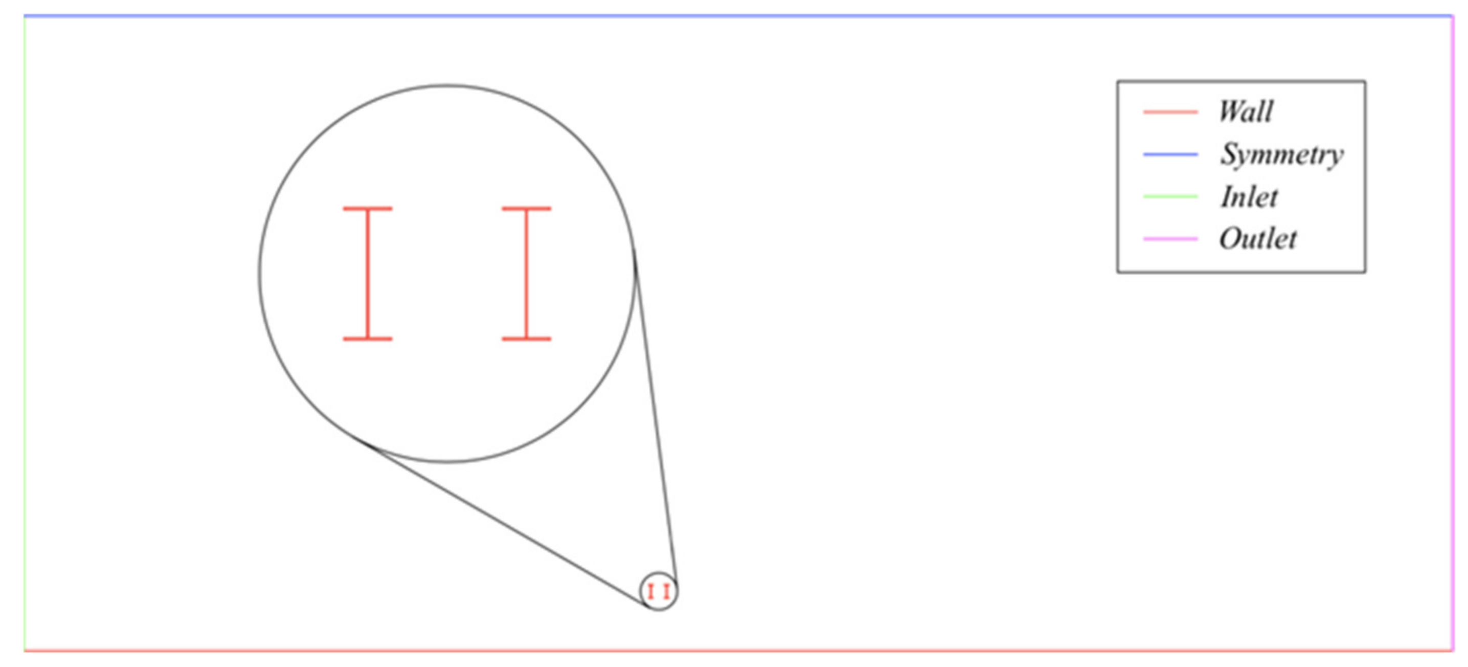
Since the case study is considered to be adiabatic, the buoyancy effect and gravitational acceleration were ignored. Wall boundary conditions with zero roughness were set for all rigid limits such as the beams and the valley. The top edge was modeled as a symmetry plane, and the left and right edges were a velocity inlet and a zero-pressure outlet, respectively. We applied symmetry boundary conditions as CAD model, and the expected pattern of the flow has mirror symmetry, as shown in Figure 3. The computational domain was extended enough to minimize the boundary conditions’ influence on the airflow prediction; namely, the inlet and the symmetry plane were moved 125 m from the beams. At the same time, the outlet was moved 150 m away from the beams (Figure 3).

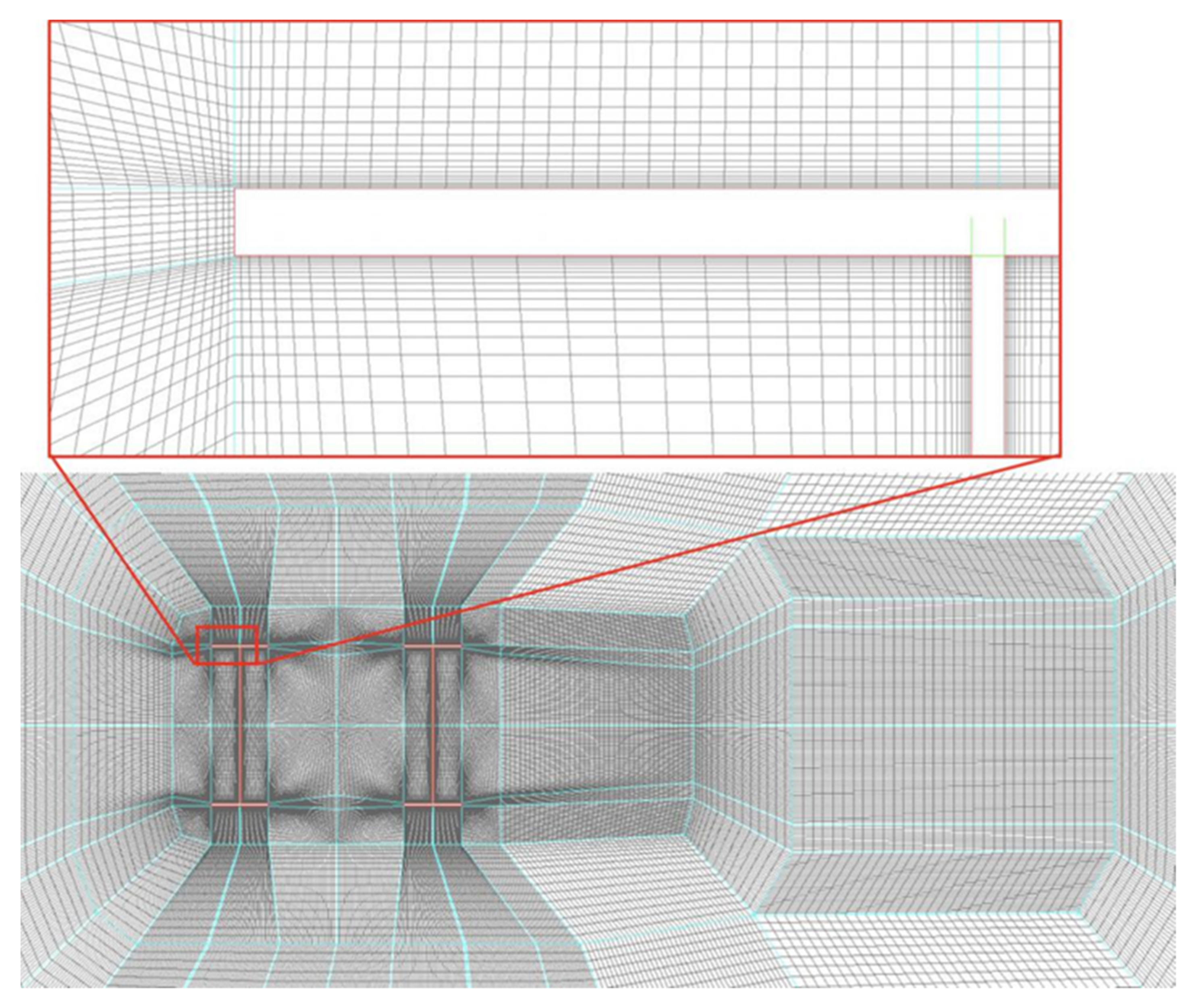
The grid generation was performed using the ICEM CFD. Local grid refinement was introduced adjacent to the beams, resulting in cells with a maximum height of 1 mm perpendicular to the surface. With a ratio of 1.2, grids were propagated throughout the computational domain (Figure 4).

From each simulation’s results, the resultant forces were calculated by integrating the pressures around all the contours of the beams, and seven time-averaged parameters were extracted: the average values of the drag, lift and moment coefficients (C_D, C_L, C_M), the corresponding Root Mean Square (RMS) values (C_D, C_L, C_M), and the Strouhal number (St). All the statistical parameters were extracted from the latter two-thirds of simulation time, where the flow was already stable. For comparison purposes, the height of the beams (h) was always taken as the reference dimension.

2.2. Model Validation

Model validation is performed through result comparisons with experimental data from the literature. Due to the lack of experimental data regarding single and double I-beams, the verification of the model was made with a similar geometry: a flat plate perpendicular to the flow. Both grid and time step convergence tests were conducted (

Table 2. Grid convergence tests were carried out for two different wind speeds of 5 m/s and 15 m/s. A mesh of 55,000 was finally chosen. Colors show the error magnitude from low (green) to high (red).

Nº Elements			42,000	55,000	68,000	81,000	94,000	107,000
Wind speed = 5 m/s	Strouhal number	Value	0.123	0.123	0.123	0.123	0.123	0.124
		Err. Prev. (%)		0	0	0	0	0.81
		Err. Final (%)	0.81	0.81	0.81	0.81	0.81
	Drag coefficient	Value	2.7131	2.7144	2.7172	2.7124	2.709	2.7102
		Err. Prev. (%)		0.05	0.1	0.18	0.13	0.04
		Err. Final (%)	0.11	0.15	0.26	0.08	0.04
	RMS Drag coefficient	Value	0.2202	0.2195	0.2212	0.2186	0.2166	0.2146
		Err. Prev. (%)		0.32	0.77	1.18	0.91	0.92
		Err. Final (%)	2.61	2.28	3.08	1.86	0.93
Wind speed = 15 m/s	Strouhal number	Value	0.121	0.121	0.121	0.122	0.122	0.122
		Err. Prev. (%)		0	0	0.83	0	0
		Err. Final (%)	0.82	0.82	0.82	0	0
	Drag coefficient	Value	2.7094	2.7139	2.7189	2.7189	0.72	2.7237
		Err. Prev. (%)		0.17	0.18	0	0.04	0.14
		Err. Final (%)	0.53	0.36	0.18	0.18	0.14
	RMS Drag coefficient	Value	0.224	0.223	0.2248	0.2213	0.2197	0.2182
		Err. Prev. (%)		0.45	0.81	1.56	0.72	0.68
		Err. Final (%)	2.66	2.2	3.02	1.42	0.69

and

Table 3. Time step test was carried out for two different wind speeds of 5 m/s and 15 m/s. 200 time-steps per cycle was finally chosen. Colors show the error magnitude from low (green) to high (red).

Approximate Time Steps per Cycle			50	100	200	400	800
Wind speed = 5 m/s	Time step size (s)		0.08	0.04	0.02	0.01	0.005
	Strouhal number	Value	0.122	0.122	0.123	0.123	0.123
		Err. Prev. (%)		0	0.82	0	0
		Err. Final (%)	0.81	0.81	0	0
	Drag coefficient	Value	2.7533	2.7356	2.7204	2.7138	2.7122
		Err. Prev. (%)		0.64	0.56	0.24	0.06
		Err. Final (%)	1.52	0.86	0.3	0.06
	RMS Drag coefficient	Value	0.2075	0.213	0.2176	0.2198	0.2207
		Err. Prev. (%)		2.66	2.16	1.01	0.41
		Err. Final (%)	5.99	3.49	1.4	0.41
Wind speed = 15 m/s	Time step size (s)		0.024	0.012	0.006	0.003	0.0015
	Strouhal number	Value	0.121	0.121	0.121	0.121	0.121
		Err. Prev. (%)		0	0	0	0
		Err. Final (%)	0	0	0	0
	Drag coefficient	Value	2.7312	2.7356	2.7204	2.7138	2.7122
		Err. Prev. (%)		0.16	0.56	0.24	0.06
		Err. Final (%)	0.7	0.86	0.3	0.06
	RMS Drag coefficient	Value	0.2134	0.2185	0.2223	0.2242	0.225
		Err. Prev. (%)		2.4	1.74	0.85	0.36
		Err. Final (%)	5.17	2.89	1.2	0.36

), and the validation was limited to the drag coefficient and the Strouhal number. The results are shown in the following tables. Err.Prev. refers to the change between a mesh and the previous one, whereas Err.Final. refers to the error with respect to the model with a greater number of elements; see Table 2 and Table 3.

Table 4. Values of the Strouhal number and drag coefficient of a flat plate normal to the flow given by [9,20,27,31] in comparison with the results obtained from the model.

	Roshko (1954)	Chen and Fang (1996)	Simiu and Scanlan (1978)	Hoerner (1992)	Model
St	0.133–0.140	0.136	0.145	-	0.121
CD	-	-	1.96–2.01	1.98	2.72

shows a comparison between the results from the model and experimental data from the published literature given by Roshko [9], Chen and Fang [20], Simiu and Scanlan [27], and Hoerner [31]. The comparison clearly shows that the drag coefficient is overestimated by 30–40%, while the Strouhal number was underestimated by 10–20%, however, the general trend was captured correctly. Considering the complexity of the problem, the domain size, and the limitations of the k–ε turbulence model, the reported deviation falls within the acceptable margin of engineering applications, and therefore, the results were considered to be valid for a qualitative analysis.

3. Results

3.1. Single Beam

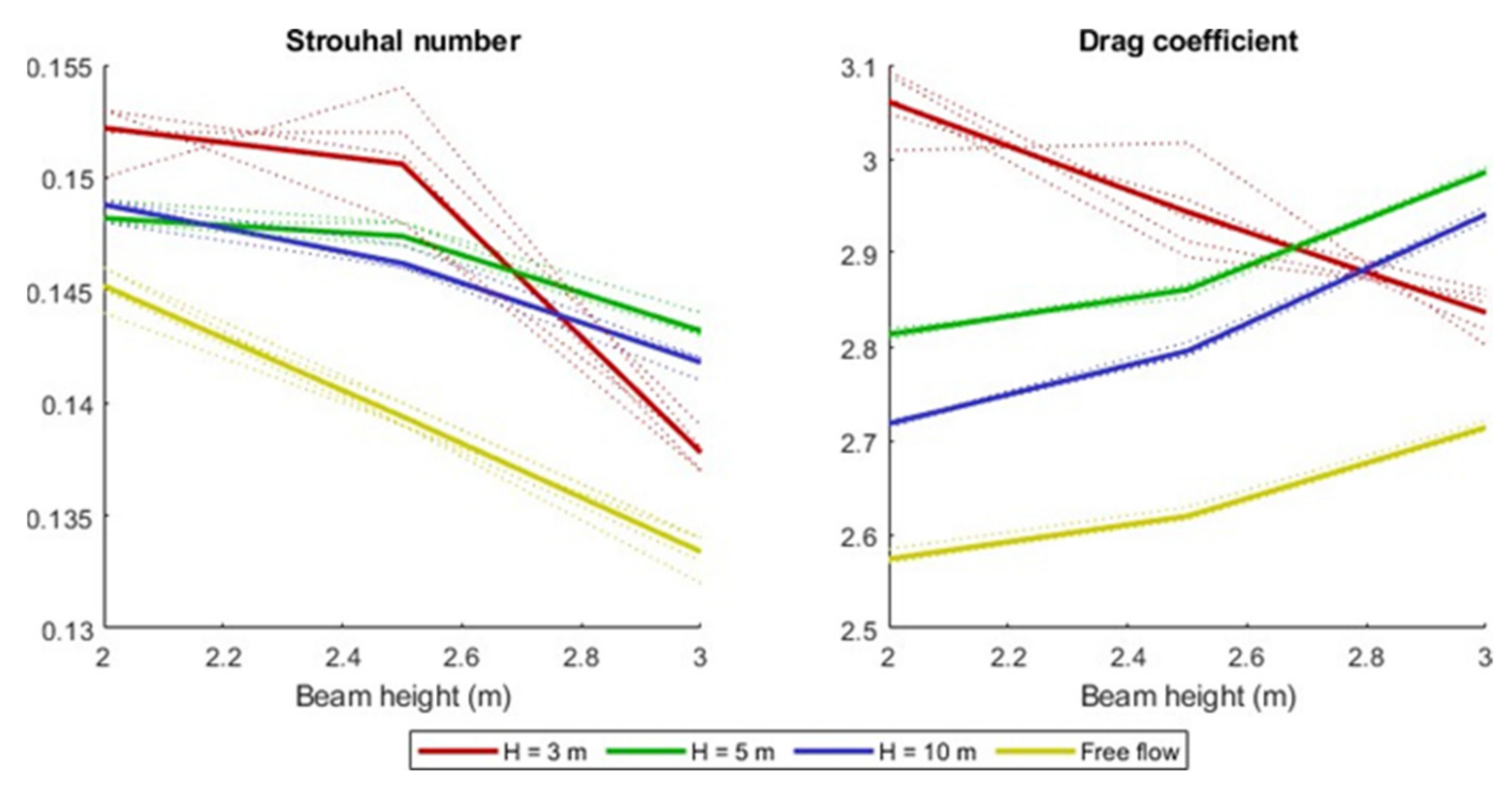
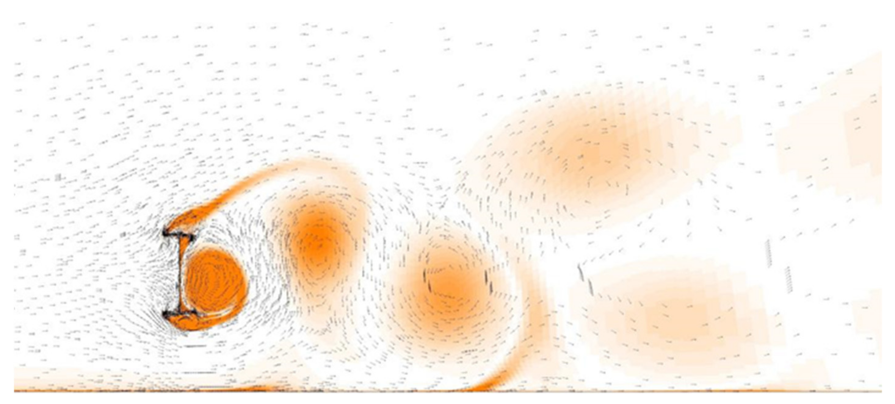
Figure 5 shows the drag coefficient and Strouhal number obtained in each simulation with a single beam geometry. Note that the simulation results of z₀ = 3 m do not follow the same path as the other simulations, and obtained aerodynamic coefficients change considerably depending on the wind speed. The influence of the proximity of the ground could explain these strange results (Figure 6). The no-slip condition in the ground is generating a small boundary layer, so the closer to it the section is, the lower the actual wind speed will be.

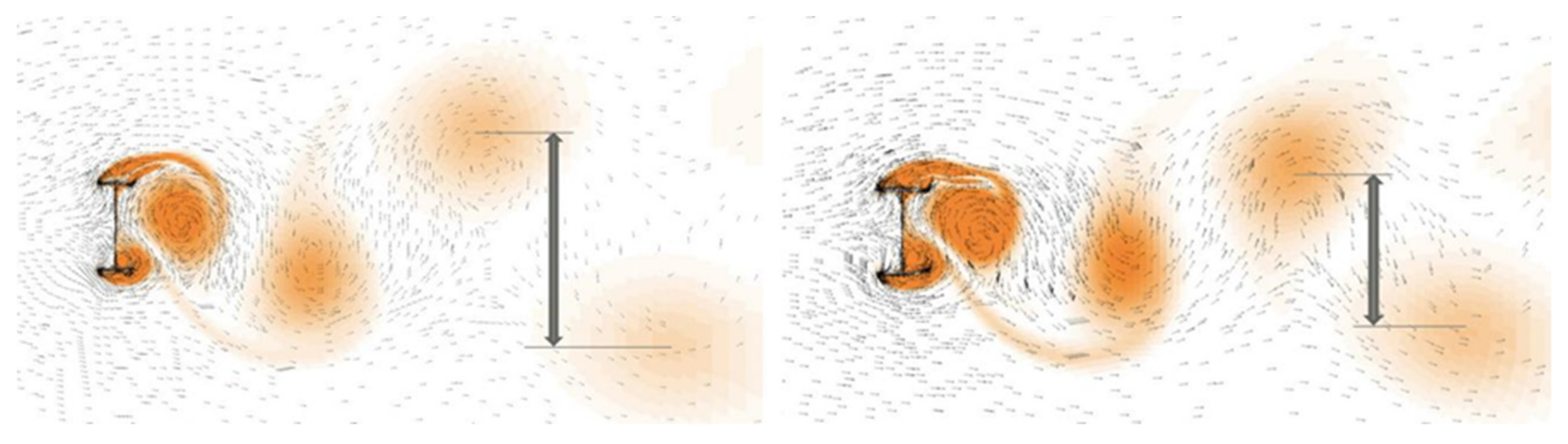
Regarding the simulations with higher bridges, some common trends can be observed. By increasing the beam height (h), the Strouhal number decreases, while the drag coefficient increases, except for H = 3 m, which might be affected by the ground boundary layer. Roshko [9] observed that the wider the wake is, the higher the drag coefficient and the lower the Strouhal number are. A considerable change in wake’s width was observed in the graphical results (Figure 7), upholding the experiments made by Roshko [9]. Since the extracted parameters are non-dimensional and depend only on the shape of the section, it can be thought that the ratio b/h is the cause of the changes in the width and the aerodynamic coefficients.

Regarding the distance to the ground, both parameters increase when the bridge becomes closer to it. The increase in both parameters is probably caused by a mechanism similar to the blockage effect, which is also observed in wind tunnel tests. Although the model has no limits on the upper side, the ground’s proximity also hinders the flow around the lower side of the section. This resistance increases the pressure in the upstream zone, increasing both parameters.

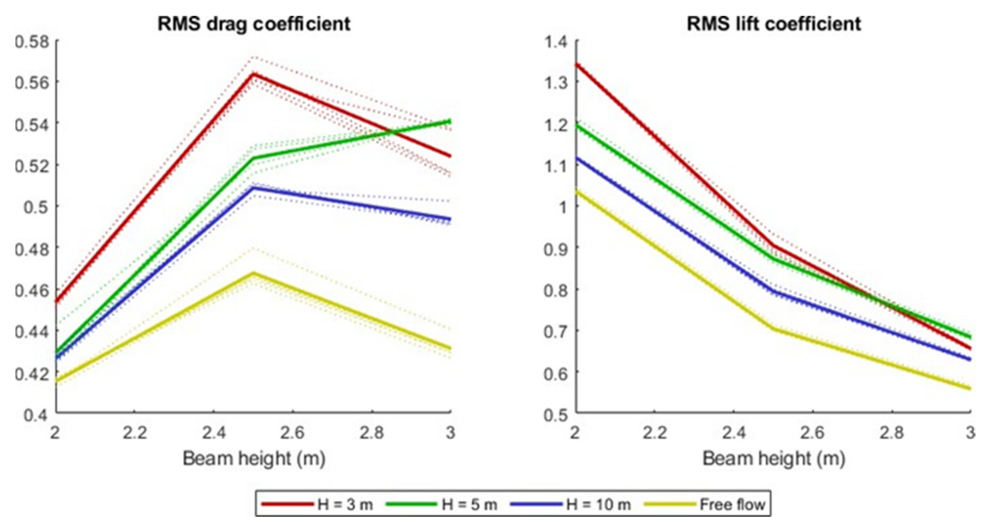
About the oscillations of the forces, the lift coefficient decreases considerably when the beam height increases (Figure 8). This result was expected, as the reference dimension for calculating the coefficients was the height of the beams. Thus, when the beam height increases, the reference dimension increases, but the flanges’ area remains the same. Regarding the drag oscillations, a peak in the intermediate values of h can be observed (Figure 8).

3.2. Double Beam

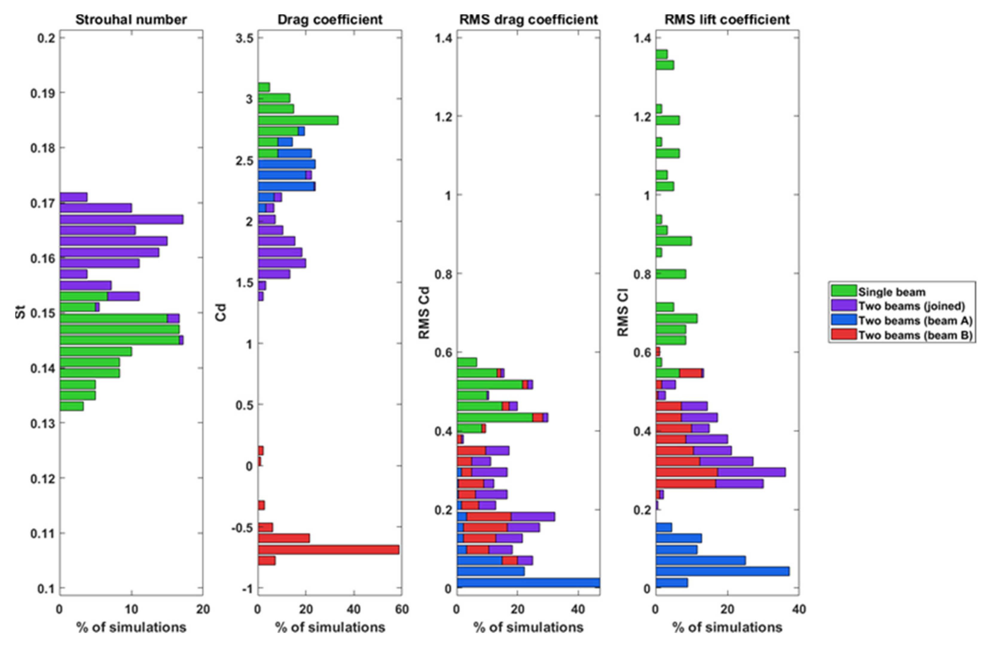
As mentioned in Section 1.2, this situation involves two structural cases: when the beams are free to move and joined by the bracing. Figure 9 shows all the results for each beam individually, and both beams joined. Each result represents a particular geometrical configuration and wind speed. Thus, the overall values obtained in each case can be observed, being possible to compare between them. The single-beam results are also included in the plot to facilitate the comparison between construction stages.

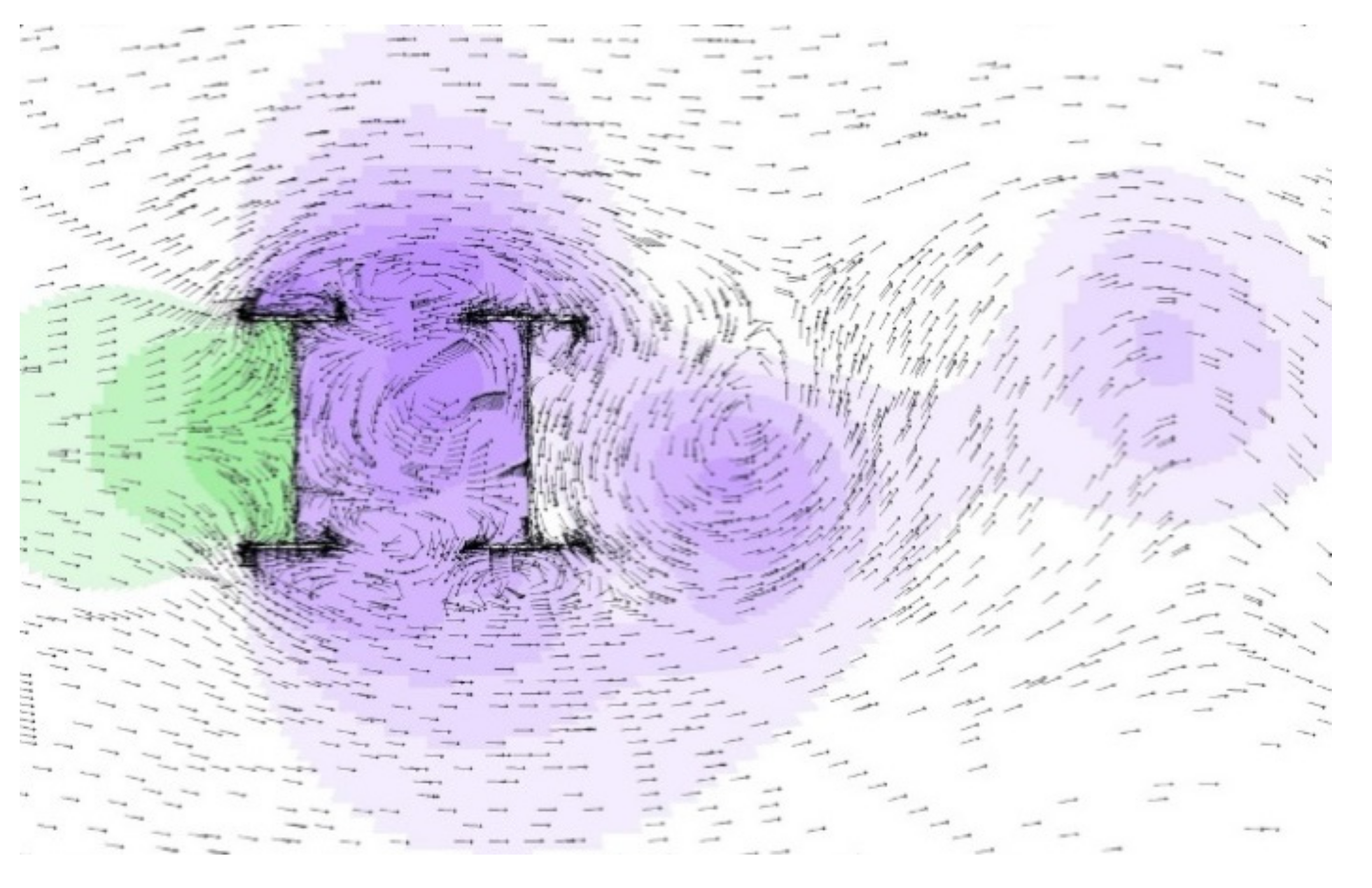
The numerical simulation predicts an increase in the Strouhal number when both beams are in their final locations. This might also mean a decrease in the wake’s width. About the actions on each beam, the upstream one has a similar drag force than in the single-beam case, while the downstream beam has only a small negative drag, see Figure 9. The recirculation zone between the beams results in a low-pressure area between the beams, which is even lower than those near the downstream of beam B.

This is expected since the pressure between both beams is slightly lower than the one in the downstream region and much lower than in the upstream region (Figure 10). Thus, the upstream beam has a large pressure difference, while the downstream beam is surrounded by flow with similar pressures. Regarding the oscillation of the forces, it can be seen that they are reduced when both beams are in their final location, especially in the case of lift oscillations. It seems that the double beam configuration changes the flow structure and reduces the dynamic airflow fluctuations.

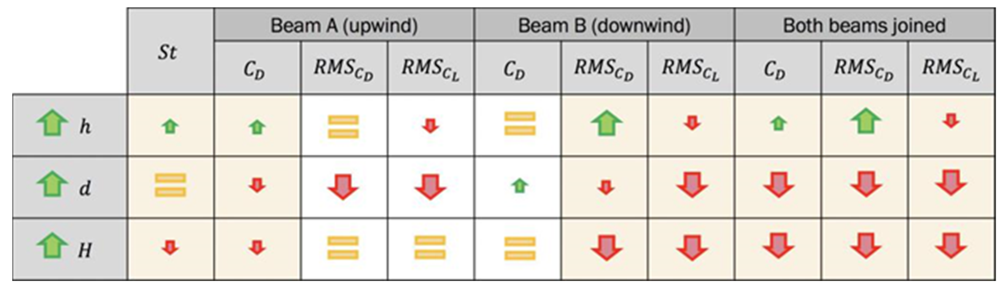
Finally, it is important to note that the along-wind dynamic effects (the ones acting in the wind direction) have amplitudes in the same order of magnitude as the cross-wind dynamic effects (the ones acting in the vertical direction). Even though cross-wind actions are usually larger, the studied section has a significant area perpendicular to the flow, increasing along-wind loads. Figure 11 summarizes the influence of the different geometric parameters on the obtained aerodynamic coefficients regarding the cross-section area changes. Due to many geometrical configurations, it is impossible to analyze each case in the present paper. To see the complete results in tabular and graphical form, with all seven parameters extracted from the 420 simulations, please see Martínez-López [32].

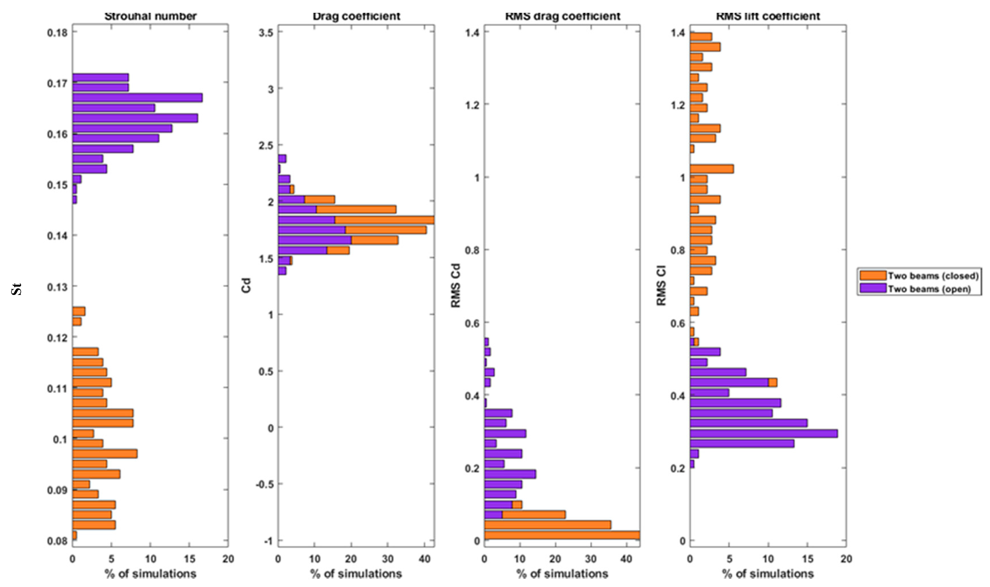
3.3. Closed Section

Figure 12 compares the results with and without slabs closing the space between beams. Even though the drag coefficient remains the same in both situations, the Strouhal number decreases by almost 50%. In addition, drag and lift oscillation amplitudes show an opposite response to the geometric modification. The RMS drag amplitudes were reduced to nearly zero values, while the RMS lift amplitudes increased to values similar to the single beam situation.

4. Discussion

The importance of long-wind vibrations produced by vortex shedding seems to be the most crucial conclusion among all achieved results. The tall and thin shape of the beam cross-section leads to significant drag dynamic effects in the same order of magnitude as lift oscillations. Considering that the bending stiffness of the beams is considerably lower in the horizontal direction, the dangerous effects are the ones in the along-wind direction. A lower stiffness implies higher amplitudes and lower frequencies of vibration, meaning more vulnerability to dynamic effects. Furthermore, the frequency of the vortex shedding loads in the along-wind direction is twice the one in the cross-wind direction. The methods proposed by Eurocode to evaluate dynamic-wind response in the along-wind direction can be applied using only the drag coefficient. However, they do not include vortex shedding loads in this direction. The methods proposed for vortex shedding evaluation only consider cross-wind vibrations. Thus, it would be necessary to study the along-wind vibrations induced by vortex shedding and adapt the analytical methods if required.

It was observed that the structural system is more vulnerable when only one beam is installed. Usually, this construction stage lasts only for a few days, so high winds’ risk is lower. Nevertheless, the wind can severely damage the bridge if the first beam is erected when the flow velocity is near the critical vortex shedding wind speed.

When both beams are mounted, there are different solutions to reduce the wind effects on the structure. First, increasing the beams’ distance is a simple solution if the project is still in the design stages. Unlike other geometrical modifications, this variation does not change the vertical bending stiffness of the bridge. Therefore, the changes could be made without redesigning the complete structure. Second, closing the section with wood or steel slabs is an effective solution to reduce wind effects before the concrete slab has been built. The Strouhal number reduction implies higher critical wind speeds with lower probabilities of occurrence. Furthermore, this solution leads to a considerable decrease in the along-wind dynamic effects caused by vortex shedding. Although cross-wind effects increase at the same time, it is rather unlikely that the low frequency of the cross-wind vortex shedding load could match the high frequency of the structure in this direction.

In general, all the simulations done describe the overall aerodynamic behavior of simple girder bridges under construction with the studied cross-section. The study highlights the potentially dangerous wind-induced actions during these bridges’ construction, and gives qualitative data to use in design stages and future research.

5. Conclusions

A comprehensive research study regarding the stability of simple girder bridges during construction stages has been performed using the Computational Fluid Dynamics technique. From the simulations done, the following qualitative conclusions could be extracted:

• For tall and thin beams like those studied in this paper, wind-induced loads are more dangerous in the along-wind direction than in the cross-wind direction.
• The most vulnerable stage is when only one beam is in its final location. Having both beams placed reduces dynamic wind loads, especially the effects induced by vortex shedding.
• An increase in the distance between beams reduces the vulnerability of the section.
• Placing non-structural wood or steel slabs to isolate the space between beams considerably reduces wind actions, especially the RMS value of the drag coefficient.

References

- Meseguer, J.; Andres, A.S.; Pindado, S.; Franchini, S.; Alonso, G. Aerodinamica Civil. In Efectos del Viento en Edificaciones y Estructuras, 2nd ed.; Ibergarceta Publicaciones, SL: Madrid, Spain, 2013. [Google Scholar]
- Davenport, A.G. The Application of Statistical Concepts to the Wind Loading of Structures; Institution of Civil Engineers: London, UK, 1961; Volume 19, pp. 449–472. [Google Scholar]
- Davenport, A.G. The Response of Slender, Line-Like Structures to a Gusty Wind; Institution of Civil Engineers: London, UK, 1962; Volume 23, pp. 389–408. [Google Scholar]
- Davenport, A.G. Gust loading factors. J. Struct. Div. 1967, 93, 11–34. [Google Scholar] [CrossRef]
- Davenport, A.G. How can we simplify and generalize wind loads? J. Wind Eng. Ind. Aerodyn. 1995, 54, 657–669. [Google Scholar] [CrossRef]
- Simiu, E. Wind spectra and dynamic alongwind response. J. Struct. Div. 1974, 100, 14. [Google Scholar] [CrossRef]
- Simiu, E. Revised procedure for estimating along-wind response. J. Struct. Div. 1980, 106, 1–10. [Google Scholar] [CrossRef]
- Dyrbye, C. , Hansen, S.O. Wind Loads on Structures; Wiley (John) & Sons, Limited: Chichester, UK, 1997. [Google Scholar]
- Roshko, A. On the drag and shedding frequency of two-dimensional bluff bodies. In Dynamische Windwirkung an Bauwerken; Ruscheweyh, H., Ed.; Wiesbaden: Berlin/Bauverlag, Germany, 1954. [Google Scholar]
- Ruscheweyh, H. Further studies of wind-induced vibrations of grouped stacks. J. Wind Eng. Ind. Aerodyn. 1983, 11, 359–364. [Google Scholar] [CrossRef]
- Vickery, B.J.; Clark, A.W. Lift or across-wind response to tapered stacks. J. Struct. Div. 1972, 98, 1–20. [Google Scholar] [CrossRef]
- Vickery, B.J. A model for the prediction of the response of chimneys to vortex shedding. In Proceedings of the 3rd International Symposium Design of Industrial Chimneys, Munich, Germany, 1978; pp. 157–162. [Google Scholar]
- Vickery, B.J.; Basu, R.I. Across-wind vibrations of structures of circular cross-section. part i. development of a mathematical model for two-dimensional conditions. J. Wind Eng. Ind. Aerodyn. 1983, 12, 49–73. [Google Scholar] [CrossRef]
- Vickery, B.J.; Basu, R.I. Across-wind vibrations of structures of circular cross-section. part ii. development of a mathematical model for full-scale application. J. Wind Eng. Ind. Aerodyn. 1983, 12, 75–97. [Google Scholar] [CrossRef]
- Vickery, B.J.; Basu, R.I. Simplified approaches to the evaluation of the across-wind response of chimneys. J. Wind Eng. Ind. Aerodyn. 1983, 14, 153–166. [Google Scholar] [CrossRef]
- Solari, G. Progress and prospects in gust-excited vibrations of structures. Engng Mech 1999, 6, 301–322. [Google Scholar]
- Giosan, I.; Eng, P. Vortex Shedding Induced Loads on Free Standing Structures. In Structural Vortex Shedding Response Estimation Methodology and Finite Element Simulation; 2013; Volume 42, Available online: http://citeseerx.ist.psu.edu/viewdoc/summary?doi=10.1.1.582.3179 (accessed on 9 June 2021).
- Eurocode 1. Actions on Structures. Part. 1–4: General Actions—Wind Actions. 2005. Available online: https://en.wikipedia.org/wiki/Eurocode_1:_Actions_on_structures#Part_1-4:_General_actions_-_Wind_actions (accessed on 9 June 2021).
- NBC. National Building Code of Canada 2015; NBC: New York, NY, USA, 2015. [Google Scholar]
- Chen, J.M.; Fang, Y.C. Strouhal numbers of inclined flat plates. J. Wind Eng. Ind. Aerodyn. 1996, 61, 99–112. [Google Scholar] [CrossRef]
- Radi, A.; Thompson, M.C.; Sheridan, J.; Hourigan, K. From the circular cylinder to the flat plate wake: The variation of strouhal number with reynolds number for elliptical cylinders. Phys. Fluids 2013, 25, 101706. [Google Scholar] [CrossRef]
- Lam, K.; Wei, C. Numerical simulation of vortex shedding from an inclined flat plate. Eng. Appl. Comput. Fluid Mech. 2010, 4, 569–579. [Google Scholar]
- Consolazio, G.R. , Gurley, K.R., Harper, Z.S. Bridge Girder Drag Coefficients and Wind-Related Bracing Recommendations; Technical Report; University of Florida: Gainesville, FL, USA, 2013. [Google Scholar]
- Gandia, F.; Meseguer, J.; Sanz, A. Influence of aerodynamic characteristics of “H” beams on galloping stability. In Proceedings of the 37th IABSE Symposium: Engineering for Progress, Nature and People, Madrid, Spain, 3–5 September 2014; pp. 277–284. [Google Scholar]
- Dexter, R.; Ricker, M. Fatigue-Resistant Design of Cantilevered Signal, Sign, and Light Supports; Nchrp Report 469; Transportation Research Board of the National Academies: Washington, DC, USA, 2002. [Google Scholar]
- Strømmen, E. Theory of Bridge Aerodynamics; Springer Science & Business Media: Berlin/Heidelberg, Germany, 2010. [Google Scholar]
- Simiu, E.; Scanlan, R.H. Wind Effects on Structures; Wiley: Hoboken, NJ, USA, 1978. [Google Scholar]
- Mureithi, N.W.; Xu, X.; Baranyi, L.; Nakamura, T.; Kaneko, S. Dynamics of the forced karman wake: Comparison of 2d and 3d models. In Proceedings of the ASME 2014 Pressure Vessels and Piping Conference, Anaheim, CA, USA, 20–24 July 2014. [Google Scholar]
- Yakhot, V.; Orszag, S.A.; Thangam, S.; Gatski, T.B.; Speziale, C. Development of turbulence models for shear flows by a double expansion technique. Phys. Fluids A Fluid Dyn. 1992, 4, 1510–1520. [Google Scholar] [CrossRef] [Green Version]
- Anderson, J.D., Jr. Fundamentals of Aerodynamics; Tata McGraw-Hill Education: New York, NY, USA, 2010. [Google Scholar]
- Hoerner, S.F. Fluid-Dynamic Drag: Theoretical, Experimental and Statistical Information; Hoerner Fluid Dynamics: Vancouver, BC, Canada, 1992. [Google Scholar]
- Martínez-López, G. Wind Effects on Simple Girder Bridges during Construction Stages. 2019. Available online: http://urn.kb.se/resolve?urn=urn:nbn:se:kth:diva-254342 (accessed on 9 June 2021).
Figure 1.
Cross-section of the Banafjäl Bridge, a railway structure of the Bothnia Line in Sweden. The bridge shows a typical simple girder bridge cross-section with two girders. Source: Royal Institute of Technology (single column, B&W in the printed version).
Figure 2.
Construction stages considered in the parametric study (single or double column, B&W in the printed version).
Figure 3.
View of the complete fluid domain, with the boundary conditions used. In the case studies with z0 = 120 m, the bottom edge was also set as a symmetry boundary condition (single or double column, B&W in the printed version).
Figure 4.
Mesh structure in the surroundings of the structure for a case with two beams (double column, B&W in the printed version).
Figure 5.
Values of the Strouhal number and drag coefficient extracted from the simulations with one beam. The dotted lines represent the results for a particular wind speed, while the continuous lines are the average values from all the wind speeds (double column, B&W in the printed version).
Figure 6.
Vorticity contour for a particular moment of the simulation with h = 3 m, b = 0.9 m, z0 = 3 m, and U = 5 m/s (double column, B&W in the printed version).
Figure 7.
Vorticity contour at a particular moment of the single beam simulations in free flow, with h = 3 m (left) and h = 2 m (right). The change in wake’s width concerning the beam height can be observed (double column, B&W in the printed version).
Figure 8.
Root Mean Square (RMS) values of the drag and lift coefficients extracted from the simulations with one beam. The dotted lines represent the results for a particular wind speed, while the continuous lines are the average values from all the wind speeds (double column, B&W in the printed version).
Figure 9.
Distribution of the Strouhal number, the drag coefficient, and RMS values of the drag and lift coefficients for the different situations and structural configurations. Beam A represents the upstream beam, while Beam B represents the downstream beam (double column, B&W in the printed version).
Figure 10.
Pressure field for a simulation with two beams. Purple low-pressure zones and green represent high-pressure zones.
Figure 11.
Influence of the variations of each geometrical parameter on the aerodynamic coefficients of the section. Small arrows represent maximum changes around 5–10%, while large arrows represent maximum changes of more than 10%. Cells with white background represent parameters with nearly zero values.
Figure 12.
Distribution of the Strouhal number, drag coefficient, and Root Mean Square values of the drag and lift coefficients with and without the wooden/steel slabs isolating the space between beams (double column, B&W in the printed version).