A New Method for Evaluating the Bearing Capacity of the Bridge Pile Socketed in the Soft Rock

Abstract

Aiming at the rock-socketed pile in the soft rock area, this paper studies the inherent constitutive relationship between the vertical restraint stiffness at the pier bottom and the bearing capacity of the pile foundation. A new method to evaluate the bearing capacity of the pile foundation is proposed. Based on the Rayleigh energy method and the Southwell frequency synthesis method, the analytical expression of the vertical vibration fundamental frequency of the pier was calculated, and the constraint stiffness expression of the pier bottom was derived. By investigating the impact of parameters on the bearing capacity coefficient of the pile foundation, the fitting formula of the bearing capacity coefficient was obtained by multiple linear regression. Then, with this method, the vertical fundamental frequency of the pier was obtained through a field dynamic test to calculate the vertical constraint stiffness and evaluate the bearing capacity of the rock-socketed pile in the soft rock area. This method can overcome the shortcomings of the traditional static load test method, such as the high cost, long cycle, and poor representativeness. Finally, this method’s accuracy was verified by comparing field measurements and finite element simulation results. The results show that the difference between the code design constraint stiffness and the constraint stiffness by the frequency synthesis method was about 0.7%, and the bearing capacity difference between the analytical solution and the numerical simulation was small. The new method is accurate and effective.

1. Introduction

The distribution of rock strata in China is mainly soft rock; therefore, the rock-socketed pile foundation is embedded mostly on soft rock. Researchers [1,2,3,4,5,6] have investigated and measured the properties of soft rock with different methods. According to engineering data, as Gannon et al. [7] pointed out, the uniaxial compressive strength of soft rock is between $0.6\mathrm{and}12.5\mathrm{MPa},$ and the modulus is between $100\mathrm{and}100000\mathrm{MPa}$.

Researchers have also carried out many studies on the vertical bearing properties of socketed piles in soft rock. Based on the analysis of 14 groups’ static load test results of rock-socketed piles, McVay et al. [8] established a relationship between the unconfined compressive strength, splitting strength of limestone, and pile side friction. With the dilatancy effect and the slip-line field theory, Zhang et al. [9] studied the shear failure process of the vertically loaded bearing pile socketed into weak rocks. Singh et al. [10] performed a parametric analysis on the rock-socketed pier and revealed the impact of these parameters on the pier behaviors. Hassan et al. [11] carried out an in-situ static load test and a numerical calculation analysis on both deep and shallow rock-socketed piles embedded in argillaceous rock at the pile end and put forward a formula for the bearing capacity of rock-socketed piles. Zhao et al. [12] conducted a vertical static load test on rock-socketed piles embedded in muddy siltstone. The results showed that the load settlement curve of ultra-long rock-socketed piles falls slowly, and there is no significant turning point. Zhao also established the shear function based on the shear failure and dilatancy effect and determined the relationship between the embedded depth and section roughness [13]. By considering the elastic and elastic-visco-plastic properties of the surrounding and underlying soils, Ter-Martirosyan et al. [14] presented a method for determining an incompressible pile’s settlement and bearing capacity. Cai et al. [15] investigated the bearing mechanism of rock-inclined piles and proposed an efficient method to estimate the bearing capacity of the piles.

Due to the large bearing capacity and high cost of a static load test of the rock-socketed pile in weak rock, almost no destructive tests have been carried out in engineering applications. Therefore, the research on the bearing properties of rock-socketed piles in the soft rock area is mainly based on modeling tests. The vertical bearing capacity of rock-socketed piles is generally obtained by numerical simulation and field test piles measured data [16,17,18]. Huang et al. [19] conducted indoor model tests of rock-socketed piles in the soft rock under different overburden pressures and socketed depths, investigated the piles’ axial bearing characteristics, and revealed the bearing mechanism and influencing factors. To obtain the natural frequency calculation of structures, researchers [20,21,22,23] have investigated different methods. The frequency synthesis method is an effective way to establish the relationship between the natural frequency and the constraint stiffness. With the frequency synthesis method, An and Li deduced the natural frequency of the variable cross-section pier, considering the support spring constraint and proposed the analytical algorithm of the transverse vibration frequency of the column pier [24]. Feng et al. studied the bridge pile foundation vertical capacities based on numerical simulation and indoor model tests, analyzed the relationship between the position of the pile and the resistance of the pile side and the bearing capacity of the pile foundation, and proposed a more accurate indoor pile foundation test method [25]. Gao et al. carried out a series of field loading tests of 16 large-diameter belled concrete piles and discussed the influence of pile dimensions on vertical bearing capacity [26].

At present, the most convincing method to determine the bearing capacity of bridge pile foundation is the field static load test. However, this method has a long test cycle with a high cost, a sophisticated test process, and specific loading conditions for the test field. In addition, due to the complex geological conditions in mountainous areas, few pile foundation test results are not representative. This has become another inevitable problem of bridge pile foundations in mountainous regions. Therefore, to ensure the safety of structures and bring economic benefits, it is necessary to present a method to reduce the test cost and evaluate the bearing capacity of the pile conveniently.

In this paper, a new method to evaluate the bearing capacity of the pile foundation by dynamic testing is presented. The bearing capacity of the pile foundation can be calculated theoretically only by identifying the vertical fundamental frequency of bridge piers. This method is simple, quick, and low-cost. First, based on the Rayleigh energy method and frequency synthesis method, the analytical expression of the constraint stiffness of the pier bottom is derived. Then, the bearing capacity coefficient (i.e., the bearing capacity and stiffness constraints both constitutive) with six types of influence factors are introduced and analyzed. With a convenient dynamic field test of the pier, the vertical fundamental frequency of the pier can be observed, and the constraint stiffness of the pile foundation can be identified with the frequency. Last, the vertical bearing capacity of the pile foundation is evaluated by the fitted bearing capacity coefficient and verified by the finite element method.

2. Research Methodology

2.1. The Calculation Method of the Vertical Fundamental Frequency of Bridge Piers

The multi-component complex system consists of the mass element and the deformation element. The mass element is the mass state of each part of the system, and the deformation element is the deformation state of each part of the system. Each mass element and deformation element can be combined as a single subsystem, and its fundamental frequency can be calculated by the Rayleigh energy method. Then, the fundamental frequency of the whole multi-component complex system is synthesized by the frequency synthesis method. As the natural frequency calculated by the energy method is the upper-limit value of the fundamental frequency, the frequency calculated by the combination of the Rayleigh energy method and frequency synthesis method may not necessarily be the lower-limit solution. However, according to practical applications, this method is considered accurate in calculating the spatial fundamental frequency of bridge piers.

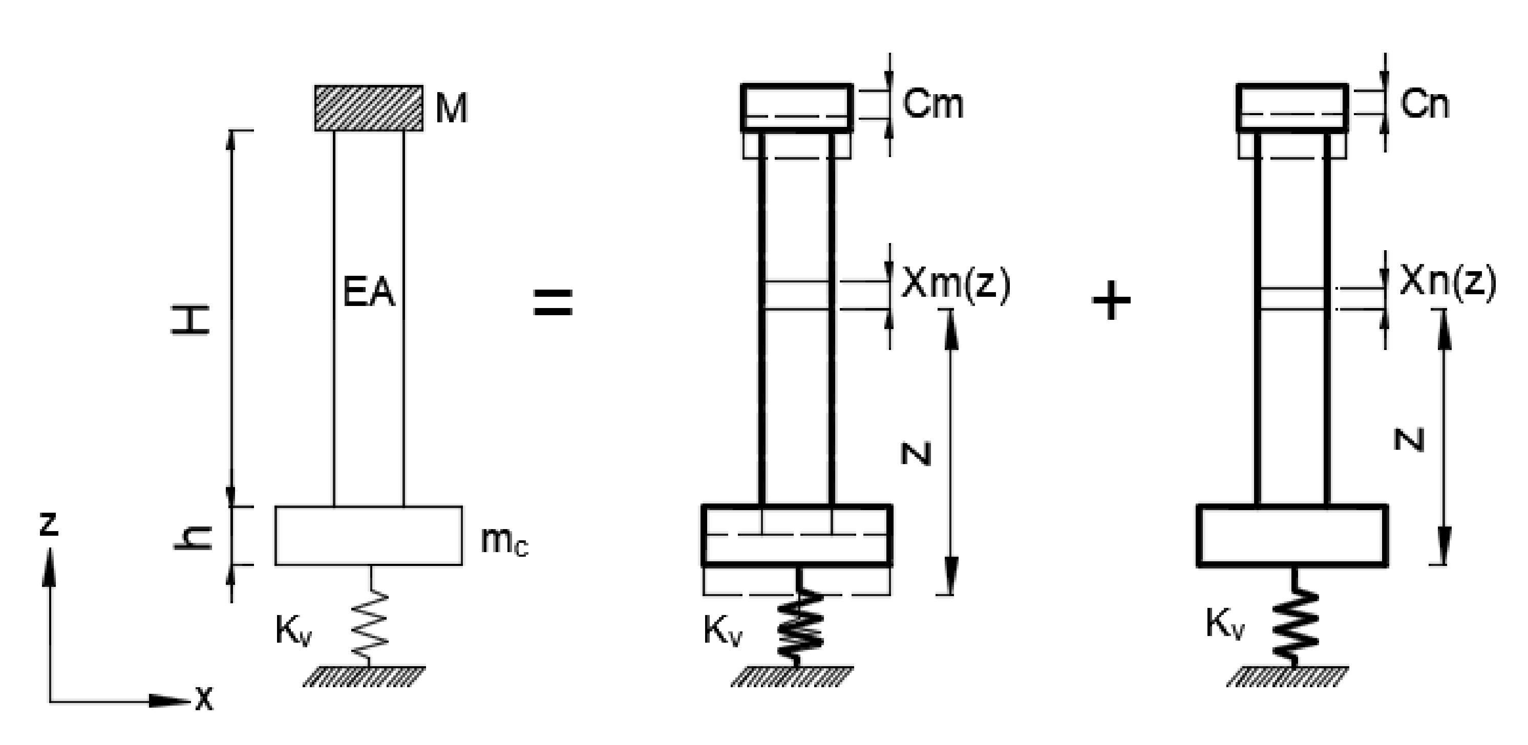
Because of the pile side resistance, the pile end resistance, and the compressive capability of concrete, the pile foundation has vertical stiffness. The stiffness also acts on the pier bottom and gives the pier bottom a specific vertical restraint stiffness $K_v$. In the condition of the bare pier, the constraint stiffness can be expressed by vertical translational spring, and the top of the pier is unconstrained. As shown in Figure 1, the pier displacement caused by vertical vibration consists of two parts: the pier’s vertical translation $x_m\left(z\right)$ and the pier’s vertical deformation $x_n\left(z\right)$. The vertical translation amplitude and the vertical deformation amplitude of the pier are expressed as $c_m$ and $c_n$, respectively.

As the mass and stiffness of piers are continuously distributed, it will result in low accuracy when calculated by the discrete multi-degree-of-freedom method. The Hamilton principle is used to derive the vibration shape function of the pier with infinite degrees of freedom. As shown in Figure 1, $H$ is the pier height, $m$ is the continuous mass, $EA$ is the vertical stiffness, $M$ is the mass at the pier top, $m_c$ is the mass of the platform, and the $h$ is the height of the platform. With the vertical vibration caused by the distributed load on the pier top, the vertical displacement on the central axis of the pier is expressed as $u\left(z,t\right)$. The initial position under the self-weight of the pier is the equilibrium position. The kinetic energy $T$ and the potential energy $V$ of vertical vibration of the pier are expressed as:

$$T=\frac{1}{2}{{\displaystyle \int }}_0^{H}m{\left(\frac{\partial u}{\partial t}\right)}^{2}dz$$

(1)

$$V=\frac{1}{2}{{\displaystyle \int }}_0^{H}EA{\left(\frac{\partial u}{\partial z}\right)}^{2}dz$$

(2)

Without considering the work done by an external load, according to Hamilton’s principle, there is an equation defined as:

$${{\displaystyle \int }}_{t1}^{t2}\delta \left(T-V\right)dt=0$$

(3)

where $t1, t2$are any two moments.

Introducing Equations (1) and (2) into (3) gives the equation:

$${{\displaystyle \int }}_{t1}^{t2}{{\displaystyle \int }}_0^h\left[EA\frac{{\partial }^{2}u}{\partial t^2}-m\frac{{\partial }^{2}u}{\partial z^2}\right]\delta udzdt=0$$

(4)

For any $\delta u$, Equation (4) can be expressed as the bridge pier’s partial differential equation of vertical vibration.

$$m\frac{{\partial }^{2}u}{\partial t^2}-EA\frac{{\partial }^{2}u}{\partial z^2}=0$$

(5)

In $u\left(z,t\right)=\phi \left(z\right)q\left(t\right)$, $\phi \left(z\right)$ is the vertical vibration shape function, and $q\left(t\right)$ is the primary coordinate function, which represents the vibration amplitude of the vertical pier vibration. Substituting $u\left(z,t\right)$ into Equation (5) and using the separating variables method gives the following equation:

$$\frac{EA\phi {(z)}^{″}}{m\phi \left(z\right)}=\frac{\ddot{q}\left(t\right)}{q\left(t\right)}$$

(6)

The left side of Equation (6) is a function of the coordinate $z$, and the right side is a function of time $t$. If Equation (6) holds for any $z$ and $t$, they must be equal to the same constant. Supposing that the constant is $a$, then:

$$\phi {\left(z\right)}^{”}-\frac{am}{EA}\phi \left(z\right)=0$$

(7)

$$\ddot{q}\left(t\right)-aq\left(t\right)=0$$

(8)

Only when the constant $a$ is negative can the vertical vibration Equations (7) and (8) of the bridge pier be solved. Setting the constants $a=-{\omega }^2,{\beta }^2={\omega }^2\frac{m}{EA}$ yields the following equations:

$$\phi \left(z\right)=A\mathit{sin}\beta x+B\mathit{cos}\beta x$$

(9)

$$q\left(t\right)=C\mathit{sin}\omega t+D\mathit{cos}\omega t$$

(10)

The vertical vibration shape function of the pier is a trigonometric function, and its integral constants $A$ and $B$ are determined by boundary conditions. The maximum kinetic energy and potential energy of the vertical vibration of the pier are calculated with Equations (11) and (12), respectively.

$${\omega }^2\overline{T}=\frac{n}{2}{{\displaystyle \int }}_0^{H}m\left(z\right)\left[x_m\left(z\right)+x_n\left(z\right){]}^{2}dz+\frac{{\omega }^2}{2}\right[M{x}_M^2\left(z\right)+m_c{x}_m^2\left(z\right)]$$

(11)

$$\overline{V}=\frac{1}{2}{K}_v{c}_m^2+\frac{n}{2}{{\displaystyle \int }}_0^{H}EA\left(z\right){\left(\frac{\partial x_n\left(z\right)}{dz}\right)}^{2}dz$$

(12)

In these equations, $n$ is the number of piers, $x_M\left(z\right)$ is the vertical translation caused by the pier top mass, and $x_m\left(z\right)$ is the vertical translation caused by the pier body.

According to the law of conservation of energy, $T_{max}=V_{max}={\omega }^2\overline{T}=\overline{V}$. Therefore,

$${\omega }^2=\frac{\overline{V}}{\overline{T}}$$

(13)

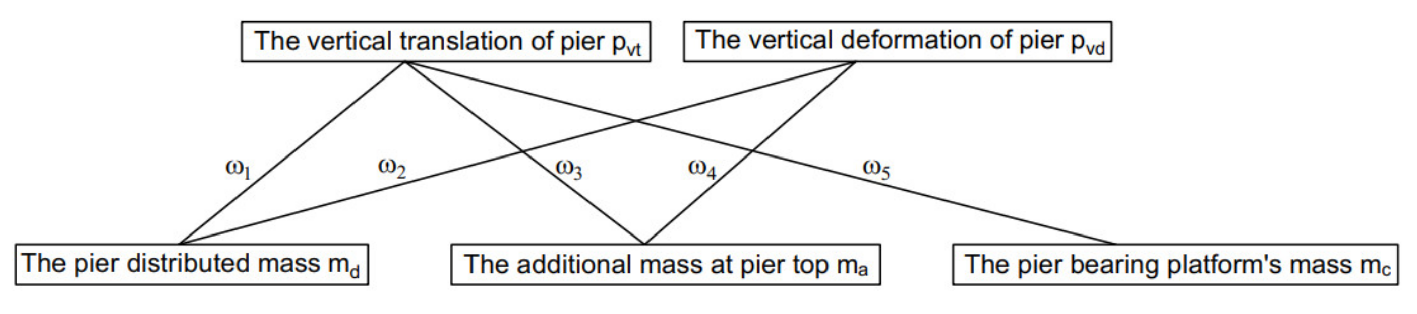
Based on the Southwell frequency synthesis method [22], the vertical mass elements and displacement elements are combined as shown in Figure 2, and the vertical fundamental frequency of the pier is:

$$\frac{1}{{\omega }_v^2}\le \frac{1}{{\omega }_1^2}+\frac{1}{{\omega }_2^2}+\frac{1}{{\omega }_3^2}+\frac{1}{{\omega }_4^2}+\frac{1}{{\omega }_5^2}$$

(14)

where ${\omega }_1$ is the fundamental frequency formed by the combination of the pier distributed mass $m_d$and the vertical pier translation $p_{vt}$, ${\omega }_2$ is the fundamental frequency formed by the combination of $m_d$ and the vertical deformation $p_{vd}$, ${\omega }_3$ is the combination of the additional mass at the pier top $m_a$ and $p_{vt}$, ${\omega }_4$ is the combination of $m_a$ and $p_{vd}$, and ${\omega }_5$ is the combination of the pier cap’s mass $m_c$ and $p_{vt}$.

According to the Rayleigh energy method, the shape function of vertical pier vibration should meet the geometric boundary conditions. The following shape equation is used for the vertical vibration of the pier system:

$$x_m\left(z\right)=c_m$$

(15)

$$x_n\left(z\right)=c_n\mathit{sin}\frac{\pi z}{2H}$$

(16)

Then, the vertical fundamental frequencies ${\omega }_1, {\omega }_2, {\omega }_3,{\omega }_4, {\omega }_5$ of each combined subsystem is calculated as:

$${\omega }_1^2=\frac{K_v{c}_m^2}{n{{\displaystyle \int }}_0^H\rho A{x}_m^2\left(z\right)dz}=\frac{K_v}{n\rho AH}$$

(17)

$${\omega }_2^2=\frac{n{{\displaystyle \int }}_0^{H}EA{\left(\frac{\partial x_n\left(z\right)}{\partial z}\right)}^{2}dz}{n{{\displaystyle \int }}_0^H\rho A{x}_n^2\left(z\right)dz}=\frac{{\pi }^{2}E}{4\rho H^2}$$

(18)

$${\omega }_3^2=\frac{K_v{c}_m^2}{M{x}_m^2\left(z\right){|}_{z=H}}=\frac{K_v}{M}$$

(19)

$${\omega }_4^2=\frac{n{{\displaystyle \int }}_0^{H}EA{\left(\frac{\partial x_n\left(z\right)}{\partial z}\right)}^{2}dz}{M{x}_n^2\left(z\right){|}_{z=H}}=\frac{n{\pi }^{2}EA}{8MH}$$

(20)

$${\omega }_5^2=\frac{K_v{c}_m^2}{m_c{c}_m^2}=\frac{K_v}{m_c}$$

(21)

Setting $m_d=n\rho AH$, the fundamental frequency of the whole system is expressed as Equation (22) by the frequency synthesis method.

$$\frac{1}{{\omega }_v^2}=\frac{M+m_d+m_c}{K_v}+\frac{\left(4m_d+8M\right)H}{n{\pi }^{2}EA}$$

(22)

In this equation, $\rho$ is the density of pier; A is the cross-section area of piers; $K_v$ is the vertical restraint stiffness of pile foundation to pier bottom (unit: $N/m$); $M, m_d, \mathrm{and} m_c$ are the masses of the pier top, pier, and pier cap, respectively; $H$ is the height of the pier; ${\omega }_v$ is the vertical fundamental frequency of the pier, $EA$ is the vertical stiffness of the pier, and $n$ is the number of the pier.

2.2. Identification of the Pier Bottom Vertical Constraint Stiffness

The fundamental frequency can be expressed as an explicit expression of the pier bottom constraint stiffness. With other parameters remaining unchanged, a specific constraint stiffness corresponds to a unique fundamental frequency, which means that a specific fundamental frequency also corresponds to a unique constraint stiffness. Therefore, the analytical equation of vertical restraint stiffness of the pier bottom expressed by fundamental frequency is:

$$K_v=\frac{M+m_d+m_c}{\frac{1}{{\omega }_v^2}-\frac{\left(4m_d+8M\right)H}{n{\pi }^{2}EA}}$$

(23)

Equation (23) can be used to predict the vertical restraint stiffness of a solid pier with an equal cross-section.

2.3. Calculation of the Pile Bearing Capacity

Referring to the design code (JTG 3363-2019), the calculation formulas of the characteristic value of the single pile vertical bearing capacity $R_a$ and the vertical constraint stiffness of the pile $K_{vs}$ are shown in Equations (24) and (25),

$$R_a=c_1{A}_p{f}_{rk}+u{\displaystyle \sum }_{i=1}^m{c}_{2i}{h}_i{f}_{rki}+\frac{1}{2}{\varsigma }_{s}u{\displaystyle \sum }_{i=1}^n{l}_i{q}_{ik}$$

(24)

where $c_1\mathrm{and}{c}_{2i}$ are the end resistance exertion coefficient and the lateral resistance exertion coefficient of the rock stratum $i$; $A_p$ is the cross-section area of the pile end (unit: m²); $f_{rk}$ is the standard value of the saturated uniaxial compressive strength of the rock at the pile end, $f_{rki}$ is the saturated uniaxial compressive strength of the rock stratum $i$, and $q_{ik}$ is the standard lateral resistance value of the soil layer $i$ at the pile side (unit: $\mathrm{KPa}$); $u$ is the circumference of the pile section and $h_i$ is the length of the pile embedded in the rock stratum $i$ (unit: $m$); $m$ is the number of rock strata and $n$ is the number of soil layers; ${\varsigma }_s$ is the lateral resistance exertion coefficient of the covered soil layer; and $l_i$ is the thickness of the rock and soil layers under the cap bottom or the partial erosion line.

$$K_{vs}=\frac{1}{\frac{l_0+\xi h}{EA}+\frac{1}{C_0{A}_0}}$$

(25)

where $\xi$ is a coefficient for the end bearing pile, $\xi =1$; $l_0$ is the free length of the pile and $h$ is the length of the pile between the bedrock and soil surface (unit: m); $A$ is the average section area of the pile in the soil; $C_0$ is the resistance coefficient of the rock foundation; $\overline{\phi }$ is the average internal friction angle of the soil layer; $S$ is the center distance of the pile bottom; $d$ is the diameter pile bottom section (unit: m); and for the end bearing pile, $A_0$ is calculated as

$$A_0=\frac{\pi d^2}{4}$$

(26)

The elastic modulus is an essential physical index of the rock deformation properties, calculated as described in [27]:

$$f_{rk}=1.878524E^{0.978474}+0.11667$$

(27)

Horvath et al. [28] described the relationship between the pile lateral resistance and the uniaxial compression strength of saturated rock as:

$$q_{ik}=0.25\sqrt{f_{rk}}$$

(28)

2.4. Analysis of the Bearing Capacity Coefficient’s Parameters

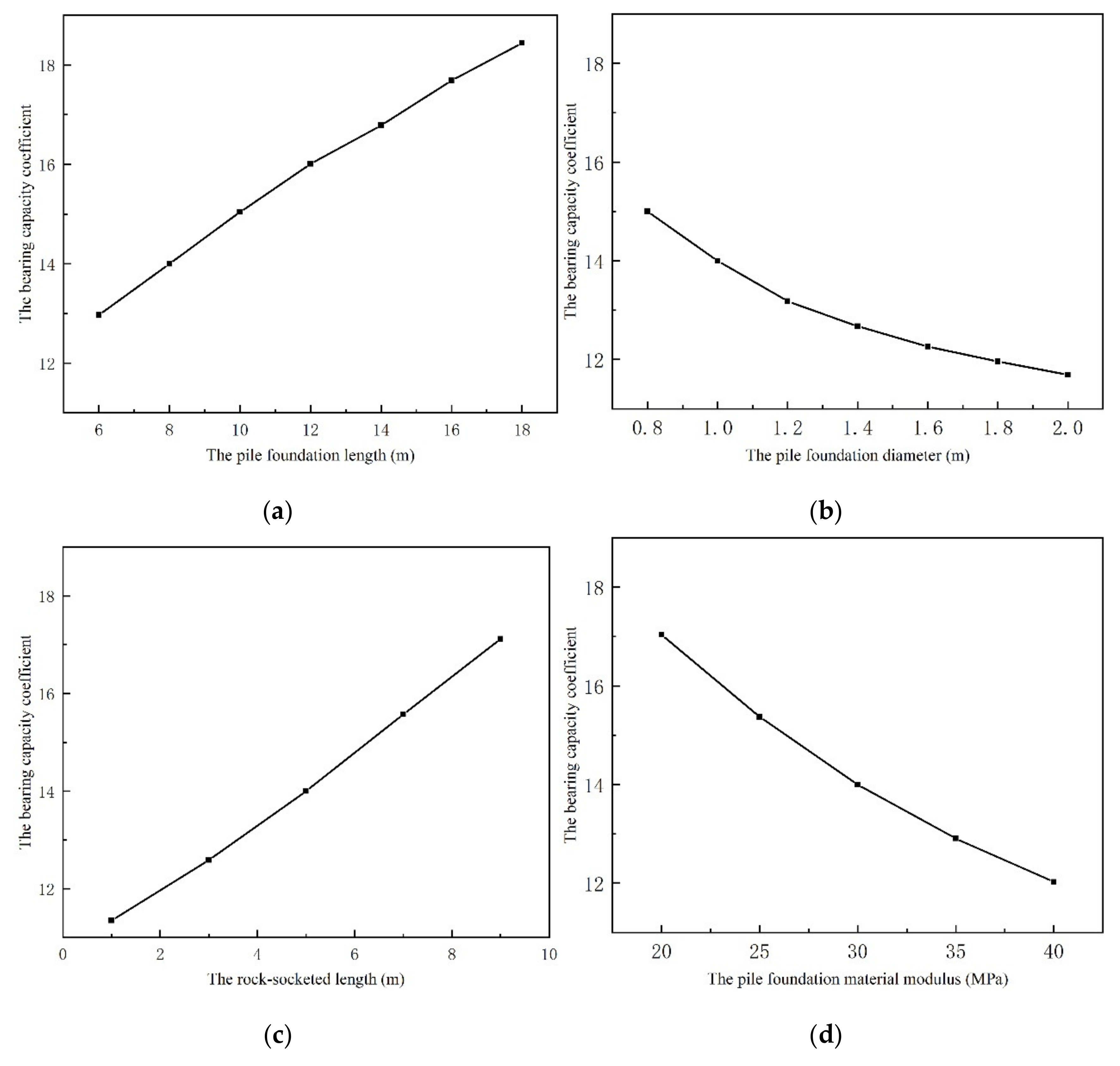
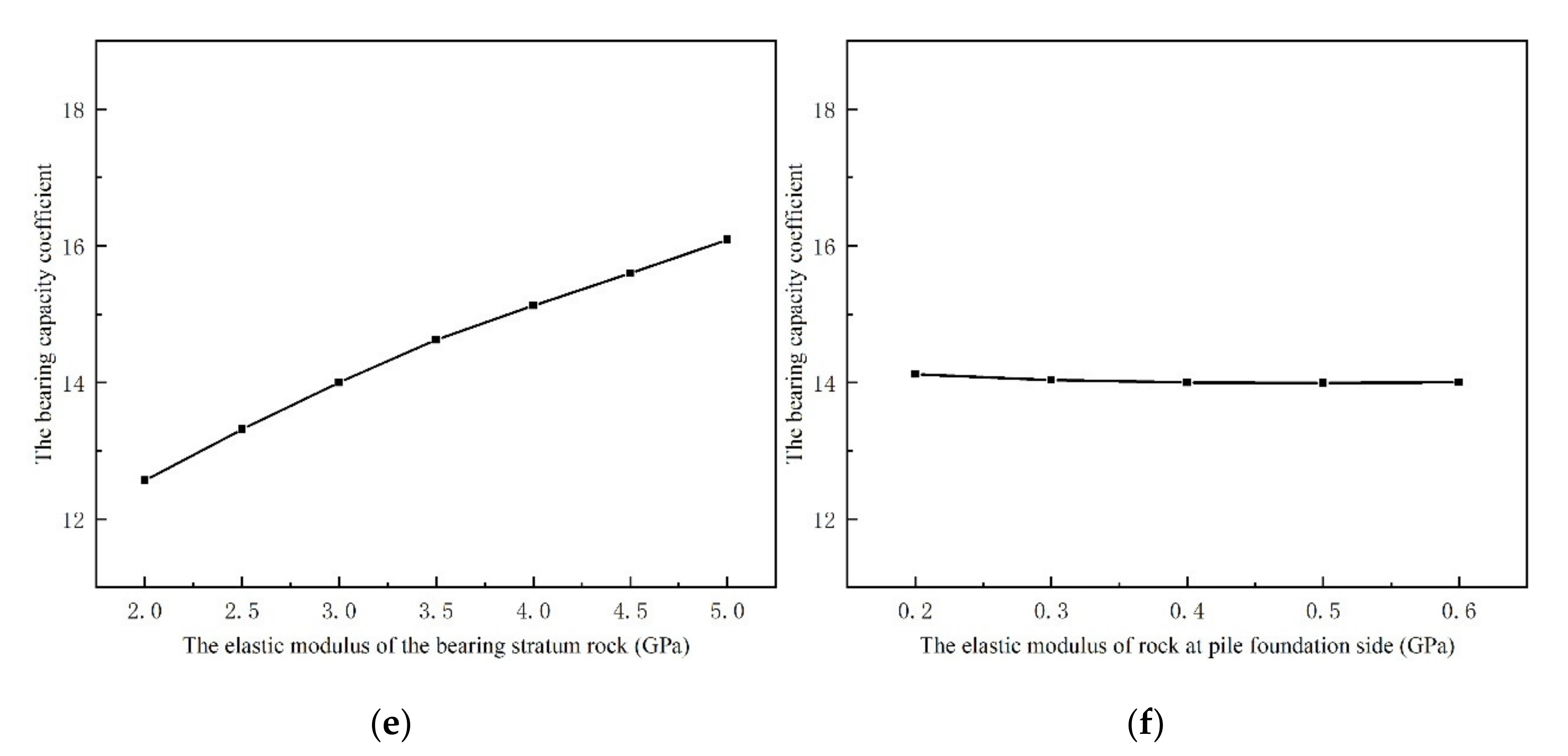
Many factors affect the bearing capacity and restraint stiffness of a single rock-socketed pile, including design parameters, engineering geology conditions, and construction factors. The geological situation is set, as the embedded rock is moderately weathered soft rock, and the overlying rock is strongly weathered soft rock. According to the properties of soft rock, the parameters are valued in ranges as follows: the elastic modulus of the bearing stratum rock is valued between 2.0 and 5.0 $GPa$, the elastic modulus of rock at the pile side is valued between 0.2 and 0.6 $GPa$, the pile body modulus is valued between 20.0 and 40.0 $GPa$, the pile length is valued between 6.0 and 18.0 m, the pile diameter is valued between 0.8 and 2.0 m, and the rock-socketed depth is valued between 1.0 to 9.0 $m$.

The ratio of the bearing capacity $R_a$ (calculated using Equation (24)) to the constraint stiffness $K_{vs}$ (calculated using Equation (25)), i.e., the bearing capacity coefficient λ, is proposed. With the parameters valued in the above ranges, the relationships between the parameters and the bearing capacity coefficient were calculated and are shown in Figure 3.

It can be seen from Figure 3 that the pile length, socketed depth, and pile modulus have a more significant impact on the bearing capacity coefficient, while the pile diameter and the bearing stratum rock modulus have a smaller influence. By comparison, the pile side rock modulus has no apparent impact on the bearing capacity coefficient, which is also the reason that rock-socketed piles are mostly end bearing piles.

2.5. Fitting of the Pile Bearing Capacity Coefficient

To obtain the bearing capacity coefficient λ, a multiple linear regression analysis was used, and the influence of a comprehensive coefficient $k$ with six control variables was considered. With the coefficient $\lambda$ as the dependent variable and the length of pile $L$, the diameter of pile $D$, the embedded rock elastic modulus $E_b$, the elastic modulus of surrounding rock $E_s$, the rock socketed depth $h$, and the pier elastic modulus $E_p$ as independent variables, the mathematical regression model of the bearing capacity coefficient is obtained:

$$\lambda =\frac{R_a}{K_{vs}}=k\left[c_{1}A{f}_{rk,b}+u{c}_{2}h{f}_{rk,b}+\frac{1}{2}{\varsigma }_{s}u\left(L-h\right)q_{sk}\right]\left(\frac{L}{EA}+\frac{1}{C_{0}A}\right)$$

(29)

$$k=a_0{L}^{a_1}{D}^{a_2}{E}_b^{a_3}{E}_s^{a_4}{h}_0{}^{a_5}{E}_p^{a_6}$$

(30)

where $a_0~a_6$ are the pending parameters, $f_{rk,b}$ is the saturated uniaxial compressive strength of the bearing stratum at the pile end, $q_{sk}$ is the lateral resistance of strongly weathered rock, and k is a comprehensive coefficient that can comprehensively reflect the influence of each variable on the bearing capacity and the constraint stiffness.

The numerical model with 120 sample data of the above six impact factors was established. With Formula (29) used as the calculation model, a multiple nonlinear regression was carried out. A loss function was used to minimize the sum of squared residuals, and the parameter was obtained by each iteration substituted into the loss function. When the sum of squared residuals is less than $1\times {10}^{-8}$ the iteration is terminated. After 190 iterations, the optimal solution is obtained, and the prediction regression model is:

$$\lambda =k\left[c_{1}A{f}_{rk,b}+u{c}_{2}h{f}_{rk,b}+\frac{1}{2}{\varsigma }_{s}u\left(L-h\right)q_{sk}\right]\left(\frac{L}{EA}+\frac{1}{C_{0}A}\right)$$

(31)

$$k=2866.669L^{-0.507}{D}^{0.237}{E}_b^{-0.704}{E}_s^{-0.009}{h}^{-0.267}{E}_p^{0.499}$$

(32)

The fitting results of all the sample data were evaluated with the coefficient of determination $R^2$. The closer the coefficient is to 1, the better the fitting effect is. After calculation, the fit degree was 0.997, which shows that the model can explain 99.7% of the variation, and the fitting degree is accurate.

3. Field Test and Numerical Simulation

3.1. Background Engineering

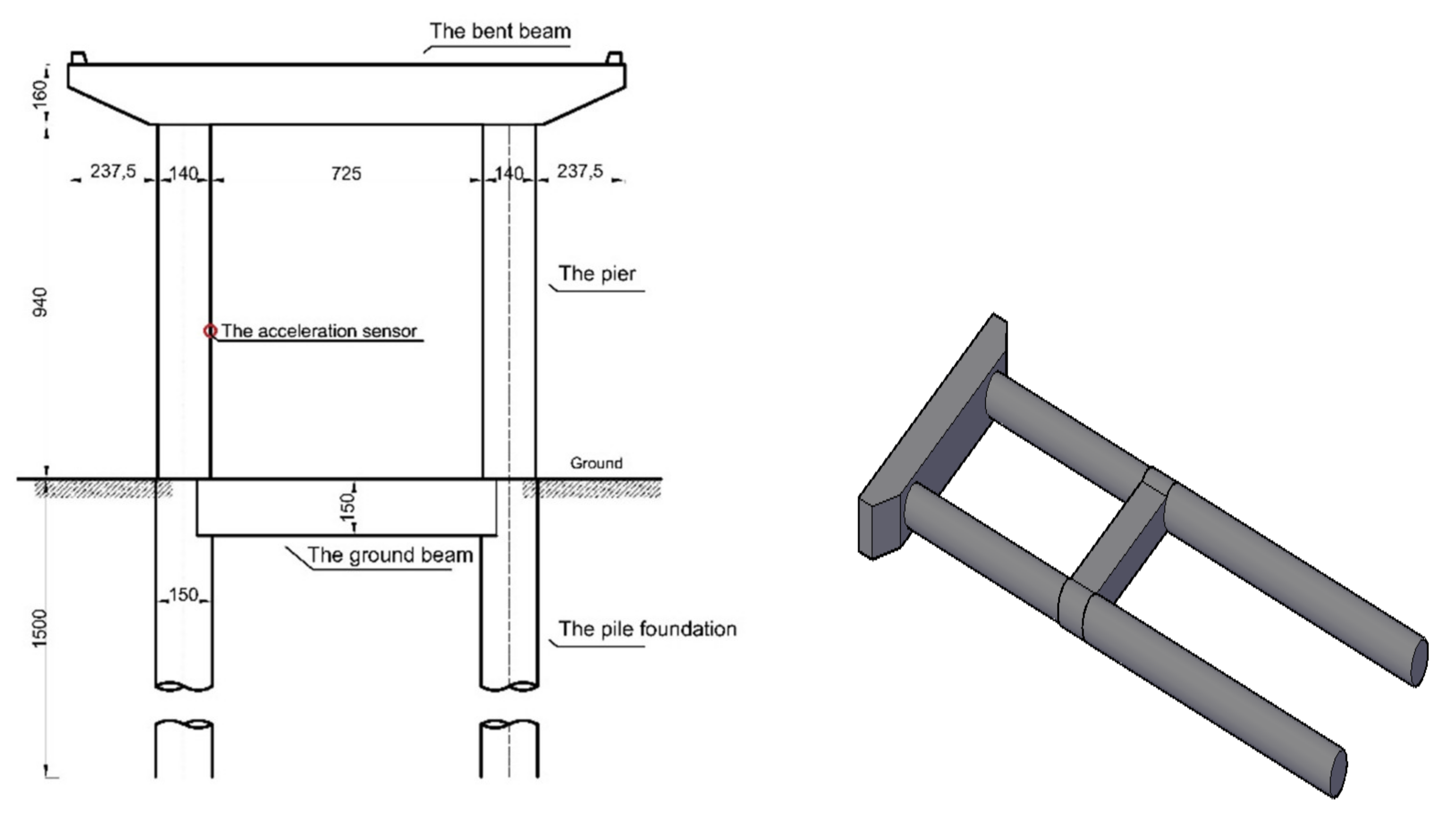
The background engineering is a uniform cross-section circular bridge pier of C40 concrete. The pier height is $9.4m$ and the diameter is$1.4m$. The pile foundation is a bored cast-in-place pile, the length of the pile is $15.0m,$ and the diameter is $1.5m$. The elevation of the test pier and pile is shown in Figure 4. The test pier is a double-pier column form, and the bent beam is consolidated with the piers at the pier top. The pier is consolidated with the pile foundation, and a ground beam connects the two pile foundations.

According to the design data, the mechanical properties of rock and soil layers at the bridge site are shown in

Table 1. Mechanical properties of rock and soil layers.

Type	Silty Clay	High-Weathered Argillaceous Siltstone	Medium-Weathered Argillaceous Siltstone
Compression modulus ($MPa$)	5.42	/	/
Cohesion force ($KPa$)	31.5	/	/
Friction angle ($°)$	18.1	/	/
Coefficient of friction on basis	0.25	0.4	0.45
Allowable bearing capacity ($KPa$)	160	320	1000
Standard value of soil friction resistance around the pile ($KPa$)	40	110	160
Uniaxial compressive strength of saturated rock ($MPa$)	/	/	11
Thickness ($m$)	1.1	5.34	8.56

.

3.2. Field Test Results of the Pier’s Fundamental Vertical Frequency

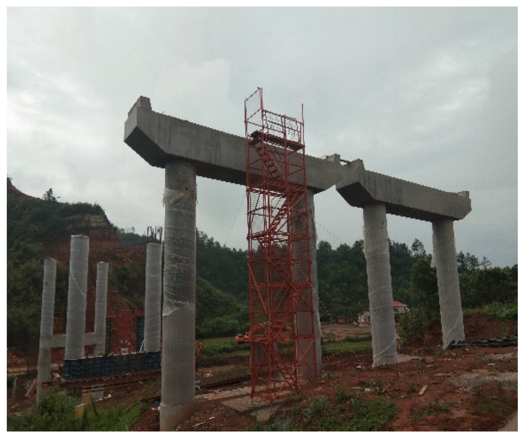
In the natural environment, structures vibrate slightly and irregularly with the surrounding vibration, and the structure’s slight vibration is pulsation. The pulsation has various frequencies, and the harmonic quantity of the structure’s fundamental frequency is the main component of the pulsation. The vertical fundamental frequency of the test pier was tested by the MGCplus dynamic data acquisition and analysis system. This system is accurate and reliable in dynamic tests and analyses. First, the dynamic signal was collected by the acceleration sensor and amplified by the amplifier. Then, the data was directly collected and recorded, and the acceleration time history curve was observed in real-time on the computer. Finally, with data post-processing software, the amplitude–frequency characteristics could be analyzed. The ultra-low frequency acceleration sensor was placed vertically on the pier side in the field test, as shown in Figure 4. The environmental vibration response of the pier was detected, and the MGCplus dynamic data acquisition and analysis system and computer at the other end read the detected signal. A photograph of the test pier pile is shown in Figure 5.

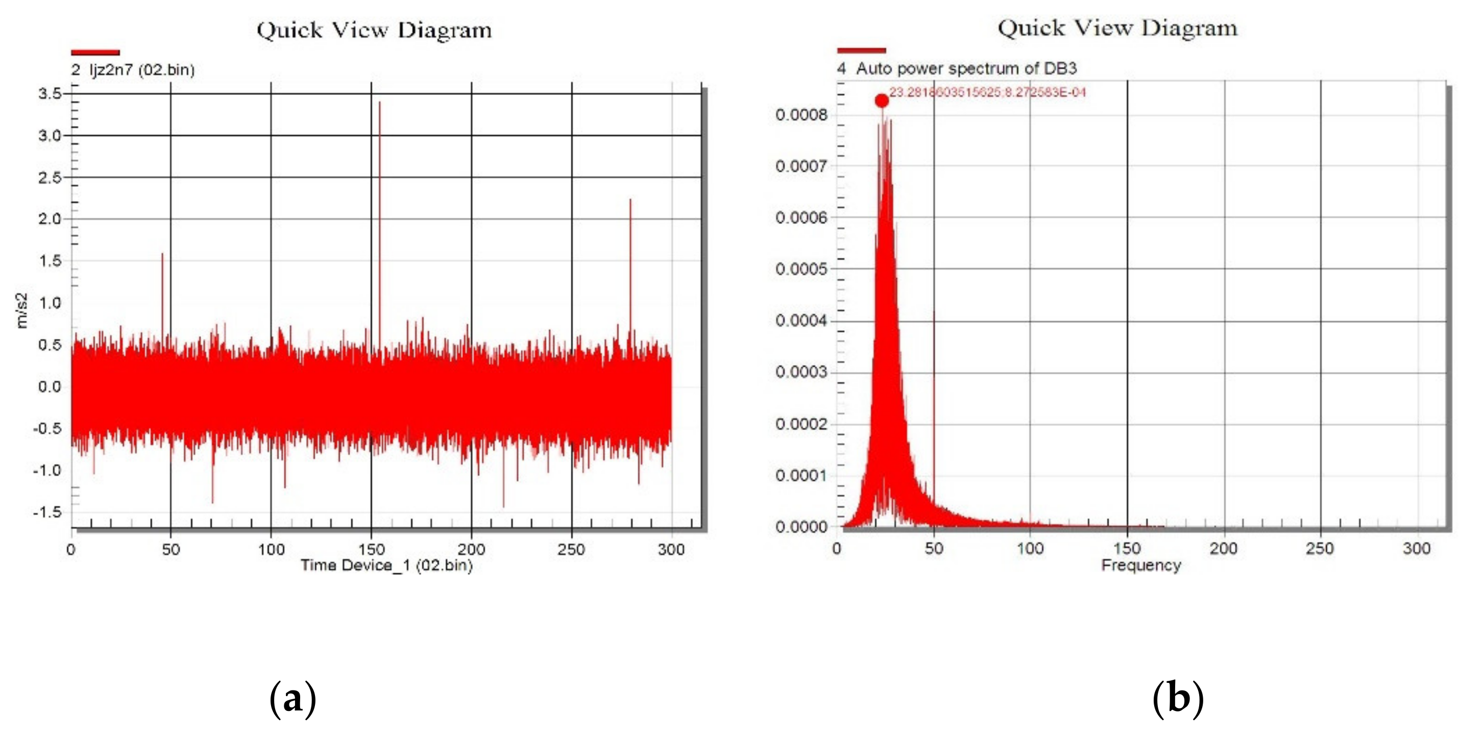
A group of three field tests on the dynamic characteristics of the pier was carried out using the pulsation method. One set of the results with the measured vertical acceleration time history curve and the frequency chart is shown in Figure 6.

Figure 6a shows the test bridge pier shaft to the acceleration time history diagram; using a filter to remove high- and low-frequency signal components and process the data by fast Fourier transformation, the frequency within the power spectral density curve was obtained, as shown in Figure 6b. The power spectrum peaks were determined by the frequency of each corresponding order of natural frequency. The first peak point was the fundamental frequency of the measured pier structure.

The pier’s measured vertical natural vibration frequencies were 23.282 Hz, 23.758 Hz, and 23.955 Hz. The three results are almost the same and indicate the method is accurate. Their average value is 23.665 Hz, and this was used as the vertical fundamental frequency.

3.3. Prediction of the Vertical Bearing Capacity

The pier fundamental frequency 23.665 Hz was used in Equation (23), and the other parameters of the test pier are shown in

Table 2. The test pier material’s design parameters.

Parameter	Value	Unit
Density $\rho$	2549	$\mathrm{kg}/{\mathrm{m}}^3$
Elastic modulus $E$	3.25 × 1010	$MPa$
Vertical fundamental frequency ${\omega }_{\nu }$	23.66	$Hz$
Mass of the pier top $M$	82,913.87	$kg$
Mass of the pier cap $m_c$	39,941.62	$kg$
Mass of the pier $m_d$	73,513.90	$kg$
Pier height $H$	9.4	$m$
Cross-section diameter $D$	1.5	$m$

based on the design data. The identified vertical constraint stiffness of the pile foundation $K_v$ was $2.715\times {10}^{9}N/m$ by Equation (23). The design vertical constraint stiffness $K_{vs}$ based on the code was calculated as $2.696\times {10}^{9}N/m$ by Equation (25).

The constraint stiffness identified by the frequency synthesis in this paper is about 0.7% larger than the calculated design value. The reasons are that the contribution of the pile side friction to the vertical stiffness was not considered in the code, and some parameters in the analytical formula were determined by interpolation. However, the difference between them is only about 0.7%, which indicates that it is accurate and feasible to identify the pier foundation vertical constraint stiffness by the frequency synthesis method.

Based on Equation (31), the bearing capacity coefficient $\lambda$ of the test pier is calculated as 15.62, and with the vertical constraint stiffness identified in the previous section, the pile’s bearing capacity is estimated at $42.41 MN$.

3.4. Finite Element Numerical Simulation

The actual structure was simplified to an axisymmetric finite element model for simulation. The finite element model of the test pile and rock-soil stratum was established by ABAQUS, and the CAX4R element (a 4-node bilinear axisymmetric quadrilateral, reduced integration, hourglass control) was used to simulate the pile and rock-soil stratum. In order to ensure the accuracy of the analysis and the efficiency of the calculation, the finite element mesh of the rock mass was divided into near pile and far pile. The model boundary conditions were set as follows. On the surface of the rock and the soil mass and cap, a free boundary was set. Then, after reaching a certain range of bedrock, the displacement of the pile top load was almost zero, so the surface was under the fixed displacement constraints. The lateral soil adopted horizontal displacement of the fixed constraints, and the vertical displacement of the free development of the pile side used the axial symmetry constraint. The pile bottom and rock mass were connected by Tie to achieve displacement coordination. The linear elastic constitutive model was used for the concrete pile, as the Mohr–Coulomb model is an ideal elastic-plastic model that can consider the influence of the stress state and stress history on the rock and soil and better simulate the nonlinear and dilatancy of the rock and soil. It was used for the rock-soil stratum. The contact pair algorithm was used to simulate the contact surfaces, as it can simulate the fracture, slip, and dislocation between the pile and soil-rock stratum. The normal behavior of the contact surfaces used the hard contact model. The pile and the rock-soil stratum can transfer normal pressure under the compression state, and the amplitude of the pressure is not limited. When there is a gap, the normal pressure is not transferred. The tangential behavior of contact surfaces used the friction model.

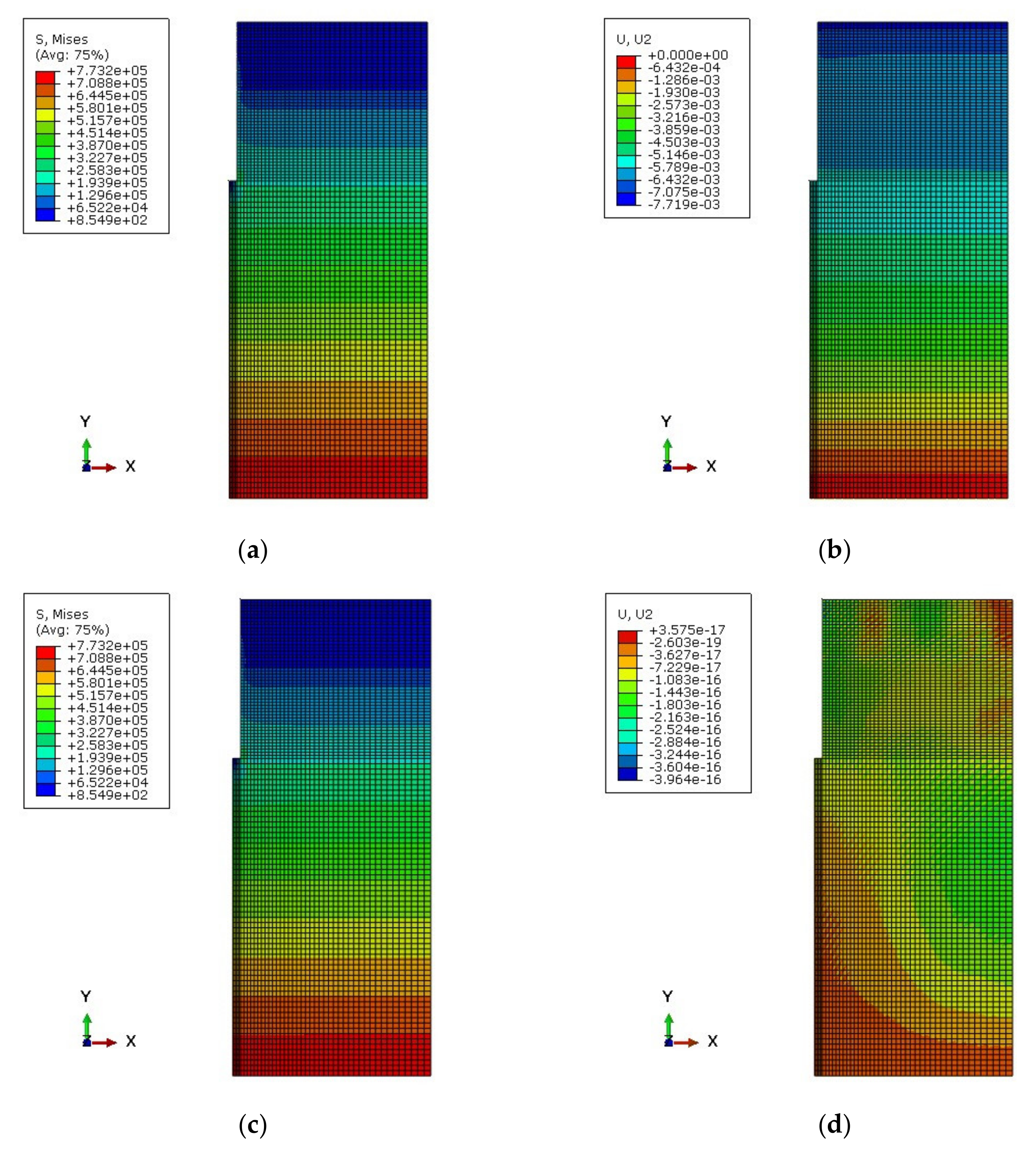
The initial equilibrium state of the pile rock-soil stratum system was established by the automatic ground stress balance step. Figure 7a,b show the distributions of stress and displacement before the initial stress equilibrium. Figure 7c,d show the distributions of stress and displacement after the initial stress equilibrium. Through comparison, it can be seen that the magnitude of stress remained unchanged after the stress equilibrium, and the magnitude of maximum displacement was 1 × 10⁻¹⁶ (m). Thus, the results of the initial ground stress equilibrium are precise enough for the finite element simulation.

4. Results and Discussion

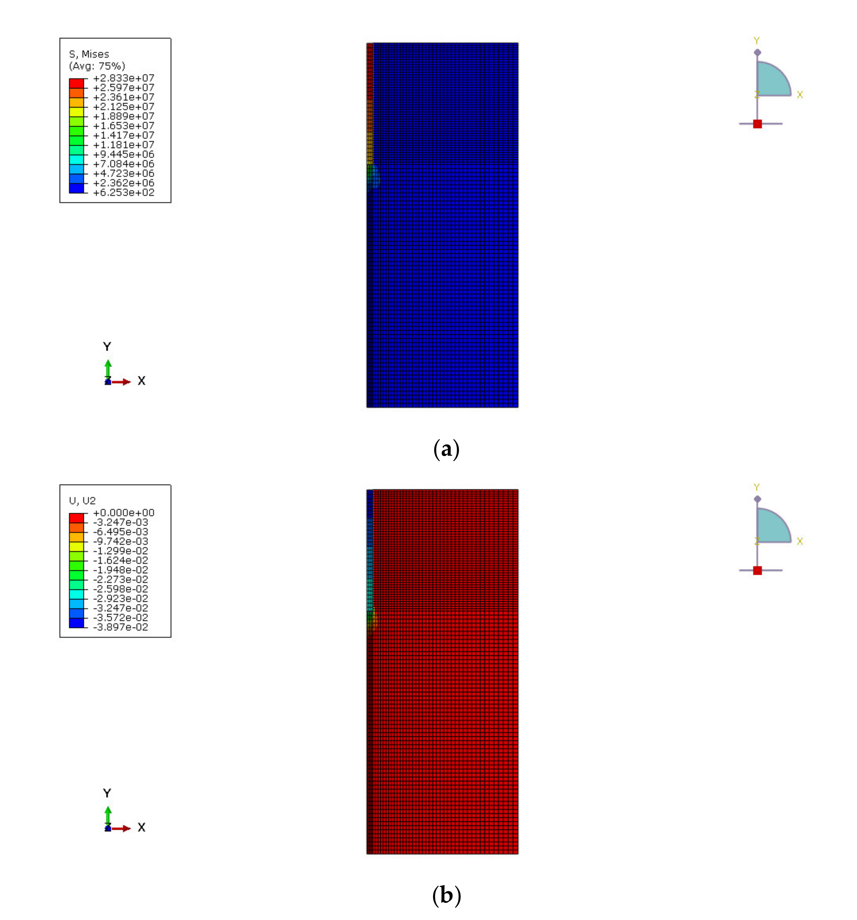
The stress distribution and deformation contour are shown in Figure 8.

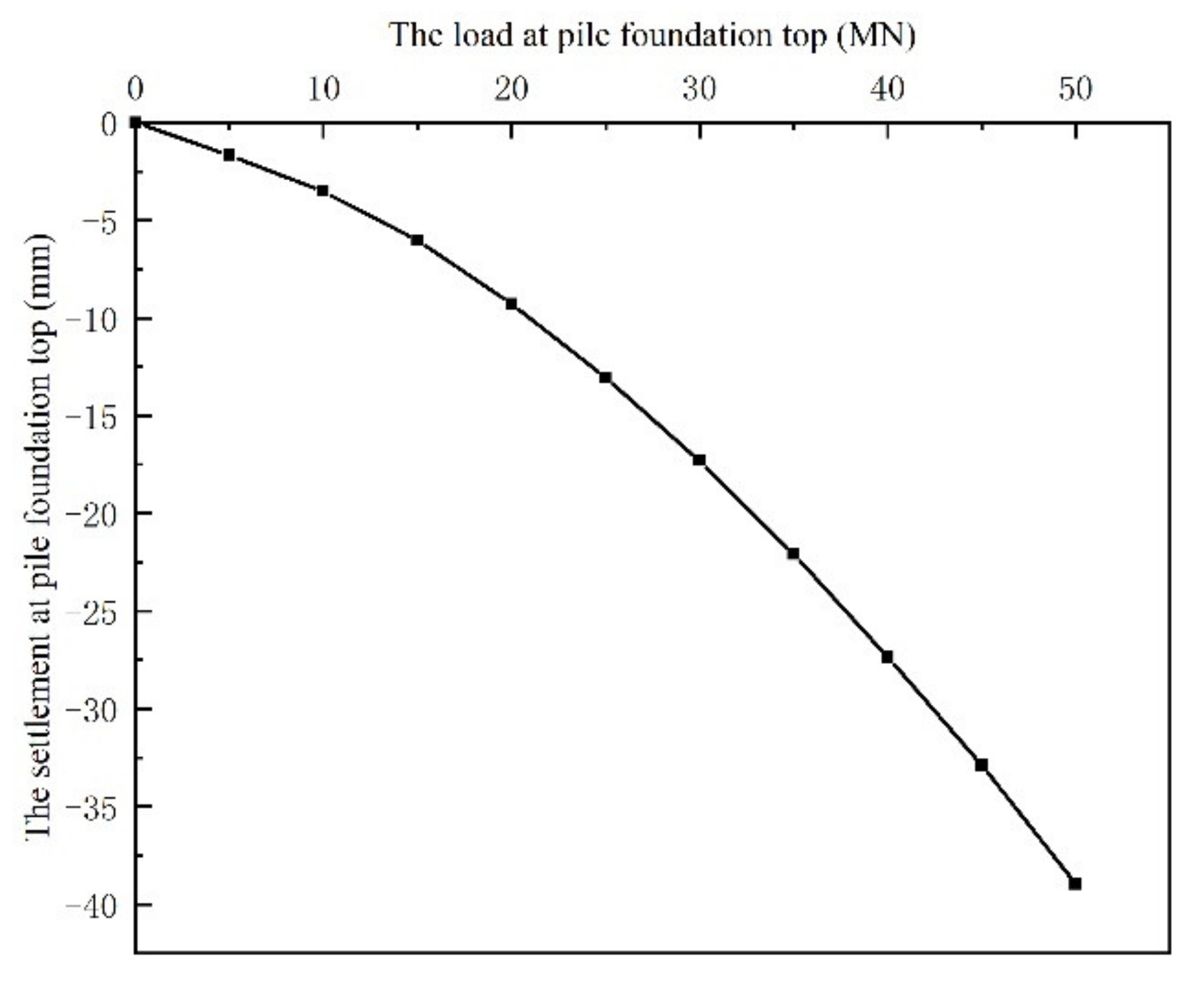
Figure 8a,b show the stress and the settlement of the pile top under a 50 MN load. The maximum stress in the pile was 28.33 MPa, and the maximum settlement at the pile top was 38.9 mm. The settlement of the pile top under different load levels was calculated, and the relationship between the settlement and the corresponding load is shown in Figure 9.

As the influence of settlement and the actual pile forming situation were not considered in the finite element simulation, the calculated bearing capacity was larger than the actual situation. Figure 9 shows that the load corresponding to the pile top settlement of $30 mm$ was $42.42\mathrm{MN}$. Compared with the bearing capacity (42.41 MN) calculated by the identification method in the previous section, the error was less than 1%. Furthermore, the reliability of the new method for predicting the bearing capacity of rock-socketed piles was proven.

5. Conclusions

In this paper, the analytical expression of the vertical restraint stiffness at the pier bottom was derived based on the Rayleigh energy method and the frequency synthesis method. The functional expression of the vertical restraint stiffness and the fundamental frequency of the pier was obtained. Then, the bearing capacity coefficients of the pile under different impact parameters were calculated and fitted by multiple nonlinear regression through the iterative algorithm. Based on the above results, a method to evaluate the bearing capacity of pile foundations is proposed. The main conclusions are as follows:

(1)

For the pier bearing capacity coefficient, the pile length, rock-socketed depth, and pile modulus have a more significant influence. The pile diameter and bearing stratum rock modulus have a smaller influence, whereas the side rock modulus has almost no impact. The bearing capacity coefficient increases with the increase of the pile length, socketed depth, and rock modulus, and it decreases with the increase of the pile diameter and pile modulus.

(2)

A new method for evaluating the vertical bearing capacity of a single pile is proposed. First, the analytical expression between the vertical fundamental frequency and the constraint stiffness of the pier is derived. Based on dynamic field tests, the pier frequency is measured. Then, through multiple regression, the bearing capacity coefficient model is obtained. Finally, with the design and measured data, the predicted bearing capacity of a single pile can be calculated.

(3)

According to the engineering example, the accuracy of the evaluation method was assessed through the finite element simulation calculation. The results showed that the error between the constraint stiffness calculated by the code and the constraint stiffness calculated by the frequency synthesis method was about 0.7%. The bearing capacity difference between the analytical solution and the finite element numerical simulation was small, and the method is accurate and effective.

References

- Zhou, C.Y.; Deng, Y.M.; Tan, X.S.; Liu, Z.Q.; Shang, W.; Zhan, S. Experimental research on the softening of mechanical properties of saturated soft rocks and application. Chin. J. Rock Mech. Eng. 2005, 24, 33–38. [Google Scholar]
- Wang, L.H.; Niu, C.Y.; Zhang, B.W.; Ma, Y.B.; Yin, S.J.; Xu, X.L. Experimental study on mechanical properties of deep-buried soft rock under different stress paths. Chin. J. Rock Mech. Eng. 2019, 38, 973–981. [Google Scholar]
- Coviello, A.; Lagioia, R.; Nova, R. On the measurement of the tensile strength of soft rocks. Rock Mech. Rock Eng. 2005, 38, 251–273. [Google Scholar] [CrossRef]
- Li, Q.; Tang, H. A Preliminary Framework of Standard Sequence Classification of Rock & Soil Strata. J. Eng. Geol. 2019, 27, 1188–1198. [Google Scholar]
- Khandelwal, M.; Armaghani, D.J. Prediction of drillability of rocks with strength properties using a hybrid GA-ANN technique. Geotech. Geol. Eng. 2016, 34, 605–620. [Google Scholar] [CrossRef]
- Kanji, M.A. Critical issues in soft rocks. J. Rock Mech. Geotech. Eng. 2014, 6, 186–195. [Google Scholar] [CrossRef] [Green Version]
- Gannon, J.A.; Masterton, G.G.T.; Wallace, W.A.; Wood, D.M. Piled Foundations in Weak Rock; Ciria: London, UK, 1999; p. 37. [Google Scholar]
- McVay, M.C.; Townsend, F.C.; Williams, R.C. Design of socketed drilled shafts in limestone. J. Geotech. Eng. 1992, 118, 1626–1637. [Google Scholar] [CrossRef]
- Zhang, Q.Q.; Ma, B.; Liu, S.W.; Feng, R.F. Behaviour analysis on the vertically loaded bored pile socketed into weak rocks using slip-line theory arc failure surface. Comput. Geotech. 2020, 128, 103852. [Google Scholar] [CrossRef]
- Singh, A.P.; Bhandari, T.; Ayothiraman, R.; Rao, K.S. Numerical analysis of rock-socketed piles under combined vertical-lateral loading. Procedia Eng. 2017, 191, 776–784. [Google Scholar] [CrossRef]
- Hassan, K.M.; O’Neill, M.W.; Sheikh, S.A.; Ealy, C.D. Design method for drilled shafts in soft argillaceous rock. J. Geotech. Geoenviron. Eng. 1997, 123, 272–280. [Google Scholar] [CrossRef]
- Zhao, M.; Zou, X.; Liu, Q. Loading Test on the Vertical Bearing Capacty of Super-Long and Large-Diameter Bored Piles in the Soft Soil Area of Dongting Lake. China Civ. Eng. J. 2004, 10, 63–67. [Google Scholar]
- Zhao, M.; Xia, R.; Yin, P.; Yang, C.; Xu, Z. Load transfer mechanism of socketed piles considering shear dilation effects of soft rock. Chin. J. Geotech. Eng. 2017, 36, 1005–1011. [Google Scholar]
- Ter-Martirosyan, Z.; Ter-Martirosyan, A.; Sidorov, V. Settlement and Bearing Capacity of the Pile in A Three-Layer Base Taking into Account the Elastic-Visco-Plastic Properties of Soils. In IOP Conference Series: Materials Science and Engineering; IOP Publishing: Bristol, UK, 2019; Volume 661, p. 012099. [Google Scholar]
- Cai, Y.; Xu, B.; Cao, Z.; Geng, X.; Yuan, Z. Solution of the ultimate bearing capacity at the tip of a pile in inclined rocks based on the Hoek-Brown criterion. Int. J. Rock Mech. Min. Sci. 2020, 125, 104140. [Google Scholar] [CrossRef]
- Williams, A.F.; Johnston, I.W.; Donald, I.B. The design of socketed piles in weak rock. In Proceedings of the International Conference on Structural Foundations on Rock, Sydney, Australia, 7–9 May 1980; Volume 1, pp. 327–347. [Google Scholar]
- Józefiak, K.; Zbiciak, A.; Maślakowski, M.; Piotrowski, T. Numerical modelling and bearing capacity analysis of pile foundation. Procedia Eng. 2015, 111, 356–363. [Google Scholar] [CrossRef]
- Zhan, C.; Yin, J.H. Field static load tests on drilled shaft founded on or socketed into rock. Can. Geotech. J. 2000, 37, 1283–1294. [Google Scholar] [CrossRef]
- Huang, B.; Zhang, Y.; Lv, B.; Yang, Z.; Fu, X.; Zhang, B. Vertical bearing characteristics of rock-socketed pile in a synthetic soft rock. Eur. J. Environ. Civ. Eng. 2021, 25, 132–151. [Google Scholar] [CrossRef]
- Nallim, L.G.; Grossi, R.O. A general algorithm for the study of the dynamical behaviour of beams. Appl. Acoust. 1999, 57, 345–356. [Google Scholar] [CrossRef]
- Wang, J.; Wang, F. Approximate algorithm of compound fundamental frequencies of tapered bridge piers. J. Southeast Univ. 2005, 4, 580–583. [Google Scholar]
- Grossi, R.O.; Albarracín, C.M. Some observations on the application of the Rayleigh–Ritz method. Appl. Acoust. 2001, 62, 1171–1182. [Google Scholar] [CrossRef]
- Chen, J.; Li, D. Frequency composition method of tapered pier of tall-piered continuous beam bridge. J. Railw. Sci. Eng. 2008, 3, 28–31. [Google Scholar]
- Lipeng, A.; Dejian, L. An analytical algorithm based on frequency synthesis method for calculating transverse vibration frequency of single column pier with pile foundation. Chin. J. Appl. Mech. 2015, 32, 524–529. [Google Scholar]
- Feng, Z.J.; Chen, H.Y.; Yuan, F.B. Vertical bearing characteristics of bridge pile foundation under pile-soil-fault coupling. J. Transp. Eng. 2019, 19, 36–48. [Google Scholar]
- Gao, G.; Gao, M.; Chen, Q.; Yang, J. Field load testing study of vertical bearing behavior of a large diameter belled cast-in-place pile. KSCE J. Civ. Eng. 2019, 23, 2009–2016. [Google Scholar] [CrossRef]
- Peng, B.X.; Wang, X.H. Research on bearing capacity of Cretaceous argillaceous siltstone. Yanshilixue Yu Gongcheng Xuebao/Chin. J. Rock Mech. Eng. 2005, 24, 2678–2682. [Google Scholar]
- Horvath, R.G.; Kenney, T.C.; Kozicki, P. Methods of improving the performance of drilled piers in weak rock. Can. Geotech. J. 1983, 20, 758–772. [Google Scholar] [CrossRef]
Figure 1.
The vertical translation and deformation of the pier.
Figure 2.
Combinations of vertical displacement elements and mass elements.
Figure 3.
The bearing capacity coefficient curves with different parameters: (a) the pile foundation length, (b) the pile foundation diameter, (c) the rock-socketed length, (d) the pile foundation modulus, (e) the modulus of the bearing stratum rock, and (d) the modulus of rock at pile foundation.
Figure 4.
The elevation of the test pier. (Units: )
Figure 5.
Field photograph of the test pier.
Figure 6.
(a) The vertical acceleration time history curve; (b) the measured pier vertical fundamental frequency.
Figure 7.
(a) The stress distribution before the ground stress equilibrium; (b) the displacement distribution before the ground stress equilibrium; (c) the stress distribution after the ground stress equilibrium; (d) the displacement distribution after the ground stress equilibrium.
Figure 8.
(a) The equivalent stress distribution of the pile-rock stratum model; (b) the deformation of the pile-rock stratum model.
Figure 9.
The relationship between the settlement and the load at the pile foundation.