Comment on the Determination of the Polar Anchoring Energy by Capacitance Measurements in Nematic Liquid Crystals

Abstract

Capacitance measurements have been extensively used to measure the anchoring extrapolation length L at a nematic–substrate interface. These measurements are extremely delicate because the value found for L often critically depends on the sample thickness and the voltage range chosen to perform the measurements. Several reasons have been proposed to explain this observation, such as the presence of inhomogeneities in the director distribution on the bounding plates or the variation with the electric field of the dielectric constants. In this paper, I propose a new method to measure L that takes into account this second effect. This method is more general than the one proposed in Murauski et al. Phys. Rev. E 71, 061707 (2005) because it does not assume that the anchoring angle is small and that the anchoring energy is of the Rapini–Papoular form. This method is applied to a cell of 8CB that is treated for planar unidirectional anchoring by photoalignment with the azobenzene dye Brilliant Yellow. The role of flexoelectric effects and the shape of the anchoring potential are discussed.

1. Introduction

Measuring the anchoring energy W of the director at the bounding plates of a nematic cell is necessary to predict its electrooptical properties under electric field. This is important from a basic physics perspective to better understand anchoring phenomena [1,2,3] and for applications in electro-optic devices, such as LCD displays, to improve their performance [4]. More specifically in this paper, I focus on the measurement of the polar anchoring energy in planar cells filled with a liquid crystal (LC) of positive dielectric anisotropy. This measurement is very classical, but nonetheless extremely delicate as one immediately realizes after reading the literature on this subject. Indeed, the value of W obtained with the same LC and the same substrates may differ by several orders of magnitude when measured by different groups [5]. In practice, various techniques have been proposed to measure the anchoring extrapolation length $L=K_1/W$, from which W can be deduced knowing the splay elastic constant $K_1$. Some of the techniques analyze the deformation of the director field in the presence of a wall [6] or in a wedge cell [7,8,9]. Others use light scattering [10,11,12]. However, the most widely used techniques are based on the action of an external field. Among them, one can cite all-optical methods using magnetic or electric field as the ones described by Subacius et al. [13] or Murauski et al. [14] and much more standard methods using an electric field and capacitance and/or optical retardation measurements. In this last category, the method proposed by Yokoyama and van Sprang [15] at high electric field (YvS method) is certainly the most popular. This method consists of plotting $R/R_0$ as a function of $1/CV$. Here, V is the applied voltage, C is the capacitance, and R is the optical retardation between the ordinary and extraordinary rays (with the index 0 denoting that the measurement has been performed without electric field). The model predicts that in a certain range of voltage, $V_{\min }<V<V_{\max }$, the curve must be a line whose intersection with the ordinate axis gives W. The first inequality with $V_{\min }\approx 6V_c$, where $V_c$ is the Fréedericksz voltage, ensures that the tilt angle ${\varphi }_m$ in the middle of the cell is equal to $\pi /2$ to better than ${10}^{-3}$rad. The second inequality ensures that the tilt angle on the plates, $\theta$, remains small enough sor that the actual anchoring potential is approximately given by the Rapini–Papoular formula $W\left(\theta \right)=\frac{1}{2}W{sin}^2\theta$ [16]. By assuming that this is the case for $\theta <0.2$rad, the calculation shows that $V_{\max }\approx \frac{0.2}{\pi }\sqrt{\frac{{\epsilon }_{\perp }}{{\epsilon }_{\Vert }}}\frac{d}{L}{V}_c$ [17]. In practice, Nastishin et al. have shown that similar results can be obtained by just measuring the optical retardation in the same range of voltage (RV method) [5,17]. This method is interesting because it allows a local measurement of L. The problem with these two methods is that they often give very different values of L depending on the voltage interval $(V_1,V_2)$ chosen to perform the fit of the experimental data, even when $(V_1,V_2)\in (V_{\min },V_{\max })$. Even the unphysical negative value of $W_a$ can be obtained [17]. According to Nastishin et al. [17], this unexpected behavior could be due to in-plane inhomogeneities of the cell (variations of the anchoring energy, easy axis, fractures in the patterned electrodes, etc.), thus making these methods difficult to use to determine a reliable value for W.

In this paper, I propose an alternative method to measure the polar (zenithal) anchoring energy W in a planar cell based on capacitance measurements at high electric field. The main difference with previous works is that I take into account the variation of the dielectric constant ${\epsilon }_{\Vert }$ with the electric field and I use the full integral equations to fit the experimental data. This way, the limitation to small tilt angles on the plates is waived and any form of the anchoring potential can be used. I will show that these improvements are necessary to obtain consistent results when the measurements are performed in thin samples under high electric field. The experiments will be performed using the LC 8CB (4-octyl-4’-cyanobiphenyl) and the electrodes are treated for planar unidirectional anchoring by photoalignment with the azo-dye Brilliant Yellow (BY) [18,19,20]. With this treatment, there is no pretilt angle at the electrodes, which simplifies the problem.

2. Basic Equations

Let us consider a planar sample. The x-axis is taken parallel to the anchoring direction on the electrodes and the z-axis is perpendicular to the electrodes, with $z=0$ at the bottom electrode and $z=d$ at the top electrode. I denote by $\varphi \left(z\right)$ the tilt angle of the director with respect to the x-axis and by $\theta$ the tilt angle on the electrodes ($\theta =\varphi \left(0\right)=\varphi \left(d\right)$). I suppose that there is no pretilt angle, which means that $\theta =0$ when no electric field is applied. For now, the anchoring potential is assumed to be of the Rapini–Papoular form [16]

$$W\left(\theta \right)=\frac{1}{2}W{sin}^2\theta ,$$

(1)

and I neglect the flexoelectric effect. When an electric field is applied and the anchoring is very strong the sample destabilizes above the Fréedericksz critical voltage $V_c$, given by [1,21]

$$V_c=\pi \sqrt{\frac{K_1}{{\epsilon }_0{\epsilon }_a}}.$$

(2)

In this equation, ${\epsilon }_0$ is the vacuum permittivity, ${\epsilon }_a={\epsilon }_{\Vert }-{\epsilon }_{\perp }$ is the dielectric anisotropy of the nematic phase and $K_1$ is the splay constant. The actual critical voltage $V_c^{\prime }$ is slightly smaller if the anchoring energy is taken into account and it is the solution of the following equation [1,16]:

$$\frac{d}{L}=\pi \frac{V_c^{\prime }}{V_c}tan\left(\frac{\pi V_c^{\prime }}{2V_c}\right),$$

(3)

where $L=K_1/W$ is the anchoring extrapolation length. This equation shows that the ratio $d/L$ must be larger than $\approx 200$ for $V_c^{\prime }\approx V_c$ to better than 1%.

The formulas that give the capacitance as a function of the applied voltage are well known [22,23] and are recalled in [24]. They considerably simplify at large voltage, when the maximum tilt angle ${\varphi }_m$ in the middle of the cell is very close to $\pi /2$. Numerical calculations show that this condition is typically satisfied when $V\gtrsim 6V_c$. In this limit, ${\varphi }_m\approx \pi /2$ to better than ${10}^{-3}$rad [5]. If the flexoelectric effects are screened out by the ions contained in the LC–and this is usually the case experimentally–the capacitance can be calculated by using the formula [25]:

$$\frac{C}{C_{\perp }}=1+\gamma -\frac{2}{\pi }\gamma \sqrt{1+\gamma }\frac{V_c}{V}{\int }_{sin\theta }^1\sqrt{\frac{1+\kappa x^2}{1+\gamma x^2}}\mathrm{d}x,$$

(4)

where $\gamma ={\epsilon }_{\Vert }/{\epsilon }_{\perp }-1$ and $\kappa =K_3/K_1-1$ (with $K_3$ the bend constant) and $C_{\perp }={\epsilon }_0{\epsilon }_{\perp }S/d$ is the capacitance measured below the onset of instability (with S the surface area of the electrodes).

The surface angle $\theta$ is obtained by solving the surface torque equation which reads by using the Rapini–Papoular potential [26]:

$$sin\theta =\sqrt{\frac{1+\kappa {sin}^2\theta }{1+\gamma {sin}^2\theta }}\frac{\pi }{\sqrt{1+\gamma }}\frac{L}{d}\frac{V}{V_c}\frac{C}{C_{\perp }}.$$

(5)

Solving these two equations can determine the ratio $C/C_{\perp }$ as a function of $V/V_c$ provided that $\kappa$, $\gamma$ and the ratio $L/d$ are known.

If $\theta$ is small, expanding the two previous equations in power series of $sin\theta$ yields [27]

$$\frac{C}{C_{\perp }}=\frac{1+\gamma }{1-2\gamma \frac{L}{d}}-\frac{2}{\pi }\frac{\gamma \sqrt{1+\gamma }}{1-2\gamma \frac{L}{d}}I\frac{V_c}{V},$$

(6)

where $I\equiv {\int }_0^1\sqrt{\frac{1+\kappa x^2}{1+\gamma x^2}}\mathrm{d}x$. This equation is valid as long as $\frac{2}{3}(\kappa -\gamma ){sin}^3\theta \ll I$, i.e., as long as ${sin}^3\theta \ll 1$ since I and $\kappa -\gamma$ are usually measured to be of order unity. This imposes that the voltage is not too large, typically less than voltage $V_{\max }$ defined in the introduction for $\theta <0.2$rad. Note that these equations can also be applied to homeotropic samples by exchanging ${\epsilon }_{\Vert }$ and ${\epsilon }_{\perp }$ and $K_1$ and $K_3$, and by redefining $\theta$ as the angle between the director and the normal to the plates [28].

To summarize, the theory predicts that the reduced capacitance $\overline{C}=C/C_{\perp }$ must vary linearly as a function of the inverse of the reduced voltage $\overline{V}=V/V_c$ provided that $V_1<V<V_2$ as in the YvS or RV models.

This calculation thus predicts that fitting with a line the capacitance curve $\overline{C}(1/\overline{V})$ in any voltage range $(V_1,V_2)$ satisfying $V_1>V_{\min }$ and $V_2<V_{\max }$ should allow to determine L and the elastic anisotropy $\kappa$ provided that d, $C_{\perp }$, $V_c$ and the dielectric anisotropy $\gamma$ are known precisely. Indeed, the value at the origin of the regression line gives $L/d$ while its slope gives I, and thus $\kappa$, provided $\gamma$ is known.

In the following, I show that this method, as the YvS method or the RV method, fails to yield correct measurements of L and I explain why. I then show how to improve the fitting procedure to obtain a reliable value for L.

3. Experimental Results

3.1. Sample Preparation and Experimental Setup

The LC chosen is 8CB. It was purchased from Synthon (Germany) and used without further purification. I measured the nematic-to-smectic A transition temperature $T_{\mathrm{NA}}=33.8{}^{\circ }$C and the nematic-to-isotropic transition temperature $T_{\mathrm{NI}}=40.75{}^{\circ }$C. All the samples were prepared between two ITO (Indium Tin Oxide)-coated glass plates. A thin band of ITO was removed on the sides of the plates and the metallic wires used to measure the capacitance were soldered on the ITO surface with an ultrasonic soldering system in order to decrease the parasitic capacitances. Nickel wires were used as a spacer to fix the sample thickness and a slow-cure epoxy glue was used to bond them together. To reduce the uncertainties, thin samples ($d\approx 7.5\mathsf{\mu }$m) with large surface area ($S\approx 2.5$ cm${}^2$) were used to measure the dielectric constants, while a thick sample ($d\approx 50\mathsf{\mu }$m) was used to measure $V_c$. In all samples, a special care was taken to ensure the parallelism between the two glass plates, always better than $5\times {10}^{-5}$rad. The thickness of the empty cells was measured with an Ocean Optics USB2000 spectrometer. The dielectric constant ${\epsilon }_{\perp }$ was measured using homeotropic samples. In that case, the glass plates were treated with the polyimide Nissan SE-4811. The polyimide was deposited by spin-coating and the plates were then baked at 180 ${}^{\circ }$C for 30 min. The measurements of ${\epsilon }_{\Vert }$ and L were performed using planar samples. The unidirectional planar anchoring was achieved by photoalignment using a commercial azo-dye, Brilliant Yellow, sold by Sigma. The dye was dissolved in DMS (0.3% by weight) and then deposited by spin-coating at 2000 rpm during 30 s. Before that, the plates were cleaned with sulfochromic acid, flushed with distilled water and dried at 100 ${}^{\circ }$C during 15 min. Once the dye was deposited, the plates were baked at 95 ${}^{\circ }$C for 30 min. The unidirectional planar anchoring was obtained by illuminating the plates during 30 min under normal incidence with the linearly polarized parallel light beam of a mercury vapor lamp equipped with a filter at $\lambda =436$nm. The power of the light beam was 1.1 mW/cm${}^2$, so the exposure dose was close to 2 J/cm${}^2$. The relative humidity in the room, which is another important parameter according to Wang et al. [29], was close to 40% during all the steps of preparation of the sample. With this protocole a strong planar anchoring was obtained, with no pretilt angle. All the capacitance measurements were performed at 5 kHz in the dielectric regime of the LC (I measured a charge relaxation frequency close to 500 Hz in 8CB) with a HP 4284A LCR meter, initially calibrated with standard capacitors. All the cells were filled by capillarity in the isotropic phase. Finally, the samples were placed into a home-made oven regulated to within $\pm 2$mK thanks to an ATNE ATSR 100 PID controller.

3.2. Measurement of the Dielectric Constants ${\epsilon }_{\Vert }$ and ${\epsilon }_{\perp }$

I first measured the two dielectric constants. In usual experiments, ${\epsilon }_{\perp }$ is obtained by measuring the capacitance $C_{\perp }$ of a planar sample below the onset of Fréedericksz instability and ${\epsilon }_{\Vert }$ is deduced from an extrapolation to 0 of the capacitance curve $C(1/V)$ by assuming that $L/d\ll 1$. This requires the use of very thick samples (except if the anchoring is very strong, which we do not know a priori) and, in that case, the capacitance measurements are less precise.

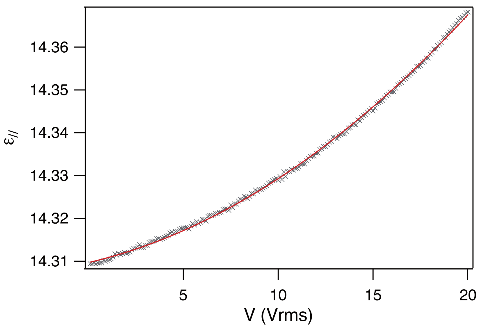
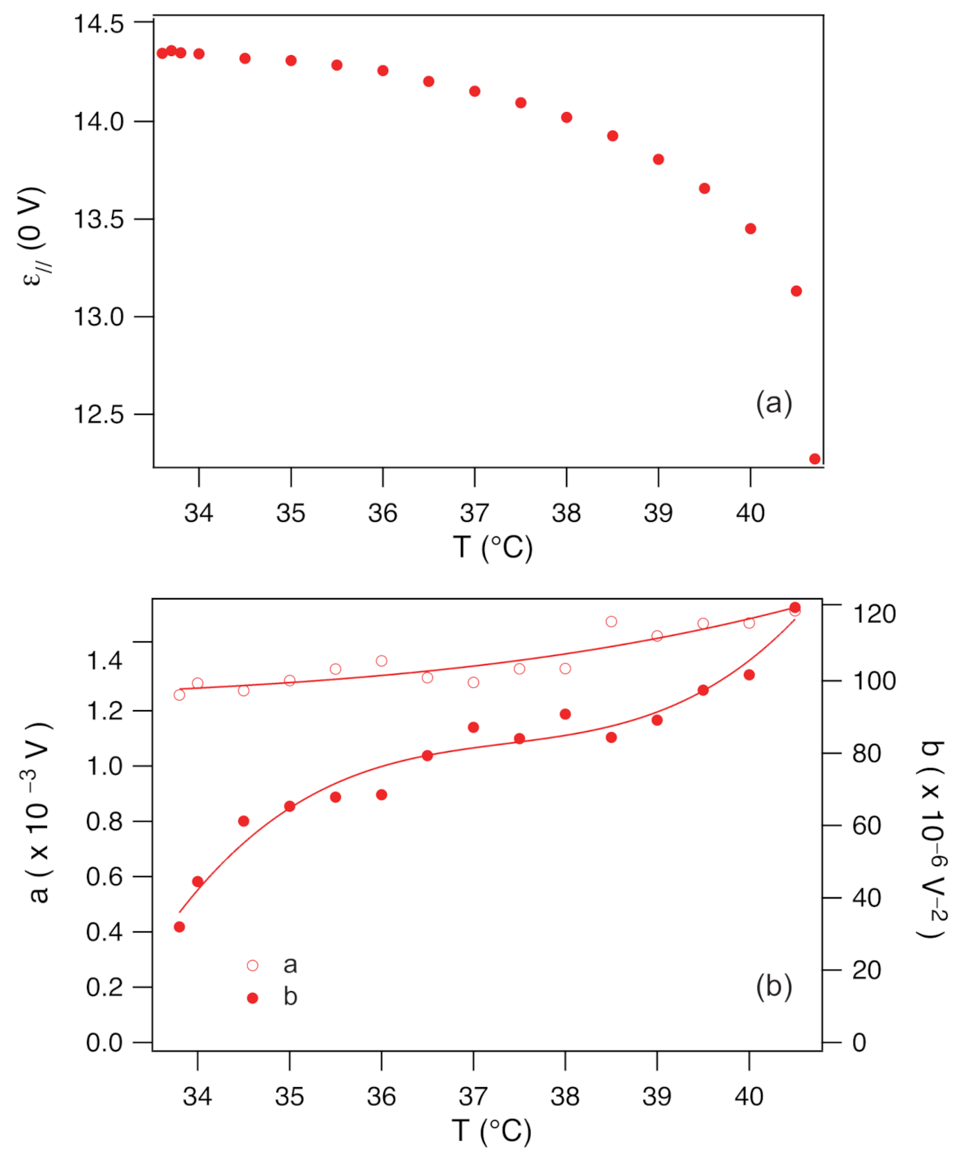
To avoid this difficulty, I directly measured ${\epsilon }_{\Vert }$ using a thin homeotropic sample of thickness $d=7.5\mathsf{\mu }$m. Measurements were performed between 0.1 and 20 Vrms by step of 0.1 Vrms and 2 s per step. The dielectric constant ${\epsilon }_{\perp }$ was obtained by dividing the measured capacitance by the capacitance of the empty cell measured at the same voltage. In this way, I noticed that ${\epsilon }_{\Vert }$ was not strictly constant, but increased slightly when the electric field was increased (Figure 1). This phenomenon is well known and is due to two effects. The first one is due to a freezing of the director fluctuation modes that leads to a linear increase in ${\epsilon }_{\Vert }$ with the electric field [30]. The second is the Kerr effect which is microscopic in origin. It leads to a quadratic increase in the quadrupolar parameter order [31], and thus of ${\epsilon }_{\Vert }$, as a function of the electric field. This behavior is well verified in my experiments, as shown in Figure 1. In this example, the experimental data are well fitted by a law of the form ${\epsilon }_{\Vert }={\epsilon }_{\Vert }\left(0\right)+aE+b{E}^2$ [32]. The same behavior is observed at all temperatures. The temperature dependence of ${\epsilon }_{\Vert }\left(0\right)$ and of the fit coefficients a and b is shown in Figure 2.

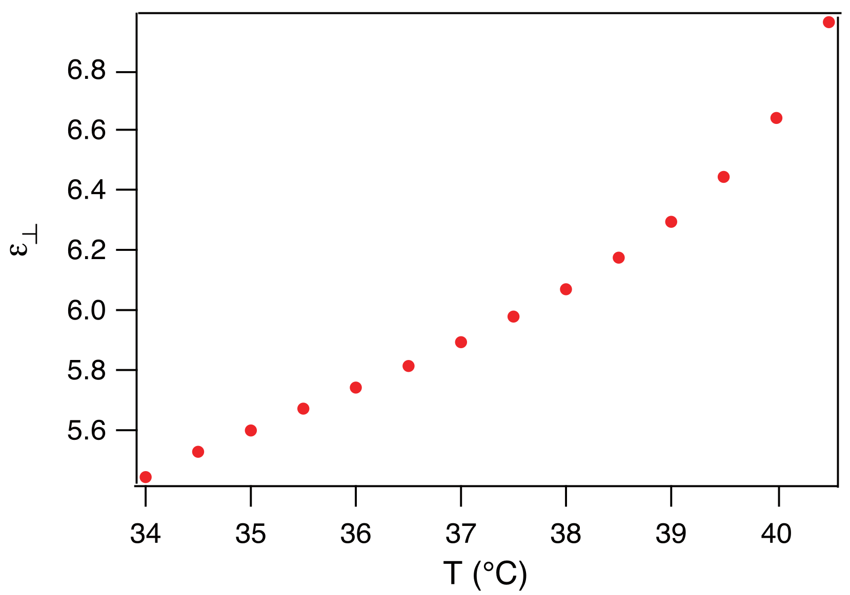
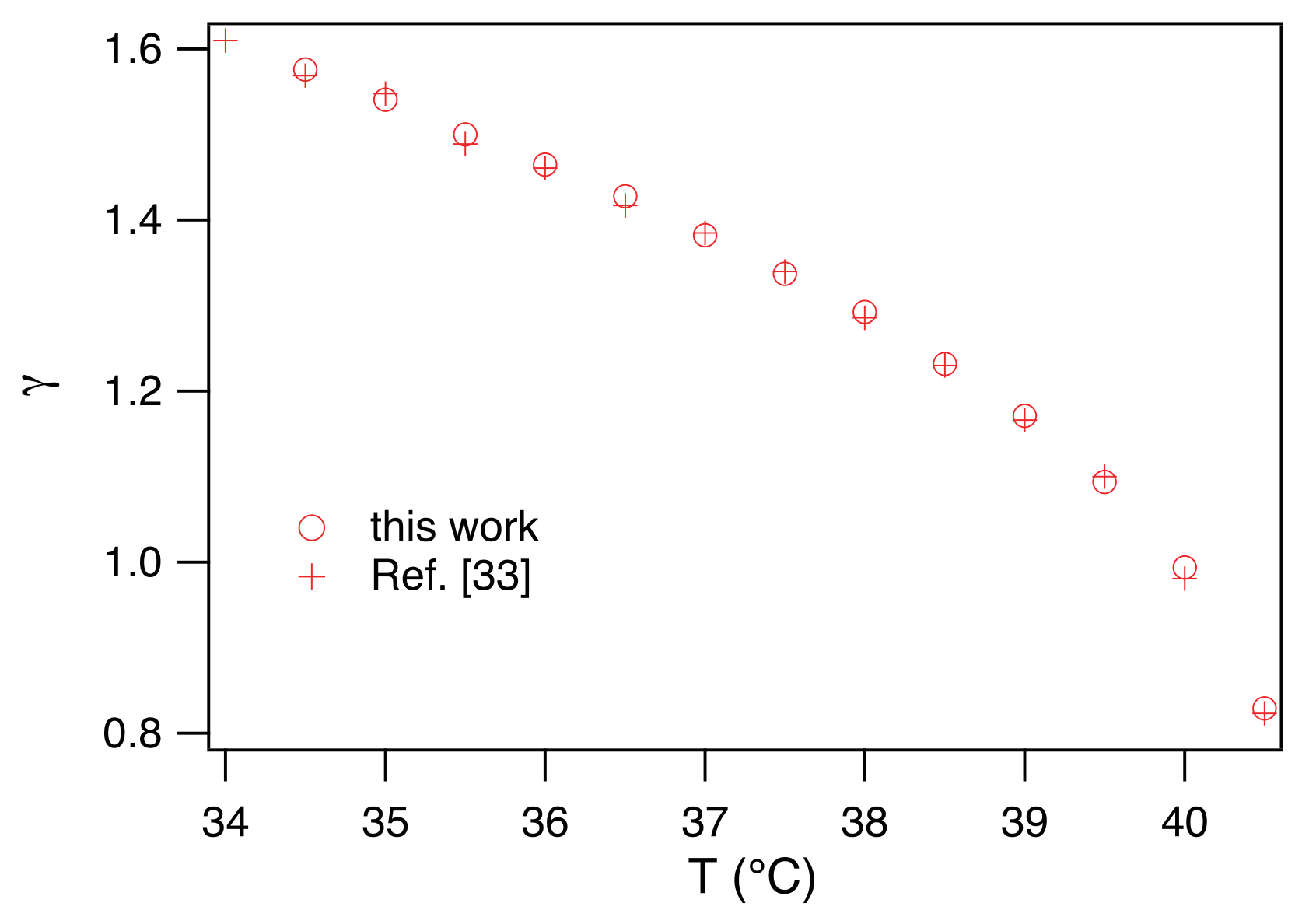
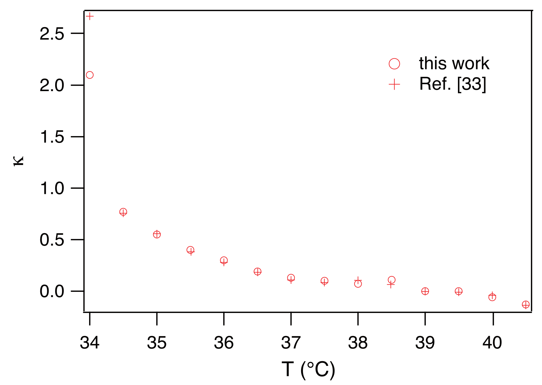
Measurements of ${\epsilon }_{\perp }$ were performed using a planar cell of thickness $d=7.5\mathsf{\mu }$m. In that case, only measurements at low voltage, below $V_c$, are possible. In this range of voltage, I observed that the capacitance was perfectly constant, meaning that the pretilt angle was indeed equal to 0. The temperature dependence of ${\epsilon }_{\perp }$ is shown in Figure 3. From these measurements, I calculated $\gamma$ by taking for ${\epsilon }_{\Vert }$ the value ${\epsilon }_{\Vert }\left(0\right)$ measured at low voltage. The values calculated in this limit are in very good agreement with those measured by Morris et al. [33] in a thick planar sample of thickness $d=75\mathsf{\mu }$m (Figure 4).

3.3. Measurement of the Critical Fréedericksz Voltage $V_c$

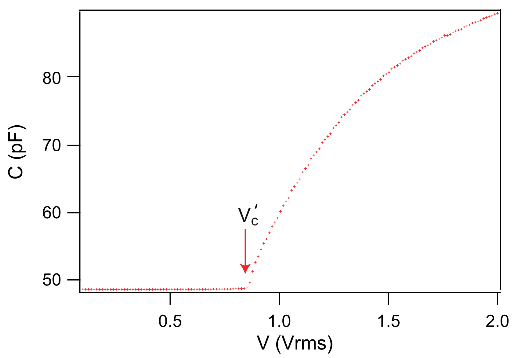
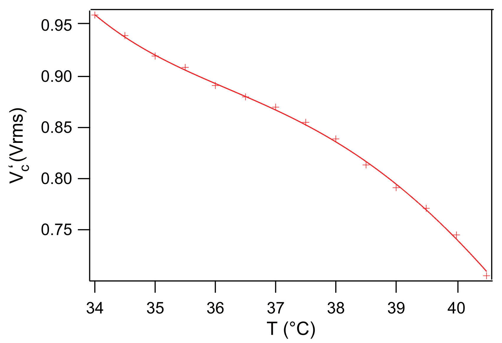
The critical voltage defined in Figure 5 was measured with a 50 $\mathsf{\mu }$m-thick sample. With this thickness, the measured voltage $V_c^{\prime }$ is equal to $V_c$ to better than 1% if $L<0.25\mathsf{\mu }$m, a condition well fulfilled experimentally in my experiments at all temperatures, as I will check a posteriori (see Figure 11a below). The measurements were performed by increasing very slowly the voltage by increments of 10 mV with a time interval of 30 s between each increment. A capacitance curve is shown in Figure 5. This curve shows that the measured capacitance is perfectly constant below the onset of instability, showing that there is no pretilt in my sample. The measured critical voltage as a function of temperature is shown in Figure 6.

3.4. Measurements of the Extrapolation Length L

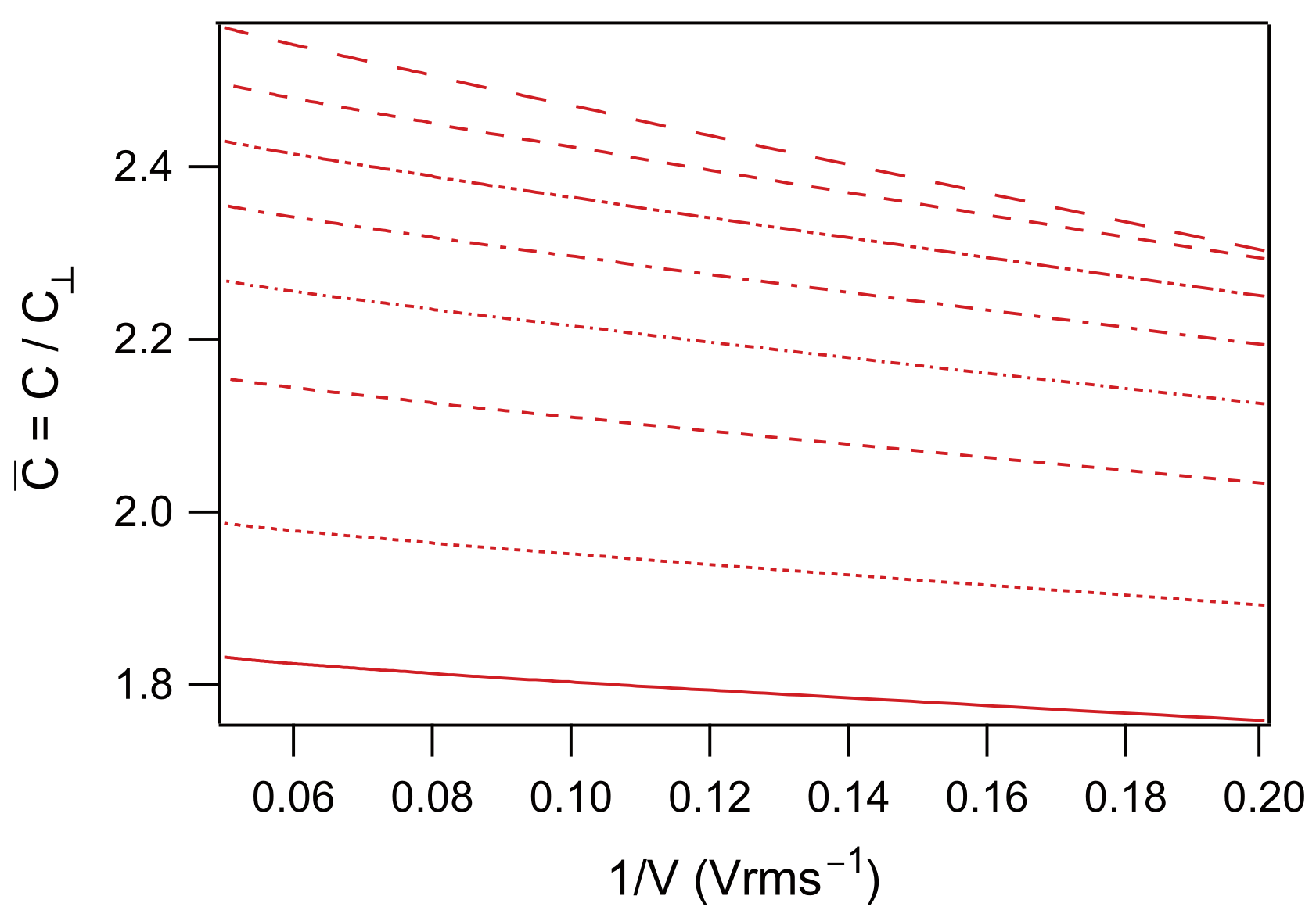
As the anchoring is expected to be strong with Brilliant Yellow, a pretty thin sample must be used in order for the tilt angle $\theta$ on the plates to deviate from 0 in a measurable way under the action of the electric field. For this reason, I used a $8.3\mathsf{\mu }$m-thick sample and I measured the capacitance between 0.1 V and 0.5 Vrms to obtain $C_{\perp }$ and between 5 and 20 Vrms to measure the extrapolation length L. At a voltage V = 5 Vrms the condition $V>6V_c$ is always satisfied, so the basic Equations (4) and (5) apply. Typical curves $\overline{C}\left(\overline{V}\right)$ measured between 5 and 20 Vrms are shown in Figure 7. These curves are almost linear, suggesting that the angle $\theta$ remains small and Equation (6) applies. In that case, fitting the curves with the linear law $1+{\gamma }_{app}-p\overline{V}$ in any voltage range $(V_1,V_2)$ with $V_1>5$Vrms and $V_2<20$Vrms should allow me to measure L by using the equation

$$\frac{L}{d}=\frac{{\gamma }_{app}-\gamma }{2\gamma (1+{\gamma }_{app})},$$

(7)

derived from Equation (6) and the value of $\gamma$ given in Figure 4. To test this method, I fitted the curves within different intervals of voltage $(V_1,V_2)$. For each fit, I calculated L and $V_{\max }$ by using the formula given in the introduction to check whether $V_2<V_{\max }$ in order that the model applies. In principe, all the measurements should coincide if the model applies. In practice, it is not at all the case, the value of L crucially depending on the choice of the interval $(V_1,V_2)$, even when the model is a priori valid, as the reader can see in

Table 1. Value of L obtained from fitting in the voltage range $(V_1,V_2)$.

Voltage Range $({\mathit{V}}_1,{\mathit{V}}_2)$	Fitted Value of L (in $\mathsf{\mu }$m)	${\mathit{V}}_2$	Is the Model Applicable?
(5 V, 9 V)	0.0104	29 V	Yes
(5 V, 13 V)	0.0144	21 V	Yes
(5 V, 17 V)	0.0178	17 V	Yes
(5 V, 20 V)	0.0202	15 V	No

obtained by fitting the curve at $T=35{}^{\circ }$C. To summarize, I met the same difficulties as Nastishin et al. when they used the YvS or RV method. In a similar way, I also noted that the larger $V_2$, the larger the value of L found from the linear fit.

In their paper, Nastishin et al. [17] suggest that this problem could be due to inhomogeneities of the anchoring conditions. I do not share that view, at least in my experiments, and suggest that the problem is rather due to the approximations performed by using Equation (6) with ${\epsilon }_{\Vert }$ constant.

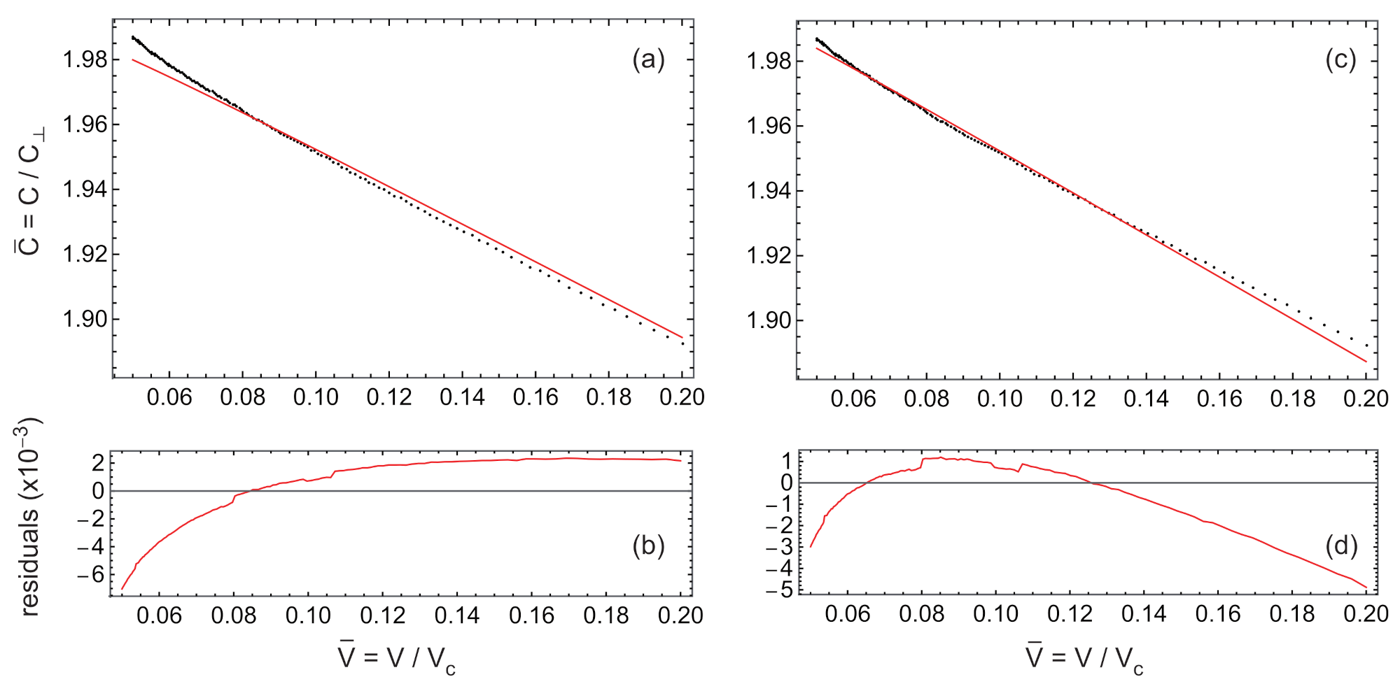
For this reason, I tried in a first attempt to fit my experimental curves with the full Equations (4) and (5), while still keeping ${\epsilon }_{\Vert }$ constant, equal to ${\epsilon }_{\Vert }\left(0\right)$. In that case, there are two fit parameters: the elastic anisotropy $\kappa$ that essentially fixes the slope of the curve and the ratio $L/d$ that fixes the "height" of the curve. Surprisingly, I noted that it was not possible to fit correctly my experimental curves at large voltages even with the full equations. The graphical comparison between the experimental curve and the calculated ones for two particular values of $\kappa$ is shown in Figure 8. For each fit, the root-mean-square deviation between the experimental curve and the fit curve is minimized as a function of L. In this example, $T=40{}^{\circ }$C and the expected value for $\kappa$ at this temperature is close to −0.08 according to previous measurements performed in thick samples at low voltage when the anchoring energy can be assumed to be infinite [33] or by using a full-optical method [24]. For this reason, I performed the first fit (Figure 8a,b) with this value and found $L=0.037\mathsf{\mu }$m. In that case, the slope of the theoretical curve is correct at low voltage (below 10 Vrms), but the model fails to reproduce the increase in the capacitance at large voltage, above 10 V. Increasing the value of $\kappa$ enables better fitting the behavior at large voltage but, this time, the slope of the theoretical curve is clearly too large at low voltage. The best global fit is obtained by taking $\kappa =0.72$ (which is very different from the expected value −0.08) and $L=0.05\mathsf{\mu }$m and is shown in Figure 8c,d. This analysis shows the impossibility to reasonably fit the experimental curves in the whole range of voltages used experimentally. Something is clearly missing in the model.

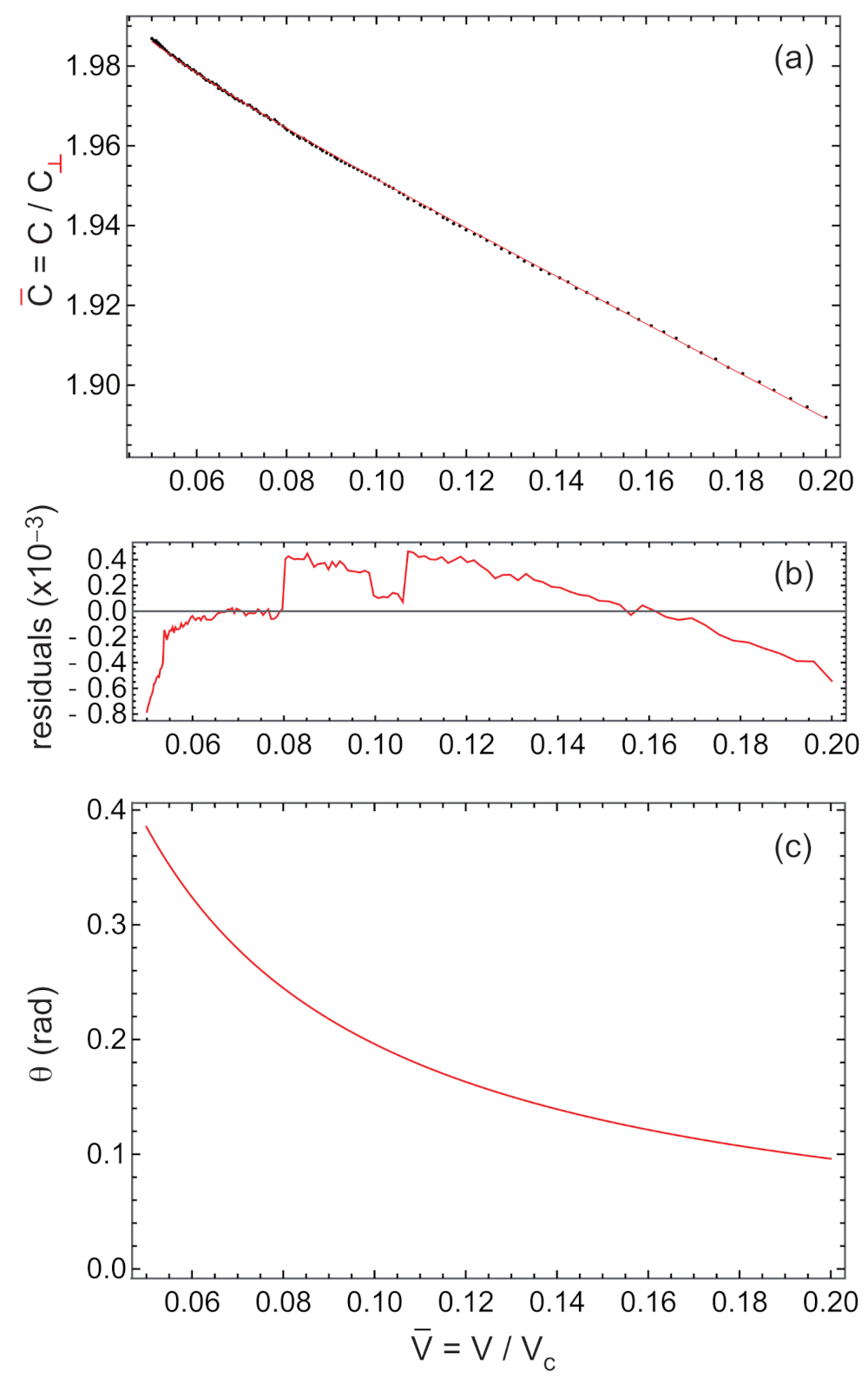
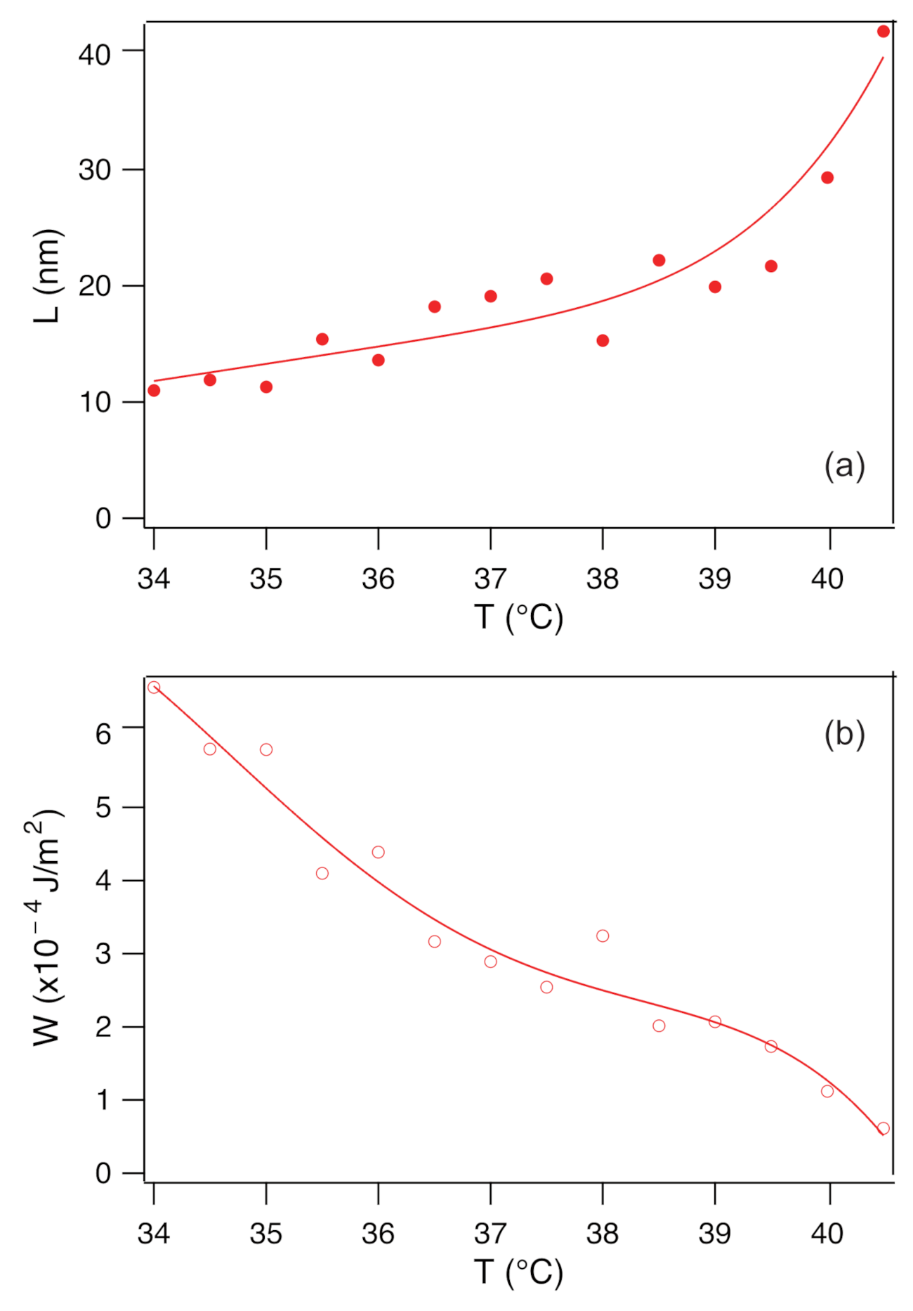
For this reason, I tried to fit again my curves by taking into account the dependence with the electric field of the dielectric constant ${\epsilon }_{\Vert }$ measured previously in homeotropic samples (Figure 2). This correction is here justified because the sample is almost homeotropic between 5 and 20 Vrms and was already taken into account by Murauski et al. [27] in a similar problem. With the aid of Mathematica 12, I realized that it was possible to considerably improve the quality of the fits. The example of the same curve as before measured at $T=40{}^{\circ }$C is shown in Figure 9. In this case the best fit as a function of $\kappa$ and L of the whole curve gives $\kappa =-0.08$ and $L=0.0293\mathsf{\mu }$m with a residual always less than $5\times {10}^{-4}$ in spite of the fact that angle $\theta$ is pretty large at this temperature at large voltage. This is ten times better than before, as we can see by comparing the residuals of the fits shown in Figure 8 and Figure 9. In addition, the value of $\kappa$ found here is in very good agreement with that found by Morris et al. [33] or by us (myself and J. Colombier) by using a full-optical method [24]. This good agreement was confirmed at all the other temperatures, showing the importance of taking into account the electric field dependence of ${\epsilon }_{\Vert }$ in the fit of the experimental curves at large electric field. The values of $\kappa$ and L obtained this way are shown in Figure 10 and Figure 11a, respectively. Finally, the last graph in Figure 11b shows the temperature dependence of the anchoring energy W calculated by using the value of $K_1$ deduced from our measurements of $V_c$ by taking ${\epsilon }_a={\epsilon }_{\Vert }\left(0\right)-{\epsilon }_{\perp }$. The graph shows that W decreases when the temperature increases and approaches the melting temperature. By contrast, no divergence is observed in the vicinity of the smectic A phase, contrary to what is observed for the bend and twist elastic constants.

4. Role of Flexoelectric Effects

As we can see in Figure 9a, the fit of the capacitance curve is not perfect. For this reason, I tried to improve it by introducing a flexoelectric contribution following a procedure detailed in a previous publication [24]. I found that the best fits were systematically obtained by taking the bulk flexoelectric coefficient $e^{🟉}=0$ [34]. That means flexoelectric effects are completely screened out by the ions in the present experiments. This result was expected because the Debye length $L_D$ in our samples is of the order of 50 nm, which is indeed much smaller than the sample thickness [35,36,37]. This value was obtained from the measurement of the charge relaxation frequency $f_c\approx 500$Hz by using formula ${\lambda }_D\approx \sqrt{\frac{D}{2\pi f_c}}$ [38] and by taking $D=10\mathsf{\mu }$m${}^2$/s for typical value of the diffusion coefficient of ions in 8CB [39].

5. About the Rapini–Papoular Form of the Anchoring Energy

Numerous experiments suggest that the actual anchoring potential shifts from the Rapini–Papoular form at a large tilt angle [2,3,15,40,41,42,43]. Another possibility to improve the quality of the fits is to modify the form of the anchoring potential. Several solutions have been proposed in the literature. One of them consists of replacing the sinus in the Rapini–Papoular potential by an elliptic sinus [42]. This function is complicated to work with and I did not use it. Another much simpler and very classical solution is to add a term in ${sin}^4\theta$ to the potential [15,40,41,44,45]. In that case, the anchoring potential can be written in the form

$$W\left(\theta \right)=\frac{1}{2}W\frac{{sin}^2\theta +A{sin}^4\theta }{1+A},$$

(8)

and the torque Equation (5) becomes

$$\frac{1+2A{sin}^2\theta }{1+A}sin\theta =\sqrt{\frac{1+\kappa {sin}^2\theta }{1+\gamma {sin}^2\theta }}\frac{\pi }{\sqrt{1+\gamma }}\frac{L}{d}\frac{V}{V_c}\frac{C}{C_{\perp }}.$$

(9)

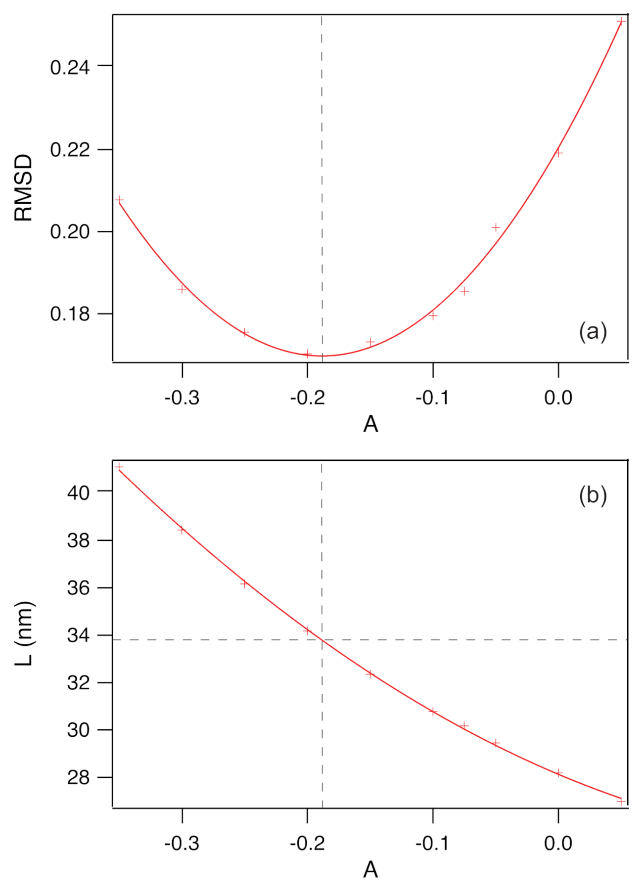
To test the pertinency of this correction, I fitted the capacitance curve measured at $40{}^{\circ }$C with this new potential by using the value of $\kappa$ previously found and I minimized the root-mean-square deviation (RMSD) between the experimental curve and the theoretical curve obtained by solving numerically with Mathematica Equations (4) and (9). In practice, the RMSD was minimized as a function of $L=K_1/W$ for different values of A. The result is shown in Figure 12. This graph shows that the RMSD passes through a minimum for $A=-0.188$ and $L=33.8$nm.

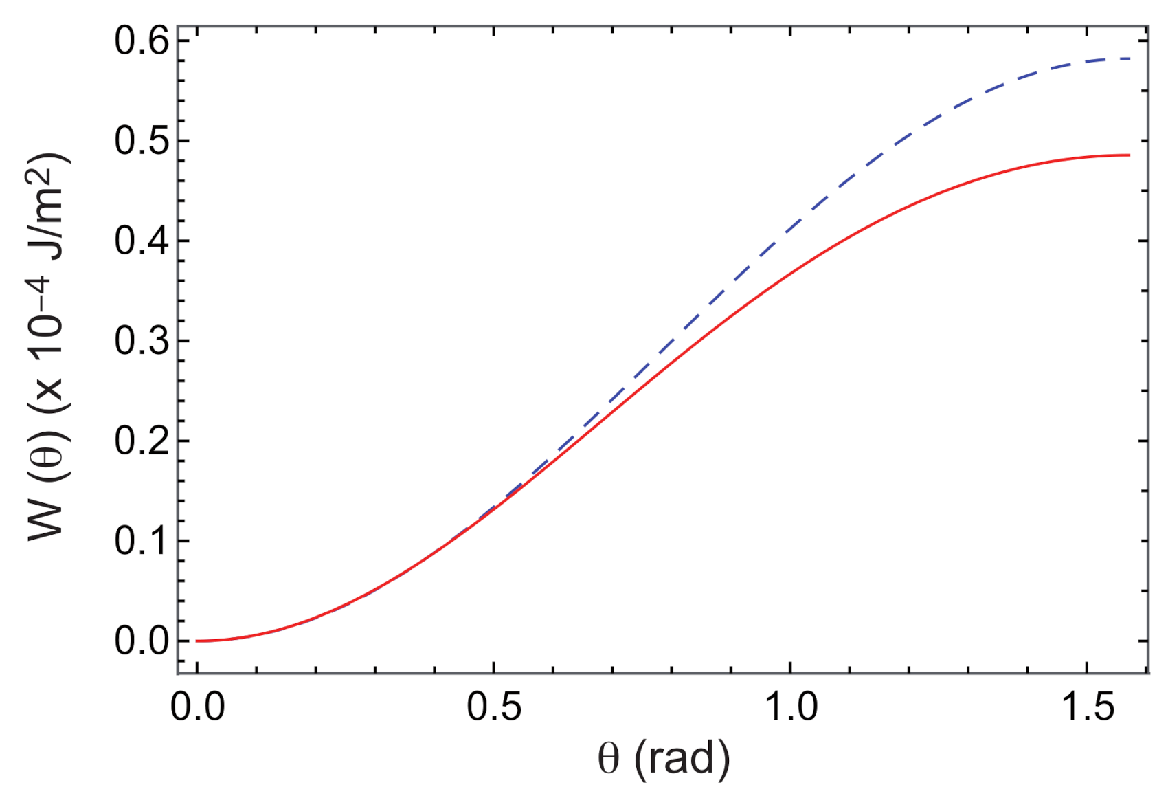
This calculation shows that the actual potential is different from the Rapini–Papoular potential and flattens when $\theta \to \pi /2$. Such a tendency was already observed experimentally [14,15]. The difference between this potential and the one of the Rapini–Papoular form is nonetheless very small in the range of angles $\theta$ probed in this experiment ($\theta <0.4$rad according to Figure 9c as the reader can see in Figure 13). This explains why the RMSD does not change much as a function of A in Figure 12a. In practice, it would be interesting to use larger field to test the relevance of this correction to the Rapini–Papoular potential. I also mention that this value of A is compatible with the second order character of the Fréedericksz transition observed here as shown by Guochen et al. [46].

6. Conclusions

This analysis confirms that neglecting the dependence on the electric field of the dielectric constant ${\epsilon }_{\Vert }$ in the analysis of the capacitance curves at high voltage may be dangerous and lead to wrong values of the extrapolation length [27]. This effect is clearly at the origin of the breakdown of the analysis of the capacitance curves with the linear law given in Equation (6) which gives values of L strongly dependent on the voltage range used to fit the data when ${\epsilon }_{\Vert }$ is taken as a constant. I notice that the behavior observed in my analysis, namely a value L that systematically decreases when the fits are performed at large voltages, is the same as the one reported by Nastishin et al. [5] by using the YvS or the RV techniques. This result suggests that the problems faced by these authors are due to the variation with the electric field of the dielectric constant ${\epsilon }_{\Vert }$ rather than to anchoring inhomogeneities in the samples. This effect should be particularly important in LC such as 8CB which is composed of molecules with a strong electric dipole moment.

To measure the extrapolation length, I thus propose a new procedure that is more general than the one proposed by Murauski et al. [27] and perhaps easier to implement. This procedure consists of solving directly the full Equations (3) and (4) governing the problem, which is much more rigorous than using the approximate Equation (5) as these authors do. Indeed, this equation assumes that the anchoring angle $\theta$ is small, typically less than 0.2 rad, which is a strong limitation at large field (I also mention here that Formula (2) in [27] is wrong and must be read $B=\sqrt{\frac{(1-y_p)(1+\kappa y_p)}{1+\gamma y_p}}$). Another advantage of my method is that it simultaneously gives the values of the two dielectric constants and of the elastic constants $K_1$ and $K_3$. My method can also be used to test the shape of the anchoring potential, as it does not assume that the anchoring potential is of the Rapini–Papoular form. This method is also easy to implement because the Equations (3) and (4) are easily solved numerically, for instance with Mathematica.

Last but not least, this method can also be generalized to the case of samples with a pretilt angle, as the ones obtained by using a rubbed polymer. In that case, it is sufficient to replace $\theta$ by $\theta -{\theta }_a$ in the l.h.s. of Equation (5) where ${\theta }_a$ is the pretilt angle. Note also that the measurement of $V_c$ must be performed with a thick parallel planar sample (the reason for this is explained in [24]). This is important because badly measuring $V_c$ changes the slope of the experimental curves $\overline{C}\left(\overline{V}\right)$ and thus the value of $\kappa$. By contrast, the measurements of the extrapolation length must be performed with an antiparallel sample in order for Equations (3) and (4) (or (9)) to apply. This method could also be applied to LC with a negative dielectric anisotropy to measure the polar anchoring energy under homeotropic anchoring.

In the future, it would be interesting to perform experiments at larger field to better test the validity of the Rapini–Papoular form of the anchoring potential. It would also be interesting to compare the values of L and A obtained this way with those obtained, for instance, by measuring the critical voltage $V_c^{\prime }$ in a wedge sample [47] and by using more sophisticated methods such as the one based on spectroscopic ellipsometry [48,49] or the all-optical compensated method of Murauski et al. [14].

References

- Oswald, P.; Pieranski, P. Nematic and Cholesteric Liquid Crystals: Concepts and Physical Properties Illustrated by Experiments; CRC Press: Boca Raton, FL, USA, 2005; pp. 339–366. [Google Scholar]
- Jerome, B. Surface effects and anchoring in liquid crystals. Rep. Prog. Phys. 1991, 54, 391–452. [Google Scholar] [CrossRef]
- Jerome, B. Physical Properties: Surface Alignment. In Handbook of Liquid Crystals: Fundamentals; Demus, D., Goodby, J., Gray, G.W., Spiess, H.-W., Vill, V., Eds.; Wiley Online Library: Hoboken, NJ, USA, 1998; pp. 535–548. [Google Scholar]
- Chen, R.H. Liquid Crystal Displays: Fundamental Physics and Technology; John Wiley & Sons: Hoboken, NJ, USA, 2011. [Google Scholar]
- Nastishin, Y.A.; Polak, R.D.; Shiyanovskii, S.V.; Bodnar, V.H.; Lavrentovich, O.D. Nematic polar anchoring strength measured by electric field techniques. J. Appl. Phys. 1999, 86, 4199–4213. [Google Scholar] [CrossRef] [Green Version]
- Ryschenkow, G.; Kleman, M. Surface defects and structural transitions in very low anchoring energy nematic thin films. J. Chem. Phys. 1976, 64, 404–412. [Google Scholar] [CrossRef]
- Riviere, D.; Levy, Y.; Guyon, E. Determination of anchoring energies from surface tilt angle measurements in a nematic liquid crystal. J. Phys. Lett. Paris 1979, 40, 215–218. [Google Scholar] [CrossRef]
- Barbero, G.; Barberi, R. Critical thickness of a hybrid aligned nematic liquid crystal cell. J. Phys. Paris 1983, 44, 609–616. [Google Scholar] [CrossRef]
- Barbero, G.; Madhusudana, N.V.; Durand, G. Weak anchoring energy and pretilt of a nematic liquid crystal. J. Phys. Lett. Paris 1984, 45, 613–619. [Google Scholar] [CrossRef]
- Marusii, T.Y.; Reznikov, Y.A.; Reshetnyak, V.Y.; Soskin, M.S.; Khizhnyak, A.I. Scattering of light by nematic liquid crystals in cells with a finite energy of the anchoring of the director to the wails. Sov. Phys. JETP 1986, 64, 502–507. [Google Scholar]
- Vilfan, M.; Mertelj, A.; Čopič, M. Dynamic light scattering measurements of azimuthal and zenithal anchoring of nematic liquid crystals. Phys. Rev. E 2002, 65, 041712. [Google Scholar] [CrossRef] [Green Version]
- Vilfan, M.; Čopič, M. Azimuthal and zenithal anchoring of nematic liquid crystals. Phys. Rev. E 2003, 68, 031704. [Google Scholar] [CrossRef] [Green Version]
- Subacius, D.; Pergamenshchik, V.M.; Lavrentovich, O.D. Measurement of polar anchoring coefficient for nematic cell with high pretilt angle. Appl. Phys. Lett. 1995, 67, 214–216. [Google Scholar] [CrossRef] [Green Version]
- Murauski, A.; Chigrinov, V.; Kwok, H.-S. New method for measuring polar anchoring energy of nematic liquid crystals. Liq. Cryst. 2009, 36, 779–786. [Google Scholar] [CrossRef]
- Yokoyama, H.; Van Sprang, H.A. A novel method for determining the anchoring energy function at a nematic liquid crystal-wall interface from director distortions at high fields. J. Appl. Phys. 1985, 57, 4520–4526. [Google Scholar] [CrossRef]
- Rapini, A.; Papoular, M. Distorsion d’une lamelle nématique sous champ magnétique conditions d’ancrage aux parois. J. Phys. Coll. Paris 1968, 30, C4–54. [Google Scholar] [CrossRef]
- Nastishin, Y.A.; Polak, R.D.; Shiyanovskii, S.V.; Lavrentovich, O.D. Determination of nematic polar anchoring from retardation versus voltage measurements. Appl. Phys. Lett. 1999, 75, 202–204. [Google Scholar] [CrossRef] [Green Version]
- Yaroshchuk, O.; Gurumurthy, H.; Chigrinov, V.G.; Kwok, H.S.; Hasebe, H.; Takatsu, H. Photoalignment properties of brilliant yellow dye. In Proceedings of the International Display Workshop, Sapporo, Japan, 5–7 December 2007; pp. 1665–1668. [Google Scholar]
- Chigrinov, V.; Kwok, H.S.; Takada, H.; Takatsu, H. Photo-aligning by azo-dyes: Physics and applications. Liq. Cryst. Today 2005, 14, 1–15. [Google Scholar] [CrossRef]
- Folwill, Y.; Zeitouny, Z.; Lall, J.; Zappe, H. A practical guide to versatile photoalignment of azobenzenes. Liq. Cryst. 2020, 48, 1–11. [Google Scholar] [CrossRef]
- Fréedericksz, V.; Zolina, V. Forces causing the orientation of an anisotropic liquid. Trans. Far. Soc. 1933, 29, 919–930. [Google Scholar] [CrossRef]
- Deuling, H.J. Deformation of nematic liquid crystals in an electric field. Mol. Cryst. Liq. Cryst. 1972, 19, 123–131. [Google Scholar] [CrossRef]
- Gruler, H.; Scheffer, T.J.; Meier, G. Elastic constants of nematic liquid crystals: I. Theory of the normal deformation. Z. Naturforsch. A 1972, 27, 966–976. [Google Scholar] [CrossRef]
- Oswald, P.; Colombier, J. On the measurement of the bend elastic constant in nematic liquid crystals close to the nematic-to-SmA and the nematic-to-NTB phase transitions. Liq. Cryst. 2021. [Google Scholar] [CrossRef]
- Uchida, T.; Takahashi, Y. New method to determine elastic constants of nematic liquid crystal from CV curve. Mol. Cryst. Liq. Cryst. 1981, 72, 133–137. [Google Scholar] [CrossRef]
- Toko, Y.; Akahane, T. Evaluation of pretilt angle and polar anchoring strength of amorphous alignment liquid crystal display from capacitance versus applied voltage measurement. Mol. Cryst. Liq. Cryst. Sect. A 2001, 368, 469–481. [Google Scholar] [CrossRef]
- Murauski, A.; Chigrinov, V.; Muravsky, A.; Yeung, F.S.-Y.; Ho, J.; Kwok, H.-S. Determination of liquid-crystal polar anchoring energy by electrical measurements. Phys. Rev. E 2005, 71, 061707. [Google Scholar] [CrossRef] [Green Version]
- Akiyama, H.; Iimura, Y. New measurement method of polar anchoring energy of nematic liquid crystals. Mol. Cryst. Liq. Cryst. Sect. A 2000, 350, 67–77. [Google Scholar] [CrossRef]
- Wang, J.; West, J.; McGinty, C.; Bryant, D.; Finnemeyer, V.; Reich, R.; Berry, S.; Clark, H.; Yaroshchuk, O.; Bos, P. Effects of Humidity and Surface on Photoalignment of Brilliant Yellow. Liq. Cryst. 2017, 44, 863–872. [Google Scholar] [CrossRef]
- De Gennes, P.-G.; Prost, J. The Physics of Liquid Crystals; Clarendon Press: Oxford, MS, USA, 1993. [Google Scholar]
- Lelidis, I.; Nobili, M.; Durand, G. Electric-field-induced change of the order parameter in a nematic liquid crystal. Phys. Rev. E 1993, 48, 3818–3821. [Google Scholar] [CrossRef]
- Basappa, G.; Madhusudana, N.V. Effect of a strong electric field on a nematogen: Evidence for polar short range order. Eur. Phys. J. B 1998, 1, 179–187. [Google Scholar] [CrossRef]
- Morris, S.W.; Palffy-Muhoray, P.; Balzarini, D.A. Measurements of the bend and splay elastic constants of octyl-cyanobiphenyl. Mol. Cryst. Liq. Cryst. 1986, 139, 263–280. [Google Scholar] [CrossRef]
- Prost, J.; Pershan, P.S. Flexoelectricity in nematic and smectic-A liquid crystals. J. Appl. Phys. 1976, 47, 2298–2312. [Google Scholar] [CrossRef] [Green Version]
- Dozov, I.; Barbero, G.; Palierne, J.-F.; Durand, G. Nonlocal electric field and large distortions in nematic liquid crystals. EPL 1986, 1, 563–569. [Google Scholar] [CrossRef]
- Palierne, J.-F. Elasticlike contribution of electric origin to the distortion free energy of nematics. Phys. Rev. Lett. 1986, 56, 1160–1162. [Google Scholar] [CrossRef] [PubMed]
- Smith, A.A.T.; Brown, C.V.; Mottram, N.J. Theoretical analysis of the magnetic Fréedericksz transition in the presence of flexoelectricity and ionic contamination. Phys. Rev. E 2007, 75, 041704. [Google Scholar] [CrossRef] [PubMed] [Green Version]
- Bazant, M.Z.; Thornton, K.; Ajdari, A. Diffuse-charge dynamics in electrochemical systems. Phys. Rev. E 2004, 70, 021506. [Google Scholar] [CrossRef] [PubMed] [Green Version]
- Khazimullin, M.V.; Lebedev, Y.A. Influence of dielectric layers on estimates of diffusion coefficients and concentrations of ions from impedance spectroscopy. Phys. Rev. E 2019, 100, 062601. [Google Scholar] [CrossRef] [Green Version]
- Yang, K.H. On the determination of liquid crystal-to-wall anchoring anisotropy by the surface-plasmon polariton technique. J. Appl. Phys. 1982, 53, 6742–6745. [Google Scholar] [CrossRef]
- Yang, K.H.; Rosenblatt, C. Determination of the anisotropic potential at the nematic liquid crystal-to-wall interface. Appl. Phys. Lett. 1983, 43, 62–64. [Google Scholar] [CrossRef]
- Barnik, M.I.; Blinov, L.M.; Korkishko, T.V.; Umansky, B.A.; Chigrinov, V.G. Investigation of NLC director orientational deformations in electric field for different boundary conditions. Mol. Cryst. Liq. Cryst. 1983, 99, 53–79. [Google Scholar] [CrossRef]
- Barbero, G.; Madhusudana, N.V.; Palierne, J.-F.; Durand, G. Optical determination of large distortion surface anchoring torques in a nematic liquid crystal. Phys. Lett. A 1984, 103, 385–388. [Google Scholar] [CrossRef]
- Barbero, G.; Durand, G. On the validity of the Rapini-Papoular surface anchoring energy form in nematic liquid crystals. J. Phys. Paris 1986, 47, 2129–2134. [Google Scholar] [CrossRef]
- Alexe-Ionescu, A.L.; Barbero, G.; Gabbasova, Z.; Sayko, G.; Zvezdin, A.K. Stochastic contribution to the anchoring energy: Deviation from the Rapini-Papoular expression. Phys. Rev. E 1994, 49, 5354–5358. [Google Scholar] [CrossRef]
- Guochen, Y.; Jianru, S.; Ying, L. Surface anchoring energy and the first order Fréedericksz transition of a NLC cell. Liq. Cryst. 2000, 27, 875–882. [Google Scholar] [CrossRef]
- Gu, D.-F.; Uran, S.; Rosenblatt, C. A simple and reliable method for measuring the liquid crystal anchoring strength coefficient. Liq. Cryst. 1995, 19, 427–431. [Google Scholar] [CrossRef]
- Hirosawa, I. Method of characterizing rubbed polyimide film for liquid crystal display devices using reflection ellipsometry. Jap. J. Appl. Phys. 1996, 35, 5873. [Google Scholar] [CrossRef]
- Marino, A.; Tkachenko, V.; Santamato, E.; Bennis, N.; Quintana, X.; Otón, J.M.; Abbate, G. Measuring liquid crystal anchoring energy strength by spectroscopic ellipsometry. J. Appl. Phys. 2010, 107, 073109. [Google Scholar] [CrossRef]
Figure 1.
Dielectric constant measured in a homeotropic sample as a function of the applied voltage. The crosses are experimental points and the solid line is the best fit to a parabola. C.
Figure 2.
Variation with temperature of the dielectric constant extrapolated at zero voltage (a) and of the fit parameters a and b (b). The solid lines are just guides for the eye.
Figure 3.
Dielectric constant measured below the onset of instability in a planar sample of thickness m.
Figure 4.
Dielectric anisotropy calculated by taking the value of extrapolated at V. The agreement with the measurements of Morris et al. [33] is excellent.
Figure 5.
Capacitance curve measured in a planar sample of thickness m at C.
Figure 6.
Critical Fréedericksz voltage as a function of temperature measured in a planar sample of thickness m. The solid line is just a guide for the eye.
Figure 7.
Reduced capacitance curves measured in a planar sample of thickness m at different temperatures. From top to bottom, and C.
Figure 8.
Capacitance curve measured at C (the dots are the experimental points) and its fits to Equations (4) and (5) (solid lines) calculated by taking and m (a,b) or and m (c,d). Here is assumed to be constant and equal to .
Figure 9.
(a) Capacitance curve measured at C (the dots are the experimental points) and its fit (solid line) obtained by taking into account the variation with electric field of . The best fit is obtained by taking and m. (b) Residuals. (c) Angle on the plates as a function of the voltage.
Figure 10.
Values of obtained from the fit of the capacitance curves shown in Figure 7 by taken into account the electric field variation of . The agreement with the values given by Morris et al. is excellent.
Figure 11.
(a) Values of L obtained from the fit of the capacitance curves shown in Figure 7 by taking into account the electric field variation of . (b) Corresponding values of W. Solid lines are just guides for the eye.
Figure 12.
(a) Root-mean-square deviation (RMSD) between the experimental curve measured at C and the theoretical curve as a function of A. (b) Value of L that minimizes the RMSD as a function of A.
Figure 13.
Comparison between the best Rapini–Papoular potential (blue dashed curve) and the best modified Rapini–Papoular potential (red solid curve). The two potentials are almost indistinguishable below rad, meaning that in our experiment, the Rapini–Papoular potential can be used to fit the data.