A Simple Contrast Matching Rule for OSEM Reconstructed PET Images with Different Time of Flight Resolution

Abstract

Background: Time-of-Flight (TOF) is a leading technological development of Positron Emission Tomography (PET) scanners. It reduces noise at the Maximum-Likelihood solution, depending on the coincidence–timing–resolution (CTR). However, in clinical applications, it is still not clear how to best exploit TOF information, as early stopped reconstructions are generally used. Methods: A contrast-recovery (CR) matching rule for systems with different CTRs and non-TOF systems is theoretically derived and validated using (1) digital simulations of objects with different contrasts and background diameters, (2) realistic phantoms of different sizes acquired on two scanners with different CTRs. Results: With TOF, the CR matching rule prescribes modifying the iterations number by the CTRs ratio. Without TOF, the number of iterations depends on the background dimension. CR matching was confirmed by simulated and experimental data. With TOF, image noise followed the square root of the CTR when the rule was applied on simulated data, while a significant reduction was obtained on phantom data. Without TOF, preserving the CR on larger objects significantly increased the noise. Conclusions: TOF makes PET reconstructions less dependent on background dimensions, thus, improving the quantification robustness. Better CTRs allows performing fewer updates, thus, maintaining accuracy while minimizing noise.

1. Introduction

Time of flight (TOF) positron emission tomography (PET) provides additional information in the acquired data respect to conventional non-TOF PET. On top of the non-TOF information, which is sufficient for image reconstruction, TOF provides a range for the probable position of the annihilation event. This makes the tomographic problem better conditioned resulting in reconstructed images with a higher signal-to-noise ratio (SNR).

This makes the tomographic problem better conditioned and the signal-to-noise ratio (SNR) higher on reconstructed images. In a TOF system characterized by a coincidence timing resolution (CTR) $\Delta t$, expressed in full width half maximum (FWHM), the TOF “effective diameter” is $D_{eff}\equiv \sqrt{2\pi }\frac{\Delta t}{\sqrt{8ln2}}c/2$. In the central pixel of a uniform circular object of diameter D, at the maximum likelihood solution, TOF is expected to provide a noise reduction of a factor $\sqrt{D/D_{eff}}$ with respect to non-TOF [1].

In clinical setups, PET images are conventionally reconstructed with Maximum Likelihood Expectation Maximization (MLEM) [2], often used in combination with the ordered subset acceleration, in the so-called OSEM algorithm [3]. In MLEM and OSEM, the signal converges with iterations, which are, however, also characterized by a noise augment. Good SNR images are, therefore, obtained by stopping MLEM and OSEM at early iterations (early stopping rules).

It has already been observed that TOF increases the MLEM convergence speed; therefore, at matched numbers of iterations, both the signal and noise are higher with TOF than without [4,5]. To improve the SNR respect to non-TOF, a lower number of iterations is, therefore, generally recommended with TOF [6]. Empirical stopping rules were derived on patient and phantom data by matching non-TOF noise, thus, obtaining a better contrast or by matching the non-TOF contrast and, thus, maintaining a lower noise.

In [7], as an example, the standard deviation between neighbouring voxels in a liver region of interest (ROI) was considered as a noise measure for noise matching. In other works, the contrast recovery on phantom data was used for contrast matching. These empirical rules depend on the patient/phantom characteristics and on the ROI positioning. Contrast recovery is known to depend on many factors, including the background composition.

The aim of this study is to theoretically derive and experimentally validate a contrast matching stopping rule for TOF data with different CTRs that is able to guarantee contrast matching for the most critical signals and noise reduction. A theoretical rule of this kind is especially important in the context of the release of new TOF-PET systems, with a CTR as low as 210 ps [8].

This paper is structured as follows. After notations and conventions, in Section 2 we analyze the convergence speed of the signal and noise in TOF and non-TOF MLEM and propose an optimal contrast matching stopping rule for scanners with different CTRs. In Section 3 and Section 4 computer simulations and phantom measurements for theory validation are presented.

Notations and Conventions

We indicate with $\lambda$ image voxel activity values, with y sinogram counts, and with $c_{i,j}$ the probability that a photon pair emitted from pixel j is recorded in the sinogram bin i. We use k to indicate the iteration number, using it as a superscript when referring to the estimate of a parameter at the k-th iteration. To avoid confusion with exponentiation, we indicate the latter with parenthesis; e.g., ${\lambda }^k$ is the estimate of $\lambda$ at the k-th iteration, while ${\left(\alpha \right)}^k$ is the k-th power of $\alpha$. The forward projection operator is indicated in component notation as $y_i={\sum }_j{c}_{i,j}{\lambda }_j$, and in matrix notation as $y=H\left[\lambda \right]$, while the backprojector is indicated with $H^T$.

We define the normalization factor ${\eta }_j={\sum }_i{c}_{i,j}$. Matrix multiplications will be highlighted by the use of square brackets (e.g., $y=H\left[\lambda \right]$), while element-wise multiplications will be identified by the Hadamard product “○”. Therefore, the forward projection of the element-wise multiplication between $\lambda$ and a matrix $\delta$ will be written as $H\left[\lambda ○ \delta \right]$. Element-wise divisions are written as standard fractions. Throughout the paper, we will not use resolution modelling within the H operators. Point spread function modelling makes unconstrained MLEM reconstruction undetermined at high frequencies [9]; therefore, studying the convergence of both signal and noise at those frequencies is not possible, as it is dependent on the specific implementation.

2. Theory

2.1. Objects Convergence

We start by analysing the MLEM convergence proprieties. In PET reconstruction, the tomographic problem is the minimization of the negative likelihood

$${\lambda }^{*}=arg\underset{\lambda }{min}\sum _i\overline{y_i}-y_{i}ln\overline{y_i}$$

(1)

with $\overline{y_i}={\sum }_j{c}_{i,j}{\lambda }_j$ as the expected number of counts in each sinogram bin, given the current image estimate $\lambda$. The update equation is

$${\lambda }_j^{k+1}=\frac{{\lambda }_j^k}{{\eta }_j}\sum _i{c}_{i,j}\frac{y_i}{\overline{y_i}}$$

(2)

It has been shown that MLEM can be also written as a gradient descent algorithm, which is expected to converge linearly with a unitary step size and a diagonal preconditioner equal to the current image estimate divided by the normalization matrix [10].

If we look at Equation (2) as ${\lambda }_j^{k+1}=f_j\left({\lambda }^k\right)$, we can compute the Taylor expansion around the solution ${\lambda }^{*}$, ${\lambda }_j^{k+1}\approx {\lambda }_j^{*}+{\sum }_{\xi }\frac{\partial {\lambda }_j^{k+1}}{\partial {\lambda }_{\xi }}\left({\lambda }_{\xi }^k-{\lambda }_{\xi }^{*}\right)$ The derivative of ${\lambda }_j^{k+1}$ against ${\lambda }_{\xi }^k$, considering that $\frac{\partial \overline{y_i}}{\partial {\lambda }_{\xi }}=c_{i,\xi }$, is

$$\frac{\partial {\lambda }_j^{k+1}}{\partial {\lambda }_{\xi }^k}=\frac{{\delta }_{j,\xi }}{{\eta }_j}\sum _i{c}_{i,j}\frac{y_i}{{\overline{y_i}}^k}-\frac{{\lambda }_j^k}{{\eta }_j}\sum _i{c}_{i,j}\frac{y_i}{{\left({\overline{y}}_i^k\right)}^2}{c}_{i,\xi }$$

(3)

By substituting in the Taylor expansion around the solution ${\lambda }^{*}$, we obtain

$${\lambda }_j^{k+1}-{\lambda }_j^{*}\approx \sum _{\xi }\left[{\delta }_{j,\xi }\frac{1}{{\eta }_j}\sum _i{c}_{i,j}\frac{y_i}{{\overline{y_i}}^{*}}-\frac{{\lambda }_j^{*}}{{\eta }_j}\sum _i\frac{c_{i,j}{y}_i}{{\left({\overline{y}}_i^{*}\right)}^2}{c}_{i,\xi }\right]\left({\lambda }_{\xi }^k-{\lambda }_{\xi }^{*}\right)$$

(4)

This equation closely mimics that of an algorithm linearly converging. We will prove that we are able to estimate a linear convergence rate ${\alpha }_j=\frac{∥{\lambda }_j^{k+1}-{\lambda }_j^{*}∥}{∥{\lambda }_j^k-{\lambda }_j^{*}∥}$ for each pixel for different kinds of signals.

A propriety of MLEM is that, after the first iteration [2],

$$\sum _i{y}_i=\sum _i{\overline{y_i}}^k$$

(5)

We therefore approximate ${\sum }_i{c}_{i,j}{y}_i/\overline{y_i^{*}}\approx {\eta }_j$ and ${\sum }_i{c}_{i,j}\frac{y_i}{{\left(\overline{y_i^{*}}\right)}^2}{c}_{i,\xi }\approx {\sum }_i\frac{c_{i,j}}{\overline{y_i^{*}}}{c}_{i,\xi }$. These two approximations modify Equation (4) to

$${\lambda }_j^{k+1}-{\lambda }_j^{*}\approx \sum _{\xi }\left[{\delta }_{j,\xi }-\frac{{\lambda }_j^{*}}{{\eta }_j}\sum _i\frac{c_{i,j}}{{\overline{y}}_i^{*}}{c}_{i,\xi }\right]\left({\lambda }_{\xi }^k-{\lambda }_{\xi }^{*}\right)=$$

(6)

$$=\left({\lambda }_j^k-{\lambda }_j^{*}\right)-\frac{{\lambda }_j^{*}}{{\eta }_j}\sum _i\frac{c_{i,j}}{{\overline{y}}_i^{*}}\sum _{\xi }{c}_{i,\xi }\left({\lambda }_{\xi }^k-{\lambda }_{\xi }^{*}\right)$$

where ${\lambda }^k$ is the free parameter of the Taylor expansion.

To simplify this expression, we need to compute ${\sum }_{\xi }{c}_{i,\xi }\left({\lambda }_{\xi }^k-{\lambda }_{\xi }^{*}\right)$. Exploiting again the propriety mentioned in Equation (5), we can state that, in uniform large regions, which generally make up the biological background, ${\sum }_{\xi }{c}_{i,\xi }\left({\lambda }_{\xi }^k-{\lambda }_{\xi }^{*}\right)\approx 0$. If, instead, centered around a pixel j there is a signal characterized by a “dimension” d to be recovered, we can model:

$${\lambda }_{\xi }^k-{\lambda }_{\xi }^{*}=\left({\lambda }_j^k-{\lambda }_j^{*}\right)g\left(\frac{x}{d}\right);$$

(7)

where g is a function of the distance x from pixel j to pixel $\xi$, to which it is only required to have a finite integral ${\int }_{-r}^{+r}g\left(x/d\right)dx=\gamma d$, with $\gamma$ as the scale-independent integral value. In general $\gamma <1$ (e.g., only for a step function $\gamma =1$. A smooth function like half a cosine period has $\gamma =2//\pi$). In this model, by approximating a finite forward projection along an LOR with the integral, we have ${\sum }_{\xi }{c}_{i,\xi }\left({\lambda }_{\xi }^k-{\lambda }_{\xi }^{*}\right)\approx \gamma d\left({\lambda }_j^k-{\lambda }_j^{*}\right)$. Therefore, Equation (6) becomes

$${\lambda }_j^{k+1}-{\lambda }_j^{*}\approx \left({\lambda }_j^k-{\lambda }_j^{*}\right)\times \left[1-\frac{\gamma }{{\eta }_j}\sum _i\frac{c_{i,j}{\lambda }_j^{*}d}{{\overline{y_i}}^{*}}\right]$$

(8)

where all terms are now independently computed for each pixel. We can estimate a convergence rate ${\alpha }_j$ by dividing both side of the equation by ${\lambda }_j^k-{\lambda }_j^{*}$ and obtaining

$${\alpha }_j\approx 1-\frac{\gamma }{{\eta }_j}\sum _i{c}_{i,j}\frac{c_{i,j}{\lambda }_j^{*}d}{{\sum }_{\zeta }{c}_{i\zeta }{\lambda }_{\zeta }^{*}}$$

(9)

In this equation, it can be seen that the signal convergence depends on its spatial extension and on the fraction of counts due to the signal over all the LORs.

This equation holds for a generic signal in a generic background. For an exemplary setup, the forward projections can be analytically computed further simplifying this expression.

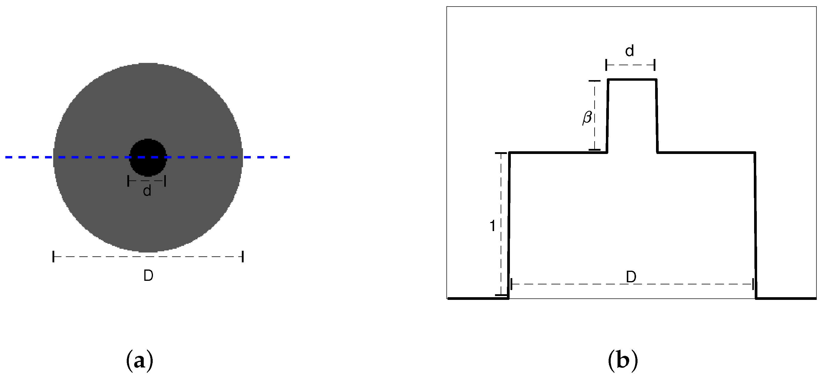
Let us assume an image composed of a background circle of diameter D with a smaller concentric circle of diameter d and activity ratio $\beta$, as shown in Figure 1. In the central pixel j, $c_{i,j}{\lambda }_j^{*}=\varphi \beta$ for every LOR i crossing pixel j, with $\varphi$ a constant accounting for the direct relation between a pixel activity and the expected counts. Since ${\sum }_{\zeta }{c}_{i\zeta }{\lambda }_{\zeta }^{*}=\varphi \left[D+\left(\beta -1\right)\right]d$, we can further simplify Equation (9) as

$${\alpha }_j=1-\gamma \frac{d\beta }{D+(\beta -1)d}$$

(10)

With TOF, the same equation holds with $D_{eff}$ in place of D, if $D_{eff}<D$. A few things can be noticed:

• With increasing the signal to background contrast $\beta$, the convergence is faster.
• With increasing object size d, the convergence speed also increases.
• If an object is totally cold, i.e., $\beta =0$, the convergence rate approaches 1. This makes cold object convergence extremely slow.
• Without TOF, the convergence speed decreases with background diameter D. With TOF, instead, convergence does not depend on D (for $D>D_{eff}$).
• With TOF, convergence depends on $D_{eff}$; if $d\approx D_{eff}$ convergence is almost instantaneous.
• For the full reconstruction of a circle, not only low frequency components need to converge but also high frequency components. Each frequency converges according to the same equation by replacing d with $\frac{1}{f}$.

Equation (10) with $\beta =1$ and $d=\frac{1}{f}$ can also describe the convergence of background noise frequencies f. Without TOF, the larger the background diameter D, the slower the noise converges. This implies that, without TOF, a fixed stopping rule produces comparable noise levels on reconstructed images, even if the noise at convergence is higher for larger objects. For higher noise frequencies, $\alpha \to 1$. Since for a number $\epsilon$ close to 1 ${\left(1+\epsilon \right)}^k\approx 1+k\times \epsilon$, it can be said that high frequency noise increases almost linearly with iterations in early stopped reconstructions.

2.2. Contribution of Attenuation, Random and Scattered Coincidences

2.2.1. Attenuation

Using a notation where $c_{i,j}$ represents the total probability of a photon emitted from the pixel j to be detected in detector i, the attenuation is naturally accounted for in all the previous equations, without any modification.

2.2.2. Random and Scattered Coincidences

In presence of an expected rate of random coincidences r and of scattered coincidences s, Equation (2) becomes

$${\lambda }_j^{k+1}={\lambda }_j^k/{\eta }_j\sum _i{c}_{i,j}\frac{y_i}{{\sum }_{\xi }{c}_{i,\xi }{\lambda }_{\xi }^k+r_i+s_i}$$

(11)

Therefore, Equation (9) still holds by considering the contribution of scatter and random coincidences to $y_i$.

It can be seen that, the higher is the fraction of random and scattered coincidences, the slower is the convergence rate. In TOF, random coincidences are uniformly distributed over time bins. Pixel convergence is, therefore, influenced not by the whole random amount, but only by the fraction $D_{eff}/FOV$ happening within $D_{eff}$.

TOF greatly reduces the randoms impact on MLEM convergence. On the other side, since the scatter coincidence profile over time bins follows that of emission coincidences [11], the scatter impact on convergence is not reduced with TOF. Furthermore, as the scatter fraction greatly increases with object dimension, the previously observed TOF convergence rate independence from background dimension D is no longer accurate.

2.3. An Optimal Stopping Rule

In this section, we propose a rule to guarantee matched contrast recovery for the exemplary object used to derive Equation (9), which can approximate an oncological lesion in an at least locally uniform background. It is also the same kind of object for which the noise reduction law was derived for PET systems (i.e., the center of a uniform phantom).

In non-TOF PET, two objects with equal contrast $\beta$ and dimension d, positioned in two different backgrounds of dimensions D and $D^{\prime }$, achieve the same convergence level (i.e., the same contrast recovery) when ${\left({\alpha }_j^{\prime }\right)}^{k^{\prime }}={\left({\alpha }_j\right)}^k$; therefore, the MLEM iteration numbers k and $k^{\prime }$ are related by

$$k^{\prime }=k\frac{log{\alpha }_j}{log{\alpha }_j^{\prime }}$$

(12)

Particular attention must be paid to small objects with low contrast where, as previously shown, convergence is the slowest, therefore $\alpha \to 1$. In these conditions $log\left(\alpha \right)\approx \alpha -1$, so

$$k^{\prime }=k\frac{\frac{-d\beta }{D+\left(\beta -1\right)d}}{\frac{-d\beta }{D^{\prime }+\left(\beta -1\right)d}}\approx k\frac{D^{\prime }}{D}$$

(13)

where the last step assumes that $D\gg \left(\beta -1\right)d$, which is always the case when $\alpha \to 1$. This equation shows that contrast recovery for small and low contrasted objects depends very strongly on the background, i.e., a fixed number of iterations cannot provide consistent contrasts for these targets, if positioned in different patients/body districts/phantoms. For larger and more contrasted objects Equation (12) still holds, but the two approximations are no longer valid and the convergence speed is faster. Therefore, the rule proposed in Equation (13) provides higher contrast recovery than desired.

Rule (13) is easily extendable to TOF-PET. Given two TOF-PET scanners with effective diameters $D_{eff}$ and $D_{eff}^{\prime }$, similar contrast recoveries for similar small and low contrast objects are achieved when

$$k^{\prime }=k\frac{D_{eff}^{\prime }}{D_{eff}}$$

(14)

or, in terms of CTR, when

$$k^{\prime }=k\frac{\Delta t^{\prime }}{\Delta t}$$

(15)

This simple stopping rule in TOF no longer depends on background characteristics. Therefore, it can be used to obtain similar contrast recovery levels for similar objects on TOF scanners with different CTRs. It is also possible to apply this rule to the non-TOF case, using Equation (13), but this would imply a different number of iterations for each patient and bed position, according to the “diameter” of that body region.

Due to considerations in Section 2.2, rule (14) completely removes the dependence on object background only when the fraction of scatter and random counts is constant. With good CTR, the impact of randoms is expected to be negligible. The scatter fraction might instead partially change between different subjects/objects. Therefore, we expect that when the rule is applied on real data, an approximate matching is observed.

3. Simulations

3.1. Methods

3.1.1. Simulation and Reconstruction Programs Description

Simulations to validate the proposed stopping rules were performed in an idealized setting to minimize computation time. Matched distance-driven projectors and backprojectors were used [12], simulating a single slice of a scanner with a 829 mm ring diameter, and 4.3 mm crystals. The same projectors were used for image reconstruction. Images were generated at high resolution (1.36 mm pixel size), smoothed with a 4.5 mm FWHM Gaussian kernel, then forward projected.

Two additive corrections were simulated: a uniform background in sinogram space (representing random coincidences) and a multi-kernel convolution of the true sinogram (to represent scatter coincidences). For every true coincidences $0.9$ random and $0.5$ scattered coincidences were added. After forward projection, Poisson noise was simulated. Sinograms were then reconstructed in a 512 mm FOV, using 2 mm pixels and 200 MLEM iterations, without OS acceleration. Reconstructions were initialized with a unitary circle as large as the FOV.

3.1.2. Phantom

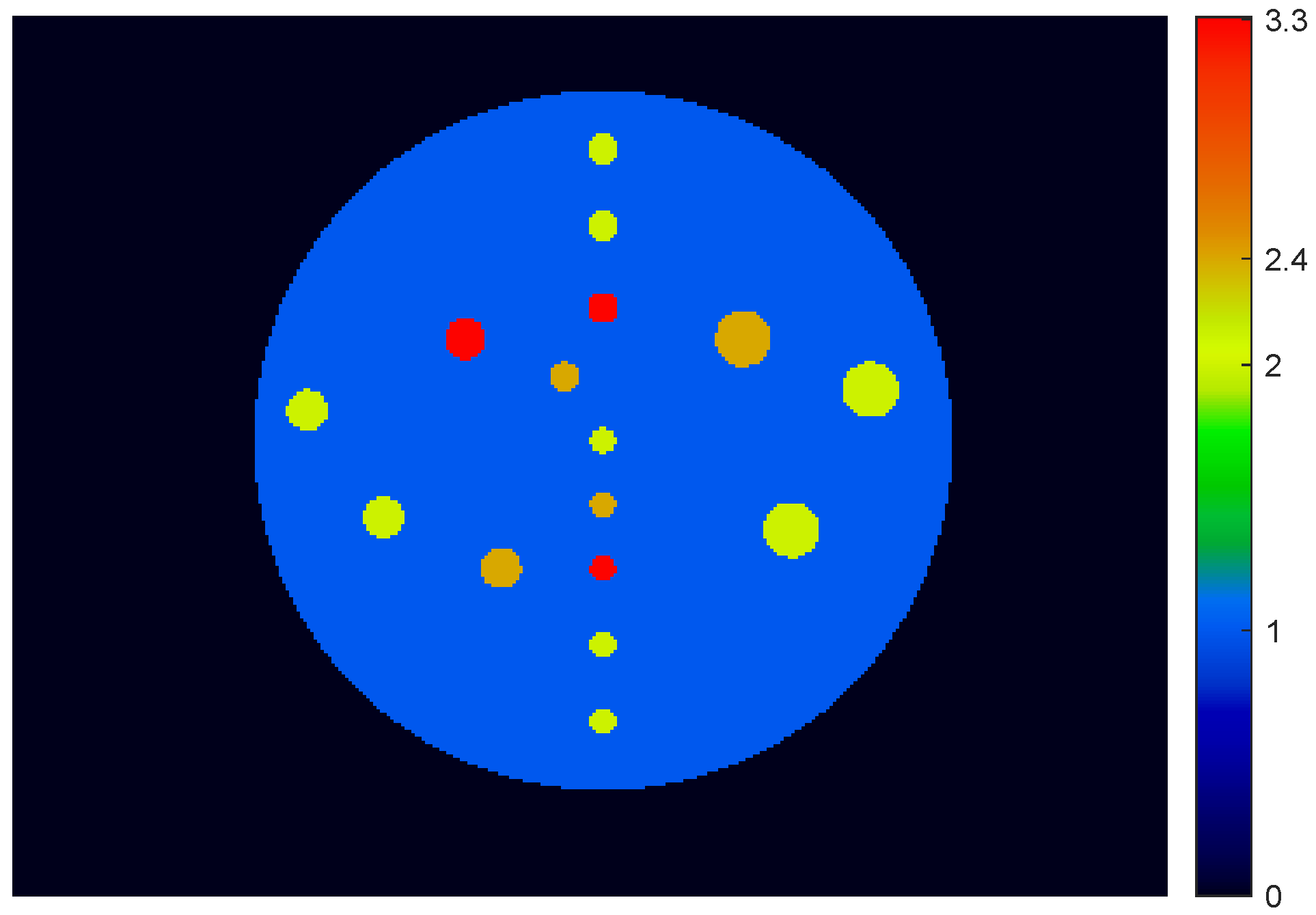
Circular backgrounds with the diameters 275, 320, and 440 mm, each containing 16 circular targets of interest, were simulated. Targets had 10, 12, 16, and 22 mm diameters and $\beta =2.0,2.4$, and $3.3$ contrasts relative to the background. Uniform water attenuation was simulated in all the phantom area. CTRs of 250, 400, 550, and 750 ps were used. For each combination of background diameter and CTR, 12 independent noise realizations were simulated. The phantom is shown in Figure 2.

3.1.3. Image Analysis

The reconstructed images were analyzed using contrast recovery and background variability, similarly to what is done in NEMA image quality analysis. Target contrast recovery was computed as

$$CR=\frac{C_{meas}-1}{C_{true}-1}$$

(16)

where $C_{true}$ is the simulated contrast and $C_{meas}$ is the measured contrast, obtained as the ratio between the activity measured in a circular ROI of the known true diameter positioned on the target and the average activity measured in multiple background ROIs. Contrast convergence with iterations was measured in all the explored $\beta$ and D conditions for non-TOF PET and in all the $\beta$, D and CTR conditions for TOF PET.

We then concentrated on the contrast $\beta =2.0$, characterized by the slowest convergence rate. We initially assessed contrast recovery at 50 MLEM updates both in non-TOF and in TOF simulations. Then, to validate the proposed rule, we took, as reference, 50 MLEM updates of the highest CTR TOF simulation and measured, in both non-TOF and TOF data in all the D and CTR conditions, the contrast recovery at the update number provided by the rule.

Noise was quantified as background variability by defining 21 positions in the background and computing the activity a in ROIs with 1 pixel (2 mm), and 3, 5, and 7 mm diameters. Background variability was then defined as

$$B{V}_{ROI}=\frac{\mathrm{std}\left(a\right)}{\mathrm{mean}\left(a\right)}.$$

(17)

3.2. Results

3.2.1. Contrast Recovery

In Figure 3, the contrast recovery convergence with MLEM updates is shown for TOF data with $CTR=750\mathrm{ps}$ and background diameter $D=275\mathrm{mm}$. It can be appreciate how, with TOF, convergence speed does not depend on the object position within the background and how higher $\beta$ values result in faster convergence, as predicted by Equation (10).

Contrast recovery values at 50 updates for contrast activity $\beta =2.0$ are shown in

Table 1. Contrast recovery at 50 updates for the 10 mm sphere with $\beta =2.0$ contrast, as a function of CTR and background diameter. Values reported as mean ± one standard error.

Background:	275 mm	320 mm	440 mm
CTR [ps]	CR [%]	CR [%]	CR [%]
Non-TOF	$37.0\pm 1.5$	$33.5\pm 1.8$	$20.3\pm 2.7$
750	$59.1\pm 1.8$	$62.9\pm 2.8$	$56.4\pm 3.5$
550	$67.1\pm 2.4$	$65.5\pm 1.9$	$67.2\pm 4.9$
400	$71.3\pm 1.6$	$70.6\pm 1.8$	$72.1\pm 3.9$
250	$73.8\pm 1.4$	$76.5\pm 2.2$	$75.5\pm 3.9$

for non-TOF and TOF conditions corresponding to different D and CTR values. As expected, in non-TOF, the CR strongly depends on the background dimension. With TOF this dependence disappears, while slower convergence with worse CTRs can be observed.

In

Table 2. Contrast recovery using the proposed rule for the 10 mm sphere with $\beta =2.0$ contrast, as a function of CTR and background diameter, aiming at matching to 50 updates at 750 ps. Values reported as mean ± one standard error.

Background:	275 mm	320 mm	440 mm	Updates
CTR [ps]	CR [%]	CR [%]	CR [%]	N
Non-TOF	$58.3\pm 2.7$	$60.7\pm 3.7$	$49.8\pm 8.0$	115\134\185
750	$59.1\pm 2.4$	$62.9\pm 1.9$	$56.4\pm 4.9$	50
550	$60.8\pm 2.1$	$58.7\pm 1.6$	$51.2\pm 4.2$	37
400	$60.6\pm 1.3$	$58.8\pm 1.4$	$56.3\pm 3.2$	27
250	$61.5\pm 1.1$	$61.7\pm 1.7$	$55.9\pm 2.3$	17

, CR values at MLEM update numbers provided by rule (14) are shown. On TOF data, almost identical CR values are found in all the conditions. The update number reduces by a factor 3 passing from $750\mathrm{ps}$ to $250\mathrm{ps}$. The rules appears working properly also on non-TOF data, where matched C.R values are achieved, at the expense however of a larger number of iterations (up to 185 for the largest background).

3.2.2. Background Variability

In

Table 3. Background variability (2 mm) at 50 updates, as a function of CTR and background diameter. Values reported as mean ± one standard error.

Background:	275 mm	320 mm	440 mm
CTR [ps]	BV [%]	BV [%]	BV [%]
Non-TOF	$7.7\pm 0.3$	$10.2\pm 0.4$	$14.8\pm 0.7$
750	$11.2\pm 0.6$	$13.0\pm 0.6$	$21.9\pm 1.4$
550	$13.1\pm 0.5$	$15.5\pm 0.5$	$24.6\pm 1.5$
400	$12.9\pm 0.6$	$19.0\pm 1.0$	$29.5\pm 1.6$
250	$15.2\pm 0.7$	$17.8\pm 0.8$	$31.4\pm 1.8$

, the BV for $2\mathrm{mm}$ ROIs is shown in all the explored non-TOF and TOF conditions at 50 MLEM updates. As expected, non-TOF reconstructions (which at 50 updates were characterized by the lowest contrast recovery) are characterized by the lowest background variability. In TOF data, BV increases when reducing the CTR: moving from $750\mathrm{ps}$ to $250\mathrm{ps}$ increased the BV by ≈+40%.

In

Table 4. Background variability (2 mm) with the proposed contrast recovery matching rule, matching to 50 updates at 750 ps CTR, as a function of CTR and background diameter. Values reported as mean ± one standard error.

Background:	275 mm	320 mm	440 mm	Updates
CTR [ps]	BV [%]	BV [%]	BV [%]	N
Non-TOF	$15.2\pm 2.2$	$23.5\pm 4.1$	$48\pm 12$	115\134\185
750	$11.2\pm 0.6$	$13.0\pm 0.6$	$21.9\pm 1.4$	50
550	$10.3\pm 0.4$	$12.2\pm 0.4$	$19.4\pm 1.1$	37
400	$8.1\pm 0.3$	$11.8\pm 0.6$	$17.9\pm 0.9$	27
250	$6.7\pm 0.3$	$8.1\pm 0.3$	$14.2\pm 0.7$	17

, the BV at the MLEM update numbers provided by the proposed rule are shown. In non-TOF data, matching CR markedly increases noise. In TOF, at the best CTR, the proposed rule decreased BV by ≈40%. When applying the rule, the noise for a given phantom decreases with the CTR square root, replicating what is expected at the maximum likelihood solution.

4. Phantom Measurements

4.1. Methods

4.1.1. Phantom Preparation and Acquisition

Two $22\mathrm{cm}$ diameter Derenzo phantoms were filled with ${}^{18}F$-FDG. The cold insert phantom was filled with $15.5\mathrm{kBq}/\mathrm{cc}$ of activity, calibrated at the time of the first scan. In the uniform region, six cold spheres of $8,11,14,17,24$, and $30\mathrm{mm}$ diameters were positioned. The hot insert phantom was filled with $15.4\mathrm{kBq}/\mathrm{cc}$ of activity in the background region, calibrated at the time of the first scan.

It also featured six hot spheres of $7,12,15,16,19$, and $24\mathrm{mm}$ diameter, filled with a 4.48:1 activity ratio vs. the background. Phantoms were acquired both individually (“Single” configuration) and side by side (“Double” configuration), to simulate different object dimensions. In the double configuration, the active area has a major axis of about $44\mathrm{cm}$ and a minor axis of $22\mathrm{cm}$, which is close to a standard patient torso dimension.

To investigate the validity of the proposed CR matching rule at different CTRs, the phantoms were scanned in two different PET tomographs: a GE Healthcare SIGNA PET/MR, with $400\mathrm{ps}$ CTR and a GE Healthcare Discovery D690 with $650\mathrm{ps}$ CTR. To investigate the rule robustness vs. experimental conditions, the double configuration was scanned twice in the SIGNA: immediately after preparation, with a true to random coincidences ratio $\approx 1$ (“HCR”, high count rate configuration), and $2\mathrm{h}21\min$ later, with a true to random coincidences ratio ≈ 5:1 (“LCR” low count rate configuration). Each configuration was acquired for 10 min in list mode. Data were then unlisted into $5\times 2$ minutes frames, to simulate multiple noise realizations.

4.1.2. Image Reconstruction

Due to the high computational requirements of fully 3D TOF reconstruction, MLEM was used in the accelerated OSEM version. 100 OSEM iterations were performed, each composed of four updates, resulting in a total of 400 MLEM-equivalent updates, both with and without TOF. Images were reconstructed on the maximum scanner FOV (D690: $70\mathrm{cm}$; SIGNA: $60\mathrm{cm}$), on a $256\times 256$ image matrix.

4.1.3. Image Analysis

CR and BV were computed using Formulas (16) and (17). The activity in spheres was computed using 3D VOIs defined by the exact inner diameter of each sphere. Background activity was estimated in 2D ROIs. Thirty-six centers were defined in three planes, and for each center four circles of different diameters were defined ($1,2,3,5$ pixels). BV was computed as the standard deviation between all the ROIs with the same diameter, and it was averaged between the five acquisitions.

CR and BV were first evaluated at 48 MLEM-equivalent updates, representative of a standard clinical stopping rule. They were then evaluated at the update number provided by the CR matching rule, assuming the D690 TOF reconstruction as the reference to be matched. For non-TOF double configurations, the rule was applied considering an equivalent diameter of ≈30 cm.

4.2. Results

In

Table 5. Contrast recovery at 48 updates for the 7 mm sphere for the different acquisitions. Data reported as mean ± one standard error.

Reconstruction:	TOF	Non-TOF
Acquisition:	CR [%]	CR [%]
D690 Single	$36\pm 3$	$21\pm 1$
D690 Double	$30\pm 3$	$22\pm 2$
SIGNA Single	$42\pm 2$	$29\pm 1$
SIGNA Double HCR	$34\pm 1$	$17\pm 2$
SIGNA Double LCR	$33\pm 2$	$21\pm 1$

, the CR achieved by the smallest ($7\mathrm{mm}$) sphere at 48 MLEM-equivalent updates in all the considered TOF and non-TOF configurations is shown. The highest CR is obtained on the TOF system with the lowest CTR (SIGNA scanner), the lowest one is found in non-TOF, in the HCR configuration, due to the high random fraction.

As to BV, due to the difficulty in comparing noise levels among scanners with different sensitivities, only SIGNA results are reported. The BV at 48 updates is reported in

Table 6. Background variability [%] at 48 updates for the 1 pixel scale for the different SIGNA acquisitions.

Reconstruction:	TOF	Non-TOF
SIGNA Single	$26.2$	$20.6$
SIGNA Double HCR	$23.5$	$18.6$
SIGNA Double LCR	$39.5$	$29.6$

. As predicted by theory, at a fixed update number, noise is higher in TOF than in non-TOF reconstructions, due to the faster high frequencies convergence.

Table 7. Contrast recovery for the 7 mm sphere using the proposed CR matching rule.

Reconstruction:	TOF	Updates	Non-TOF	Updates
Acquisition:	CR [%]	N	CR [%]	N
D690 Single	$36\pm 3$	48	$40\pm 4$	96
D690 Double	$30\pm 3$	48	$35\pm 3$	128
SIGNA Single	$36\pm 2$	32	$37\pm 2$	96
SIGNA Double HCR	$29\pm 1$	32	$28\pm 3$	128
SIGNA Double LCR	$30\pm 2$	32	$29\pm 2$	128

shows the update numbers provided by the rule to match the D690 scanner TOF contrast at 48 updates, together with the corresponding CR. If only 32 updates are needed in the low CTR TOF condition, 128 updates are required in non-TOF for large objects (Double Configuration). Although the two scanners have different scatter fractions, spatial resolutions, and sensitivities, the rule appears able to provide comparable CR This confirms the independence of the rule from the acquisition statistics.

In

Table 8. 1 pixel scale Background Variability [%] at the CR matching update numbers for the different acquisitions.

Reconstruction:	TOF	Non-TOF
SIGNA Single	$18.6$	$37.5$
SIGNA Double HCR	$17.4$	$36.5$
SIGNA Double LCR	$28.5$	$64.5$

, SIGNA BV values at matching contrast update numbers are shown. In the Double configuration, TOF with 400 ps CTR allows achieving the same CR of non-TOF with a ≈53% noise reduction.

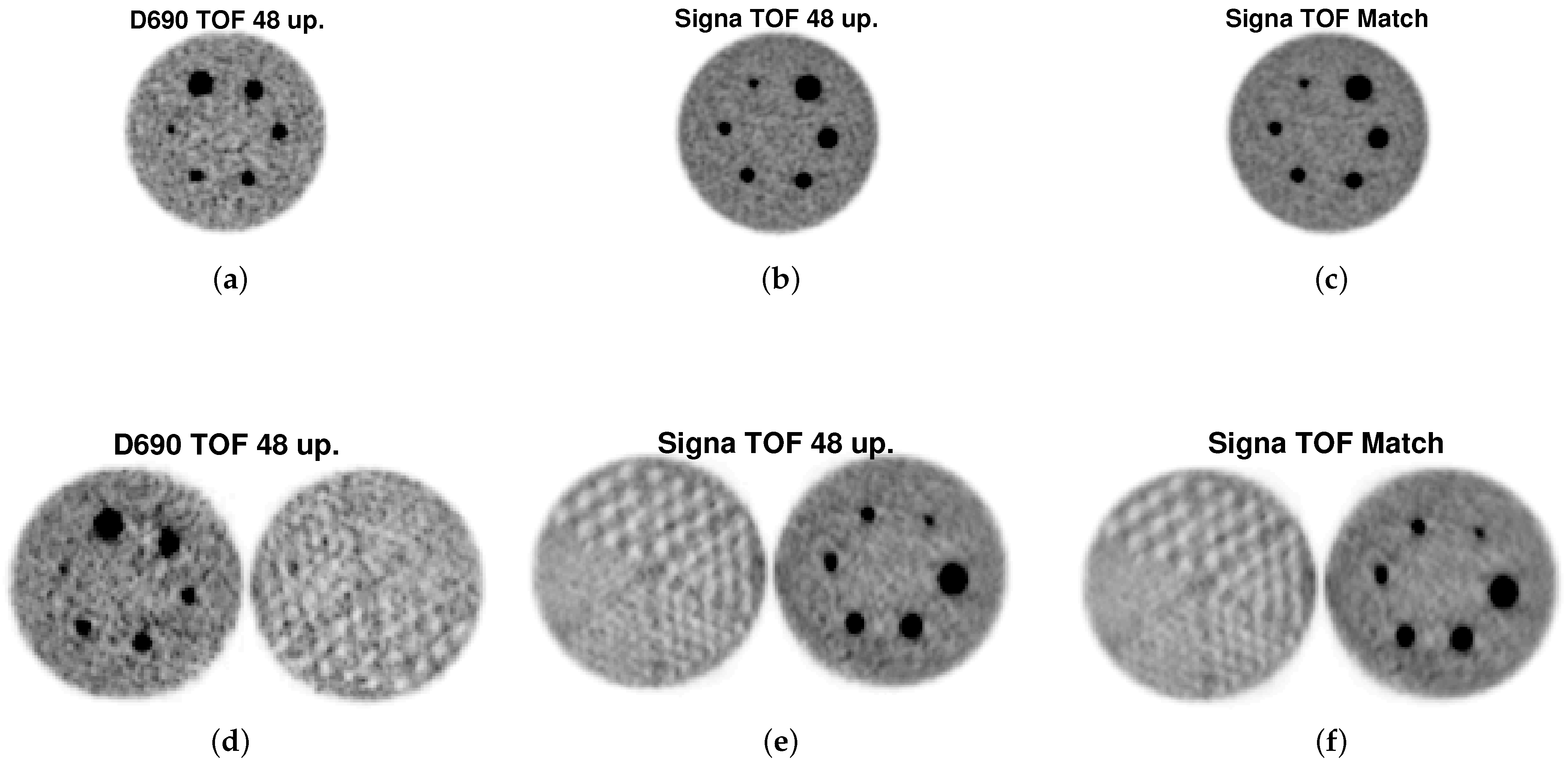
In Figure 4, reconstructions obtained with TOF are shown. The first column contains D690 images at 48 updates, the second SIGNA images at 48 updates, the third SIGNA images at the 32 updates given by the rule to match the D690 48 updates contrast. We can visually appreciate how, at 32 updates, contrast is maintained while noise is reduced.

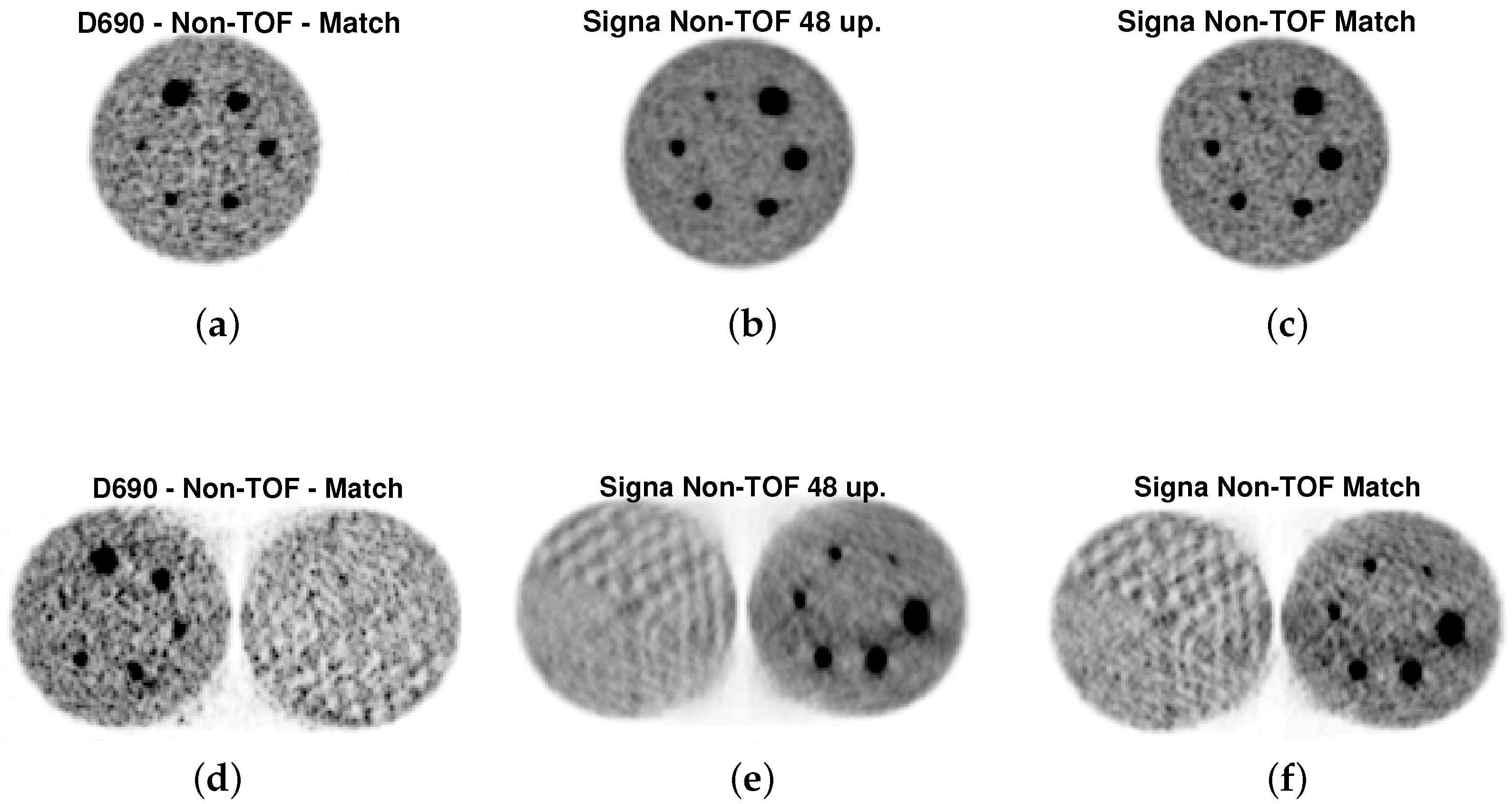
In Figure 5 results for non-TOF reconstructions are shown. Again, in the third column, images at the update number provided by the rule to match the D690 48 update contrast are shown (96 update for the Single configuration, 128 updates for the Double configuration). It is evident, in this case, how the increase in the update number necessary to reach the TOF contrast inevitably leads to a noise augment, particularly in the Double configuration. In this configuration, the smallest sphere is barely visible at 48 updates (Figure 5e); a full recover is associated with a marked noise augment (Figure 5f).

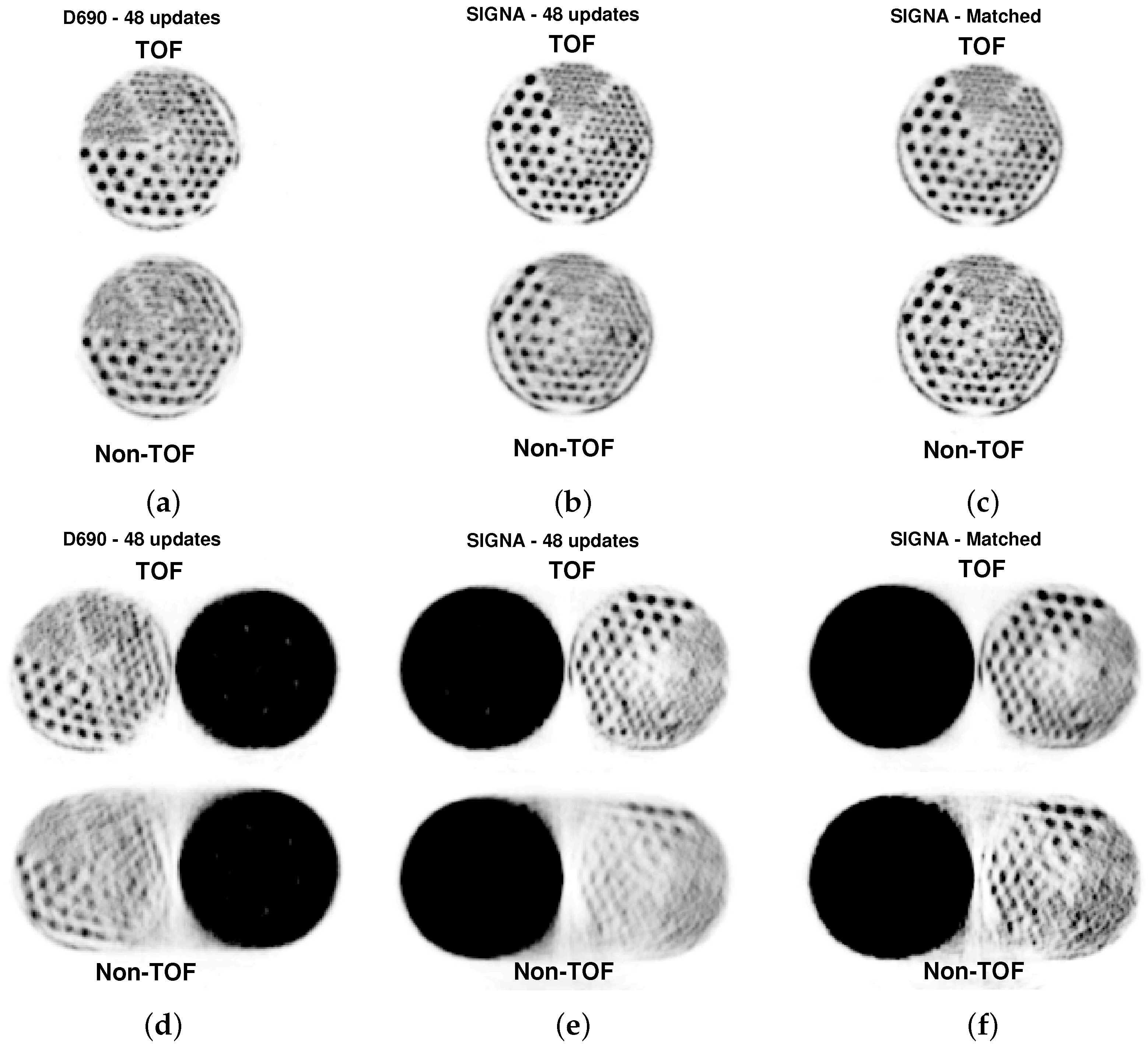
In Figure 6 reconstructions of the hot rods section are shown. The first column contains D690 TOF and non-TOF images at 48 updates, the second SIGNA TOF and non-TOF images at 48 updates, the third Signa TOF and non-TOF images at update numbers given by the rule to match the D690 48 update contrast (32 for TOF, 96 for non-TOF in Single configuration, 128 for non-TOF in Double configuration). We can visually appreciate how, if in the Single configuration hot rods are visible both with TOF and without it, in the Double configuration hot rods visibility strongly depend on their position within the FOV. With TOF, the rule maintains hot rod visibility while reducing noise; in non-TOF it helps recovering hot rods, even if it at increased noise levels.

The results obtained on experimental phantoms are in good agreement with the theoretical predictions. There are only two apparent discrepancies between the theory and experimental data, which can, however, be explained. First, in the non-TOF D690 data at 48 updates, the smallest sphere CR in the Double configuration is comparable instead to lower than the CR in the Single one. This may be due to the sphere position at the border of the phantom and not in the center. The rule derivation shows indeed that the dependence on the background diameter decreases the closer a pixel is to the hot area border.

Secondly, with TOF, on both scanners, CR in the Single configuration is slightly higher than in the Double one. Equation (14) was derived assuming no scatter. In Section 2.2 we found that scatter slows convergence, in a way that it is proportional to its fraction over the total true counts amount. It can be therefore expected that, when increasing object size, the scatter fraction slightly increases, explaining this effect. This was not seen in simulations, where the scatter fraction is held constant.

5. Discussion

It is widely known that TOF accelerates contrast recovery and that the acceleration increases as CTR decreases. However, acceleration concerns also noise; therefore, at the same number of iterations, images reconstructed with TOF are noisier than those reconstructed without TOF [4,13]. For this reason, for a center that installs a new scanner, it might be difficult to set up the OSEM reconstruction protocol that best exploits an improved CTR. Generally, experimental stopping rules are derived on phantoms.

As we showed, however, these are not necessarily applicable to patients, due to the convergence speed dependence on background characteristics. The biggest risk is generally that the high levels of CR measured on phantoms like the NEMA-IQ (which is small) with high contrast ratios (e.g., contrasts as high as 10:1 have been recommended in some guidelines [14]) cannot be replicated in patient studies, especially in large districts with multiple high-activity background structures, like the pelvis or the abdomen.

To find the way to best exploit early stopped OSEM in TOF scanners, we theoretically revised MLEM convergence properties. We found that signal convergence speed increases with signal contrast and dimension. Without TOF, signal convergence decreases with increasing background diameter, i.e., patient dimension. TOF instead, in an ideal setting without random and scatter coincidences, is able to fully eliminate this dependence, thus making early stopped reconstructions robust to variations in patient size and background composition.

An increased fraction of random and scatter coincidences generally decrease the convergence speed. Importantly, TOF significantly reduces random coincidences impact on convergence; the scatter coincidences impact is instead not modified by TOF. As to noise behaviour with iterations, higher frequencies converge more slowly than the lower ones and TOF makes noise convergence faster. At convergence, TOF reduces noise with respect to non-TOF by a factor $\sqrt{D_{eff}/D}$ [1]; however, if a fixed stopping criteria is used, TOF actually increases noise by the inverse of this factor. For this reason, until regularization algorithms become routine in clinical applications, criteria to properly reduce the iteration number while maintaining quantitative accuracy are needed to fully exploit TOF benefits.

In this paper, it was theoretically found that modifying the iteration number by a factor $\Delta t^{\prime }/\Delta t$ matches contrast recovery between two scanners with different CTR. As high frequency noise increases approximately linearly with iterations, this rule achieves, in early stopped reconstructions, the same noise reduction expected at convergence (factor $\sqrt{D_{eff}/D}$). It is widely known from the literature [3,15] that OSEM and MLEM behaviour are slightly different at convergence, since OSEM converges to a limit cycle rather than to a unique solution. This however does not impact on the convergence trend at first iterations, which are the ones concerned by the proposed rule.

The rule has been validated on digital simulations and on real phantoms acquired on two TOF systems with different CTRs. Without TOF, contrast matching on larger background requires to perform more iterations compared to smaller backgrounds and this inevitably inceases noise. With TOF, better CTRs allow reducing the update number, thus maintaining accuracy while minimizing noise.

When deriving the theoretical expression few approximations were required. Most of them require very little assumptions (e.g., $y_i\approx \overline{y_i^{*}}$, or a finite integral for a signal to be recovered). However, to derive an analytical expression we needed to apply the theory to an exemplary simple object, i.e., a large uniform background with a circular signal in its centre, which, at least locally, well represents a typical oncology study. In real conditions of non uniform background convergence will be even faster.

6. Conclusions

A simple early stopping rule for PET TOF systems with different CTRs is able to guarantee contrast matching for the most critical signals while reducing noise. The rule was theoretically derived and successfully validated on digital phantoms and experimental data.

References

- Vunckx, K.; Zhou, L.; Matej, S.; Defrise, M.; Nuyts, J. Fisher Information-Based Evaluation of Image Quality for Time-of-Flight PET. IEEE Trans. Med. Imaging 2010, 29, 311–321. [Google Scholar] [CrossRef] [PubMed]
- Shepp, L.A.; Vardi, Y. Maximum Likelihood Reconstruction for Emission Tomography. IEEE Trans. Med. Imaging 1982, 1, 113–122. [Google Scholar] [CrossRef] [PubMed]
- Hudson, H.M.; Larkin, R.S. Accelerated Image Reconstruction Using Ordered Subsets of Projection Data. IEEE Trans. Med. Imaging 1994, 13, 601–609. [Google Scholar] [CrossRef] [PubMed] [Green Version]
- Bettinardi, V.; Presotto, L.; Rapisarda, E.; Picchio, M.; Gianolli, L.; Gilardi, M.C. Physical Performance of the new hybrid PET/CT Discovery-690. Med. Phys. 2011, 38, 5394–5411. [Google Scholar] [CrossRef] [PubMed]
- Conti, M. Focus on time-of-flight PET: The benefits of improved time resolution. Eur. J. Nucl. Med. Mol. Imaging 2011, 38, 1147–1157. [Google Scholar] [CrossRef] [PubMed]
- Conti, M.; Eriksson, L.; Westerwoudt, V. Estimating Image Quality for Future Generations of TOF PET Scanners. IEEE Trans. Nucl. Sci. 2013, 60, 87–94. [Google Scholar] [CrossRef]
- Karp, J.S.; Surti, S.; Daube-Witherspoon, M.E.; Muehllehner, G. Benefit of Time-of-Flight in PET: Experimental and Clinical Results. J. Nucl. Med. 2008, 49, 462–470. [Google Scholar] [CrossRef] [PubMed] [Green Version]
- van Sluis, J.J.; de Jong, J.; Schaar, J.; Noordzij, W.; van Snick, P.; Dierckx, R.; Borra, R.; Willemsen, A.; Boellaard, R. Performance characteristics of the digital Biograph Vision PET/CT system. J. Nucl. Med. 2019, 60, 1031–1036. [Google Scholar] [CrossRef] [PubMed]
- Nuyts, J. Unconstrained image reconstruction with resolution modelling does not have a unique solution. EJNMMI Phys. 2014, 1, 98. [Google Scholar] [CrossRef] [PubMed] [Green Version]
- Lange, K. Convergence of EM image reconstruction algorithms with Gibbs smoothing. IEEE Trans. Med. Imaging 1990, 9, 439–446. [Google Scholar] [CrossRef] [PubMed]
- Watson, C. Extension of Single Scatter Simulation to Scatter Correction of Time-of-Flight PET. IEEE Trans. Nucl. Sci. 2007, 54, 1679–1686. [Google Scholar] [CrossRef]
- Manjeshwar, R.M.; Ross, S.G.; Iatrou, M.; Deller, T.W.; Stearns, C.W. Fully 3D PET iterative reconstruction using distance-driven projectors and native scanner geometry. IEEE Nucl. Sci. Symp. Conf. Rec. 2007, 5, 2804–2807. [Google Scholar] [CrossRef]
- Conti, M. Why is TOF PET reconstruction a more robust method in the presence of inconsistent data? Phys. Med. Biol. 2011, 56, 155–168. [Google Scholar] [CrossRef] [PubMed]
- Kaalep, A.; Sera, T.; Oyen, W.; Krause, B.J.; Chiti, A.; Liu, Y.; Boellaard, R. EANM/EARL FDG-PET/CT accreditation-summary results from the first 200 accredited imaging systems. Eur. J. Nucl. Med. Mol. Imaging 2018, 45, 412–422. [Google Scholar] [CrossRef] [PubMed] [Green Version]
- Browne, J.; de Pierro, A.B. A row-action alternative to the EM algorithm for maximizing likelihood in emission tomography. IEEE Trans. Med. Imaging 1996, 15, 687–699. [Google Scholar] [CrossRef] [PubMed]
Figure 1.
The exemplar object for which we will perform the calculation. (a) 2D view of the object. Dotted blue line represent a projection direction, passing by the central pixel. (b) Profile of the projection line represented in blue in the left panel.
Figure 2.
True image of the simulated phantom for background diameter mm.
Figure 3.
and background diameter 275 mm. Shaded patches represent ±1 standard error on the mean value. (a) Convergence of circles with contrast , at different distances from the center. (b) Convergence of circles with different activity contrasts.
Figure 4.
TOF Reconstructions of the phantoms in different conditions. Upper: Single acquisitions. Lower: Double acquisition, HCR only for SIGNA shown for clarity. Left (a,d): D690 acquisitions, 48 updates. Center (b,e): SIGNA acquisitions, 48 updates. Right (c,f): SIGNA acquisitions, 32 updates according to the proposed rule.
Figure 5.
Non-TOF Reconstructions of the phantoms in different conditions. Upper: Single acquisitions. Matched non-TOF reconstructions for D690 not shown for clarity Lower: Double acquisition, HCR only for SIGNA shown for clarity. Left (a,d): D690 acquisitions, 48 updates. Center (b,e): SIGNA acquisitions, 48 updates. Right (c,f): SIGNA acquisitions, 32 updates according to the proposed rule.
Figure 6.
Reconstructions of the hot rods section of the phantom in different configurations. Upper rows: Single acquisitions (a–c). Lower rows: double acquisitions (d–f), only HCR shown on Signa for clarity. In each panel the upper row is TOF reconstruction, lower row is non-TOF. Left (a,d): D690, 48 updates. Center (b,e): Signa, 48 Updates. Right (c,f): Proposed stopping rule.