
Chaotic Characteristic Analysis of Vibration Response of Pumping Station Pipeline Using Improved Variational Mode Decomposition Method


 ,
,
Abstract
:1. Introduction
2. Theoretical Aspects
2.1. Identification Method of Chaotic Characteristics
2.1.1. Saturation Correlation Dimension
2.1.2. Largest Lyapunov Exponent
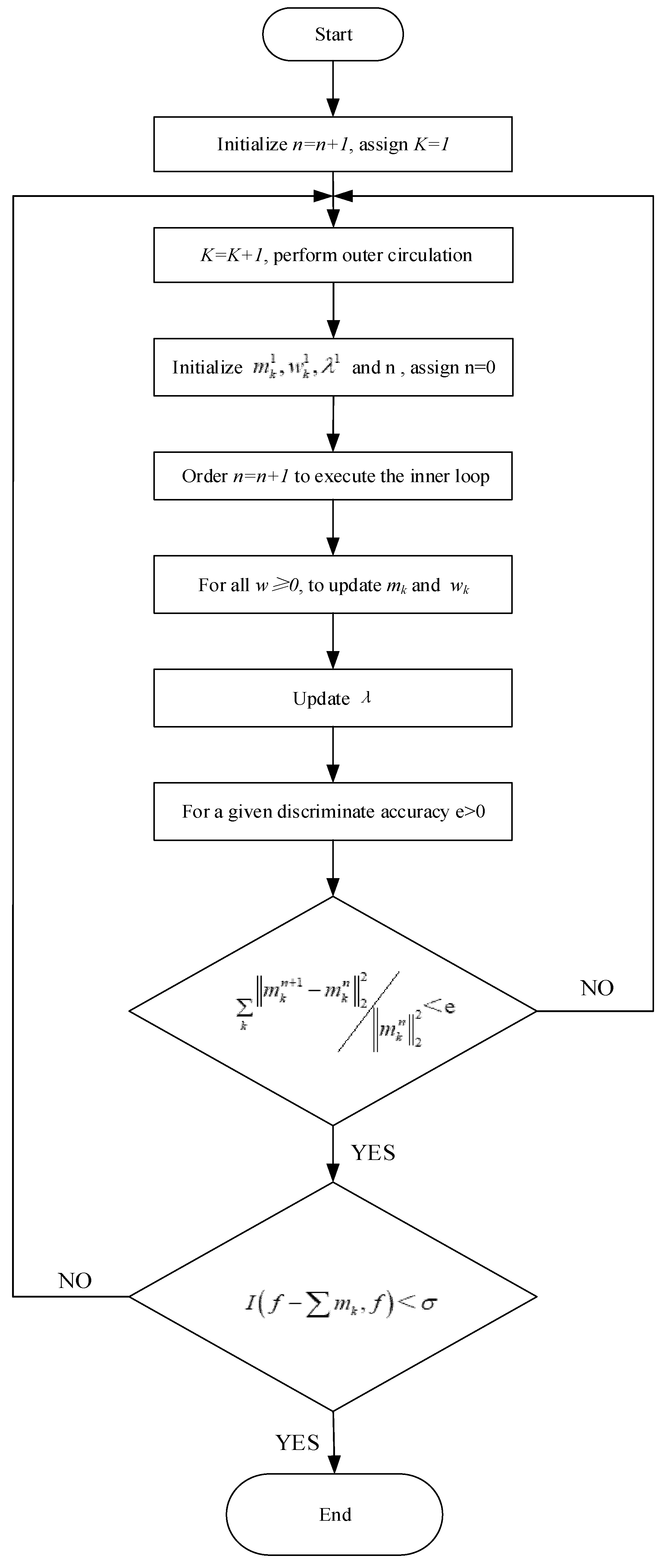
2.2. Improved Variational Mode Decomposition (IVMD)
3. Chaotic Characteristics Analysis of Pipeline Vibration Response
- (1)
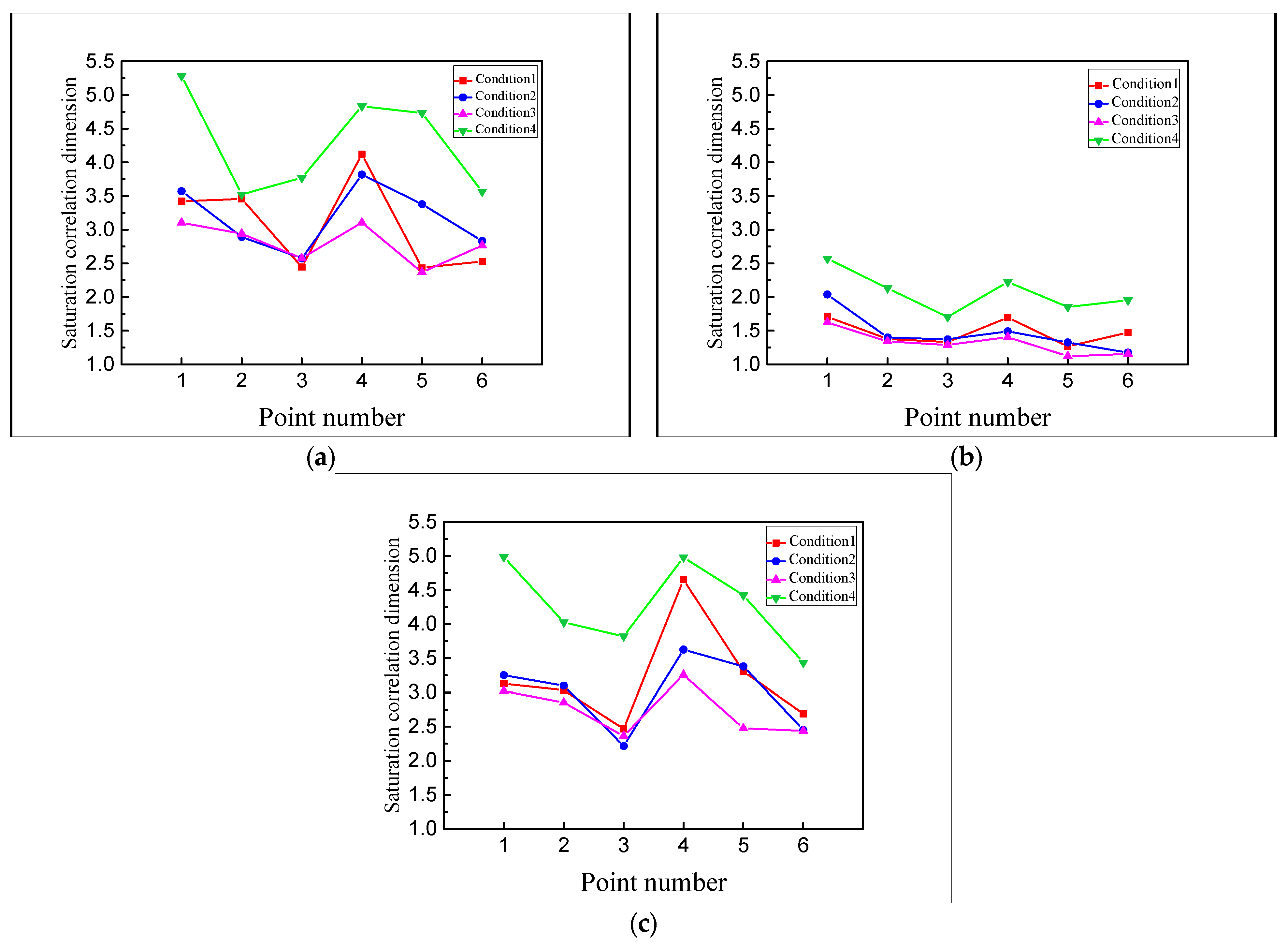
- In general, ranges from 1.156 to 5.283, and they are fractional, indicating that the responses of the pipeline in all directions are chaotic;
- (2)
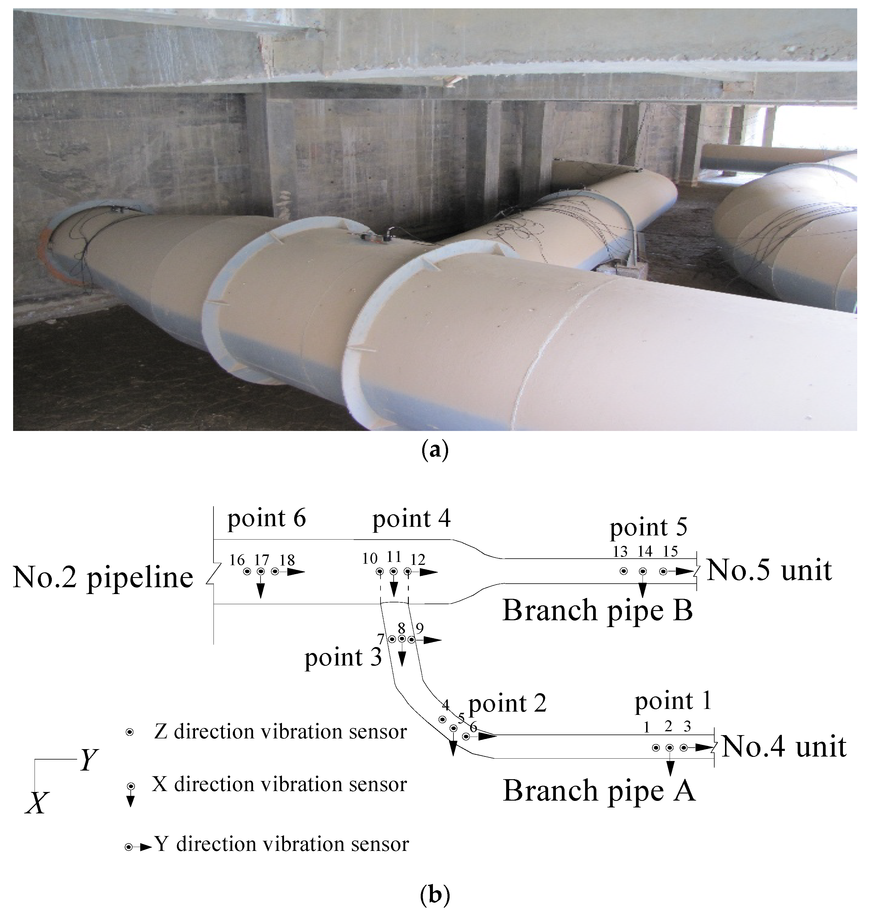
- Compared with the other two directions, the correlation dimension of the axial measurement points (Y-axis) of the main pipe is obviously smaller than that of the other two directions. It shows that the axial vibration of the pipeline has a smaller dimension chaotic attractor and requires fewer independent control variables to describe the dynamic system. This is mainly because the direction of the centrifugal force generated by the centrifugal pump of units is not in the axial direction of the main pipeline;
- (3)
- At the same points, the of each point in condition 4 (No. 4 and 5 units in stable operation) is greater than in other conditions, while the corresponding in condition 3 (No. 4 unit in closing) is less. It indicates that the pipeline vibration is more complicated in the stable conditions of the two units and the complexity of the pipeline vibration is relatively weak in the closed condition. Unit operation increases the uncertainty of the pipeline vibration;
- (4)
- In the same condition, the points near the units (point 1 and 5) and the bifurcated pipe (point 4) reach a relatively larger , indicating that the vibration complexity of the pumping station pipe is greatly affected by the unit’s vibration and the flow pattern stability.
- (1)
- The largest Lyapunov exponents of different points are between 0.0323 and 0.0734, greater than 0. It shows that the measured vibration responses of pipelines have obvious chaotic characteristics. Also, the axial points of the main pipeline (Y-axis) are obviously larger than the other two directions in the same condition, indicating the chaotic characteristics of the points separated from the influence of centrifugal force generated by pumping station units are more obvious;
- (2)
- The of measuring points under condition 4 (No. 4 and 5 units in stable operation) are lower than in other conditions, while the of condition 3 (No. 4 unit closing) is relatively larger. The largest Lyapunov exponent decreases with the start-up of the two units, indicating that the units’ operation weakens the chaotic characteristics of the pipeline vibration;
- (3)
- In the same condition, the of the points near the units (point 1 and 5) are smaller. In contrast, while the of the points at the pipeline’s bifurcation (point 4) are greater than that of other measuring points, indicating that the sudden change of the flow state in the pipeline makes the vibration more chaotic, and the units’ operation reduces the chaotic degree of vibration signals near the units.
4. The Analysis of Multi-Time-Scale Chaotic Characteristics Based on IVMD
- (1)
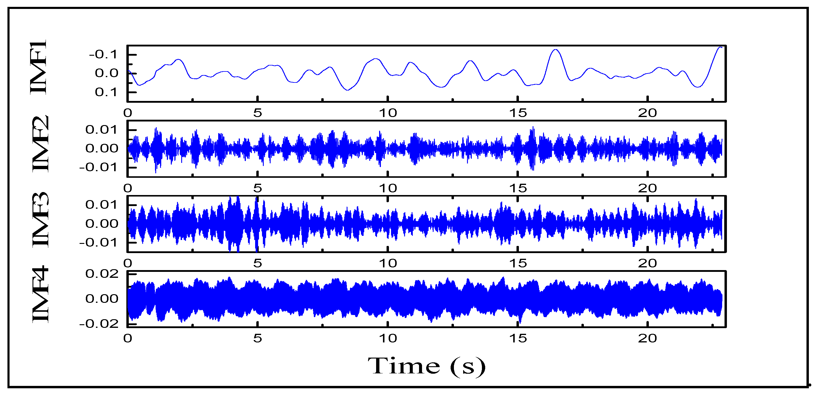
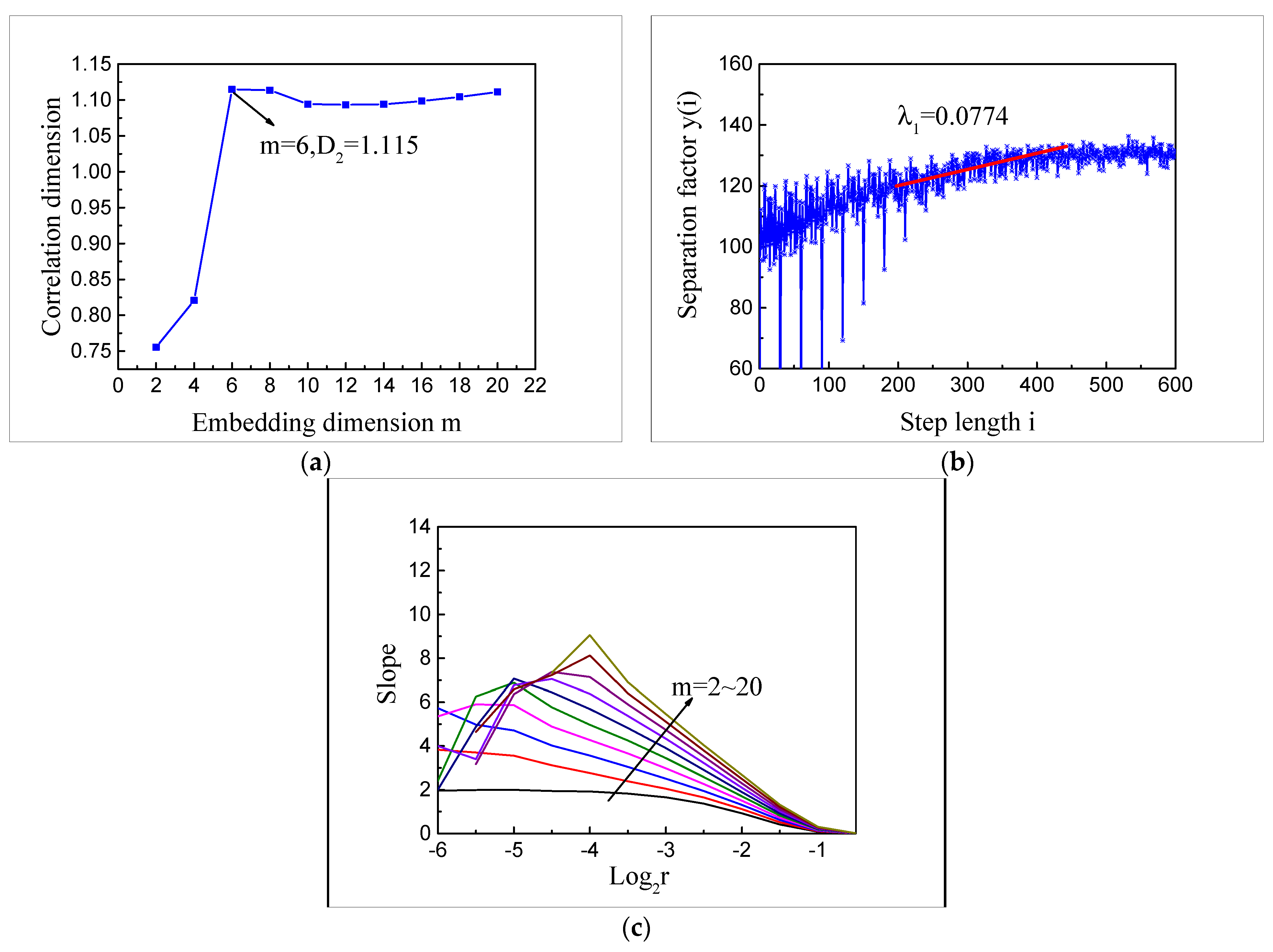
- IMF1, which represents the water pulsation excitation, the saturated correlation dimension 1.115 is a fractal dimension, and the largest Lyapunov exponent is 0.0774 greater than zero, has prominent chaotic characteristics. IMF2 to IMF4, which represent the vibration excitation of the unit’s operation, do not have any chaotic characteristics, indicating that the unit’s operation cannot cause chaotic characteristics of the pumping station pipeline vibration;
- (2)
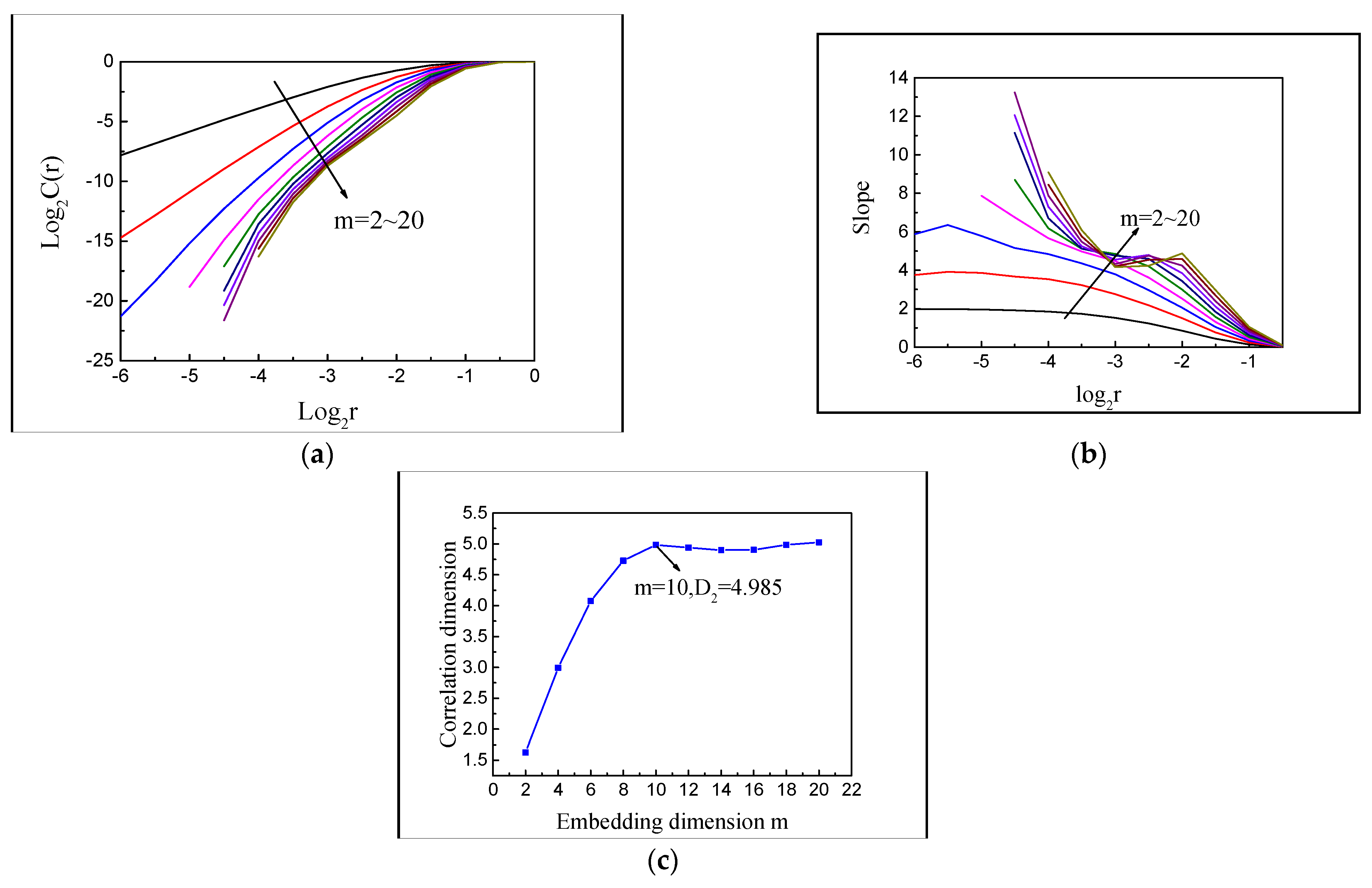
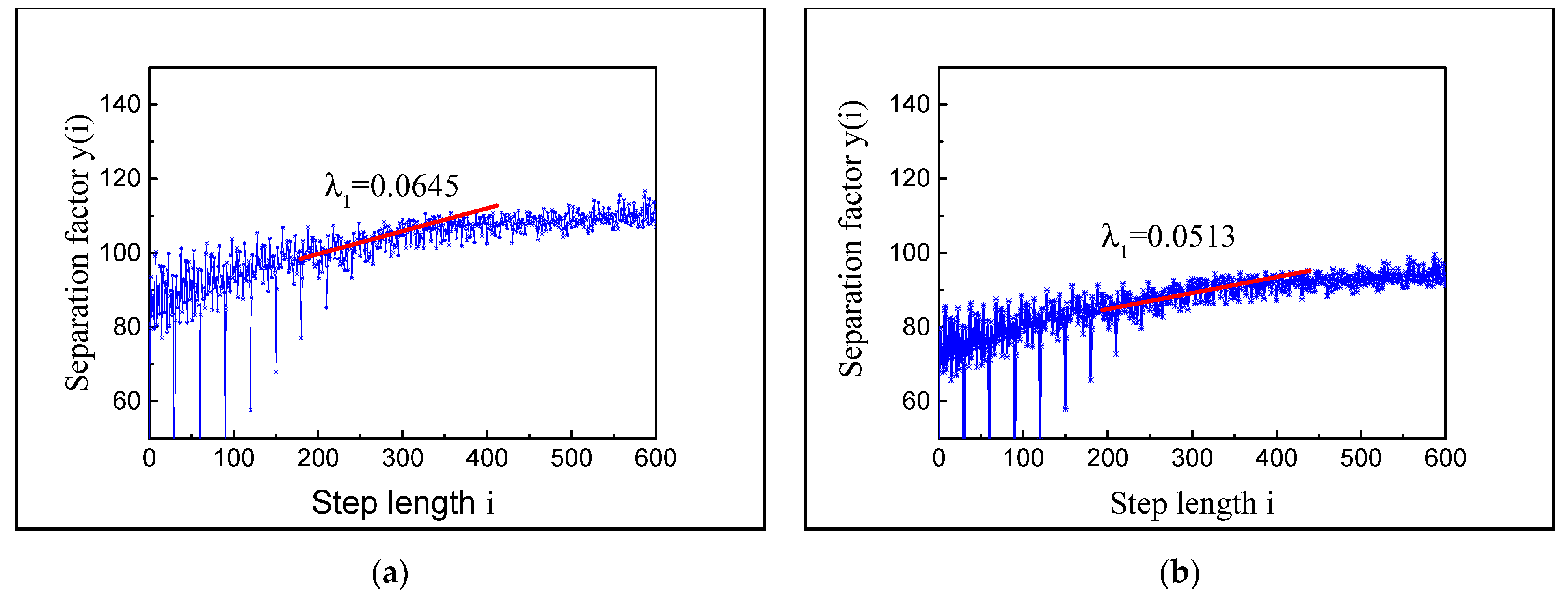
- After eliminating the IMFs (IMF2 to IMF4) caused by the unit’s operation with no chaotic characteristics, the saturation correlation dimension of the pipeline vibration response decreases from 4.985 to 1.115. At the same time the largest Lyapunov exponent increases from 0.0513 to 0.0774, that is, the complexity of the pipeline vibration decreases, and its chaotic characteristics are more evident. This shows that when the pumping station pipeline vibrates, the water pulsation excitation makes its vibration have obvious chaotic characteristics. In contrast, vibration excitation generated by the unit’s operation masks the chaotic characteristics of the pumping station pipeline and increases the uncertainty of the pipeline vibration.
5. Conclusions
- (1)
- Comparing the saturation correlation dimension D2 among the vibration responses of the pumping station pipeline under different conditions, the D2 of the measuring points are distributed in the range of 1.156–5.283, and all are fractions, which show that the vibration of the pumping station pipeline has chaotic characteristics. The axial vibration of the pipeline presents a chaotic attractor with a lower dimension (1.156~2.569), and the vibration form is relatively simple. At the same time, the D2 of conditions and points which are greatly affected by the unit’s operation have a larger value (3.021~5.283), and the vibration form is more complex;
- (2)
- The Lyapunov exponents λ1 of measuring points under different conditions are between 0.0513 and 0.0774. With the opening of two units, the largest Lyapunov exponent λ1 decreases accordingly, suggesting that the unit’s operation weakens the chaotic characteristics of the pipeline vibration. The λ1 of points at the bifurcation are larger than those of other points under the same condition. The chaotic characteristics of the vibration at the bifurcation are enhanced by the sudden expansion of the pipe diameter at the bifurcation and the impact of water heads at different flow velocities;
- (3)
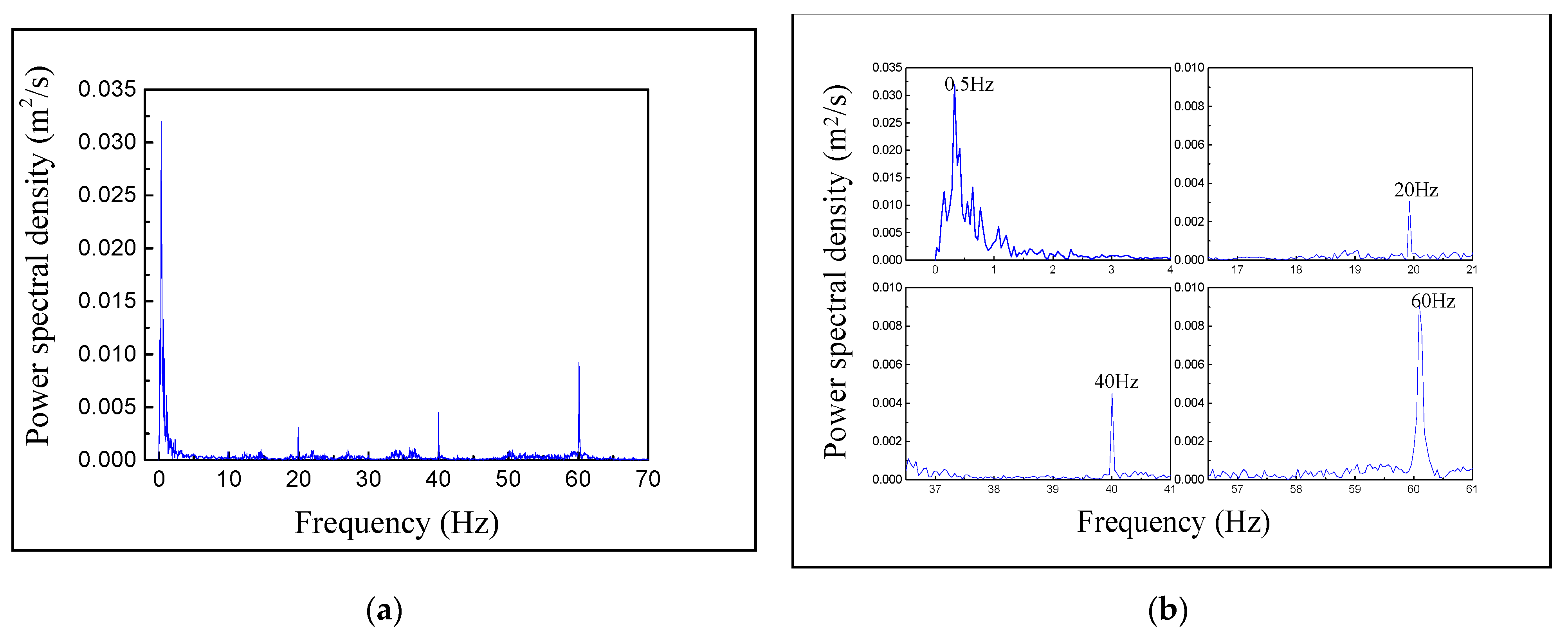
- After the IVMD decomposition of the vibration response of specific points under the unit’s operation conditions, the chaotic characteristics of the IMFs are analysed. The results show that the saturation correlation dimension D2 of IMF1 representing water pulsation excitation in the pipeline is 1.115, and the largest Lyapunov exponent is 0.0774. The IMF2 to IMF4 representing the blade frequency, the rotation frequency, and the frequency doubling vibration excitation generated by the unit’s operation do not have chaotic characteristics. It indicates that the chaotic character of the pumping station pipeline is mainly caused by water pulsation in the pipeline, and the vibration caused by the unit masks the chaotic characteristic of the pipeline, which makes the pipeline vibration system more complex.
Author Contributions
Funding
Institutional Review Board Statement
Informed Consent Statement
Data Availability Statement
Conflicts of Interest
Abbreviations
| IVMD | improved variational mode decomposition |
| IMF | intrinsic mode function |
References
- Jain, S.V.; Patel, R.N. Investigations on pump running in turbine mode: A review of the state-of-the-art. Renew. Sustain. Energy Rev. 2014, 30, 841–868. [Google Scholar] [CrossRef]
- Lu, H.; Huang, K.; Wu, S. Vibration and Stress Analyses of Positive Displacement Pump Pipeline Systems in Oil Transportation Stations. J. Pipeline Syst. Eng. Pract. 2016, 7, 05015002. [Google Scholar] [CrossRef]
- Pergushev, L.P.; Fattakhov, R.B.; Sakhabutdinov, R.Z. Analysis of operation of booster pumping station. Neftyanoe Khozyaistvo 2005, 5, 134–137. [Google Scholar]
- Jiang, Q. Research on Coupled Vibration Characteristics and Vibration Control of Pipeline of Cascade Pumping Station. Master’s Thesis, North China University of Water Resources and Electric Power, Zhengzhou, China, 2017. [Google Scholar]
- PaïDoussis, M.P.; Li, G.X. Pipes Conveying Fluid: A Model Dynamical Problem. J. Fluids Struct. 1993, 7, 137–204. [Google Scholar] [CrossRef]
- Tang, D.M.; Dowell, E.H. Chaotic oscillations of a cantilevered pipe conveying fluid. J. Fluids Struct. 1988, 2, 263–283. [Google Scholar] [CrossRef]
- Sinir, B.G. Bifurcation and chaos of slightly curved pipes. Math. Comput. Appl. 2007, 15, 490–502. [Google Scholar] [CrossRef]
- Zhao, D.; Liu, J.; Wu, C.Q. Stability and local bifurcation of parameter-excited vibration of pipes conveying pulsating fluid under thermal loading. Appl. Math. Mech. 2015, 36, 1017–1032. [Google Scholar] [CrossRef]
- Liu, S.T.; Sun, F.Y.; Shen, S.L. Chaos Behaviour of Molecular Orbit. Chin. Phys. Lett. 2007, 24, 3590. [Google Scholar]
- Hiruta, K.; Fujita, A.; Inagaki, K. 28a-B-13 Fractal Structure on Poincare Surface of Section of Chaotic Attractor. Phys. Soc. Jpn. JPS 1994. [Google Scholar]
- Yang, L.; Shan, C.L. Dual Chaos SVPWM Technology and its Power Spectral Density Analysis. East China Electr. Power 2013, 41, 0579–0583. [Google Scholar]
- Liu, Y.; Wen, B.; Yang, J. Chaos and Fractal Dimension Research of Investment Time Series. J. Northeast. Univ. Nat. Sci. 2001, 22, 524–526. [Google Scholar]
- Jayaraman, A.; Scheel, J.D.; Greenside, H.S. Characterization of the domain chaos convection state by the largest Lyapunov exponent. Phys. Rev. E 2006, 74 Pt 1, 016209. [Google Scholar] [CrossRef] [PubMed] [Green Version]
- Rosenstein, M.T.; Collins, J.J.; Luca, C.J.D. A practical method for calculating largest Lyapunov exponents from small data sets. Phys. D Nonlinear Phenom. 1993, 65, 117–134. [Google Scholar] [CrossRef]
- Dragomiretskiy, K.; Zosso, D. Variational mode decomposition. Trans. Signal Process. 2014, 62, 531–544. [Google Scholar] [CrossRef]
- Zhang, N.; Zhu, Y.L.; Gao, Y.F. An On-Line Detection Method of Transformer Winding Deformation Based on Variational Mode Decomposition and Probability Density Estimation. Power Syst. Technol. 2016, 40, 297–302. [Google Scholar]
- Liu, C.L.; Yan, X. Fault diagnosis of a wind turbine rolling bearing based on variational mode decomposition and condition identification. J. Chin. Soc. Power Eng. 2017, 37, 273–278. [Google Scholar]
- Hestenes, M.R. Multiplier and gradient methods. J. Optim. Theory Appl. 1969, 4, 303–320. [Google Scholar] [CrossRef]
- Tang, G.J.; Wang, X.L. Parameter optimized variational mode decomposition method with application to incipient fault diagnosis of rolling bearing. J. Xi’an Jiaotong Univ. 2015, 49, 73–81. [Google Scholar]
- Hu, A.J. Research on the Application of Hilbert-Huang Transform in Vibration Signal Analysis of Rotating Machinery. Master’s Thesis, North China Electric Power University, Baoding, China, 2008. [Google Scholar]
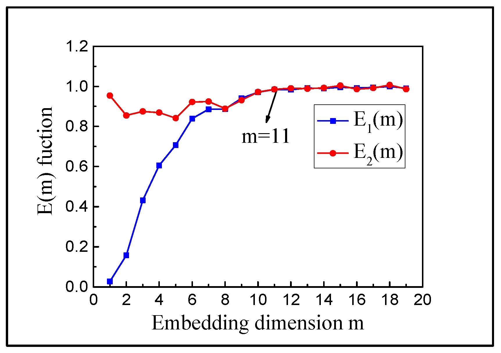
- Cao, L.Y. Practical method for determining the minimum embedding dimension of a scalar time series. Phys. D Nonlinear Phenom. 1997, 110, 43–50. [Google Scholar] [CrossRef]
- Grassberger, P.; Procaccia, I. Measuring Strangeness Strange Attractors. Phys. D Nonlinear Phenom. 1983, 9, 189–208. [Google Scholar] [CrossRef]
- Zhang, J.W.; Jiang, Q.; Wang, T. Analysis of vibration characteristics of pipeline of trapezoid pumping station based on prototype observation. Trans. Chin. Soc. Agric. Eng. 2017, 33, 77–83. [Google Scholar]
- Zhang, J.W.; Li, Z.Y.; Yan, P.; Li, Y.; Huang, J.L. The Method for Determining Optimal Analysis Length of Vibration Data Based on Improved Multiscale Permutation Entropy. Shock Vib. 2021, 2021, 6654089. [Google Scholar]
- Lv, J.H.; Lu, J.A. Chaotic Time Series Analysis and Its Application; Wuhan University Press: Wuhan, China, 2002. [Google Scholar]
- Wang, Z.; Zheng, L.; Junyuan, W. Application of a New Enhanced Deconvolution Method in Gearbox Fault Diagnosis. Appl. Sci. 2019, 9, 5313. [Google Scholar] [CrossRef] [Green Version]


| Cases | Description of Working Conditions | Sampling Time/s | Sampling Frequency/Hz |
|---|---|---|---|
| 1 | No. 4 unit stable operating | 900 | 512 |
| 2 | No. 4 unit opening | 1800 | 512 |
| 3 | No. 4 unit closing | 1800 | 512 |
| 4 | No. 4 and 5 units stable operating | 900 | 180 |
Publisher’s Note: MDPI stays neutral with regard to jurisdictional claims in published maps and institutional affiliations. |
© 2021 by the authors. Licensee MDPI, Basel, Switzerland. This article is an open access article distributed under the terms and conditions of the Creative Commons Attribution (CC BY) license (https://creativecommons.org/licenses/by/4.0/).
Share and Cite
Jiang, L.; Ma, Z.; Zhang, J.; Khan, M.Y.A.; Cheng, M.; Wang, L. Chaotic Characteristic Analysis of Vibration Response of Pumping Station Pipeline Using Improved Variational Mode Decomposition Method. Appl. Sci. 2021, 11, 8864. https://0-doi-org.brum.beds.ac.uk/10.3390/app11198864
Jiang L, Ma Z, Zhang J, Khan MYA, Cheng M, Wang L. Chaotic Characteristic Analysis of Vibration Response of Pumping Station Pipeline Using Improved Variational Mode Decomposition Method. Applied Sciences. 2021; 11(19):8864. https://0-doi-org.brum.beds.ac.uk/10.3390/app11198864
Chicago/Turabian StyleJiang, Li, Zhenyue Ma, Jianwei Zhang, Mohd Yawar Ali Khan, Mengran Cheng, and Libin Wang. 2021. "Chaotic Characteristic Analysis of Vibration Response of Pumping Station Pipeline Using Improved Variational Mode Decomposition Method" Applied Sciences 11, no. 19: 8864. https://0-doi-org.brum.beds.ac.uk/10.3390/app11198864