Development of an Analytical Model to Determine the Heat Fluxes to a Structural Element Due to a Travelling Fire

Abstract

The term “travelling fire” is used to label fires which burn locally and move across the floor over a period of time in large compartments. Through experimental and numerical campaigns and while observing the tragic travelling fire events, it became clear that such fires imply a transient heating of the surrounding structure. The necessity to better characterize the thermal impact generated on the structure by a travelling fire motivated the development of an analytical model allowing to capture, in a simple manner, the multidimensional transient heating of a structure considering the effect of the ventilation. This paper first presents the basic assumptions of a new analytical model which is based on the virtual solid flame concept; a comparison of the steel temperatures measured during a travelling fire test in a steel-framed building with the ones obtained analytically is then presented. The limitations inherent to the analyticity of the model are also discussed. This paper suggests that the developed analytical model can allow for both an acceptable representation of the travelling fire in terms of fire spread and steel temperatures while not being computationally demanding, making it potentially desirable for pre-design.

1. Introduction

Several developments were recently made to represent in a detailed manner the thermal effect of a travelling fire through CFD (computational fluid dynamics) numerical analyses (Horova [1], Degler et al. [2], Charlier et al. [3,4], Dai et al. [5]), providing a great deal of relevant information in terms of fire dynamics that can be used as input for subsequent structural analyses. Although progress in numerical modelling is crucial, it is equally important to expand and advance the analytical models for structural design and pre-design purposes. Indeed, analytical methods are complementary to more complex and less accessible numerical ones. They provide scientific and reliable routes commonly used by practitioners to quickly and easily develop schemes, understand the relationships between parameters and provide a means to independently check numerical solutions. These methods can sometimes present limitations inherent to their simplicity but their results can, where there is necessity in doing so, be improved numerically at a later stage. As for numerical models, it is important to improve analytical ones too, to also allow them to match the complexity of the considered problem.

During the last decade, analytical models were developed and generated the first frameworks allowing the characterisation of fires for building typologies where a generalised fire does not develop. In 2012, SternGottfried and Rein [6] proposed a methodology for modelling travelling fires in large compartments contrasting the methods that assume uniform burning. The model was later on improved by Rackauskaite et al. [7] by notably reducing the range of possible fire sizes. This model considers that the fire-induced thermal field is divided in two regions: the near field and the far field. The ventilation conditions are not accounted for in this methodology and the near field temperature applies along the full height of the compartment. In 2015, Horová [1] developed a simple method to determine the thermal action of a spreading fire for the design of structures: this model is based on the idea of repetitious heat release rate parametric curves acting with required time offset in neighbouring parts of a structure. In 2016, Vassart et al. [8] developed models for localised fires to predict the radiative heat flux to a structural element (the analytical model being detailed by Tondini et al. [9]). This methodology allows evaluating the heat fluxes in three dimensions and a transient heating of a structural element. However, in this model, localised fires are assumed to remain in given locations and do not reflect the possible travelling nature of the fire. In 2020, Dai et al. [10] proposed a new travelling fire framework (“ETFM”) considering a mobile version of Hasemi model—a localised fire model—and a smoke layer computed by the “FIRM” zone model [11]. A limitation of the ETFM framework is the limited applicability of Hasemi’s localised fire model which is applicable only if the fire impacts the ceiling. The above mentioned limitations motivated the development of a new analytical model allowing to determine the heat fluxes capturing the transient heating of a structure, both along the direction followed by the fire and along the height of the enclosure whilst taking into account the influence of the ventilation boundary conditions. The present paper describes this development.

First, this paper presents the basic assumptions of the analytical model. The fire representation is based on the virtual solid flame concept developed in the frame of the “LOCAFI” project [8,9]. The fire is represented as a rectangular volume with a basis given by the burning bands which evolve as a function of time. Contrarily to the LOCAFI model where the virtual solid flame has a conical shape, it is here considered as (a succession of) parallelepiped rectangles. The model uses, amongst other parameters, the view factors which measure the fraction of the total radiative heat leaving a given radiating surface that arrives at a given receiving surface, implying a multi-dimensional consideration. The model relies on several successive steps: the evaluation of the fire geometry and its position in the compartment, the evaluation of the flame temperature, the evaluation of the heat fluxes in the compartment, and finally, the evaluation of the temperature of a steel structural member located in the compartment. To evaluate the heat fluxes, different zones are defined depending on the location of the target and on whether the flame impacts or not the ceiling. In addition, the transient evaluation of steel temperatures of a structural member placed in the compartment is computed following an iterative procedure from Eurocode 3.

The effect of the ventilation is considered through a simple concept: the burning rate (kW/m²) in the compartment may be (momentarily) modified during the course of the fire when the fire is air controlled. The latter situation is evaluated following an approach initially proposed by Kawagoe [12] which considers that the fire power is limited by the oxygen which can enter in the compartment through the openings, using the opening factor to assess the ventilation limitation.

Then, this paper presents a comparison of the temperatures measured during a travelling fire test in a column made of a hot-rolled steel profile with the ones obtained through the analytical model: the similitudes and differences are discussed. This paper suggests that the developed analytical model can allow for an acceptable representation of the travelling fire in terms of fire spread and of steel temperatures, despite limitations inherent to the analyticity of the model, making it potentially usable for the pre-design stage of a building structure.

2. Development of a New Analytical Model Based on the Virtual Solid Flame Concept

2.1. Basic Assumptions

The development of an analytical procedure requires the simplification of both the compartment and the fire representation. The following assumptions were therefore considered:

• The plan view of the compartment has a rectangular shape;
• The floor and the ceiling of the compartment are flat and horizontal;
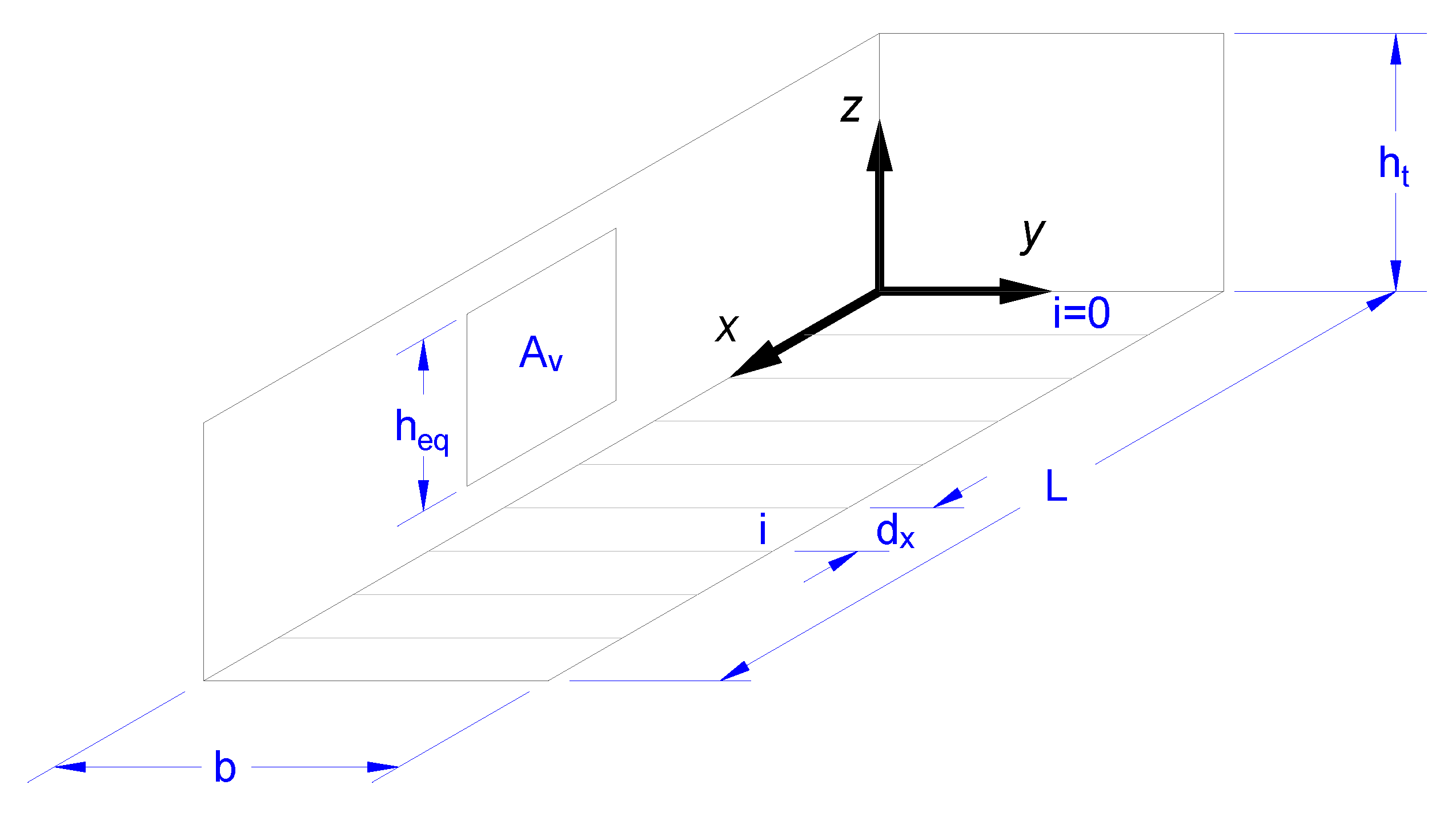
• The plan view is divided into bands of equal width parallel to the defined plan dimension b (see Figure 1);
• The fire load is uniformly distributed in the compartment, covering the whole floor area;
• The fire starts in the band close to one of the façades and spreads from band to band;
• The fire is represented as a rectangular volume the basis of which is given by the burning bands;
• The spread rate is given as an input and remains constant during the duration of the fire;
• The rate of heat release in all burning bands is reduced if the fire is ventilation controlled;
• The openings defined in the method are considered as fully open.

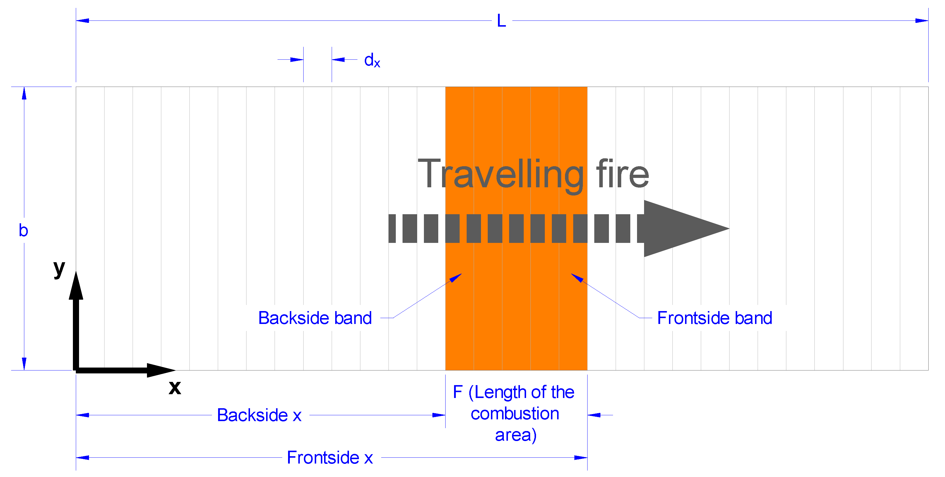
2.2. Evaluation of the Fire Geometry and Its Position in the Compartment

The following symbols are used (referring to Figure 1):

• d_x = width of each band;
• n_dx = quantity of bands;
• The index i is used to denote the band number. Band (1) extends from x = 0 to x = d_x, band (i) extends from x = (i − 1).d_x to x = i.d_x, etc.;
• At time t = 0, fire starts in band (1) only and will thus spread towards increasing values of x, i.e., to band (2), and then band (3), etc.
• The following inputs have to be given to describe the problem:
• Width b, length L, and floor to ceiling distance h_t of the compartment [m];
• Width of the bands d_x [m], the total number of bands nd_x is therefore evaluated by rounding up the ratio L/d_x, and d_x is then re-evaluated as d_x = L/nd_x;
• The design value of the fire load density q_f,d [MJ/m²];
• The rate of heat release density RHR_f [kW/m²];
• The height of the fire load basis h_base (to allow for elevated combustible, the floor height being situated at 0 m height) [m];
• The fire spread rate v [mm/s];
• The combustion factor m (fixed to 0.8 in EN1991-1-2 [13]) [-];
• The effective heat of combustion of the fire load H [MJ/kg];
• The total area of vertical openings A_v (as the openings are considered as fully open, this area should correspond to the area of broken or open windows and doors) [m²];
• The equivalent height of the openings h_eq [m];
• The time-step dt [s].

The ratio q_f,d/RHR_f corresponds to the time required to consume all the fire load present within a band, and the ratio d_x/v corresponds to the time needed for the combustion front to cross a band. The band width d_x should be defined to be lower than the ratio (ν . q_f,d/RHR_f), otherwise the fire will extinguish in one band before spreading to the adjacent one. The procedure considers the dimensions of the vertical openings (thus the amount of oxygen present to sustain combustion) but not their locations within the compartment. This implies that any local effect resulting from fire passing from a ventilated zone to an under-ventilated zone—and vice versa—(implying, amongst other, acceleration or deceleration of the fire) is disregarded. The parameter h_base allows the consideration of situations in which the fire load does not lay on the floor (i.e., at z = 0), but at a given height above the floor (i.e., at z = h_base).

2.2.1. Position of the Fire

The position of the fire at a certain time in the compartment is deduced from the burning bands: the state of each band during the fire is either burning or not burning depending whether combustion is taking place or not at this moment in this band. This state is characterised by a binary variable burning that has the value of 1 (burning) or 0 (non-burning, i.e., not yet burnt or burnt out). The propagation is driven by the fire spread rate. When a band i has an adjacent band i-1 that has been burning for a duration t_prop = d_x/ν, the value of burning (i) is set to 1. Within a band, when the fire load density drops down to 0, burning in this cell becomes 0. The combustion area is delimited by the frontside and backside of the burning bands.

2.2.2. Power and Fire Load Density

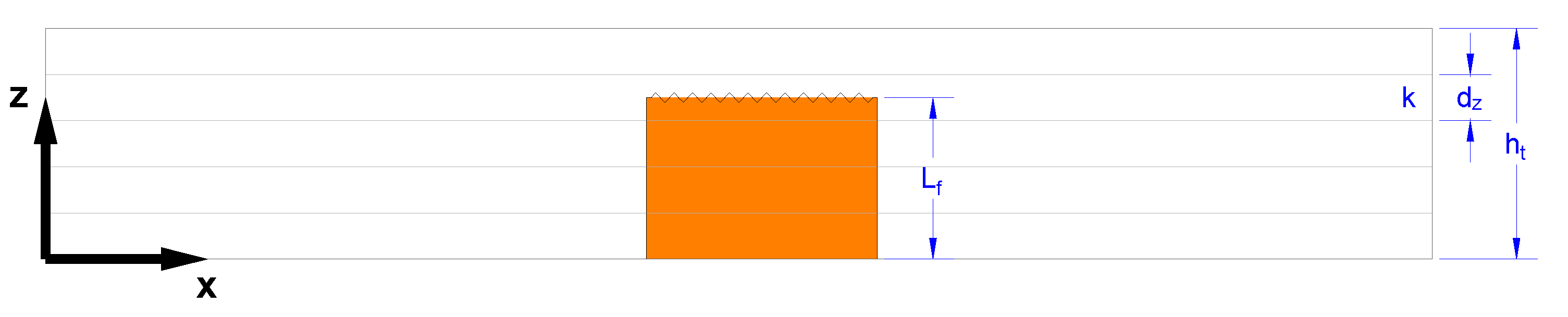
The rate of heat release density RHR_f, given as input, is a constant. The parameter R is here introduced as the variable value of the rate of heat release density (kW/m²) which can vary at each time-step: it may change during the course of the fire depending on the ventilation conditions. The initial value of R is RHR_f, and the following simple assumption is considered: R is (momentarily) decreased when the fire is air controlled, and such situation is evaluated through Equation (3) from EN 1991-1-2 Annex E [13]. This equation considers that the power is limited by the oxygen which can enter the compartment through the openings, using the size of the openings to consider the ventilation limitation. The first use of this parameter is attributed to Kawagoe [12]. The empirical observation was made that wood fires in rooms with small windows appeared to burn at a rate approximately stoichiometric [14]. The present methodology disregards the influence of the environment on the fire plume (such as the boundary conditions, for example the effect of isolated openings), as well as other complex phenomena’s (combustion efficiency, evolution of the temperature, chemical reaction kinetics (Merci and Beji [15])). These considerations lead to the procedure described below.

The total power Q (MW), released by the fire in the compartment, is evaluated through the following equation (A_band being the area of one burning band, i.e., d_x multiplied by b):

$$Q=\left(R/1000\right).A_{band}{\displaystyle \sum }_{i=1}^{n}burning\left(i\right)$$

(1)

The limit value Q_lim given by the following equation (EN1991-1-2 [13]):

Q_lim = (1/10) . m . H . A_v . h_eq^0.5

(2)

If Q ≤ Q_lim then R = RHR_f.

If Q > Q_lim then R is adapted to reach Q = Q_lim, namely:

$$R=\frac{Q_{lim}}{{{\displaystyle \sum }}_{i=1}^n{A}_{band} . burning\left(i\right)}$$

(3)

The fire load density q in a band depends on the band i and on time. The initial value is set to q_f,d in each band, and this value can decrease during the course of the fire. In each band i, the variation of the fire load density as a function of time depends on the value of the variable burning and on the value of R:

$$\frac{dq\left(i\right)}{dt}=0\mathrm{if}\mathit{burning}(i)=0$$

(4)

$$\frac{dq\left(i\right)}{dt}=-R\mathrm{if}\mathit{burning}(i)=1$$

(5)

2.2.3. Flame Length

The flame length is evaluated based on the localised fire theory, and more precisely on the model developed by Heskestad [16,17]. This model allows evaluating the mean flame height of a turbulent diffusion flame in buoyancy regime and was validated against experimental data in the frame of the research conducted by Zukoski et al. [14]. The flame length actually refers to the mean luminous flame height L_f, which is the distance between the fire source and the point where the intermittency has decreased by half. The Heskestad correlation [17] is given in Equation (6), considering the heat of combustion of the fuel as 3 kJ/g (air) (value approximately constant for most of the fuels [18]) and normal atmospheric conditions (T∞ = 20 °C and p = 101325 Pa), with L_f being the flame length (m), D the diameter of the flame source (m) and Q_loc the rate of heat release of the localised fire (kW). An analogous correlation (Equation (7)) is given in EN 1991-1-2 [13] where Q_loc is now expressed in (W), and this correlation was considered in the present analytical model.

$$L_f=-1.02 D+0.23 Q_{loc}{}^{2/5}$$

(6)

$$L_f=-1.02 D+0.0148 Q_{loc}{}^{2/5}$$

(7)

It has to be noted that the correlation linking the flame length with the diameter of the flame source and the rate of heat release is valid if the surrounding air is uncontaminated by fire products and is uniform in temperature. Such conditions are not met in travelling fire scenario, nevertheless the predictions given by the Heskestad correlation are in good agreement with the experimental results (as shown in this paper), even though this empirical equations was not precisely conceived for that purpose.

To apply Heskestad correlation, a diameter D of the fire basis needs to be defined. It is here taken as the minimum of b (width of the compartment and therefore width of the combustion area) and the length of the combustion area F (see Figure 2).

The flame height H_f is then computed based on Equation (7), simply adding the height of the fire load basis h_base to allow the consideration of a fire load which does not lay on the floor (see Equation (8)). The power released by the fictitious localised fire Q_loc inscribed in the circular combustion area is computed following Equation (9). The equation for L_f (and H_f) may lead to negative values, as well as values greater than the floor to ceiling distance ht. In such cases, L_f is bounded to 0 and h_t, respectively.

$$H_f=L_f+h_{base}=-1.02 D+0.0148 Q_{loc}{}^{\frac{2}{5}}+h_{base}$$

(8)

$$Q_{loc}=R\times \pi \frac{D^2}{4}$$

(9)

These correlations detailed above were derived for the following range of application: the diameter of the fire is limited by D ≤ 10 m and the rate of heat release of the fire by Q ≤ 50 MW, but these limitations were disregarded, in the lack of more precise equations. It is nevertheless worth to point out that the virtual solid flame model (project LOCAFI [8]) was compared against experimental data of kerosene pool fires as large as 50 m and characterised by RHR in the order of 3000 MW (Randaxhe [19]). McCaffrey [20] has reviewed effects on flame height of placing fire sources next to a wall or in a corner but these effects were reported to be small, and no such consideration is made in the present analytical procedure. Also, windblown flames (i.e., bent or deflected flames) were not considered.

2.3. Evaluation of the Flame Temperature and of the Heat Fluxes in the Compartment

2.3.1. Flame Temperature

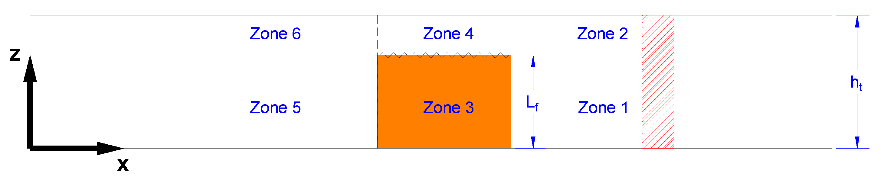
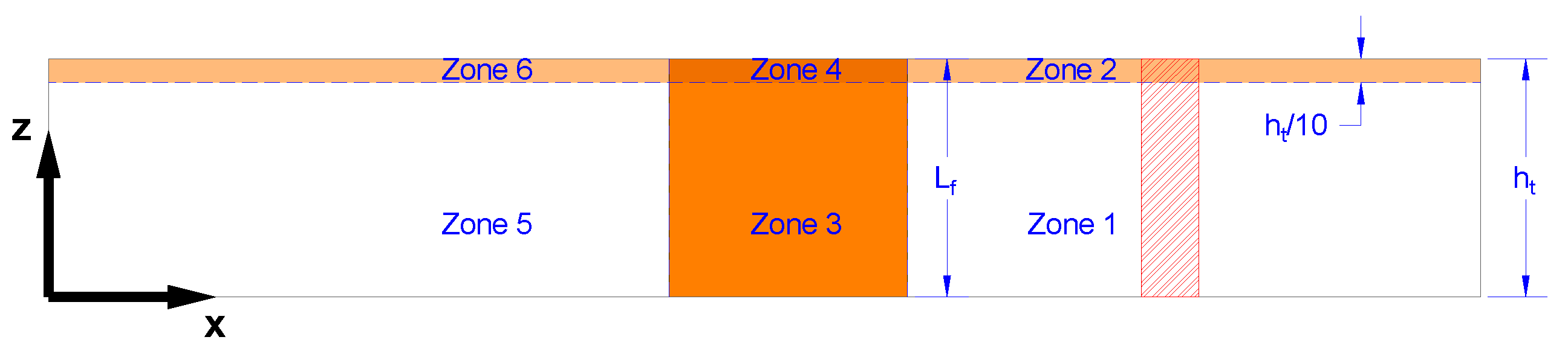
A vertical discretisation is applied to the virtual solid flame to evaluate its temperatures. The floor-to-ceiling distance (along z coordinate) is divided into several layers of identical thickness. The symbol d_z represents the thickness of the layers, while the index k is used to denote the layer number. Layer (1) extends from z = 0 to z = d_z, layer (k) extends from z = (k − 1).d_z to z = k.d_z and so on (see Figure 3). The flame temperature is computed applying the equations from EN1991-1-2 [13], given below in Equations (10)–(12). These equations are based on the model developed by Heskestad [16,17] and Morton [21] and are applied for each layer to evaluate the flame temperature, which is considered as uniform within a given layer.

T(z) = 900 for z < h_base

(10)

T(z) = 20 + 0.25 Q_c^2/3 (z-h_base-z₀)^−5/3 ≤ 900 °C for h_base ≤ z

(11)

where Q_c = 0.8 Q_loc by default and

z₀ = −1.02 D + 0.00524 Q_loc^2/5

(12)

The temperature in the solid flame only depends on the height z. At a given height, it is assumed to be constant in the whole horizontal section of the solid flame. In the developed methodology, the thickness d_z of the layers has to be defined as input, and is rounded down (if needed) to generate layers that all have the same thickness. Knowing the flame length (i.e., height, along z coordinate), the flame is therefore also discretised, following d_z (see Figure 3).

When evaluating the fire geometry and its position in the compartment (see previous section), a time-step dt was introduced, for the only purpose of calculating the related outputs. To evaluate the flame temperature in the compartment, a new time-step Δt is needed, for the purpose of calculating the outputs related to this step and the next one (evaluating the steel temperature of a structural member placed in the compartment). Indeed, the evolution of the flame temperature will be used, along with heat fluxes as described in subsequent sections, to evaluate the evolution of the steel temperature of an (unprotected) structural member following the equation provided in EN1993-1-2 §4.2.5.1 [22], and such equation requires a dedicated time-step of five seconds maximum.

The SFPE handbook [18] states that “fires with very low flame height-to-diameter ratios may generally be expected to produce lower maximum mean temperatures than other fires” but also states that “it is not yet clear whether the type of prediction attempted here for a particular low L/D fire is generally valid”. As the present methodology is intended to evaluate the heating of structural members, the upper bound of the gas temperatures is set to 900 °C, following EN1991-1-2 [13].

2.3.2. Heat Fluxes

Two situations can be encountered: the flame does not impact the ceiling of the compartment, i.e., L_f < h_t (see Figure 4), or the flame does impact the ceiling of the compartment, i.e., L_f ≥ h_t (see Figure 5). Depending on the situation and depending on the location of the target (i.e., where the heat transfer computation for the structural element needs to take place), different zones are defined (see Figure 4 and Figure 5).

The following heat fluxes components will be used (all expressed in W/m²):

• F_r,f refers to the radiative heat flux emitted by the fire surface and received by the structural member;
• F_r,b refers to the radiative heat flux emitted by the surrounding background and received by the structural member;
• F_r,s refers to the radiative heat flux emitted by the structural member;
• F_c refers to the convective heat flux received by the structural member from its surrounding environment;
• F_tot refers to the total net heat flux at the surface of the structural member at a certain height.

Table 1. Heat flux components in Scenario 1.

Scenario 1—The Flame does not Impact the Ceiling of the Compartment
Heat Flux Component	Zone 1	Zone 2	Zone 3	Zone 4	Zone 5	Zone 6
Fr,f	✔	✔			✔	✔
Fr,b,ambient	✔	✔			✔	✔
Fr,b,Heskestad			✔	✔
Fr,b,Hasemi
Fr,s	✔	✔	✔	✔	✔	✔
Fc	✔	✔	✔	✔	✔	✔

and

Table 2. Heat flux components in Scenario 2.

Scenario 2—The Flame Impacts the Ceiling of the Compartment
Heat Flux Component	Zone 1	Zone 2	Zone 3	Zone 4	Zone 5	Zone 6
Fr,f	✔				✔
Fr,b,ambient	✔				✔
Fr,b,Heskestad			✔	✔ *
Fr,b,Hasemi		✔		✔ *		✔
Fr,s	✔	✔	✔	✔	✔	✔
Fc	✔	✔	✔	✔	✔	✔

* Both Heskestad’s and Hasemi’s components are computed but only the maximum value is kept, following the [prEN1991-1-2].

summarize the heat flux components which are considered in the different zones, whilst the formulas to calculate these heat flux components are detailed below.

F_r,f—radiative heat flux emitted by the fire surface and received by the structural member.

The fire is schematised as a rectangular virtual solid flame, and the following equations are based on EN 1991-1-2 Annex G [13] and the outcomes of the RFCS project “LOCAFI” [8]. Referring to the schematic plan view (x,y) depicted on Figure 6, on each face l—with l = 1 to 4—of the rectangular envelope around the steel member at height z_s, the radiative heat flux from an infinitesimal area of the fire surface by an infinitesimal area located at the height of interest on the steel member is computed by Equation (13):

$$d{F}_{r,f,d{A}_1}=\frac{\cos {\theta }_1\cos {\theta }_2}{\pi S_{1-2}^2}\sigma {\epsilon }_f{\epsilon }_m{\left(T_{A_2}+273.15\right)}^{4}d{A}_2$$

(13)

where

• $d{\mathsf{\Phi }}_{d{A}_1-d{A}_2}=\frac{\cos {\theta }_1\cos {\theta }_2}{\pi S_{1-2}^2}d{A}_2$ is the view factor between two infinitesimal areas dA₁ and dA₂ (see EN1991-1-2 equation G.1 [13]);
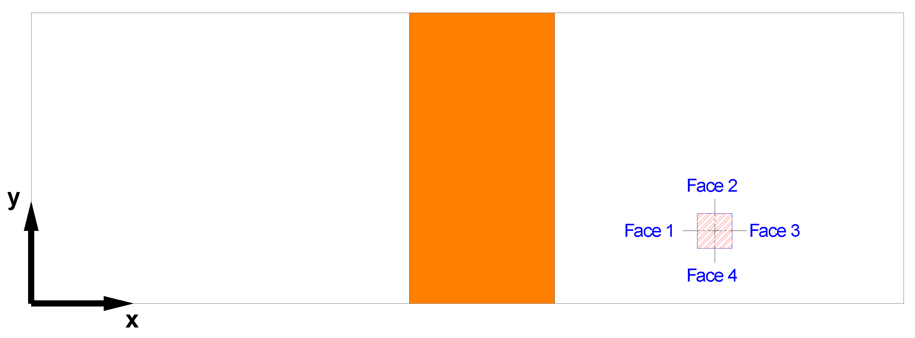
• dA₁ refers to an infinitesimal area on the face l—located at the height of interest on the structural member—which receives the radiative heat flux;
• dA₂ refers to an infinitesimal area on the surface of the solid flame which emits the radiative heat flux;
• T_A2 is the local temperature of the flame at height z_s [°C] (as detailed in previous sub-section);
• σ = 5.67 × 10⁻⁸ is the Stefan–Boltzmann constant [Wm⁻²K⁻⁴];
• ε_m (generally = 0.7) is the surface emissivity of the steel member [-];
• ε_f (generally assumed to be = 1) is the surface emissivity of the flame [-].

The view factor dΦ_A1−A2 measures the fraction of the total radiative heat leaving a given radiating surface that arrives at a given receiving surface. Its value depends on the size of the radiating surface A₂, on the distance from the radiating surface to the receiving surface S₁₋₂ and on their relative orientation (through angles θ₁ and θ₂ between the line that joins both surfaces and their respective normal). The view factor to a member face from which the fire is not visible is taken equal to zero. In the present methodology, the view factor is calculated assuming that each face l is shifted to be localised on the section axis. The total radiative heat flux received by dA₁ from all the fire surfaces is obtained by Equation (14). As the present model assumes that the radiative heat flux F_r,f,A1 is homogeneous on a face l (at the height of interest), the total radiative heat flux received by face l (at the height of interest) is thus computed by Equation (15), where ΔA₂ = Δx. Δy or Δy. Δz depending on the location on the fire surface. The total resulting radiative heat flux F_r,f,tot received from the fire by the steel member at height z_s is computed as the average of the F_r,f,l weighted by the dimensions C_x and C_y of the edges of the steel section envelope, as detailed in Equation (16).

$$F_{r,f,d{A}_1}={{\displaystyle \int }}_{fire surface}^{}\frac{\cos {\theta }_1\cos {\theta }_2}{\pi S_{1-2}^2}\sigma {\epsilon }_f{\epsilon }_m{\left(T_{A_2}+273.15\right)}^{4}d{A}_2$$

(14)

$$F_{r,f,l}={\displaystyle \sum }_{fire surface}\frac{\cos {\theta }_1\cos {\theta }_2}{\pi S_{1-2}^2}\sigma {\epsilon }_f{\epsilon }_m{\left(T_{A_2}+273.15\right)}^4\mathit{\Delta }{A}_2$$

(15)

$$F_{r,f,tot}=\frac{C_x\left(F_{r,f,2}+F_{r,f,4}\right)+C_y\left(F_{r,f,1}+F_{r,f,3}\right)}{2\left(C_x+C_y\right)}$$

(16)

F_r,b—radiative heat flux emitted by the surrounding background and received by the structural member

The radiative heat flux received from the surrounding background by the structural member at height z_s is computed in a different manner depending on the zone where it lies. If the point of interest is situated in ambient air, Equation (17) applies. It corresponds to zones 1, 2, 5, 6 when the flame does not impact the ceiling (see Figure 4), and to zone 1, 5 when the flame impacts the ceiling (see Figure 5). If the point of interest is within the solid flame (i.e., in zone 3 or zone 4), Equation (18) applies, while if it is in the horizontal layer underneath the ceiling when the flame impacts the ceiling (i.e., in zone 2, 4, 6 in Figure 5), Equation (19), as described in EN1991-1-2 [13], applies. These equations, commonly referred as the Hasemi model, are based on experimental tests [23,24,25,26]. Finally, when the flame impacts the ceiling, if the point of interest is in the top layer near the ceiling (zone 4 in Figure 5): the maximum between F_{r,b,Heskestad} and F_r,b,Hasemi is considered, following prEN 1991-1-2:2021 E [27].

$$F_{r,b,ambient}=\sigma {\epsilon }_f{\epsilon }_m{\left(20+273.15\right)}^4$$

(17)

$$F_{r,b,Heskestad}=\sigma {\epsilon }_f{\epsilon }_m{\left(T_{A_2}+273.15\right)}^4$$

(18)

$$F_{r,b,Hasemi}=\left\{\begin{array}{cc}\hfill \mathrm{100,000}\hfill & if y\prime \le 0.30\hfill \\ \hfill \mathrm{136,300}-\mathrm{121,000} y\prime \hfill & if 0.30<y\prime <1.0\hfill \\ \hfill \mathrm{15,000} y{\prime }^{-3.7}\hfill & if y\prime \ge 1.0\hfill \end{array}\right.$$

(19)

Referring to Equation (19):

• y′ is a dimensionless parameter given by

  $$y\prime =\frac{r+\left(h_t-h_{base}\right)+z\prime }{L_h+\left(h_t-h_{base}\right)+z\prime }$$

  (20)
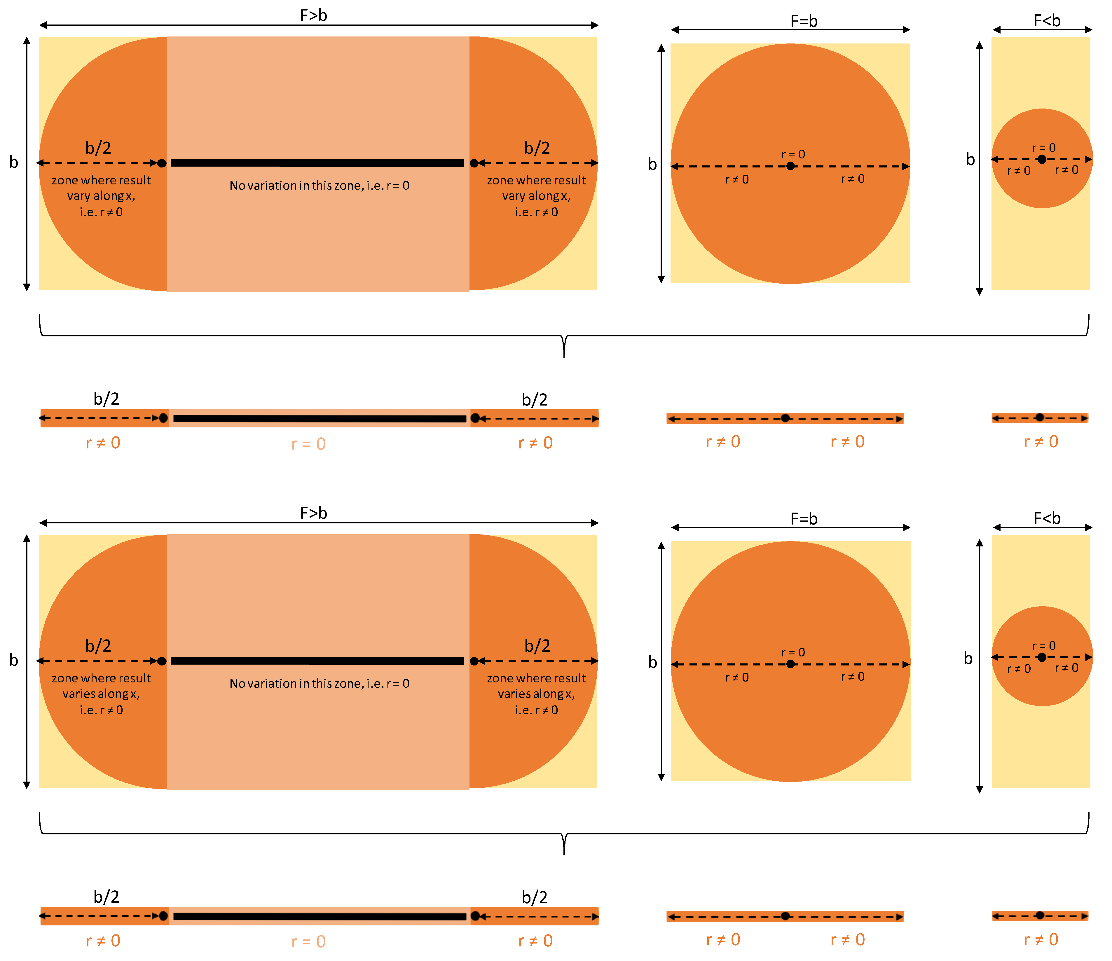
• r is the x-component of the horizontal distance (in m) between the equivalent vertical axis of the fire and the structural member axis, given by the Equation (20) (see Figure 2)

  $$r=\left\{\begin{array}{cc}\left(Backsid{e}_x+\frac{D}{2}\right)-A_x& if A_x<Backsid{e}_x+\frac{D}{2}\\ 0& if Backsid{e}_x+\frac{D}{2}\le A_x\le Frontsid{e}_x-\frac{D}{2}\\ A_x-\left(Frontsid{e}_x-\frac{D}{2}\right)& if Frontsid{e}_x-\frac{D}{2}<A_x\end{array}\right.$$

  (21)
• h_t−h_base is the distance, in m, between the fire source basis and the ceiling
• z′ is the vertical position of the virtual heat source, in m, given by

  $$\begin{array}{}{z}^{\prime }=\left\{\begin{array}{cc}\hfill 2.4D\left(Q_D^{\ast 2/5}-Q_D^{\ast 2/3}\right)\hfill & if Q_D^{\ast }<1.0\hfill \\ \hfill 2.4D\left(1.0-Q_D^{\ast 2/5}\right)\hfill & if Q_D^{\ast }\ge 1.0\hfill \end{array}\right.\\ \mathrm{with}{Q}_D^{\ast }=Q_{loc}/\left({1.11\times 10}^6.D^{2.5}\right)\end{array}$$

  (22)
• L_h is the horizontal flame length, in m, given by

  $$\begin{array}{}{L}_h=2.9\left(ht-h_{base}\right){\left(Q_H^{\ast }\right)}^{0.33}-\left(h_t-h_{base}\right)\\ \mathrm{with}{Q}_H^{\ast }=Q_{loc}/\left({1.11\times 10}^6.{\left(h_t-h_{base}\right)}^{2.5}\right)\end{array}$$

  (23)

The determination of r implies the equivalent vertical axis of the fire. Hasemi’s model is a localised fire model whose thermal action is computed while considering a circular based fire. Any distance from such fire source is then computed from the axis of the circle. In the present methodology, the fire source is assumed to be represented by a rectangular prismatic solid flame, implying a rectangular (or square) based fire. The Hasemi model is generalised as presented in Equations (19)–(23), i.e., by stretching the axis of the fire source onto a whole rectangle. Referring to Figure 7, with b and F being, respectively, the width and the length of the burning area, three cases can be encountered: F > b, F = b, F < b. Actually, when applying Hasemi’s model, the results are only a function of the horizontal distance x (i.e., parallel to the length of the compartment) and the schemes should be represented in 1 dimension, implying that this situation applies whatever the value of y (coordinate parallel to b). As described on Figure 7, in case where F > b, the parameter r is considered equal to zero from b/2 from the fire back and until b/2 before the front.

F_r,s—radiative heat flux emitted by the structural member

The radiative heat flux emitted by the steel member is computed by Equation (24), where T_s is the steel temperature at height z_s, in °C.

$$F_{r,s}=-\sigma {\epsilon }_m{\left(T_s+273.15\right)}^4$$

(24)

F_c—resulting convective heat flux received by the steel member from its surrounding environment

The resulting convective heat flux received by the steel member from its surrounding environment is computed by Equation (25) where α_c, considered equal to 35 Wm⁻²K⁻¹ when natural fire models are used (EN1991-1-2 [13]), is the coefficient of heat transfer by convection and T_g is the gas temperature in the vicinity of the steel member at height z_s, in °C. In zones 1, 2, 5, and 6: T_g is taken as the ambient background temperature (assumed to be at 20 °C), while in zones 3 and 4: T_g is taken as T_A2 (the local temperature of the flame at height z_s, as detailed in previous sub-section, computed through Heskestad model).

$$F_c={\alpha }_c\left(T_g-T_s\right)$$

(25)

F_tot—total resulting heat flux received by the structural member at a certain height

The total resulting heat flux F_tot received by the structural member at height z_s is computed by summing all the previously detailed contribution (see Equation (26)). Equations (24)–(26) are in accordance with EN1991-1-2 [13].

$$F_{tot}=F_{r,f,tot}+F_{r,b}+F_{r,s}+F_c$$

(26)

2.4. Evaluation of the Steel Temperature of a Structural Member Placed in the Compartment

The steel temperature is computed according to EN 1993-1-2 equation 4.25 [22], given below as Equations (27) and (28), respectively. For a given time-step Δt, the Equation (27) allows to compute the corresponding rise in steel temperature ΔT. The following notations are used:

• A_m the surface area of the member per unit length [m²/m];
• V the volume of the member per unit length [m³/m];
• A_m/V the section factor for unprotected steel members [m⁻¹];
• (A_m/V)_b the box value of the section factor (box refers here to the rectangular envelope around the steel member) [m⁻¹];
• c_a the specific heat of steel [Jkg⁻¹K⁻¹] as given in EN1993-1-2 § 3.4.1.2 [22];
• F_tot the design value of the net heat flux per unit area [W/m²];
• Δt the time interval [s];
• ρ_a = 7850 kg/m³ the unit mass of steel.

Once ΔT is known, it is possible to evaluate T_t, the steel temperature at time t through an iterative procedure, see Equation (28).

$$\mathsf{\Delta }T=\frac{{\left(A_m/V\right)}_b}{c_a{\rho }_a}{F}_{tot}\mathsf{\Delta }t$$

(27)

$$T_t=T_{t-1}+\frac{{\left(A_m/V\right)}_b}{c_a{\rho }_a}{F}_{tot}\mathsf{\Delta }t$$

(28)

Since the steel temperature depends on the heat fluxes and that in the present methodology, heat fluxes vary within the compartment (see Figure 4 and Figure 5), the model allows to represent the spatially transient heating of the steel structure. Nevertheless, it assumes a uniform steel temperature for a given cross section, i.e., there is no cross-sectional temperature gradient.

3. Comparison of Steel Temperatures from the Model with Experimental Results

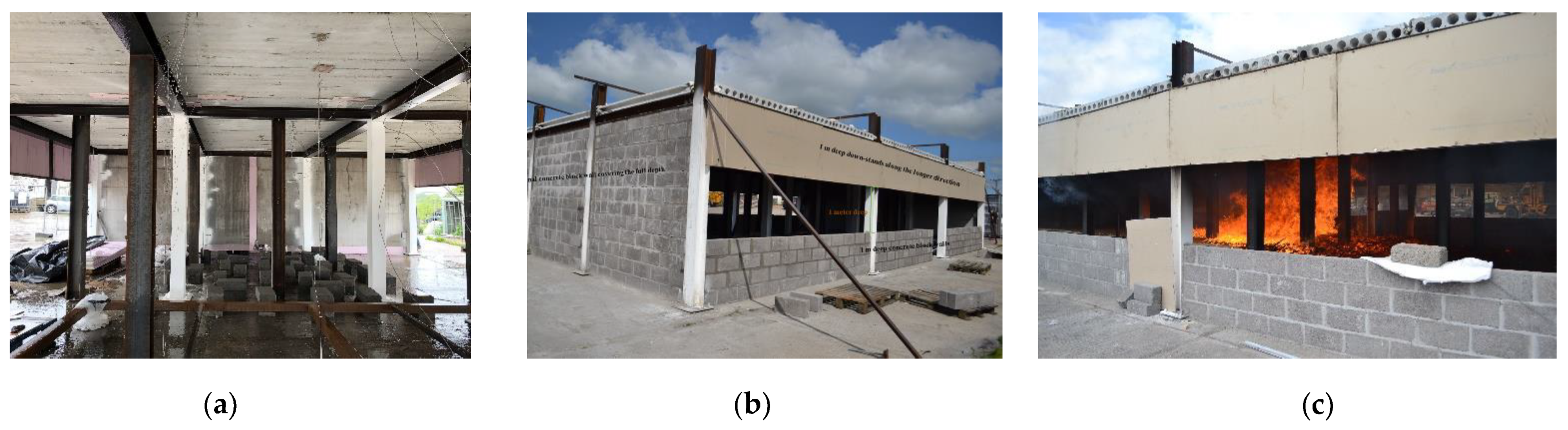
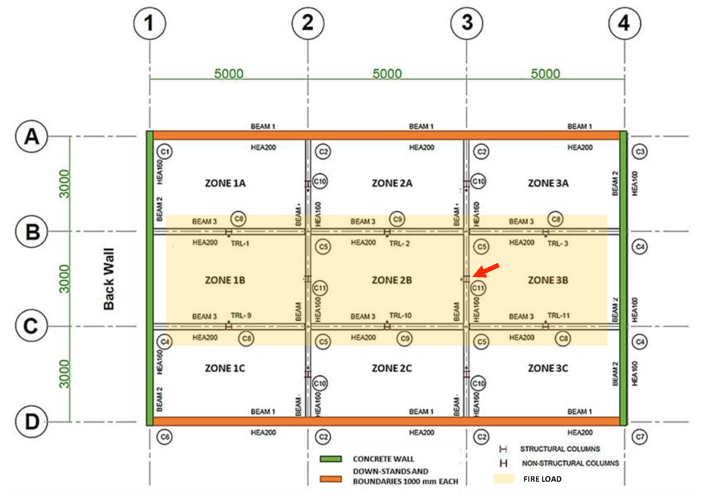
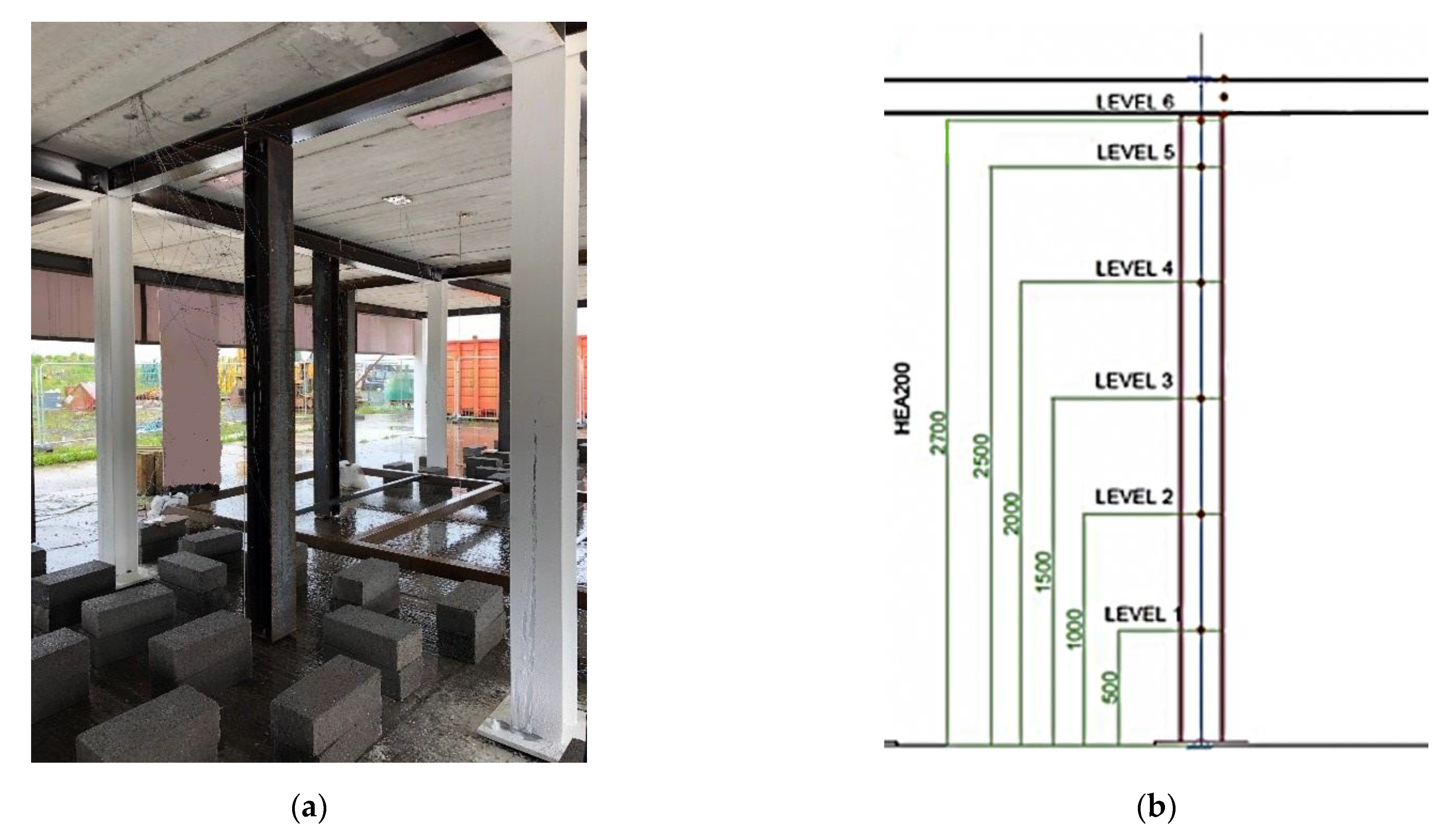
3.1. Experimental Travelling Fire Test in a Steel Building

One of the experimental campaigns of the “TRAFIR” project aimed at performing three large-scale natural fire tests with no artificial control over of the fire dynamics. The main objectives of this experimental campaign were to understand in which conditions a travelling fire develops, as well as how it behaves and impacts the surrounding structure. This paper considers the test n°2, for which a travelling fire occurred (details concerning this experiment can be found in (Alam et al. [28]). The test compartment was designed to represent a part of an entire office layout, consisting of steel beams and columns for the main structural frame (protected ones and unprotected ones for data acquisition purpose, see Figure 8a), while hollow-core precast concrete slabs were used for the ceiling. The layout of the structure can be seen on Figure 9; the floor area is 15 m long and 9 m wide between the outer gridlines while the distance from the surface of the finished floor to the ceiling was 2.9 m. Concrete walls were constructed along the two shorter sides of the compartment (i.e., along gridlines 1 and 4). For the two longer sides (i.e., gridlines A and D), downstands were provided to allow for smoke accumulation below the ceiling as well as a concrete block soffit, such that the openings height is 1 m (along both longer sides). Such configuration provided openings with a total area of 30 m² that were equally distributed along gridlines A and D. Photographs of the compartment can be seen on Figure 8b,c.

A fire load defined according to a well-established methodology (Gamba et al. [29]) was used, consisting of a uniformly distributed fuel wood with a fire load density of 511 MJ/m² arranged in such a way that it would lead to a medium fire propagation (t_α = 300 s, cnfr EN1991-1-2 [13]). The fuel bed is highlighted on Figure 9; it was provided along the centre of the test compartment, in a rectangular band of 14 m-long stretching from wall to wall along the longer dimension of the compartment (a gap of 0.5 m was kept between the short walls and the edge of the fire load). The width of the fuel bed was 4.2 m and was aligned with the centreline of the compartment. The wood sticks were provided on a steel platform located at 325 mm above the floor level. Ignition was at a point located at mid-width of the fire load, 0.5 m from its edge (i.e., at a distance of 1 m from the back wall). The fire started to grow close to gridline 1 and then travelled from gridline 1 to gridline 4.

3.2. Steel Temperatures in Central Columns

During the test, steel temperatures were measured in non-structural unprotected columns. This experimental data is compared with results obtained while applying the analytical method described in this paper: the comparison is performed for the unprotected steel column C11 (highlighted on Figure 9) which is a hot-rolled profile HE 200A.

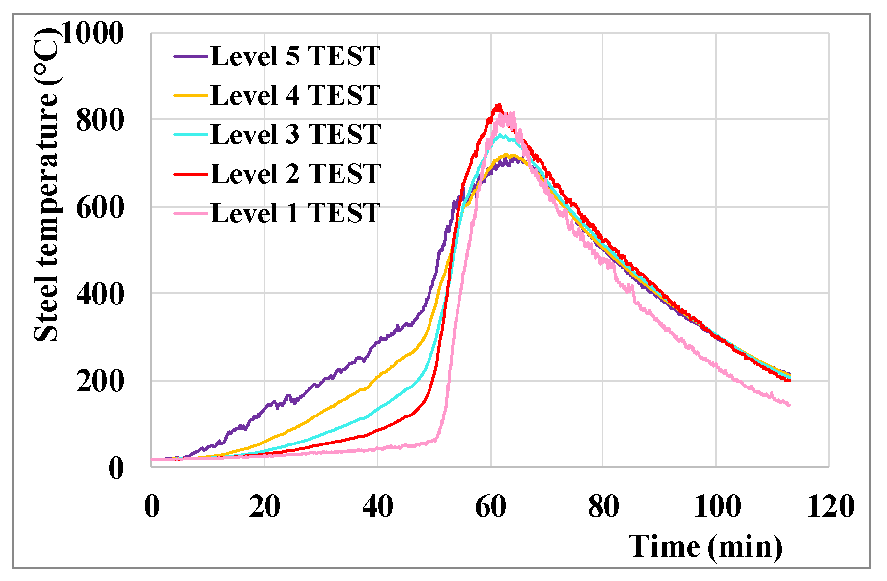
3.2.1. Experimental Measurements

The column C11 is located at mid-width of the compartment and at 10 m from the back wall. Thermocouples were provided at five levels along the height of the column (see Figure 10 where the steel platform and the fire load are still missing). For each level, three thermocouples were placed: one on the web and one on each flange. It was shown by Alam et al. [28] that, whereas there is a temperature gradient along the height of the column, the steel temperature within a given section can be considered as uniform. The experimental data provided below for each level therefore corresponds to the average of the three thermocouples (while the analytical model directly provides a unique steel temperature for a given level).

3.2.2. Comparison of the Results

To apply the model, some input parameters were directly defined from the test set-up:

• The design fire load density q_f,d = 511 MJ/m²;
• The height of the fire load basis h_base = 0.325 m;
• The net heat of combustion of the fire load H was estimated from a bomb calorimeter test (performed by the University of Edinburgh) as 16.8 MJ/kg;
• The total area of vertical openings A_v = 30 m²;
• The equivalent height of the openings h_eq = 1 m.
• Other input parameters were taken from EN 1991-1-2:
• The combustion factor m = 0.8 (leading to an effective heat of combustion = 13.44 MJ/kg);
• The coefficient of convection heat transfer on the steel surface α_c = 35 W/m²K;
• The flame emissivity ε_f = 1;
• The steel emissivity ε_m = 0.7;
• The time-steps dt = Δt = 5 sec.

Finally, three parameters had to be defined based on some assumptions:

• The rate of heat release density RHR_f has been set to 400 kW/m², an evaluation made from the mass loss test measurement;
• Several fire spread rates v were considered and the present comparison was achieved with 3.2 mm/s which is representative of the fire spread rate observed in the first half of the compartment;
• The width of each band was set as d_x = 25 cm (nearly identical results are obtained with a band width of 50 cm);
• The thickness of the flame layers d_z = 10 cm (no sensitivity analysis was carried out for this parameter).

It has to be noted that since the analytical model considers a fire load which is covering the whole floor area of the defined compartment, the compartment length and width were defined as 14 m and 4.2 m, respectively, to match the dimensions of the fire load used in the test. This configuration set up does not influence the criteria which verifies if the fire is air controlled. Indeed, Equation (3) does not depend on the compartment length and width but only on the openings sizes. The width of the two modelled openings is slightly smaller (14 instead of 15 m in the experiment), but this does not influence the results as the fire is not air controlled in both cases (and R is therefore not modified). With the given input data, the time needed to burn the fire load within one band is 1277 s (21 min) while the time needed for the combustion front to cross a band is 78 s.

Figure 11 presents the steel temperatures measured in column C11 at the five different levels while Figure 12 shows the corresponding steel temperatures obtained with the analytical model. On Figure 12, all the curves are overlapping except the one for level 5. Figure 13, Figure 14, Figure 15, Figure 16 and Figure 17 present on common graphs the steel temperature for each level (with the label “TEST” for the experimental data and the label “MODEL” for the results of the analytical model). For the upper levels 4 and 5 (Figure 16 and Figure 17), a third curve “MODEL + ZONE” is plotted, corresponding to the combination of the analytical model with a zone model. Indeed, such combination is needed to properly capture the effect of the hot smoke layer below the ceiling. In this case, the software OZone (Cadorin [30]) was applied, modelling the real compartment volume and the evolution of the fire as the one from the analytical procedure (i.e; the 4.2 m width band-by-band evolution with time). This combination was computed for level 5 (implying a smoke layer of at least 40 cm) and for level 4 (implying a smoke layer of at least 90 cm). When combination is considered, the maximum steel temperature of both calculation methods is plotted.

4. Discussion and Application Field of the Model

The following observations can be made from the Figure 13, Figure 14, Figure 15, Figure 16 and Figure 17:

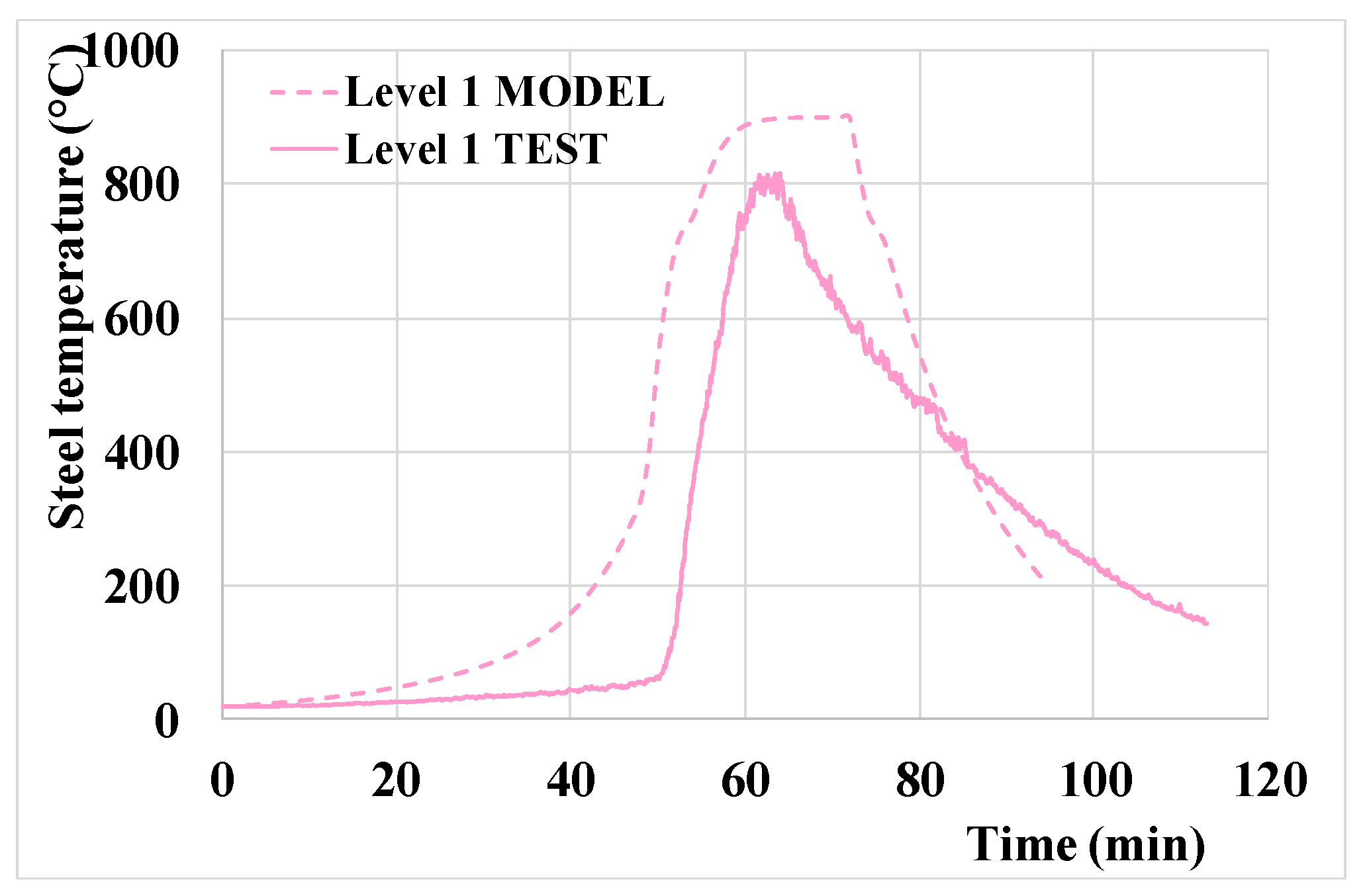
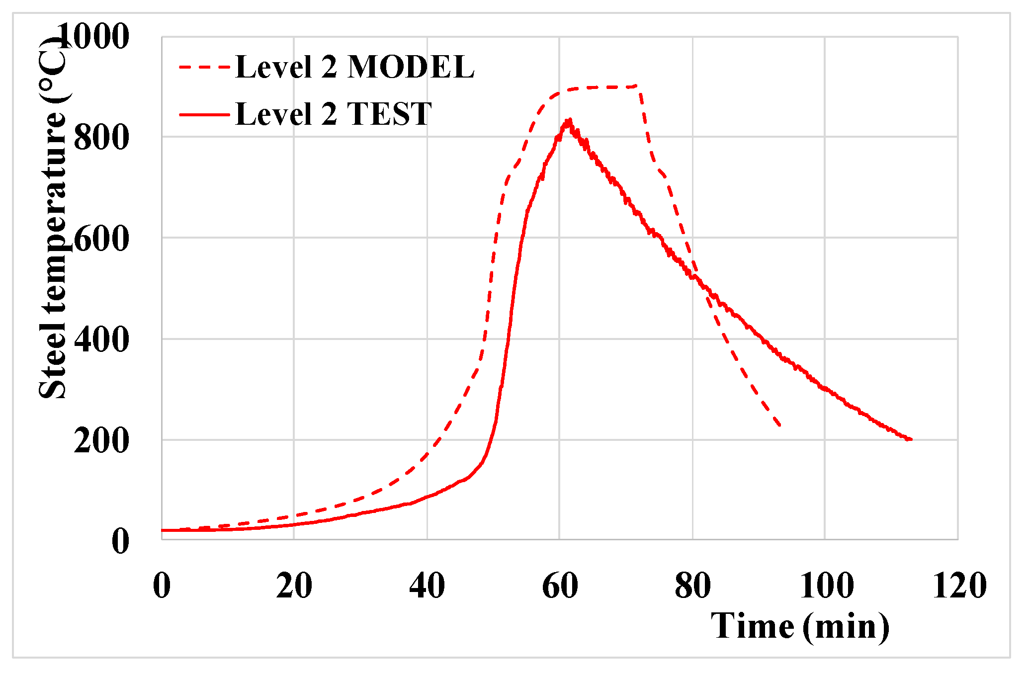
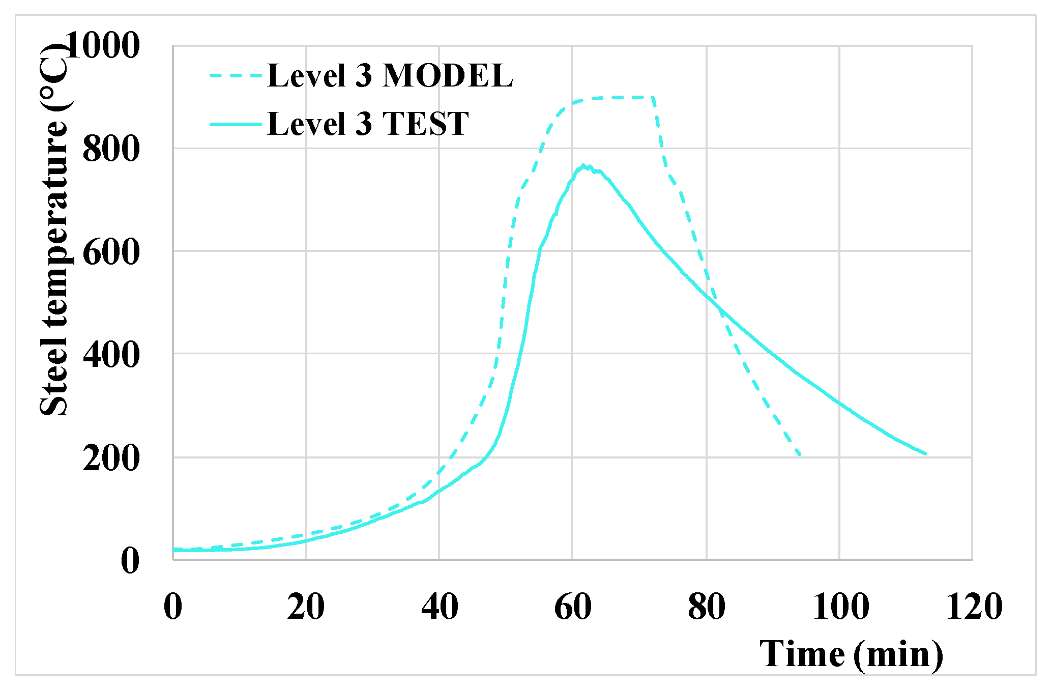
• The global profile versus time is well captured;
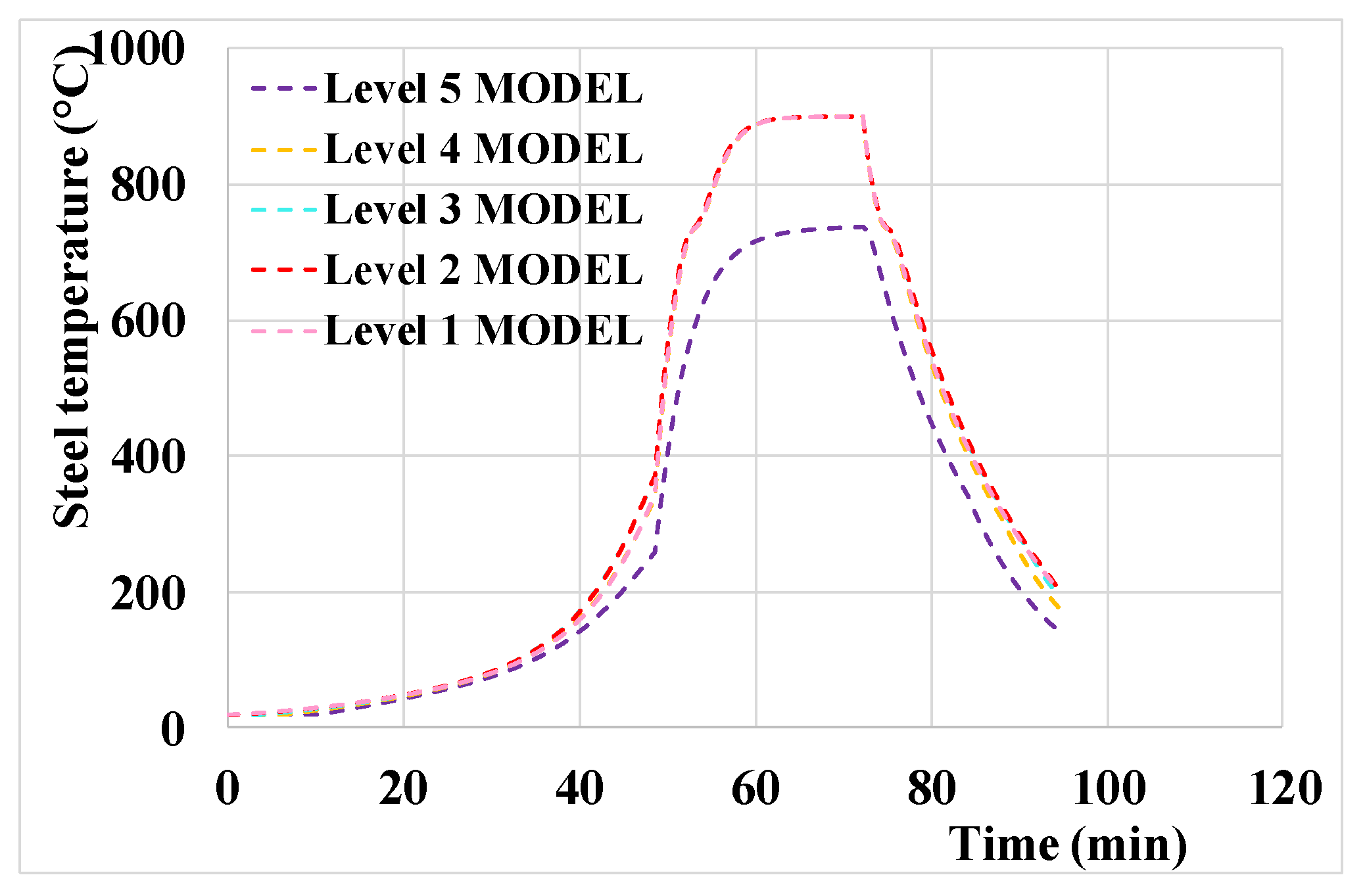
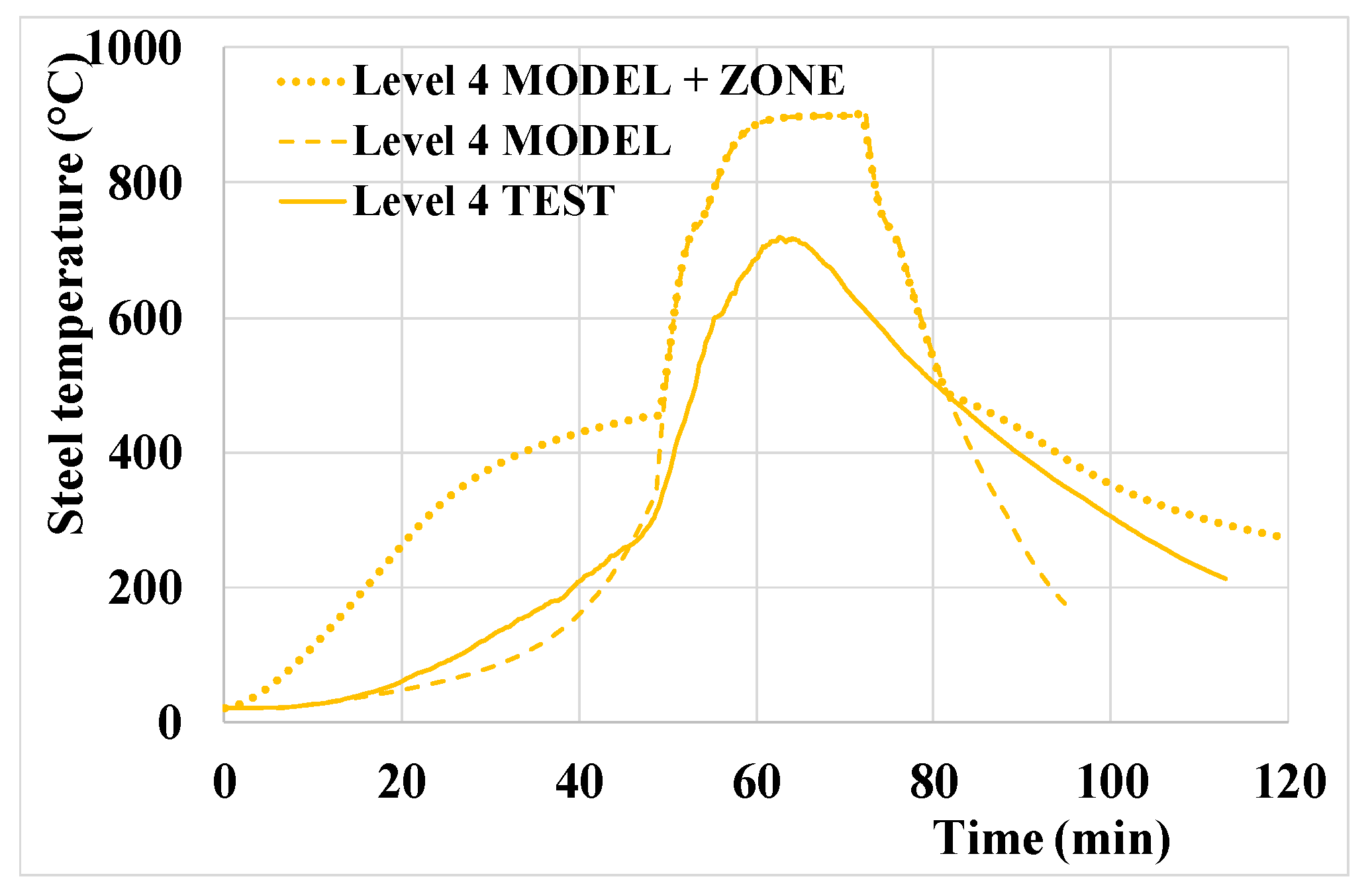
• The obtained steel temperatures are safe-sided for all levels. The peak temperatures are quite close to the ones measured during the test, except for mid-levels (3 and 4) where a non-negligible difference is found: for levels 1 and 2 the difference is around 90 °C (900 °C for the model versus 810 °C for the test). For levels 3 and 4 the difference is around (respectively) 150 and 190 °C (900 °C for the model versus, respectively, 750 and 710 °C for the test). For level 5, the peak temperature is similar, around 710 °C;
• The time during which the steel temperatures are high (i. e. above 500 °C—threshold arbitrarily chosen in a domain where the yield strength of steel has started to decrease) is slightly longer for the model than for test at levels 1, 2 and 3 (around 27 min for the test and 30 min for the model). However, for levels 4 and 5 a very good match is observed with 30 min for both the model and the test;
• However, for steel temperatures above 700 °C (temperature for which the yield strength of steel has significantly decreased) the difference is more important. With the model, steel temperatures are above 700 °C during 25 min for levels 1, 2, 3 and 4 and 15 min for level 5 while for the test this duration is approximately 10 min for levels 1 and 3, 12 min for level 2 and 5 min for levels 4 and 5;
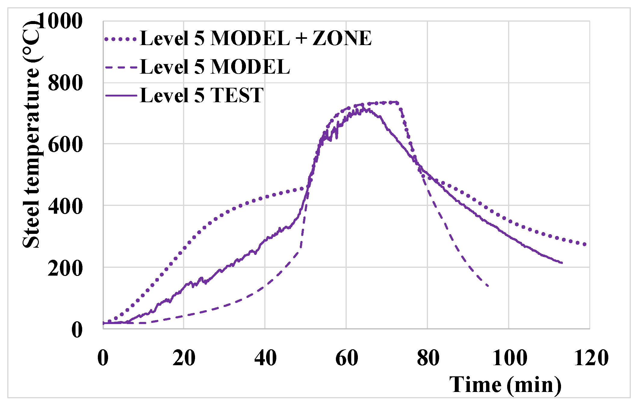
• The developed model considers only the effect of the spreading localised fire, and needs to be coupled to a zone model for the upper levels to consider the hot gases which develop under the ceiling. For the highest level (level 5 which is located 40 cm below the ceiling), the application of the model only leads to unsafe results for the heating branch and to a good representation of the peak temperatures. The combination with a zone model allows to improve the representation of the fire; the peak temperatures are unchanged, but the heating branch is better captured with safe-sided results. For the level 4, which is located 90 cm below the ceiling, the application of the model only leads to slightly unsafe results for the heating branch and to significantly safe-sided results for the peak temperatures. The combination with a zone model leads to significantly safe-sided results for both the heating branch and the peak temperatures (which are unchanged);
• The descending branch is underestimated once steel temperatures goes below 400 °C. Such issue was also noticed through CFD numerical modelling (Charlier et al., 2021); this can be explained by the model’s inability to properly capture heat release from glowing embers, as well as the heat accumulated within the compartment boundaries.

The present methodology has some limitations, some of them being directly linked to simplifications which have to be made in the frame of an analytical procedure. Obvious limitations are linked to the main basic assumptions of the model: the enclosure is rectangular (therefore not allowing for complex geometries—or necessitating to simplify them), the fire path is one-dimensional and the fire load is uniformly distributed on the floor area (while in reality, if some part of the compartment floor is free of fire load, it will not be subjected to the same heat fluxes). Furthermore, the effects of the boundary conditions on the fire plume are disregarded. Therefore, the exact location of the openings is not considered, making impossible the consideration of local effects (for example deceleration followed by acceleration of the fire when reaching an isolated opening, as shown by Charlier et al. [3]). It is important to highlight that the present analytical model is only applicable to represent travelling fire scenarios. It does not allow to automatically transition to flashover and is not appropriate to represent fully developed compartment fires. In the frame of the “TRAFIR” project (Charlier et al. [31]), CFD parametric analyses were performed to better understand in which conditions a travelling fire would develop; applying this analytical model amounts to consider that a travelling fire is developping. Hidalgo et al. [32] proposed a three modes classification of the fire dynamics based on the ratio of flame spread velocity and burnout front velocity: “fully developed”, “growing” and “travelling”. Gupta et al. [33] precise heat fluxes criteria allowing to distinguish between them; the “travelling” mode occurs when enclosure heat losses are important enough such that the pre-heating by the external heat flux ahead of the flame front is minimal. Several modifications can therefore be brought to improve the proposed analytical procedure. Some of these may be deemed as possible for an analytical approach (for example: multi directional fire spread), but others may be dealt with only through the use of numerical tools (for example: automatic transition to flashover and consideration of the exact location and evolution of the openings). In both cases, the authors would like to encourage further work on this topic to improve the proposed procedure. The authors would like to point out that this methodology is not aimed at performing detailed analysis of the local fire dynamics; it is aimed at evaluating the structural response (i.e., heating of the structural elements, followed by a mechanical analysis) in a compartment subjected to travelling fire.

5. Conclusions

The article presents the development of an analytical model to determine the heat fluxes to a structural element due to a travelling fire for (pre-)design purposes. The methodology is based on localised fire models, generalised to the situation when the fire travels across the whole enclosure. The influence of the openings is considered through a simple concept based on the openings size to consider the ventilation limitation. This paper shows that combining the concept of virtual solid flame with a zone model (representing hot gases at upper levels) allows to capture the transient heating of the structural elements.

The proposed methodology allows overcoming some of the limitations from existing analytical methods, but remains based on some simple considerations which are described (some being inherent to the analytical character of the model). The procedure is only applicable to represent travelling fire scenarios: it does not allow to automatically transition to flashover and is not appropriate to represent fully developed compartment fires.

The proposed formulas have been experimentally verified in a full-scale natural fire experiment, and the comparisons are encouraging; one of the “TRAFIR” natural fire tests is modelled and steel temperatures measured on a central steel column are compared. The steel temperature profiles globally showed a good correspondence with those of the test, showing a conservative agreement except for the descending branch which can be explained by the model’s inability to properly capture heat release from glowing embers, as well as the release of heat accumulated within the compartment boundaries. In conclusion, this analytical model represents a valuable tool to be potentially used in the design practice for structural fire engineering applications involving travelling fire scenarios, as well as a robust basis for further research in the field.

References

1. Horová, K. Modelling of Fire Spread in Structural Fire Engineering. Ph.D. Thesis, Czech Technical University in Prague, Prague, Czechia, 2015. [Google Scholar]
2. Degler, J.; Eliasson, A.; Anderson, J.; Lange, D.; Rush, D. A-priori modelling of the Tisova fire test as input to the experimental work. In Proceedings of the 1st International Conference on Structural Safety under Fire & Blast, Glasgow, UK, 2–4 September 2015. [Google Scholar]
3. Charlier, M.; Gamba, A.; Dai, X.; Welch, S.; Vassart, O.; Franssen, J.-M. CFD analyses used to evaluate the influence of compartment geometry on the possibility of development of a travelling fire. In Proceedings of the 10th International Conference on Structures in Fire, Ulster University, Belfast, UK, 6–8 June 2018; pp. 341–348. [Google Scholar]
4. Charlier, M.; Glorieux, A.; Dai, X.; Alam, N.; Welch, S.; Anderson, J.; Vassart, O.; Nadjai, A. Travelling fire experiments in steel-framed structure: Numerical investigations with CFD and FEM. J. Struct. Fire Eng. 2021, 12, 309–327. [Google Scholar] [CrossRef]
5. Dai, X.; Welch, S.; Rush, D.; Charlier, M.; Anderson, J. Characterising natural fires in large compartments—Revisiting an early travelling fire test (BST/FRS1993) with CFD. In Proceedings of the 15th International Interflam Conference, London, UK, 1–3 July 2019. [Google Scholar]
6. Stern-Gottfried, J.; Rein, G. Travelling fires for structural design-Part II: Design methodology. Fire Saf. J. 2012, 54, 96–112. [Google Scholar] [CrossRef] [Green Version]
7. Rackauskaite, E.; Hamel, C.; Law, A.; Rein, G. Improved Formulation of Travelling Fires and Application to Concrete and Steel Structures. Struct. 2015, 3, 250–260. [Google Scholar] [CrossRef] [Green Version]
8. Vassart, O.; Hanus, F.; Brasseur, M.; Obiala, R.; Franssen, J.-M.; Scifo, A.; Zhao, B.; Thauvoye, C.; Nadjai, A.; Sanghoon, H. LOCAFI: Temperature Assessment of a Vertical Steel Member Subjected to Localised Fire—Final Report, Research Fund for Coal and Steel; European Commission: Brussels, Belgium, 2016. [Google Scholar]
9. Tondini, N.; Thauvoye, C.; Hanus, F.; Vassart, O. Development of an analytical model to predict the radiative heat flux to a vertical element due to a localised fire. Fire Saf. J. 2019, 105, 227–243. [Google Scholar] [CrossRef]
10. Dai, X.; Welch, S.; Vassart, O.; Cábová, K.; Jiang, L.; Maclean, J.; Clifton, G.C.; Usmani, A. An extended travelling fire method framework for performance-based structural design. Fire Mater. 2020, 44, 437–457. [Google Scholar] [CrossRef]
11. Janssens, M.L. An Introduction to Mathematical Fire Modeling, 2nd ed.; CRC Press: Lancaster, PA, USA, 2000. [Google Scholar]
12. Kawagoe, K. Fire Behaviour in Rooms; Report of the Building Research Institute: Ibaraki-ken, Japan, 1958. [Google Scholar]
13. CEN (European Committee for Standardization). EN1991-1-2: Eurocode 1: Actions on Structures—Part 1–2: General Actions—Actions on Structures Exposed to Fire; CEN: Brussels, Belgium, 2002. [Google Scholar]
14. Zukoski, E.; Kubota, T.; Cetegen, B. Entrainment in fire plumes. Fire Saf. J. 1981, 3, 107–121. [Google Scholar] [CrossRef]
15. Merci, B.; Beji, T. Fluid Mechanics Aspects of Fire and Smoke Dynamics in Enclosures; CRC Press: Boca Raton, FL, USA; Balkena: Amsterdam, The Netherlands, 2016. [Google Scholar]
16. Heskestad, G. Luminous heights of turbulent diffusion flames. Fire Saf. J. 1983, 5, 103–108. [Google Scholar] [CrossRef]
17. Heskestad, G. Engineering relations for fire plumes. Fire Saf. J. 1984, 7, 25–32. [Google Scholar] [CrossRef]
18. SFPE Handbook of Fire Protection Engineering, 3rd ed.; NFPA: Quincy, MA, USA, 2002.
19. Randaxhe, J.; Popa, N.; Tondini, N. Probabilistic fire demand model for steel pipe-racks exposed to localised fires. Eng. Struct. 2021, 226, 111310. [Google Scholar] [CrossRef]
20. McCaffrey, B. The SFPE Handbook of Fire Protection Engineering, 2nd ed.; Society of Fire Protection Engineers and National Fire Protection Association: Quincy, MA, USA, 1995. [Google Scholar]
21. Morton, B.R. Modeling of fire plumes. In Proceedings of the 10th International Symposium on Combustion; The Combustion Institute: Pittsburgh, PA, USA, 1965. [Google Scholar]
22. CEN (European Committee for Standardization). EN1993-1-2: Eurocode 3: Design of Steel Structures—Part 1–2: General Rules—Structural Fire Design; CEN: Brussels, Belgium, 2005. [Google Scholar]
23. Hasemi, Y.; Tokunaga, T. Flame Geometry Effects on the Buoyant Plumes from Turbulent Diffusion Flames. Fire Sci. Technol. 1984, 4, 15–26. [Google Scholar] [CrossRef] [Green Version]
24. Pchelintsev, A.; Hasemi, Y.; Wakarnatsu, T.; Yokobayashi, Y.; Wakamatsu, T. Experimental and Numerical Study On The Behaviour of A Steel Beam Under Ceiling Exposed to A Localized Fire. Fire Saf. Sci. 1997, 5, 1153–1164. [Google Scholar] [CrossRef] [Green Version]
25. Hasemi, Y.; Yokobayashi, Y.; Wakamatsu, T.; Ptchelintsev, A. Fire Safety of Building Components Exposed to a Localized Fire—Scope and Experiments on Ceiling/Beam System Exposed to a Localized Fire; Interscience Communications: Gosport, Hampshire, UK, 1995. [Google Scholar]
26. Wakamatsu, T.; Hasemi, Y.; Yokobayashi, Y.; Ptchelintsev, A. Experimental Study on the Heating Mechanism of a Steel Beam under Ceiling exposed to a localized Fire. In Proceedings of the 7th Interflam Conference, Cambridge, UK, 26–28 March 1996; pp. 509–518. [Google Scholar]
27. CEN (European Committee for Standardization). prEN 1991-1-2:2021 E: Eurocode 1: Actions on Structures—Part 1-2: General Actions—Actions on Structures Exposed to Fire; CEN: Brussels, Belgium, 2021. [Google Scholar]
28. Alam, N.; Nadjai, A.; Charlier, M.; Vassart, O.; Welch, S.; Sjöström, J.; Dai, X. Large-Scale-Travelling-Fire-Tests with Open-Ventilation-Conditions and Their Effect on the Surrounding Steel-Structure—The-Second-Fire-Test. J. Constr. Steel Res. Under Review.
29. Gamba, A.; Charlier, M.; Franssen, J.-M. Propagation tests with uniformly distributed cellulosic fire load. Fire Saf. J. 2020, 117, 103213. [Google Scholar] [CrossRef]
30. Cadorin, J.-F.; Franssen, J.-M. A tool to design steel elements submitted to compartment fires—OZone V2. Part 1: Pre- and post-flashover compartment fire model. Fire Saf. J. 2003, 38, 395–427. [Google Scholar] [CrossRef]
31. Charlier, M.; Franssen, J.-M.; Temple, A.; Welch, S.; Nadjai, A. Characterization of Travelling Fires in Large Compartments (TRAFIR); European Commission: Brussels, Belgium, 2021; Technical steel research, Draft Final Report (under review). [Google Scholar]
32. Hidalgo, J.P.; Cowlard, A.; Abecassis-Empis, C.; Maluk, C.; Majdalani, A.; Kahrmann, S.; Hilditch, R.; Krajcovic, M.; Torero, J. An experimental study of full-scale open floor plan enclosure fires. Fire Saf. J. 2017, 89, 22–40. [Google Scholar] [CrossRef]
33. Gupta, V.; Osorio, A.F.; Torero, J.L.; Hidalgo, J.P. Mechanisms of flame spread and burnout in large enclosure fires. Proc. Combust. Inst. 2021, 38, 4525–4533. [Google Scholar] [CrossRef]
Figure 1. Simplified representation of the compartment to apply the analytical model.
Applsci 11 09263 g001
Figure 2. Length of the combustion area.
Applsci 11 09263 g002
Figure 3. Vertical discretisation of the virtual solid flame.
Applsci 11 09263 g003
Figure 4. Zones for fire model if the flame does not impact the ceiling.
Applsci 11 09263 g004
Figure 5. Zones for fire model if the flame impacts the ceiling.
Applsci 11 09263 g005
Figure 6. Plan view (x,y) of the compartment: faces of the steel element (rectangular envelope).
Applsci 11 09263 g006
Figure 7. Model of the virtual solid flame: 3 cases (linear scheme according to x coordinate).
Applsci 11 09263 g007
Figure 8. Photographs of the experimental campaign carried out by Ulster University in the frame of “TRAFIR” project: (a) steel frame with protected and unprotected columns; (b) compartment for test n°2; (c) fire at around mid-length of the compartment during test n°2.
Applsci 11 09263 g008
Figure 9. Layout plan of the test compartment, of the fire load and of the steel columns with considered column C11 highlighted (dimensions in mm) [28].
Applsci 11 09263 g009
Figure 10. Photographs of the large scale natural fire tests carried out by Ulster University in the frame of “TRAFIR” project: (a) unprotected steel column with thermocouples; (b) levels of the thermocouples.
Applsci 11 09263 g010
Figure 11. Test n°2—Steel temperature in column C11 at different levels.
Applsci 11 09263 g011
Figure 12. Analytical model—Steel temperature at different levels.
Applsci 11 09263 g012
Figure 13. Steel temperature—Test n°2 versus analytical model at level 1.
Applsci 11 09263 g013
Figure 14. Steel temperature—Test n°2 versus analytical model at level 2.
Applsci 11 09263 g014
Figure 15. Steel temperature—Test n°2 versus analytical model at level 3.
Applsci 11 09263 g015
Figure 16. Steel temperature—Test n°2 versus analytical model and analytical model combined with zone model at level 4.
Applsci 11 09263 g016
Figure 17. Steel temperature—Test n°2 versus analytical model and analytical model combined with zone model at level 4.
Applsci 11 09263 g017