The Application of a Linear Microphone Array in the Quantitative Evaluation of the Blade Trailing-Edge Noise Reduction

Abstract

This paper concerns the application of a linear microphone array in the quantitative evaluation of blade trailing-edge (TE) noise reduction. The noise radiation from the blades with straight and serrated TEs is measured in an indoor open-jet wind tunnel. The array data are processed using the inverse method based on the Clean algorithm based on spatial source coherence (Clean-SC). In order to obtain correct application and achieve the best effect for the microphone array test, the computing software for array data reduction is firstly developed and assessed by Sarradj’s benchmark case. The assessment results show that the present array data processing method has a good accuracy with an error less than 0.5 dB in a wide frequency range. Then, a linear array with 32 microphones is designed to identify the noise source of a NACA65(12)-10 blade. The performance of the Clean-SC algorithm is compared with the Clean algorithm based on point spread functions (Clean-PSF) method for experimentally identifying the noise sources of the blade. The results show that there is about a 2 dB error when using the Clean-PSF algorithm due to the interference of different aerodynamic noise sources. Experimental studies are conducted to study the blade TE noise reduction using serrated TEs. The TE noise for the blade with and without sawtooth configurations is measured with the flow speeds from 20 m/s to 70 m/s, and the corresponding Reynolds numbers based on the chord are from 200,000 to 700,000. Parametric studies of the sawtooth amplitude and wavelength are conducted to understand the noise reduction law. It is observed that the TE noise reduction is sensitive to both the amplitude and wavelength. The flow speed also affects the noise reduction in the serrated TEs. To obtain the best noise suppression effect, the sawtooth configuration should be carefully designed according to the actual working conditions and airflow parameters.

1. Introduction

Turbulence broadband noise from the trailing-edge (TE) and leading-edge (LE) of an airfoil/blade is an important and challenging problem in aeroacoustics [1]. The TE noise comes from the interaction between the fluctuating pressure in the turbulent boundary layer and the sharp TE. As a typical aerodynamic noise source, TE noise has been widely studied. Since the theoretical work of Curle [2], considerable progress has been made towards a clarification of various surface effects. The first essential results and theoretical understanding of the TE noise are from Ffowcs Williams and Hall [3]. By solving the Lighthill’s acoustic analogy equation with an appropriate Green’s function, they found that the far-field sound intensity of the TE noise follows the fifth law with the inflow velocity. After Ffowcs Williams and Hall, many researchers worked on edge noise to understand and predict this noise, such as Crighton and Leppington [4], Crighton [5], Chandiramani [6], Levine [7], Howe [8,9], Chase [10,11], Davis [12], and Howe [13]. Based on the above theoretical studies, the TE noise was also studied experimentally by Brooks et al. [14,15] and modeled analytically by Amiet [16,17] and Howe [18].

The TE noise reduction has been an important focus for many years [19]. The silent flying owls provide great inspiration for aeronautical scientists to design quieter vehicles [20,21]. Inspired by the quiet flying owls, porous modifications [22,23,24] and flexible brushes [25] have been used for noise reduction. In this study, we use another noise reduction treatment named serrated TEs which have been initially modeled by Howe [26,27]. Both sinusoidal [26] and sawtooth TEs [27] were theoretically studied by Howe, and considerable noise reduction was obtained for both treatments. After Howe’s work, many experimental investigations were conducted to explore the noise benefits of the serrated TEs, and the serrated treatments were proved to be an effective noise control configuration [28,29]. However, it was found that Howe’s serration model over-predicts the noise reduction effect in the high-frequency range, while it under-predicts the noise reduction effect in the low-frequency range [30].

It is proposed that the flow and acoustic mechanism of the realistic airfoil and turbomachinery blade are more sophisticated than that of the semi-infinite plane used by Howe due to the loading distribution and the flow turning. Especially, there is a complicated interrelationship between the LE flow and TE flow for the realistic blade due to the small chord [30]. The LE and TE noise sources always arise simultaneously, and these two sources are always very close to each other. In order to explore the noise generation mechanism of LE and TE noise, and to assess the noise reduction effect of the noise control treatments, it is necessary to separate and quantify the airfoil LE and TE noise source. In particular, this is because most of the aerodynamic and performance tests are carried out in the non-anechoic indoor test bed, and not all aeroacoustic tests can be done in a perfect anechoic chamber. There exists very strong background noise which can contaminate the LE and TE noise in these tests. Therefore, it would be critical to separate and quantify the airfoil LE and TE noise source to get the useful aeroacoustic information.

Acoustic beamforming using a phased microphone array is a widely used method and powerful technique to characterize and localize the flow-induced noise. The performance of the beamforming mainly depends on the array distribution and the data reduction method. The accurate strength of the sound source can be determined due to the recent development of the inverse method [31,32,33,34,35]. Deconvolution methods, which aim to identify the point spread functions (PSF) of source maps, may fail when the actual beam patterns of the sound source are not similar to the synthetic PSF. To resolve this problem, a new deconvolution method named Clean based on spatial source coherence (Clean-SC) is developed. The side lobes can be removed using the Clean-SC algorithm. One important advantage of the Clean-SC method is that it can be used to extract the absolute sound levels from the sound maps [36].

This study concerns the quantitative evaluation of the blade TE noise reduction with serrated TEs based on the Clean-SC algorithm. The computing software for microphone array data processing is developed and assessed by Sarradj’s benchmark case. A linear array with 32 microphones is employed to identify the LE noise and TE noise of a blade. The TE noise for the blade with and without sawtooth configurations is measured with various inflow velocities. Parametric studies of the sawtooth amplitude and wavelength on TE noise reduction are performed to systematically explore the noise reduction performance.

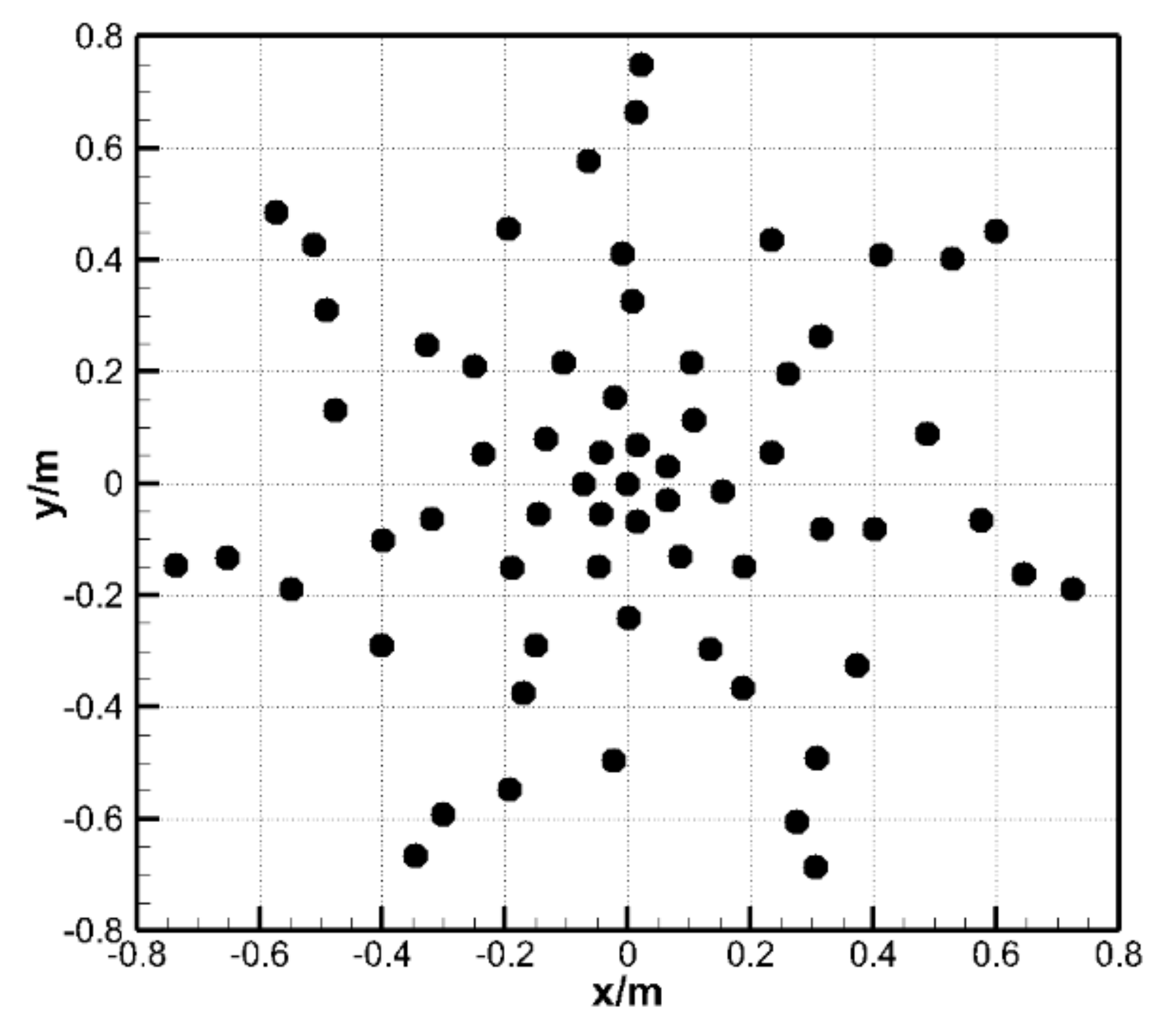
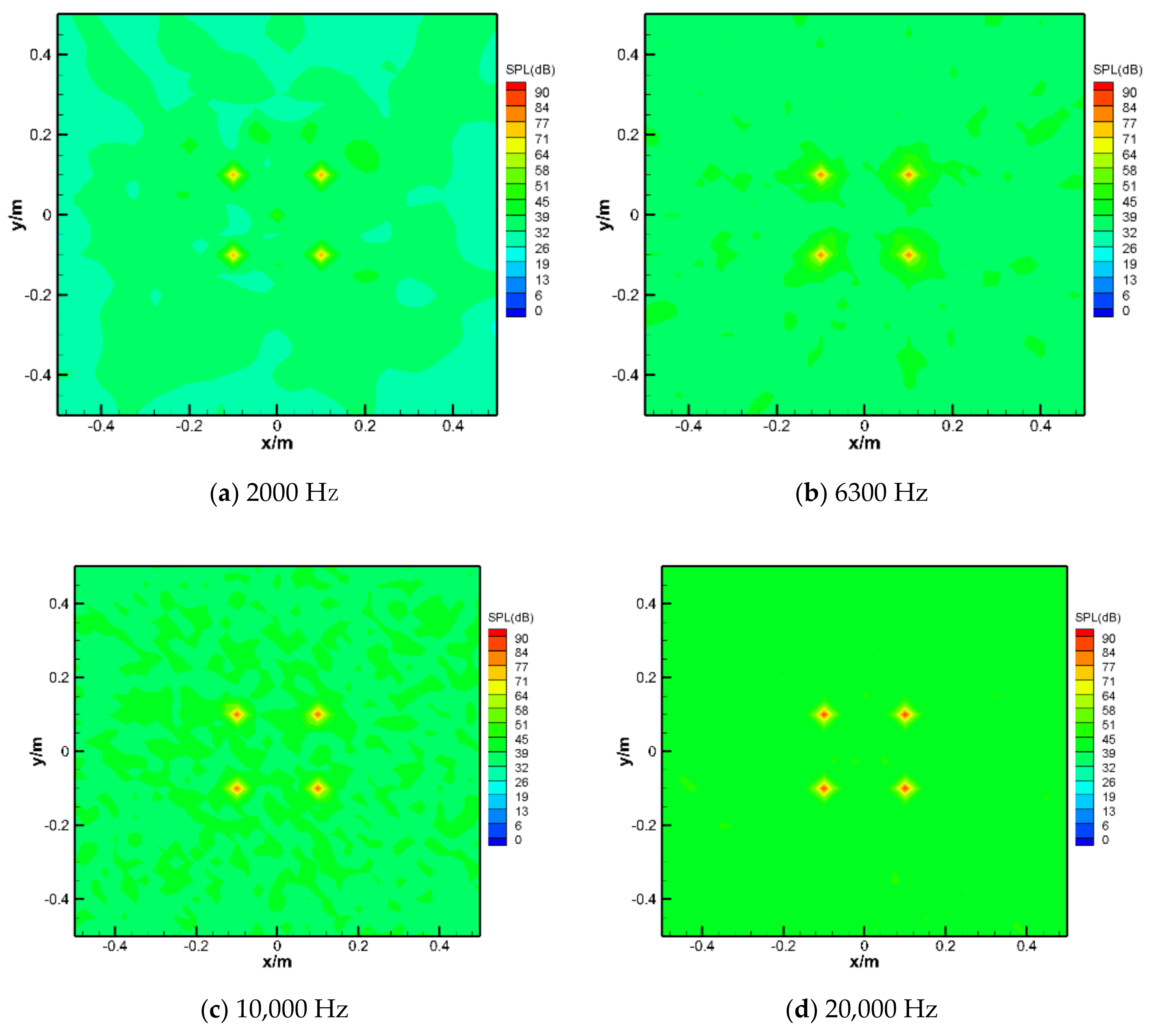
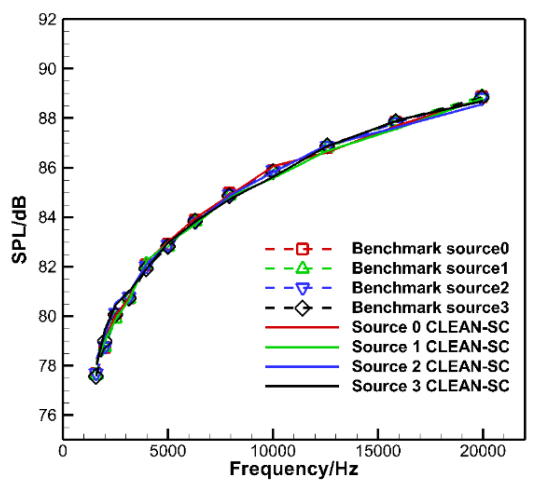
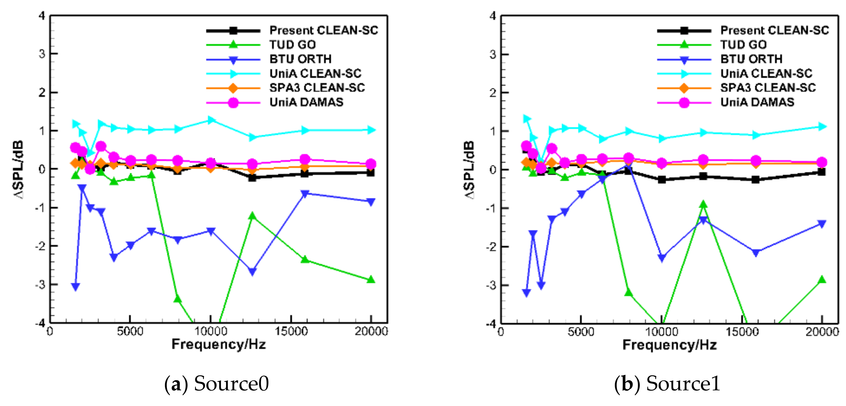
2. The Assessment of the Array Data Processing Software Using Sarradj’s Benchmark Synthesized Input Data

The benchmark synthesized input data proposed by Sarradj et al. [37] are used to assess the present array data reduction program which is based on the Clean-SC algorithm. The Clean-SC is an improved version of the classical deconvolution method Clean [38] employed in Astronomy. It was proposed to overcome the disadvantages of PSF-based methods and it takes advantage of the fact that the main-lobes are spatially coherent with their side-lobes. The beam pattern of each noise source was determined by solving the measured spatial coherence rather than by using the synthetic PSF’s. Better noise identification results might be achieved by Clean-SC compared with other deconvolution methods such as DAMAS [34], due to the fact that Clean-SC does not assume theoretical beam patterns. In addition, Clean-SC is an efficient deconvolution method which takes only twice the data-processing time for conventional beamforming [36].

The benchmark synthesized input data include four monopole sound sources located at the four corners of a square with dimensions of 0.2 m × 0.2 m. The sources are 0.75 m away from the planar array with sixty-four microphones. The exact coordinates of the sources are, respectively, 0.1 m, −0.1 m, 0.75 m; −0.1 m, −0.1 m, 0.75 m; −0.1 m, 0.1 m, 0.75 m and 0.1 m, 0.1 m, 0.75 m. As shown in Figure 1, the planar array has approximately a 1.5 m aperture with seven spiral arms. We evaluate two subcases in this study. For subcase A, the four sources possess the same sound intensity. For subcase B, the four sources possess different intensity with the other three sources respectively having sound levels of 6 dB, 12 dB and 18 dB less than the most intensive source.

As indicated by Sarradj et al. [37], unrelated random number generators are employed for noise source generation. Consequently, the four sources contribute uncorrelated sound signals to each microphone. The microphone time signals are recorded with a sampling rate of 51.2 kHz according to the Nyquist sampling theorem, because the upper-limit frequency of interest in this part is around 20,000 Hz. The cross spectral matrix is computed using 1024 data points with a Hanning window and 50% overlap, resulting in a frequency resolution of 50 Hz.

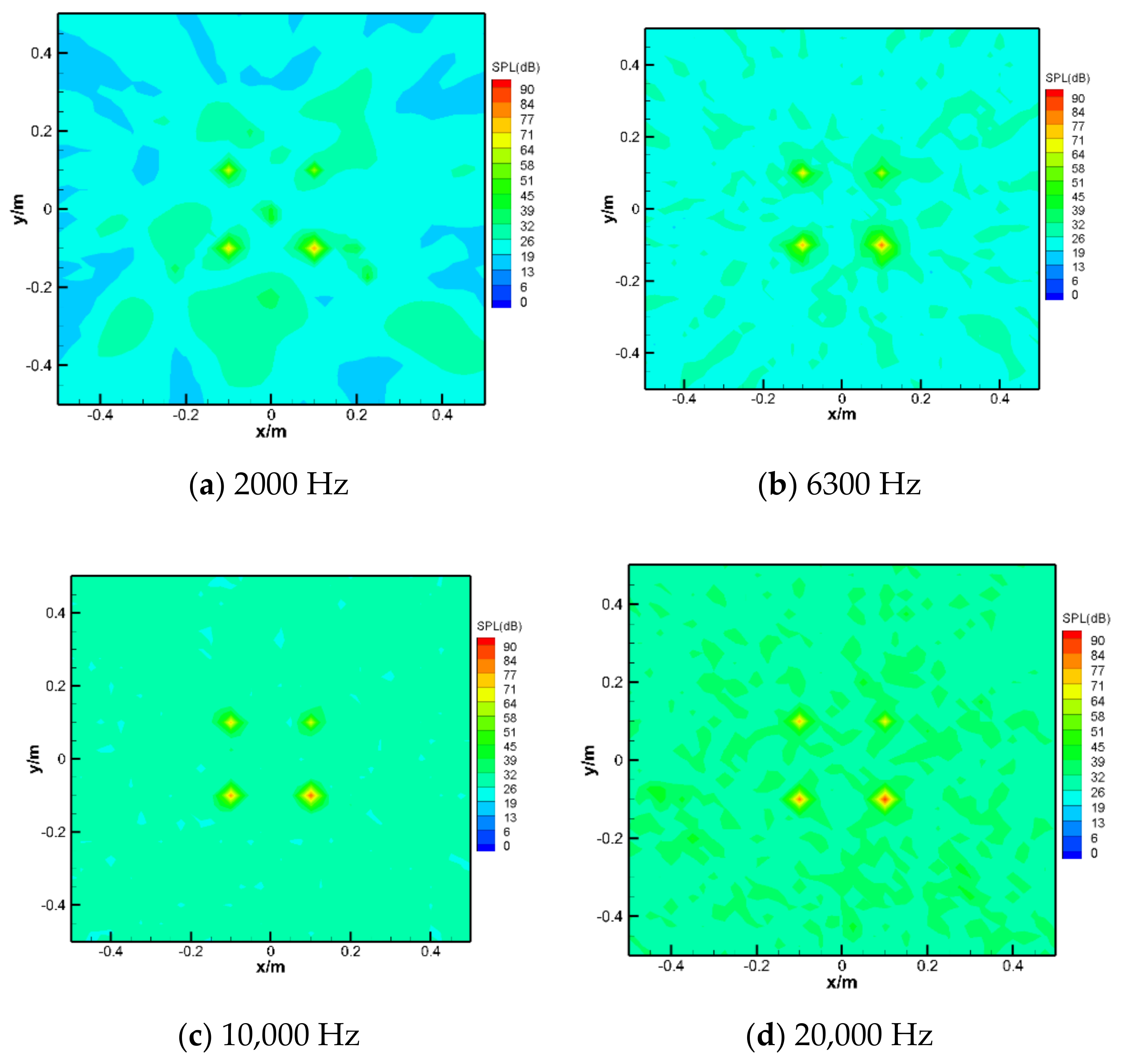
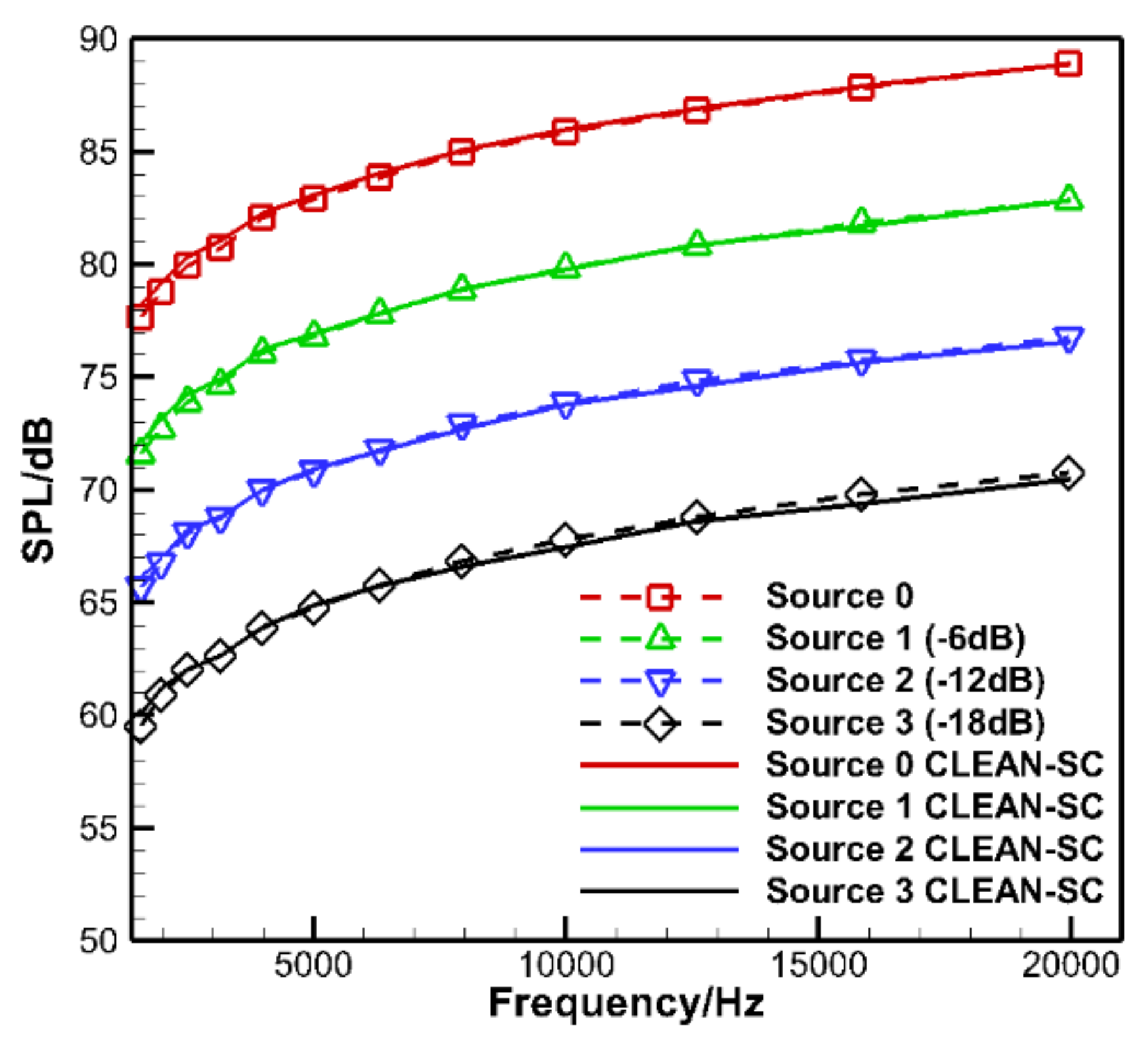
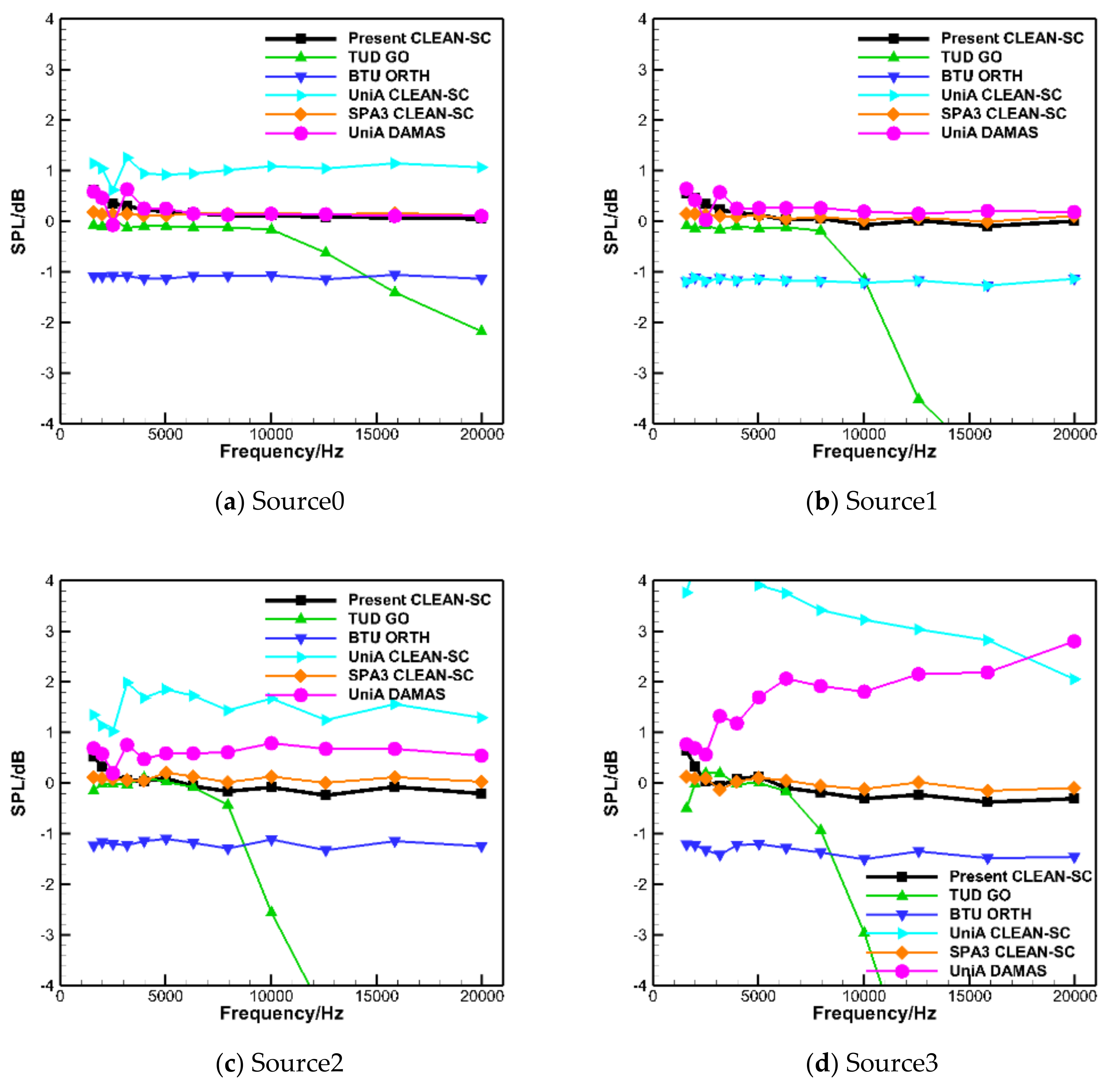
2.1. Results for Subcase A

Figure 2 shows the sound source distribution for different frequencies of the subcase A obtained by the present data processing method based on Clean-SC algorithm. It can be seen from Figure 2 that the program used in this paper can accurately identify the location of the noise source, and give a very clean image of the sound source.

Figure 3 shows the comparison between the identification results of four sound sources and the benchmark data for subcase A. The results show that the magnitudes of four sources are accurately identified using the present array data processing method with an error less than 0.5 dB.

Figure 4 shows the difference between the present results and benchmark data. For more extensive comparison, the results from other groups are also shown in the figure, including Brandenburg University of Technology Cottbus (BTU), University of Adelaide (UniA), PSA3, and Delft University of Technology (TUD) [37]. It can be seen from Figure 4 that the present array data processing method has a good accuracy in a wide frequency range with an error less than 0.5 dB. In the frequency range above 3000 Hz, the error is less than 0.2 dB. The results from other groups provide results generally within an error of 1 dB with two exceptions. The first one is the Orthogonal Beamforming (OB) method from BTU (BTU ORTH). The OB method assumes that the sources have different levels of intensity [39]. Therefore, it is expected that the OB method obtains relatively higher error with several equal sources. The other exception is the Global Optimization (GO) method [40] from TUD with the differential evolution as the optimization method. The underlying reason for the large error at higher frequencies might be due to the larger number of local optima. A different optimization method could be used to improve the results. In addition, the implementation details such as the stopping criterion for the iteration in Clean-SC and DAMAS, the different grid resolutions and the different steering vectors used can also contribute to the differences.

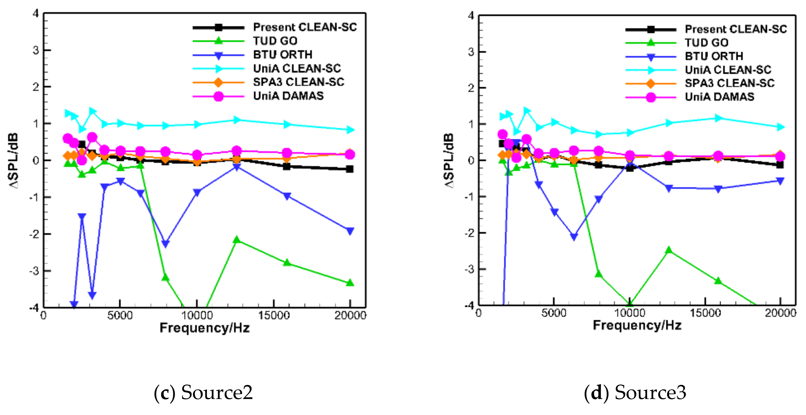
2.2. Results for Subcase B

Figure 5 shows the sound source distribution at different frequencies of the subcase B obtained by the present data processing program based on Clean-SC algorithm. It can be seen from Figure 5 that, even for the complex sound sources, the present program can accurately identify the location of the noise source, and get a clean image of the sound source for all the frequencies tested.

Figure 6 shows the comparison between the results of four sound sources and the benchmark data for subcase B. It can be observed from Figure 6 that, although the four sources differ in intensity by up to 18 dB (which means 63 times the energy difference), the magnitudes of four sound sources are accurately identified using the present array data processing software based on Clean-SC algorithm.

Figure 7 shows the difference between present identification results and benchmark data, along with the results from other researchers. Compared between Figure 4 and Figure 7, it can be seen that the accurate identification of non-equal intensity complex sound sources requires a higher-resolution algorithm, especially for the accurate identification of the weakest sound source (−18 dB). For the weakest Source3, only the array identification methods of PSA3 and the present paper can achieve high accuracy, for which the error above 3000 Hz is less than 0.2 dB. The error of the array identification method of UniA based on Clean-SC algorithm is within 1 dB in subcase A. However, in more complex subcase B, the calculation error increases significantly. For the weakest Source3, the error of the array identification method of UniA can reach 3 dB. The large error for the weak sources might be due to the implementation details of the different methods, which indicates that it is still a challenge for the evaluation of the weak sources in the presence of much stronger sources. This also shows that although the Clean-SC algorithm has been proposed for a long time, it still needs special attention to achieve its correct application, which fully verifies the importance of Sarradj’s work.

3. The Application of a Linear Array for the Identification of LE and TE Noise Source

3.1. Experimental Setup

The noise measurements are conducted in the low-speed open-jet wind tunnel in Northwestern Polytechnical University. The wind tunnel has a rectangular exit with dimensions of 0.3 m × 0.09 m. The maximum inflow velocity is 100 m/s with turbulence intensity below 1%. The uncertainty of the inlet mean velocity is within 0.5%. A NACA65(12)-10 blade with a chord of 150 mm and a span of 300 mm is employed as the baseline blade. The blade is fixed by two plexiglass side-plates, as shown in Figure 8a.

A linear array with 32 unequally spaced microphones is employed to identify and characterize the noise source of the blade. The array is 0.69 m below the airfoil with the array center located at the mid-chord of the blade. The microphones are installed on a hard-wall surface. The measured sound pressure levels (SPL) are assumed to be 6 dB larger than that of their actual values assuming a total reflecting. It must be noted that, in order to remove the background noise, the correction methods for the effects of reverberation and shear layer on sound propagation developed by our group [41] was used in this study. The 1/4 inch BSWA microphones are utilized in the experiment. All the microphones are calibrated by a standard noise source with a frequency of 1000 Hz and a SPL of 94 dB. The acoustic time signals are recorded with a sampling rate of 32,768 Hz for 10 s. The narrowband spectra are computed with a Hanning window of 50% overlap and a frequency resolution of 32 Hz. The so-called “BT product” is 320, where B is the frequency bandwidth and T is the sampling time. As a result, the autospectral random uncertainty is approximately ${\epsilon }_r=3.95\%$, which results in a random SPL uncertainty of $u_{r,\mathrm{SPL}}\in \left\{-0.18,0.17\right\}$ dB [42].

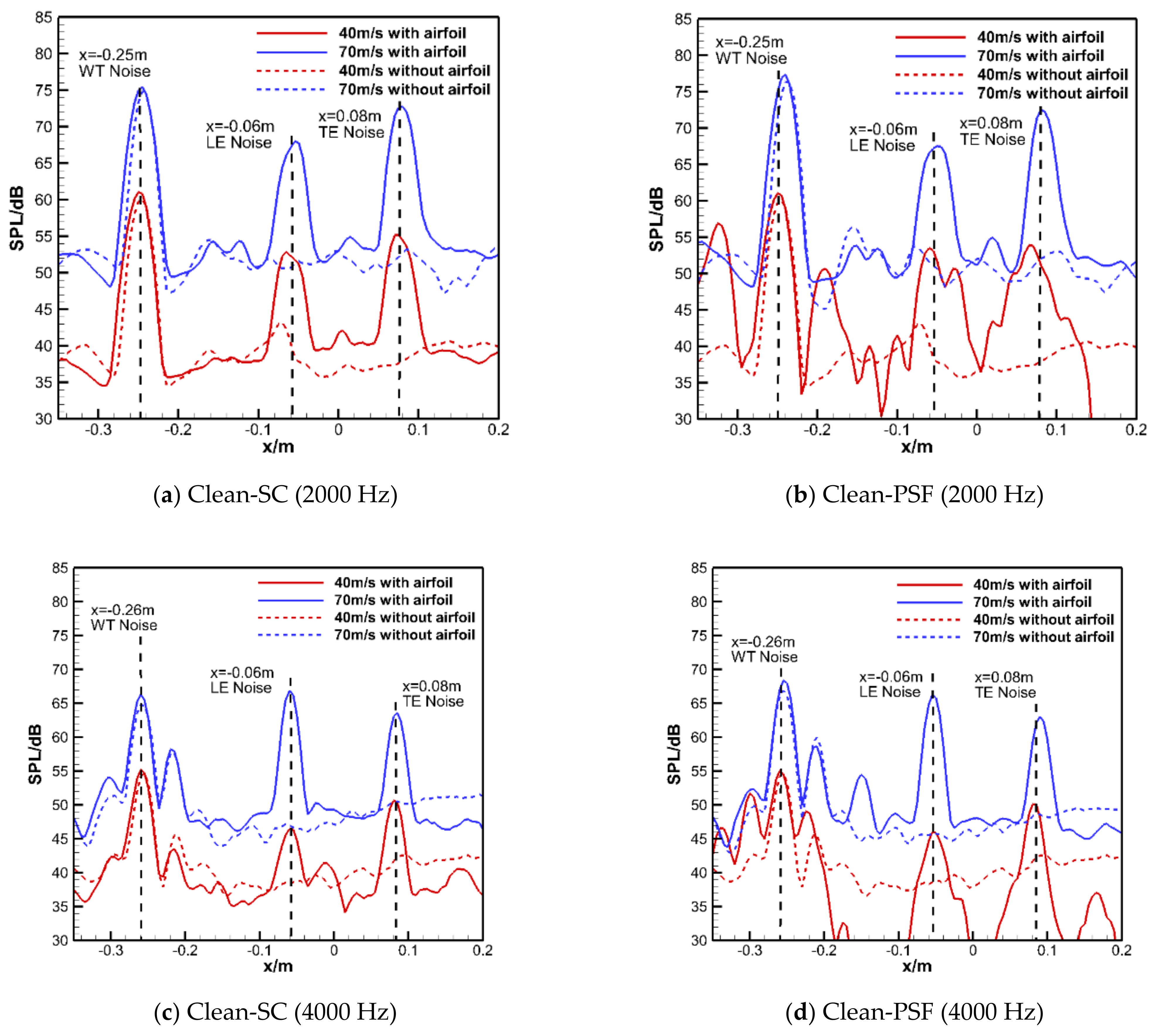
3.2. LE and TE Noise Sources Identification

The NACA65(12)-10 blade LE and TE noise are tested with various inflow velocities at an angle of attack of 0 degrees. The flow speeds are of 20~70 m/s, and the corresponding Reynolds numbers are 200,000~700,000. Figure 9a shows the beamforming results based on the Clean-SC method. It can be seen that very “clean” noise source identification is obtained with the present array method. The wind tunnel jet noise source (WT noise), and the LE and TE noise sources are all well identified. In addition, Clean-PSF algorithm was also employed to localize the LE and TE noise sources, and the results were compared with that from the Clean-SC algorithm. As shown in Figure 9b, the results obtained by the two algorithms are slightly different.

Figure 10 is a comparison of the sound source identification results between Clean-PSF algorithm and Clean-SC algorithm. It can be observed that the results with Clean-PSF algorithm have more side-lobes compared to that of the Clean-SC algorithm. There are two obvious side-lobes at x = −0.32 m and x = −0.18 m near the source of wind tunnel in the results with Clean-PSF algorithm. The side-lobes might be due to the fact that the jet noise is a distributed noise source. Further detailed comparison of Figure 10 shows that the noise level of the sound source identified by Clean-PSF algorithm is about 2 dB higher than that identified by Clean-SC algorithm.

4. Study of the TE Noise Reduction with Serrated Treatment Using Linear Microphone Array

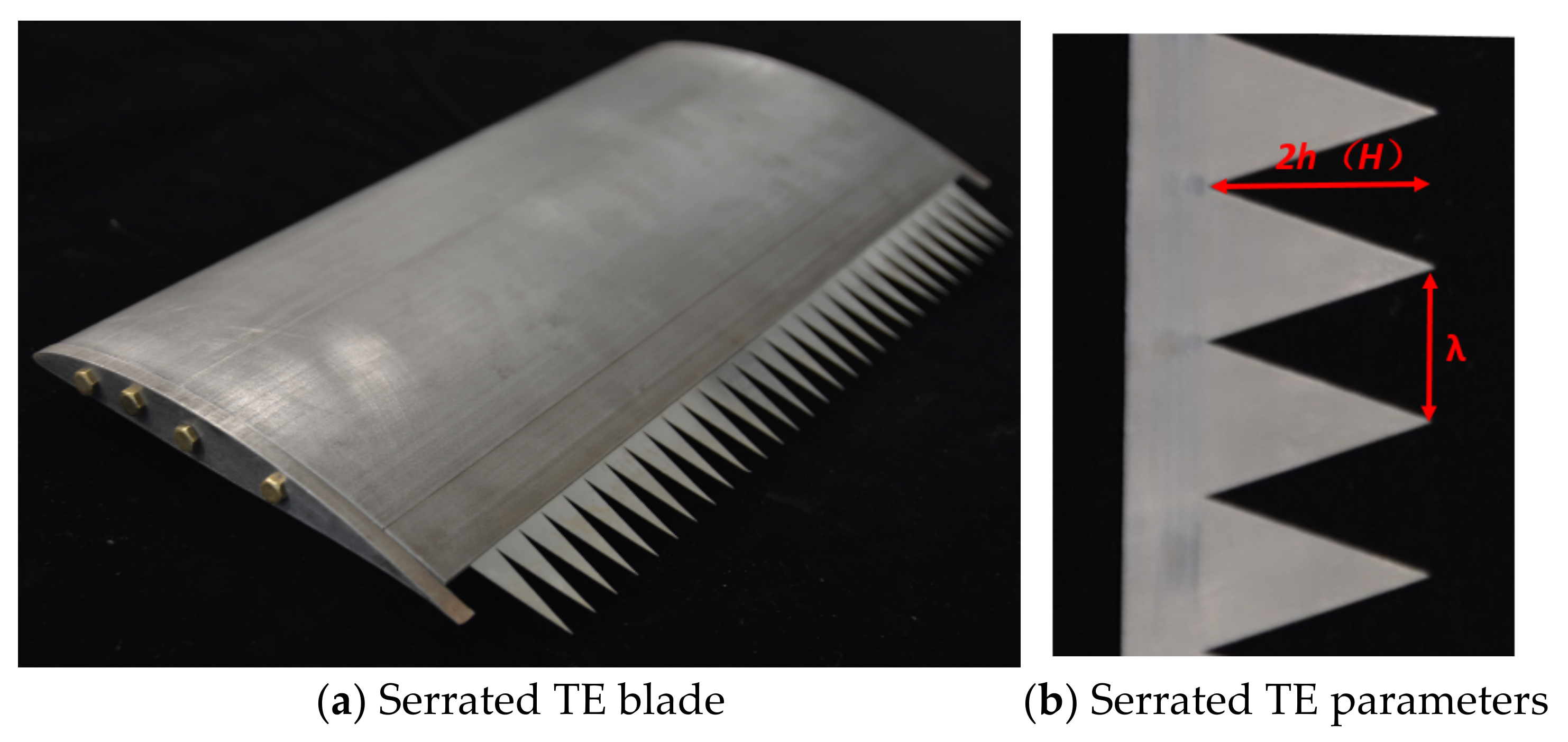
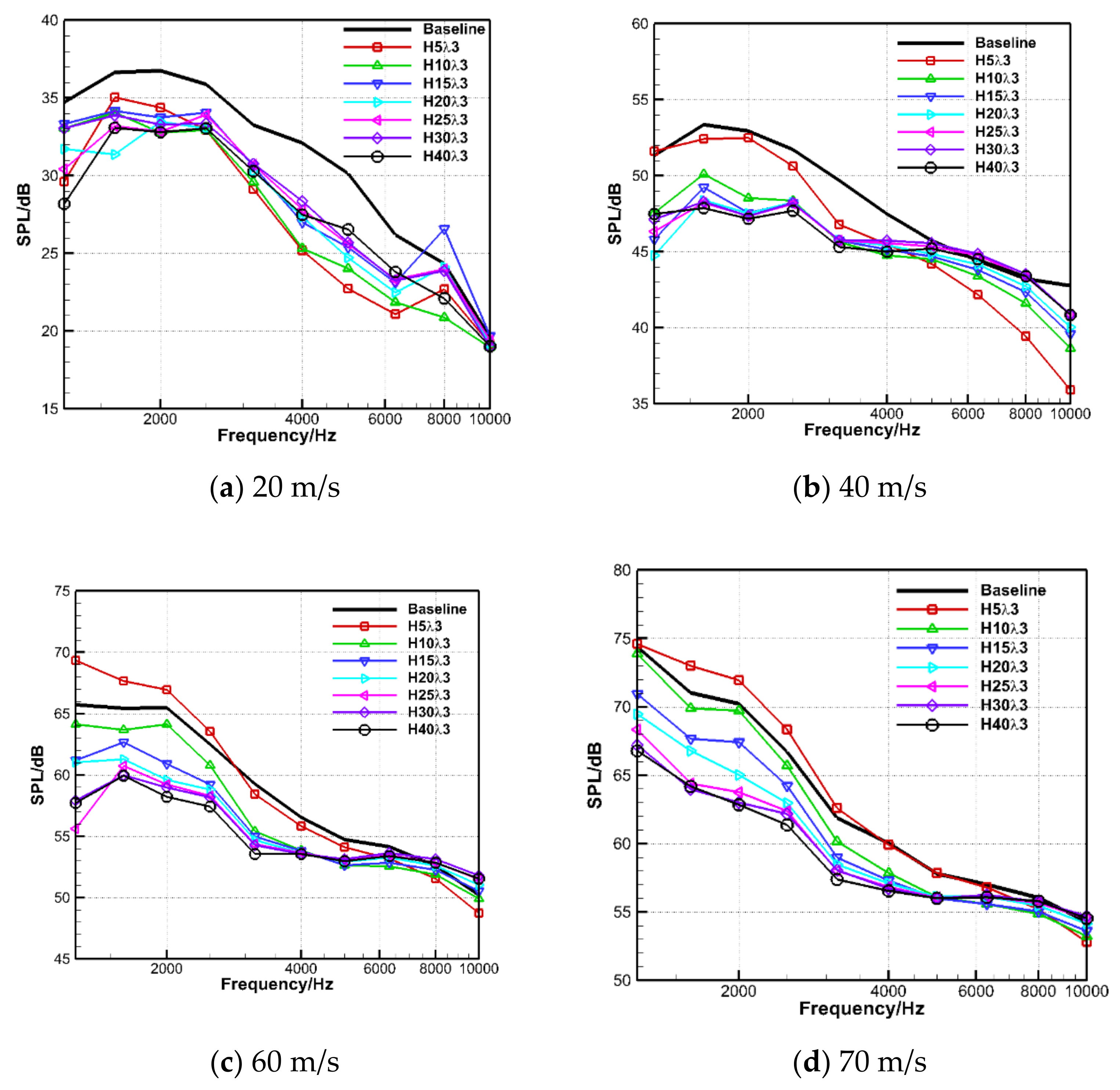
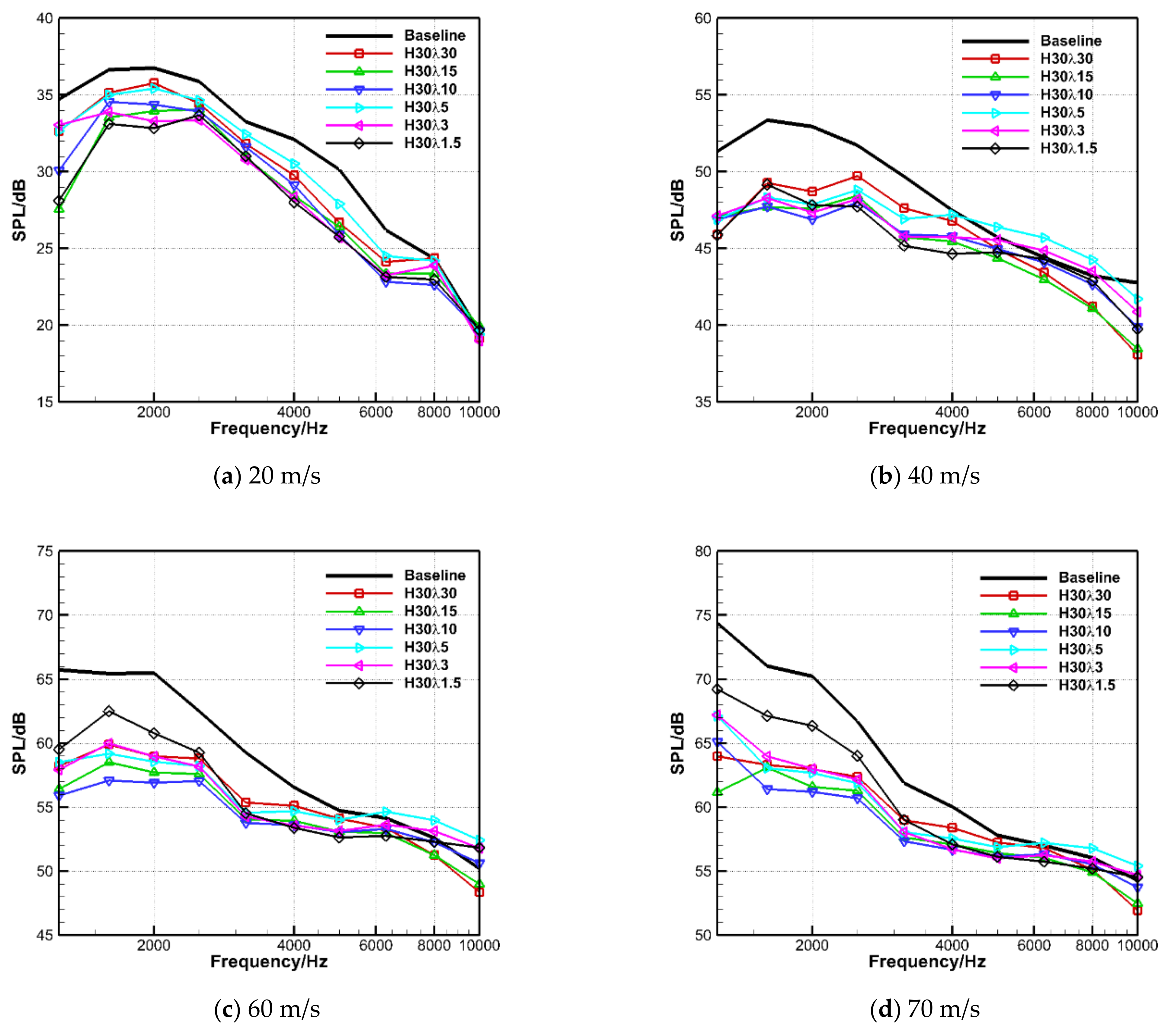
4.1. Serrated TE Configurations

The TE noise reduction with serrated treatments for NACA65(12)-10 blade was experimentally investigated using the same linear array. In order to systematically parameterize the noise reduction effect and regularity of the TE serration, a total of 12 different serrated blades, as shown in Figure 11a, were designed and tested in this experiment. Figure 11b shows the definitions of the sawtooth amplitude (2h) and wavelength (λ).

Table 1. Design parameters of the serrated TE configuration.

No.	Blade	$2\mathit{h} \left(\mathbf{mm}\right)$	$2\mathit{h}/\mathit{c}$	λ (mm)	$\mathit{\lambda }/\mathit{c}$	$\mathit{\lambda }/\mathit{h}$
0	Baseline	0	0	-	-	-
1	H5λ3	5	0.033	3	0.02	1.2
2	H10λ3	10	0.067	3	0.02	0.6
3	H15λ3	15	0.100	3	0.02	0.4
4	H20λ3	20	0.133	3	0.02	0.3
5	H25λ3	25	0.167	3	0.02	0.24
6	H30λ3	30	0.200	3	0.02	0.20
7	H40λ3	40	0.267	3	0.02	0.15
8	H30λ1.5	30	0.200	1.5	0.01	0.10
9	H30λ5	30	0.200	5	0.03	0.33
10	H30λ10	30	0.200	10	0.07	0.67
11	H30λ15	30	0.200	15	0.10	1.00
12	H30λ30	30	0.200	30	0.20	2.00

gives the design parameters of the serrated TE blades. In this table, c means the chord of the blade.

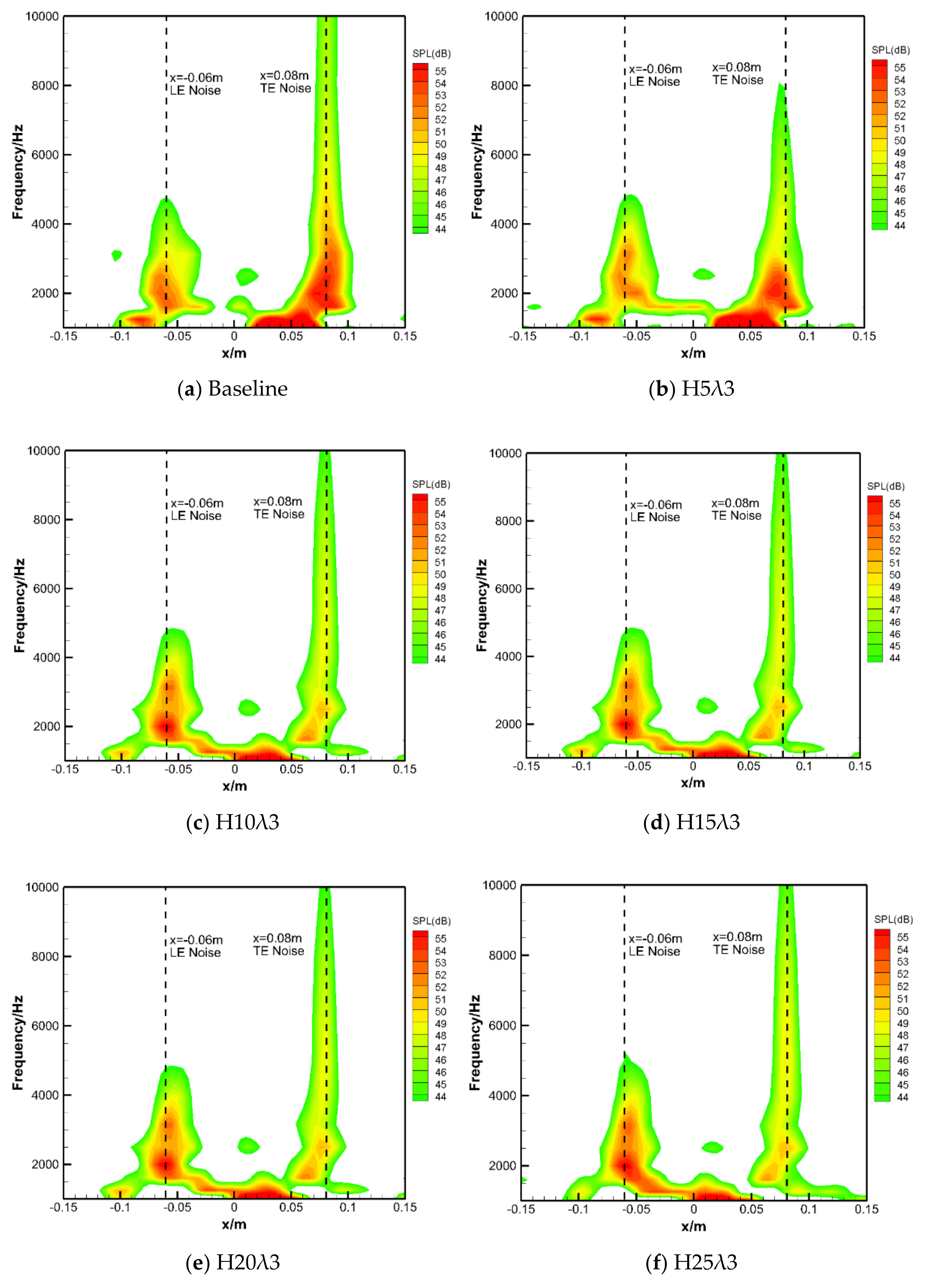
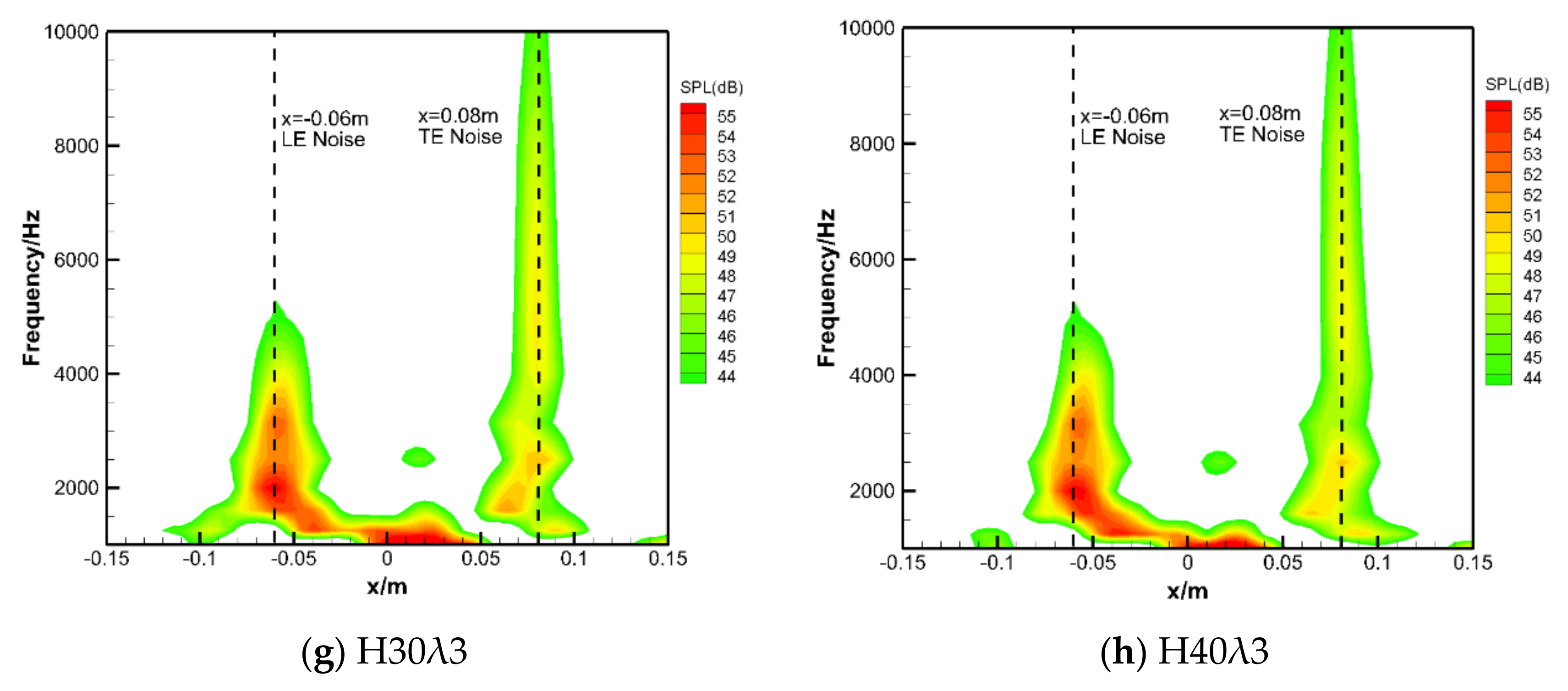
4.2. Results and Discussions

Firstly, the influence of the sawtooth amplitude on the TE noise characteristics is investigated. Figure 12 shows the sound source identification maps of different serration amplitudes under the flow condition of U = 40 m/s and with sawtooth wavelength λ = 3 mm. It can be seen from the figure that both the LE noise and TE noise sources can be separated correctly. The LE noise is barely affected by the serrated TE modification, while the TE noise can be significantly reduced with the serrated treatment. It can also be found from Figure 12b that the sawtooth H5λ3 has an obvious noise reduction effect for high-frequency noise.

It could be seen from the beamforming results that the main lobes of LE and TE noise all have some width in space. The magnitude of the LE and TE noise should be the sum of sound level in specified space. In this study, the sound pressure levels of LE and TE noise are evaluated using the following equation:

$$L_{LE}=10\cdot \lg \left(\frac{{\displaystyle \sum _{n=N_{\min }}^{N_{\max }}{10}^{0.1L_n}}}{N_{\max }-N_{\min }+1}\right)$$

(1)

where L_n is the sound pressure level at position n. Suppose that the LE and TE noise source center is at the position of maximum overall sound pressure level OASPL (in frequency band of 1000 to 10,000 Hz), N_min and N_max are, respectively, the upstream and downstream positions where the OASPL is 3 dB smaller than the maximum OASPL.

Figure 13 shows the 1/3 octave spectra of the TE noise for the blade possessing different sawtooth amplitudes and with the wavelength of 3 mm at airflow speeds of 20 m/s, 40 m/s, 60 m/s and 70 m/s. It can be seen from Figure 13 that the TE serrations can effectively reduce the TE noise. At flow speed of 20 m/s, the noise can be decreased by 4–5 dB below 8000 Hz for most of the serrated airfoils tested. However, the serrations have a negligible noise reduction effect for high frequency above 8000 Hz. Moreover, no obvious noise reduction law is obtained about the serration amplitude. When the airflow velocity is 40 m/s, except for the H5λ3 blade, the noise reduction effect of other serrated treatments has insignificant differences. The TE noise can be reduced by 3–7 dB below 5000 Hz. However, when the frequency is above 5000 Hz, the noise reduction effect is obviously weakened. With the increase in airflow velocity to 60 m/s and 70 m/s, the noise reduction difference between different sawtooth configurations increases. The low-frequency noise can even be enlarged by the H5λ3 blade. In general, the TE serrations can effectively reduce the low- to mid-frequency noise, while they might have a negligible noise reduction effect in the high-frequency range. The serrations with a larger amplitude generally obtain a higher noise reduction level.

Figure 14 shows the 1/3 octave spectra of the TE noise for the blades with different sawtooth wavelengths and with an amplitude of 30 mm. The inflow speeds are, respectively, 20 m/s, 40 m/s, 60 m/s and 70 m/s. It can be seen from Figure 14 that, at 20 m/s, the H30λ1.5 configuration has a large noise reduction in the frequency band of 1250~10,000 Hz, and the noise can be reduced by 3–4 dB. When the airflow velocity is 40 m/s, the TE serrations can considerably mitigate the TE noise below 4000 Hz. However, when the frequency is above 4000 Hz, the noise reduction effect is obviously weakened, and at some frequencies, the TE noise can be enlarged. With the increase in airflow velocity up to 60 m/s and 70 m/s, the noise reduction difference between different sawtooth treatments increases. The serration with the smallest wavelength H30λ1.5 has the smallest noise reduction, and the serration H30λ10 has the largest noise reduction. The maximum noise reduction effect can be up to 15 dB. Similar to the results in Figure 1, the serrations with various wavelengths can effectively reduce the low-frequency noise. However, the serrations have a negligible noise reduction effect for high frequencies or even increase the high-frequency noise. In addition, there is no obvious noise reduction law about the serration wavelength. From the above discussions, it can be concluded that the use of TE serrations for noise reduction is a very complicated issue. The noise reduction level is sensitive to both the serration amplitude and wavelength. Moreover, the noise reduction level changes a lot with the inflow conditions. The detailed acoustic database presented in this study is beneficial to develop noise prediction models for noise reduction with TE serrations [43,44,45], which will be our focus in the future study.

5. Conclusions

The source identification technology based on the Clean-SC algorithm was successfully used in this study to investigate the noise reduction effect of serrated TE treatment. Clear and quantitative sound radiation results from the TE noise source were obtained. According to this study, the conclusions are outlined below.

The current array data reduction program based on Clean-SC algorithm was assessed using Sarradj’s benchmark case. As indicated by Sarradj, although Clean-SC algorithm has been proposed for a long time, it still needs special attention to its correct application to achieve the best effect. The assessment results show that the present array data processing method has a good accuracy with an error less than 0.5 dB in a wide frequency range. The correct implementation of the Clean-SC algorithm is guaranteed for the study of noise reduction using TE serrations.

In the present study, it is found that the noise level of the sound source identified by the Clean-PSF algorithm is approximately 2 dB higher than that identified by the Clean-SC algorithm. This result shows the necessities to consider the interference effect of the sound sources on the identification results using phased microphone array.

The serrated TE treatments are found to be an effective noise reduction modification. The TE noise can be considerably reduced by the serrations with a maximum noise reduction effect up to 15 dB. However, the serrations can only achieve significant noise reduction effects in the low- to mid-frequency range, while they obtain negligible noise reduction effects in the high-frequency range or even increase the high-frequency noise. In addition, the noise reduction effect is sensitive to both the serration amplitude and wavelength. In general, the noise reduction effect increases with the serration amplitude, while no obvious noise reduction law is observed for the serration wavelength. Moreover, the noise reduction effect can be affected by the inflow conditions such as the incoming velocities. The results show that the use of TE serrations for noise reduction is a very complicated issue. To obtain the best noise reduction, the sawtooth configuration should be carefully designed according to the actual working conditions and airflow parameters.

References

1. Gliebe, P.R. Observations on Fan Rotor Broadband Noise Characteristics. In Proceedings of the 10th AIAA/CEAS Aeroacoustics Conference Proceedings, AIAA, Manchester, UK, 10–12 May 2004. [Google Scholar]
2. Curle, N. The influence of solid boundaries upon aerodynamic sound. Proc. R. Soc. London. Ser. A Math. Phys. Sci. 2006, 231, 505–514. [Google Scholar]
3. Williams, J.E.F.; Hall, L.H. Aerodynamic sound generation by turbulent flow in the vicinity of a scattering half plane. J. Fluid Mech. 1970, 40, 657. [Google Scholar] [CrossRef]
4. Crighton, D.G.; Leppington, F.G. Scattering of aerodynamic noise by a semi-infinite compliant plate. J. Fluid Mech. 1970, 43, 721–736. [Google Scholar] [CrossRef]
5. Crighton, D.G. Radiation from vortex filament motion near a half plane. J. Fluid Mech. 1972, 51, 357–362. [Google Scholar] [CrossRef]
6. Chandiramani, K.L. Diffraction of evanescent waves, with applications to aerodynamically scattered sound and radiation from unbaffled plates. J. Acoust. Soc. Am. 1974, 55, 19–29. [Google Scholar] [CrossRef]
7. Levine, H. Acoustical Diffraction Radiation. J. Acoust. Soc. Am. 1972, 52, 1092. [Google Scholar] [CrossRef]
8. Howe, M.S. The generation of sound by aerodynamic sources in an inhomogeneous steady flow. J. Fluid Mech. 1975, 67, 597–610. [Google Scholar] [CrossRef]
9. Howe, M.S. The influence of vortex shedding on the generation of sound by convected turbulence. J. Fluid Mech. 1976, 76, 711–740. [Google Scholar] [CrossRef]
10. Chase, D.M. Sound radiated by turbulent flow off a rigid half-plane as obtained from a wavevector spectrum of hydrodynamic pressure. J. Acoust. Soc. Am. 1972, 52, 1011–1023. [Google Scholar] [CrossRef]
11. Chase, D. Noise radiated from an edge in turbulent flow according to a model of hydrodynamic pressure—Comparison with a jet-flow experiment. In Proceedings of the 7th Fluid and PlasmaDynamics Conference, Palo Alto, CA, USA, 17–19 June 1974; pp. 1041–1047. [Google Scholar]
12. Davis, S.S. Theory of discrete vortex noise. AIAA J. 1975, 13, 375–380. [Google Scholar] [CrossRef]
13. Howe, M. A review of the theory of trailing edge noise. J. Sound Vib. 1978, 61, 437–465. [Google Scholar] [CrossRef]
14. Marcolini, M.; Brooks, T.; Pope, D. Airfoil Self-Noise and Prediction; NASA RP-1218; NASA: Washington, DC, USA, 1989. [Google Scholar]
15. Brooks, T.; Hodgson, T. Trailing edge noise prediction from measured surface pressures. J. Sound Vib. 1981, 78, 69–117. [Google Scholar] [CrossRef]
16. Amiet, R. Noise due to turbulent flow past a trailing edge. J. Sound Vib. 1976, 47, 387–393. [Google Scholar] [CrossRef]
17. Amiet, R. A note on edge noise theories. J. Sound Vib. 1981, 78, 485–488. [Google Scholar] [CrossRef]
18. Howe, M. Trailing edge noise at low mach numbers. J. Sound Vib. 1999, 225, 211–238. [Google Scholar] [CrossRef]
19. Adams, H. Patent Application for a “Noiseless Device”. No. US2071012A, 22 February 1937. [Google Scholar]
20. Graham, R. The silent flight of owls. Roy. Aero. Soc. J. 1934, 286, 837–843. [Google Scholar] [CrossRef]
21. Lilley, G.M. A study of the silent flight of the owl. In Proceedings of the 4th AIAA/CEAS Aeroacoustics Conference, No.1998-2340, AIAA, Toulouse, France, 2–4 June 1998. [Google Scholar]
22. Bohn, A. Edge noise attenuation by porous edge extensions. In Proceedings of the 14th AIAA Aerospace Sciences Meeting, No. 76-80, Washington, DC, USA, 26–28 January 1976. [Google Scholar]
23. Khorrami, M.; Choudhari, M. Application of Passive Porous Treatment to Slat Trailing Edge Noise; NASA TM-212416; NASA: Washington, DC, USA, 2003. [Google Scholar]
24. Sarradj, E.; Geyer, T. Noise generation by porous airfoils. In Proceedings of the 13th AIAA/CEAS Aeroacoustics Conference, No. 2007-3719, Rome, Italy, 21–23 May 2007. [Google Scholar]
25. Finez, A.; Jondeau, E.; Roger, M.; Jacob, M. Broadband noise reduction with trailingedge brushes. In Proceedings of the 16th AIAA/CEAS Aeroacoustics Conference Proceedings, No. 2010-3980, Stockholm, Sweden, 7–9 June 2010. [Google Scholar]
26. Howe, M.S. Aerodynamic noise of a serrated trailing edge. J. Fluid Struct. 1991, 5, 3–45. [Google Scholar] [CrossRef]
27. Howe, M.S. Noise produced by a sawtooth trailing edge. J. Acoust. Soc. Am. 1991, 90, 482–487. [Google Scholar] [CrossRef]
28. Oerlemans, S.; Fisher, M.; Maeder, T.; Kogler, K. Reduction of wind turbine noise using optimized airfoils and trailing-edge serrations. NLR-TP-2009-401. AIAA J. 2009, 47, 1470–1481. [Google Scholar] [CrossRef]
29. Gruber, M.; Joseph, P.F.; Chong, T.P. Experimental Investigation of Airfoil Self Noise and Turbulent Wake Reduction by the Use of Trailing Edge Serrations. In Proceedings of the 16th AIAA/CEAS Aeroacoustics Conference, No. 2010-3803, Stockholm, Sweden, 7–9 June 2010. [Google Scholar]
30. Liang, J. Experimental and Numerical Study on Mechanism and Suppression Method of Turbo-Machinery Broadband Noise. Ph.D. Thesis, Northwestern Polytechnical University, Xi’an, China, 2016. [Google Scholar]
31. Michel, U. History of acoustic beamforming. In Proceedings of the Berlin Beamforming Conference (BeBeC), Berlin, Germany, 21–22 November2006. [Google Scholar]
32. Venkatesh, S.R.; Polak, D.R.; Narayanan, S. Beamforming algorithm for distributed source localization and its application to jet noise. AIAA J. 2003, 41, 1238–1246. [Google Scholar] [CrossRef]
33. Lowis, C.; Joseph, P. A focused beamformer technique for separating rotor and stator-based broadband sources. In Proceedings of the 12th AIAA/CEAS Aeroacoustics Conference, No. 2006-2710, Cambridge, CA, USA, 8–10 May 2006. [Google Scholar]
34. Brooks, T.F.; Humphreys, W.M. A deconvolution approach for the mapping of acoustic sources (DAMAS) determined from phased microphone arrays. J. Sound Vib. 2006, 294, 856–879. [Google Scholar] [CrossRef] [Green Version]
35. Brooks, T.F.; Humphreys, W.M.; Plassman, G.E. DAMAS processing for a phased array study in the NASA Langley jet noise laboratory. In Proceedings of the 16th AIAA/CEAS Aeroacoustics Conference, No. 2010-3780, Stockholm, Sweden, 7–9 June 2010. [Google Scholar]
36. Sijtsma, P. CLEAN Based on Spatial Source Coherence. Int. J. Aeroacoustics 2007, 6, 357–374. [Google Scholar] [CrossRef]
37. Sarradj, E.; Herold, G.; Sijtsma, P.; Martinez, R.M.; Geyer, T.F.; Bahr, C.J.; Porteous, R.; Moreau, D.; Doolan, C.J. A microphone array method benchmarking exercise using synthesized input data. In Proceedings of the 23rd Aiaa/ceas Aeroacoustics Conference, Aiaa Aviation Forum, Denver, CO, USA, 5–9 June 2017. [Google Scholar]
38. Hogbom, J.A. Aperture synthesis with a non-regular distribution of interferometer baselines. Astron. Astrophys. Suppl. 1974, 15, 417–426. [Google Scholar]
39. Sarradj, E. A fast signal subspace approach for the determination of absolute levels from phased microphone array measurements. J. Sound Vib. 2010, 329, 1553–1569. [Google Scholar] [CrossRef]
40. Aalgoezar, A.; Snellen, M.; Martinez, R.; Simons, D.G.; Sijtsma, P. On the use of global optimization methods for acoustic source mapping. J. Acoust. Soc. Am. 2017, 141, 453–465. [Google Scholar] [CrossRef]
41. Qiao, W.Y.; Ji, L.; Tong, F.; Wang, L.F.; Chen, W.J. Separation and Quantification of Airfoil Le- and Te-Noise Source with Microphone Array. In Proceedings of the 2018 Berlin Beamforming Conference, BeBeC2018 D-14, Berlin, Germany, 5–8 March 2018. [Google Scholar]
42. Bendat, J.S.; Piersol, A.G. Random Data: Analysis and Measurement Procedures, 4th ed.; John Wiley & Sons: Hoboken, NJ, USA, 2010. [Google Scholar]
43. Loiodice, S.; Drikakis, D.; Kokkalis, A. An efficient algorithm for the retarded time equation for noise from rotating sources. J. Sound Vib. 2018, 412, 336–348. [Google Scholar] [CrossRef] [Green Version]
44. Loiodice, S.; Drikakis, D.; Kokkalis, A. Emission surfaces and noise prediction from rotating sources. J. Sound Vib. 2018, 429, 245–264. [Google Scholar] [CrossRef]
45. Ritos, K.; Drikakis, D.; Kokkinakis, I.W. Wall-pressure spectra models for supersonic and hypersonic turbulent boundary layers. J. Sound Vib. 2019, 443, 90–108. [Google Scholar] [CrossRef] [Green Version]
Figure 1. Layout of the planar array with sixty-four microphones.
Applsci 11 00572 g001
Figure 2. Sound source distribution for subcase A at different frequencies.
Applsci 11 00572 g002
Figure 3. Comparison between the present results and the benchmark case for subcase A.
Applsci 11 00572 g003
Figure 4. Comparison of the present results with other studies for subcase A.
Applsci 11 00572 g004aApplsci 11 00572 g004b
Figure 5. Sound source distribution for subcase B at different frequencies.
Applsci 11 00572 g005
Figure 6. Comparison between the present results and the benchmark case for subcase B.
Applsci 11 00572 g006
Figure 7. Comparison of the present results with other studies for subcase B.
Applsci 11 00572 g007
Figure 8. Microphone array and the test setup.
Applsci 11 00572 g008
Figure 9. Noise maps of the blade test for U = 40 m/s.
Applsci 11 00572 g009
Figure 10. Comparison of the sound source identification results between Clean-PSF algorithm and Clean-SC algorithm.
Applsci 11 00572 g010
Figure 11. The serrated trailing-edge (TE) blade and parameter definitions.
Applsci 11 00572 g011
Figure 12. The sound source distribution of the blade with different sawtooth amplitudes (U = 40 m/s).
Applsci 11 00572 g012aApplsci 11 00572 g012b
Figure 13. Spectra of the TE noise with different sawtooth amplitudes (λ = 3 mm).
Applsci 11 00572 g013
Figure 14. Spectra of the TE noise with different sawtooth wavelengths (H = 30 mm).
Applsci 11 00572 g014