Improving the Strategy of Maintaining Offshore Wind Turbines through Petri Net Modelling


Department of Aeronautical and Automotive Engineering, Loughborough University, Loughborough, Leicestershire LE11 3TU, UK
*
Author to whom correspondence should be addressed.
Appl. Sci. 2021, 11(2), 574; https://0-doi-org.brum.beds.ac.uk/10.3390/app11020574
Submission received: 6 December 2020
/
Revised: 31 December 2020
/
Accepted: 6 January 2021
/
Published: 8 January 2021
(This article belongs to the Special Issue Wind Power Technologies)
Abstract
:In order to improve the operation and maintenance (O&M) of offshore wind turbines, a new Petri net (PN)-based offshore wind turbine maintenance model is developed in this paper to simulate the O&M activities in an offshore wind farm. With the aid of the PN model developed, three new potential wind turbine maintenance strategies are studied. They are (1) carrying out periodic maintenance of the wind turbine components at different frequencies according to their specific reliability features; (2) conducting a full inspection of the entire wind turbine system following a major repair; and (3) equipping the wind turbine with a condition monitoring system (CMS) that has powerful fault detection capability. From the research results, it is found that periodic maintenance is essential, but in order to ensure that the turbine is operated economically, this maintenance needs to be carried out at an optimal frequency. Conducting a full inspection of the entire wind turbine system following a major repair enables efficient utilisation of the maintenance resources. If periodic maintenance is performed infrequently, this measure leads to less unexpected shutdowns, lower downtime, and lower maintenance costs. It has been shown that to install the wind turbine with a CMS is helpful to relieve the burden of periodic maintenance. Moreover, the higher the quality of the CMS, the more the downtime and maintenance costs can be reduced. However, the cost of the CMS needs to be considered, as a high cost may make the operation of the offshore wind turbine uneconomical.
1. Introduction
Wind power is one of the fastest-growing emerging industries in recent years. For example, 205 GW of wind power capacity has been built in Europe to date, accounting for 15% of the EU’s total electricity demand in 2019 [1]. Nowadays, although most wind turbines are on land, an increasing number of wind turbines are being deployed offshore due to better wind resources, less visual impact, and less noise pollution and land use issues at offshore sites [2]. However, the current high operation and maintenance (O&M) costs of offshore wind turbines (OWTs) are challenging the sustainable development of the offshore wind industry [3]. Therefore, how to reduce the O&M costs of OWTs, thereby lowering the cost of offshore wind power, has become an urgent issue that needs to be addressed.
The maintenance of OWTs is affected by many factors, such as component reliability, site accessibility, weather conditions, maintenance strategies, availability of spare parts, vessels, tools, maintenance crews, etc. Hence, it is essential to carefully schedule a maintenance plan beforehand. To help the operators schedule an optimal maintenance plan, much effort has been made by scholars in recent years. For example, Nilsson and Bertling investigated the influences of different maintenance strategies and demonstrated the positive contribution of the condition monitoring systems (CMSs) to cost reduction [4]. McMillan and Ault compared scheduled maintenance and condition-based maintenance using Markov chains [5]. Dao et al. investigated the impact of reliability on the O&M costs of OWTs [6].
The factors that have a direct impact on the O&M costs of offshore wind farms have also been investigated. Scheu et al. investigated the impact of the accuracy of the weather forecast, maintenance strategies, and maintenance fleet on the availability of offshore wind farms [7]. Besnard et al. developed a model to optimise the maintenance of offshore wind farms with the consideration of the number of maintenance personnel, the types of maintenance vessels, the use of a helicopter for site access, and the location of accommodation [8]. Sperstad considered whether the maintenance vessels should be purchased or chartered based on the site locations and also discussed the influences of wave height and vessel fleet size on the maintenance process [9]. Dalgic et al. studied the impact of multiple environmental factors on the maintenance costs of offshore wind farms [10]. In their research, four different transportation systems with different speeds, access restrictions, costs, and carrying capabilities were considered. Much research has been conducted for reducing the O&M costs of offshore wind farms. For example, Eecen et al. developed a mathematical tool to help the operators better estimate the O&M costs of offshore wind farms [11]. Abdollahzadeh et al. used a multi-objective particle swarm optimisation method to optimise the opportunistic maintenance strategy of a wind farm [12]. Tuyet and Chou also proposed an approach to optimise the maintenance schedules for an OWT [13], which considered individual wind turbine components and grouped those based on their failure patterns. A more detailed review of the existing research on modelling the maintenance activities of OWTs can be found in [14]. The outcomes of these studies have provided strong support for decision-making during the operation of offshore wind farms.
However, although corrective maintenance and preventive maintenance strategies are used in combination in the maintenance practice of offshore wind farms, discrepancies still exist between the mathematical models developed and actual maintenance activities and many basic questions related to the O&M of OWTs have not been fully answered. As mentioned in [14], one of the main reasons for this is the lack of a more advanced mathematical modelling method to accurately describe the relevant maintenance activities. To meet this need, a new simulation model of OWT maintenance is developed using Petri nets (PNs) in this paper. The reason for choosing to use PNs is that, in contrast to conventional Discrete Event Simulation (DES) models, the PN model provides an intuitive graphical representation of a system of interest and it has been proven to be more flexible and computationally efficient, especially when modelling complex systems [15,16,17]. Recently, the PN has also demonstrated success in simulating the degradation and maintenance of wind turbines [18,19]. Hence, it is adopted in this study to simulate the following three new potential O&M measures, which have been identified from the literature review as important are studied:
Measure (1)—Carry out periodic maintenance of different wind turbine components at different frequencies according to their specific reliability features. The study of this measure will determine how often periodic maintenance should be conducted. Different wind turbine components develop faults at different periods. However, this phenomenon has not been taken into account in both current maintenance practice and the available mathematical maintenance models. To use maintenance resources (e.g., the size of the maintenance team, different kinds of vessels, service time, etc.) more efficiently and minimise unnecessary investigations, two levels of services, i.e., “basic service” and “advanced service”, are designed in the new PN model. The two levels of services are applied to different wind turbine components according to their reliability features. In the model, “basic service” refers to the checking and fixing of issues that may often occur but are difficult to monitor and may accelerate the degradation of key wind turbine components if are not fixed, such as the looseness of bolts, insufficient lubrication, etc. The key turbine components, such as main bearing, pitch bearings, gears, blades, generator, converter, tower structure, etc., will not be inspected during the period of “basic service”. By contrast, “advanced service” requiring more expensive maintenance resources will involve more tasks than “basic service”. In addition to the work that will be conducted during “basic service”, the key wind turbine components will be inspected during “advanced service” to find those faults that are not detected by the CMS. Almost all OWTs in operation are equipped with CMS to detect incipient faults occurring in key components and prevent the sudden failure of them [20]. Once one or more faults are detected, the corresponding maintenance will be arranged and conducted. Herein, it should be noted that unless the OWT is hit by external extreme events, the faults detected in the OWT assemblies (or subsystems) are usually repairable. In the modelling process of this paper, it is assumed that after the defective subsystems are repaired, their functions will be fully restored. In addition, it should be noted that in existing maintenance models, it is assumed that all minor faults can be fixed in one time of visit [5,14]. This is inconsistent with current industrial practice because the minor faults to be repaired are not known before the visit, so it is not known whether these minor faults can be repaired during the current visit. This discrepancy has been reduced in the new PN model developed in this paper, which allows an inspection and reporting of any minor faults first and then scheduled maintenance that takes dedicated actions to repair all the detected minor faults. Therefore, the PN model developed can more accurately describe the practical maintenance process of OWTs than previous studies.
Measure (2)—Conduct a full inspection of the entire wind turbine system following a major repair (i.e., the recovery from failure). Studying this measure will enable the utilisation of maintenance resources more effectively. A major repair is often associated with high costs due to the replacement of those defective components that cannot be repaired and the involvement of a range of maintenance resources, such as a large crane vessel that has powerful lifting capability, a large team to deliver the major repair, etc. Since so many maintenance resources are already in use it is wise to take the opportunity to conduct a full inspection of the wind turbine once the major repair is completed. To investigate the impact of such an approach upon the safety and reliability of the turbine system, in the PN model developed a full inspection of the entire wind turbine system is conducted following performing a major repair. Such an approach would benefit wind farms in the long run as they could run at the lowest cost. Since the relevant cost would be covered in the contract for performing the major repair, it will not be considered separately in the PN model developed. However, it is worth noting that this measure will affect the health state of the wind turbine components in the model.
Measure (3)—Equip the wind turbine with a CMS that has a more powerful fault detection capability. The study of this measure will investigate the impact of the application and quality of the CMS on the O&M of the OWT. Today, CMSs have been widely accepted as a valid tool to aid the O&M of OWTs [20,21,22]. Therefore, most of the existing maintenance models have considered them. However, a diversity of wind turbine CMSs has currently been developed. They are different in hardware cost and fault detection capability. Such differences are not taken into account in the existing models, resulting in inaccurate prediction results. This issue has been overcome by the new PN model developed in this paper.
The remaining part of the paper is organised as follows. In Section 2, an OWT composed of six critical subsystems is defined; In Section 3, the PN-based modelling technique is briefly reviewed; In Section 4, four types of PN models are developed for describing the maintenance activities in offshore wind farms; In Section 5, the downtime and maintenance costs in different scenarios are calculated using the PN models developed and the obtained results are discussed; In Section 6, the paper concludes with key research findings.
2. Structure, Health States, and Maintenance Strategies of the Offshore Wind Turbine
2.1. Structure of the OWT
To facilitate mathematical modelling, the structure, health states, and maintenance strategies of the OWT are defined in this section based on [18,19,23,24]. Due to the fact that gear-driven wind turbines currently have a large market share, a gear-driven OWT composed of six subsystems is considered. The six subsystems are the rotor system, main bearing system, drivetrain system, braking system, power system, and turbine structures, respectively.
- The rotor system is composed of the blades and the hub;
- The main bearing system provides safe support to the rotor system and enables rotation to occur with minimal friction;
- The drivetrain system consists of the main shaft and a gearbox that is also called accelerator;
- The braking system locks the wind turbine position in non-operational mode; for example, when the maintenance of the wind turbine is in progress or the wind turbine is shut down under extreme weather conditions. The braking system is also used to slow down the rotor when the wind speed is beyond cut-out speed, i.e., a protective shutdown of the turbine is required when wind speed exceeds cut-out speed of 25 m/s [10,12];
- The power system consists of a generator, a converter, and a transformer;
- The turbine structures include a nacelle, tower, and foundation.
Since the failure of these subsystems will lead to the shutdown of the turbine, their reliability will have a direct impact on the O&M of the OWT. For simplicity, the health state of these subsystems is classified into three categories in this study, i.e., healthy, fault, and failure. When the subsystems are in a healthy state, they will operate normally. When a minor fault is detected from a subsystem by the CMS, it is assumed that the subsystem is still able to work with the minor fault, but more care should be taken to monitor the development of the fault. This is the fault state. When the minor fault develops into a failure and is detected by the CMS, the wind turbine will be shut down immediately to prevent causing secondary damage or catastrophic consequence. For example, the broken blade may hit the tower, causing the entire wind turbine to collapse; the failure of the braking system may catch fire and lead to the burning of the entire nacelle of the wind turbine, etc. [25].
2.2. Maintenance Strategy
To reduce the downtime and the maintenance costs of the OWT, as considered in the existing maintenance models, three different maintenance strategies [26], i.e., corrective maintenance, periodic maintenance, and condition-based maintenance, are adopted. However, in this work they are further refined by considering the three new measures outlined in Section 1. The periodic maintenance will be delivered via two levels of services, namely, “basic service” and “advanced service”. Since “basic service” is essential in keeping the turbine operating at high efficiency in the long term and preventing the acceleration of the degradation of wind turbine components, in the new PN model it will be conducted every six months and will last for one day per turbine per instance [5,18]. Since the issues found in “basic service” are usually minor problems, in the PN model developed it is assumed that all of these will be fixed in one visit. By contrast, the “advanced service” will extend the activities to inspect the key wind turbine components. In this study, the period between the “advanced service” ranges from 3 months to 5 years in order to investigate the influence of this time interval on the downtime and maintenance costs of the OWT. The time required for carrying out “advanced service” is usually longer than the time for “basic service”. For simplicity, “advanced service” is assumed to last for two days per turbine per instance in the model. To further increase the safety and reliability of the wind turbine and utilise the maintenance resources more effectively, a full inspection is arranged following a major repair. Finally, considering that condition-based maintenance is highly dependent on the fault detection capability of the CMS, the influence of the fault detection capability of the CMS on the downtime and maintenance costs are also investigated in the paper. To the best of the authors’ knowledge, similar research has not been completed previously.
3. A Brief Review of Petri Net-Based Modelling Technology
To facilitate understanding of the PN models developed in this paper, the basics of the PN modelling method are briefly reviewed below. As shown in Figure 1, the bipartite graph of a PN model consists of four basic types of symbols, i.e., circles, rectangles, arrows, and tokens. The circles represent places, which are conditions or states of the system, such as component failure. In this paper, coloured patterns are used in order to differentiate between different places. The condition place, marked with yellow-horizontal-lines in the model, means that the model will perform predefined actions if the conditions in the place are met. The place filled by red-vertical-lines means that the simulation will be ended if a token is placed in it. Rectangles represent the transitions, which define the actions or events that cause the change in condition or state. It should be noted that when the time for completing the transition is zero, the rectangle is filled black. Otherwise, it will be blank. Arcs in the figure are used to set up the connections between places and transitions. To enhance the functions of the arcs, a slash and a number, n, next to the slash are used to represent a combination of n single arcs. In this case, it is said that the arc has weight n. When the weight is one, the slash will be absent from the arc for simplicity. In the PN models, small solid black circles are used to represent tokens in the places, which carry the information in the PNs. The dashed arcs mean the link between the connected places and transitions are conditional. The tokens will move via transitions once the enabling condition is satisfied, which offers the unique dynamic properties of the PNs. The transition will be enabled when the number of tokens contained in every input place is equal to, or greater than, the corresponding weight of the arc. The arc with a small solid circle on one end is known as inhibitor arc, which only links places to transitions. If the number of tokens in the place connecting the inhibitor arc is greater than or equal to the arc weight, the transition on the other end of the arc cannot fire even if the transition is already enabled. The marking of a PN, given by the position of the tokens in the net, at any particular time gives the instantaneous state of the system being modelled.
To ease understanding, Figure 2 shows an example of the PN model, in which the movement of tokens in the places occurs after a delay, illustrating a transition through the net. In the figure, the net has two input places and one output place connected by a timed transition indicated by a blank rectangle with a time delay t. There are two tokens in each input place. The two input places are connected by arcs of weight 1 and weight 2. The output place is connected by an arc of weight 1. As shown in the net on the left of the figure, the transition is enabled, hence after the delay of time t associated with the transition, the number of tokens indicated by the arc weights will be removed from the input places and placed in the output place. By following the rules outlined above, one token is taken out of the top input place and two from the lower and one token is placed in the output place as shown in the net on the right of the figure.
4. Dynamic PN Modelling of the O&M of an Offshore Wind Turbine
To simulate the O&M of an OWT, the following four PN models will be developed in this section:
- Operation Petri net (OPN)—for simulating the normal operation and periodic maintenance of an OWT. In the OPN, the design life of the turbine and the interval of the periodic maintenance will be defined.
- System Petri net (SPN)—for simulating the degradation, the health state of the turbine subsystems over time, and the shutdown of the turbine due to failure.
- Detection Petri net (DPN)—for simulating fault detection by the CMS.
- Recovery and Maintenance Petri net (RMPN)—for simulating the process to prepare and conduct the maintenance when a subsystem fails, or a subsystem fault is detected by the CMS.
The above four PNs communicate with each other and work synchronously as shown in Figure 3. After the design life of the OWT and the time interval of periodic maintenance are defined in the OPN, the natural degradation of the turbine subsystems will be simulated first by the SPN. The SPN results for individual subsystems will be fed into the DPN and RMPN. The fault detection results derived from the DPN, the information of the failure causing the shutdown of the turbine derived from the SPN, and the fault revealed during the “advanced services” derived from the OPN, will be fed into the RMPN. Then, based on the information received from the SPN and DPN, the RMPN will simulate the appropriate maintenance actions corresponding to the types of the faults and failure and their severities and consequences. Finally, the information derived from the RMPN will be used to update the corresponding information in the SPN. The simulation calculations of all PN models will be terminated when the design life of the wind turbine is reached.
4.1. Operation Petri Net (OPN)
As shown in Figure 4, the OPN is developed to simulate the normal operation and periodic maintenance of an OWT.
In the figure, the PN on the top governs the normal operation of the wind turbine within the design life. Transition “S1” indicates the design life of the wind turbine, which is set to be 30 years in this study. Once Transition “S1” fires, a token will be produced in Place “End of design life”, indicating the completion of the life of the wind turbine. Then, the instant transition, “S2”, is enabled, thereby firing immediately and a token will be produced in Place “End of one simulation”, and the simulation will be terminated.
The PNs at the bottom, labelled “periodic maintenance” and “weather condition”, are used to simulate the periodic maintenance of the wind turbine. As mentioned earlier, the periodic maintenance in this study includes two levels of services. The “basic service”, BS for short in the figure for simplification, is for checking and fixing non-major issues; the “advanced service”, AS for short, is for checking the key wind turbine components and finding the faults not detected by the CMS. The two levels of the services are conducted at different frequencies according to the reliability features of individual components. Once one or more faults are detected during “advanced service”, maintenance will be planned and conducted to fix the faults. Due to the “advanced service” inspecting key wind turbine components, more maintenance resources (e.g., a bigger maintenance team, a larger vessel, longer service time, etc.) are required than for “basic service”. In the OPN, the firing times of Transitions “PM1” and “PM3” are the time intervals of the two levels of services. A token produced in Places “BS starts” and “AS starts” means that periodic service is about to begin. A token in Place “need inspection” determines that a full inspection of the turbine should be conducted. The firing times of Transitions “PM2” and “PM5” are assumed to be one day and two days, respectively, indicating the duration of “basic service” and “advanced service” of each turbine every time. It should be noted that the turbine will be stopped during maintenance.
In addition, as maintenance is not allowed in bad weather, Transitions “PM2” and “PM5” are inhibited if a token is in Place “Bad weather”. In the existing maintenance models, the time taken waiting for favourable weather to enable maintenance to take place is usually represented by a mathematical function of sea conditions and the maximum wave height and wind speed that the maintenance is allowed to be conducted in [18,19]. In the current study, for simplicity, Transitions “C1” and “C2” are designed to describe the alternation between good and bad weather. The delay time due to weather conditions is governed by a Weibull distribution function. The Weibull distribution function for C1 is characterised by β = 3.2 and η = 42 days; and the Weibull distribution function for C2 is characterised by β = 3.2 and η = 7 days, respectively. Here, β and η are the shape factor and the scale parameter of the distribution. These values of β and η can be easily modified based on the actual environmental situation in the offshore wind farm. Once Transitions "PM2" or "PM5" fire, a token will be produced in Place “BS completed” or “AS completed”, respectively, which indicates the completion of the periodic maintenance. If a token is produced in Place “AS completed”, the RMPN will be embedded into the model for preparing and conducting the maintenance if any fault was detected during the periodic maintenance. Finally, the token produced will be removed from either Place “BS completed” or Place “AS completed”.
4.2. System Petri Net (SPN)
As shown in Figure 5, the SPN is developed to simulate the degradation and the health state of the wind turbine subsystems over time, and the shutdown of the turbine due to failure.
In the model, the natural degradation of the subsystems is indicated by three health states, namely “Normal operation”, “Subsystem fault”, and “Subsystem failure”. The subsystems will initially operate normally without any fault, indicated by a token in Place “Normal operation” for each subsystem. Due to natural degradation, the subsystems may develop a fault, exhibiting abnormal features such as increased vibration and temperature, decreased efficiency, etc. In this case, the health state of the affected subsystem/subsystems will be marked as “Subsystem fault”. The degradation time from “normal” to “fault” is indicated by Transitions “W1” to “W6”. Once a token is produced in any of the condition places “Subsystem fault”, the DPN will be embedded into the model to simulate the fault detection by the CMS as required by the predefined condition. Once a subsystem fault is successfully detected by the CMS, the RMPN will be embedded into the model.
However, if the subsystem fault was not detected by the CMS, the fault may continue to develop and eventually lead to the failure of the subsystem. The failure of the subsystem will cause the shutdown of the wind turbine. To enable simulation of the continual development of the fault, the predefined conditions, which embedding DPN into the model, will be removed from the corresponding places representing the subsystem faults and then these places will become normal places. The process of the undetected faults eventually leading to the shutdown of the turbine is modelled by Transitions “W7” to “W12”. In the study, it is assumed that the times for Transitions “W1” to “W12” satisfy Weibull distributions characterised by the parameters listed in Table 1. In the table, the data has been estimated based on the wind turbine failure rate data published in the open literature [18,19]. In [19], the scale parameters η in the distributions for computing the times from normal to fault and failure are estimated based on the assumption that the time spans in the two scenarios will cover 80% and 20% of the Mean Time to Failure (MTTF) respectively of the corresponding subsystems. The MTTF is the inverse of the failure rate listed in Table 1. The shape parameters β in the distributions are assumed to be larger than 1 for all six subsystems in order to describe the increasing deterioration of the subsystems over time. In the model, it is assumed that the wind turbine will be shut down immediately as soon as any one of the six subsystems fails. This is modelled by Transitions “W13” to “W18”. Once a token is produced in any one of Places “Subsystem failure”, the wind turbine will be shut down and the RMPN will be embedded into the model.
Once the failed subsystem is recovered, which will be modelled in the RMPN, a token will be passed to Place “Wind turbine recovered”, and Transition “W19” will be activated hence starting the full inspection of the entire wind turbine system. Once any fault is detected (i.e., if there is a token in any one of Places “Subsystem fault”), the RMPN will be embedded into the model again.
4.3. Detection Petri Net (DPN)
Since the DPN is developed for simulating the fault detection process by the CMS, the DPN is embedded into the model only when there is at least one fault occurring in any one of the six subsystems.
As Figure 6 shows, in the DPN, Transition “D1” governs the whole process. The arcs, represented by the dashed arrow lines, connect Transition “D1” with the condition places, “Fault is detected” and “Fault is not detected”. The probabilities that a token transfers to either of the two places are dependent on the fault detection capability of the CMS. This fault detection capability may be affected by many factors, such as the types of the sensors, condition monitoring algorithm, the scope of components that the CMS monitors, etc. [27]. In this study, to investigate the influence of the quality of the CMS on the O&M, three scenarios are considered. These scenarios are “Without using CMS”, “After using a basic CMS”, and “After using a premier CMS”. The probabilities that the faults can be detected by the CMS in the three scenarios are listed in Table 2. The probability data for the scenario of using a basic CMS is from [28]. The probability data for the scenario of using a premier CMS is set to be 0.997 for all six subsystems in order to investigate the maximum contribution of the CMS to the O&M under ideal conditions. All the data in Table 2 can be modified based on the actual capability of the CMS. Once the fault is detected by the CMS, i.e., a token is produced in Place “Fault is detected”, the RMPN will then be embedded into the model to prepare the essential maintenance resources and then fix the fault. If the fault is not detected by the CMS, a token is produced in Place “Fault is not detected” and no action will be taken in the DPN. Once a token is produced either in Place “Fault is detected” or in Place “Fault is not detected”, the DPN will be removed from the model. The undetected fault will continue to develop with time. This developed fault will either eventually lead to the failure of the corresponding subsystem or it will be discovered during the next run of the inspection during “advanced service”.
4.4. Recovery and Maintenance Petri Net (RMPN)
The RMPN is developed for simulating the process of preparing and conducting the maintenance when any subsystem fails, or a subsystem fault is detected by the CMS or revealed during an “advanced service”. As shown in Figure 7, once a subsystem failure occurs or a subsystem fault is detected by the CMS, a repair request will be made immediately via Transition “M1”. Then, the maintenance team will be informed, and a meeting will be arranged for planning the maintenance. In the study, it is assumed that 12 h, indicated by Transition “M2”, are needed to perform these activities. It is also assumed in this study that another 12 h, denoted by Transition “M3”, are required for planning and approving the maintenance. The preparation for the maintenance is started by producing a token in both Places “Charter vessel” and “Organise crews, tools and spare parts”. It is assumed that 10 to 30 days, denoted by Transition “M4”, are required for checking weather conditions, identifying maintenance window, and chartering the appropriate maintenance vessel, and 7 to 14 days, denoted by Transition “M5”, are required for organising maintenance crews, collecting maintenance tools and preparing spare parts. Both of the transition times of “M4” and “M5” are assumed to follow a normal distribution. As soon as both maintenance vessel and maintenance crews, tools, and spare parts are available, a token will be produced in Place “Travel to site” via Transition “M6”. The sea transportation time is assumed to be 3 h and indicated by Transition “M7” in this study. In reality, it depends on the offshore distance of the wind farm and the cruise speed of the vessel and can be easily varied in the model. Upon arrival at the site, some preparations need to be undertaken (e.g., navigate the position of the vessel and lift the platform of a Jack-up vessel out of the water surface). This will take about 2 to 4 h depending on the situation. This preparation time is denoted by Transition “M8”. Then, the maintenance will be conducted. The maintenance time, indicated by Transition “M9”, is assumed one day for repairing all faults or seven days for recovering the subsystem from the failure. This transition time can be adapted for the offshore wind farm being considered at the time using available practical data. It is worth noting that the wind turbine should remain stopped and not allowed to be started during the entire maintenance period. Finally, a token will be produced in Place “Maintenance completed” and the RMPN will be removed from the model when the maintenance is completed. The new health state of the corresponding subsystem will be fed back to the SPN. The token in the corresponding place, “Subsystem failure” or “Subsystem fault”, will be removed and a token will be passed to corresponding Place “Normal operation” in the SPN.
It is worth noting that all parameters used in the models developed above are only for facilitating model development. Although they are extracted from open literature, they should be updated in the practical application based on the concrete situation of the OWT of interest. In real life, the values of these model parameters are dependent on many factors. This is why a significant discrepancy was observed in the survey [6]. For instance, the offshore distance of the OWT will affect its accessibility and transportation costs. The concept, size, and the location of the OWT (that may affect wind speed and turbulence) in the offshore wind farm will affect its failure rate, thereby influencing its availability and maintenance costs. Moreover, the same type of OWT made by the same supplier may show different reliability and efficiency performances when they are deployed in different offshore wind farms because of the differences in marine and offshore conditions. For these reasons, the model parameters should be updated according to the actual situation of the OWT in practical applications.
5. Simulation Results and Discussions
A new OWT maintenance model is developed in this Section by assembling the above four types of PN models based on the following assumptions:
- The CMS has no hardware reliability issues;
- The subsystem faults and failure caused by natural disasters (e.g., earthquakes, tsunamis, etc.) are not considered;
- All detected faults are repairable, and all failures can be recovered through maintenance;
- The health state of a subsystem after maintenance is regarded as good as new.
Then, based on the data listed in Table 1 and Table 2, the simulation calculation is carried out by using the following steps:
Step 1: Define the parameters of the PNs:
- Initialise the places and transitions, and the arcs between them, as well as the conditions for the condition places and the terminate places;
- Import the fixed transitions times and compute the variable ones (e.g., time to failure, time for chartering a vessel, etc.) by randomly sampling with the corresponding distributions as in [29];
- Define the conditional probability of any conditional arcs.
Step 2: Identify and fire the enabled transition that has the minimum switching time in the complete model;
Step 3: Recompute the times of any transitions that are still enabled;
Step 4: Repeat Steps 2 and 3 until a token is produced in one of the condition places or terminate places;
Step 5: Activate the conditions predefined for the condition places or terminate place containing a token;
Step 6: If a token is produced in a terminate place, the present iteration will be ended. Otherwise, repeat Steps 2 to 5.
Step 7: Iterate the above simulation until the predefined iteration time is reached.
To validate the convergence of the model, the average number of drivetrain failures within the lifetime of the OWT is calculated. The calculation results obtained when the time intervals of “basic service” and “advanced service” are six months and one year respectively are shown in Figure 8.
From Figure 8, it is seen that after the simulation starts, the calculation result of the average number of drivetrain failures fluctuates at the beginning. Then, it becomes stable gradually with the increasing number of simulations and finally converges to a stable value after the number of simulations is over 50,000. In the following calculations, to ensure the reliability of the calculation results, 100,000 simulations will be performed to predict the target parameters.
5.1. System and Subsystem Analysis
When the wind turbine is equipped with a basic CMS and only “advanced service” is assumed to be conducted every six months, the average number of failures and the average number of faults occurring in each subsystem in the lifetime of the turbine can be obtained by calculating the average value of the times that each subsystem fails and the average value of the times that each subsystem develops a fault in the lifetime of the turbine in 100,000 simulations. The calculation results are listed in Table 3.
From Table 3, it is found that despite different subsystems showing different reliability features, the total number of subsystem failures causing the shutdown of the turbine within the whole design life of the turbine is only 0.68. The fact that there are so few failures is attributed to the use of the CMS and frequent inspections as well as the immediate action to repair the faults as soon as they are detected.
From the simulation results, it is also found that the total downtime of the turbine is 162.23 days, which means the availability of 98.52% in its lifetime if neglecting the influence of extreme events. Such high availability is very satisfactory for an OWT, but it could be further improved by some approaches; for example, optimising the time interval of periodic maintenance, using a higher quality CMS, etc. However, it is well known that frequently carrying out inspection and using a higher quality CMS will increase costs. How to make a trade-off between the availability and the O&M costs becomes a difficult question that operators of all wind farms must consider. To answer this question, further research has been conducted and described below.
5.2. Impact of Maintenance Strategy
The influence of the maintenance strategy on the O&M of the OWT is investigated in the following sections. In the calculations, corrective maintenance, condition-based maintenance, and full inspection following the recovery of the subsystem from failure are all adopted. In order to keep the wind turbine operating at high efficiency in the long term and prevent the accelerated degradation of the wind turbine components, the “basic service” is assumed to be carried out every six months in the simulation. The time interval of the “advanced service” is assumed to be a variable, ranging from 3 months to 5 years. Herein, it is worth noting that “basic service” is conducted only when its time interval is shorter than the time interval of the “advanced service”.
5.2.1. The Influence of the Time Interval of “Advanced Service”
When the time interval of “advanced service” is three months, four months, six months, one year, two years, three years, four years, and five years, the average number of faults detected by the CMS and found in the full inspections and the average number of failures causing the shutdown of the wind turbine are calculated. The corresponding calculation results are shown in Figure 9.
From Figure 9, it is seen that with the increase of the time between “advanced service”, the average number of faults detected by the CMS and found in the full inspections decreases gradually. This implies that the wind turbine will have more chances to run with a fault or faults. However, this does not necessarily mean an increased availability of the turbine, because “running with a fault or faults” will increase the probability of subsystem failure and thereby increased number of unexpected shutdowns of the turbine, as indicated by the increasing tendency of the average number of failures in Figure 9. The unexpected shutdown due to subsystem failure is often associated with a long downtime, especially in offshore wind farms.
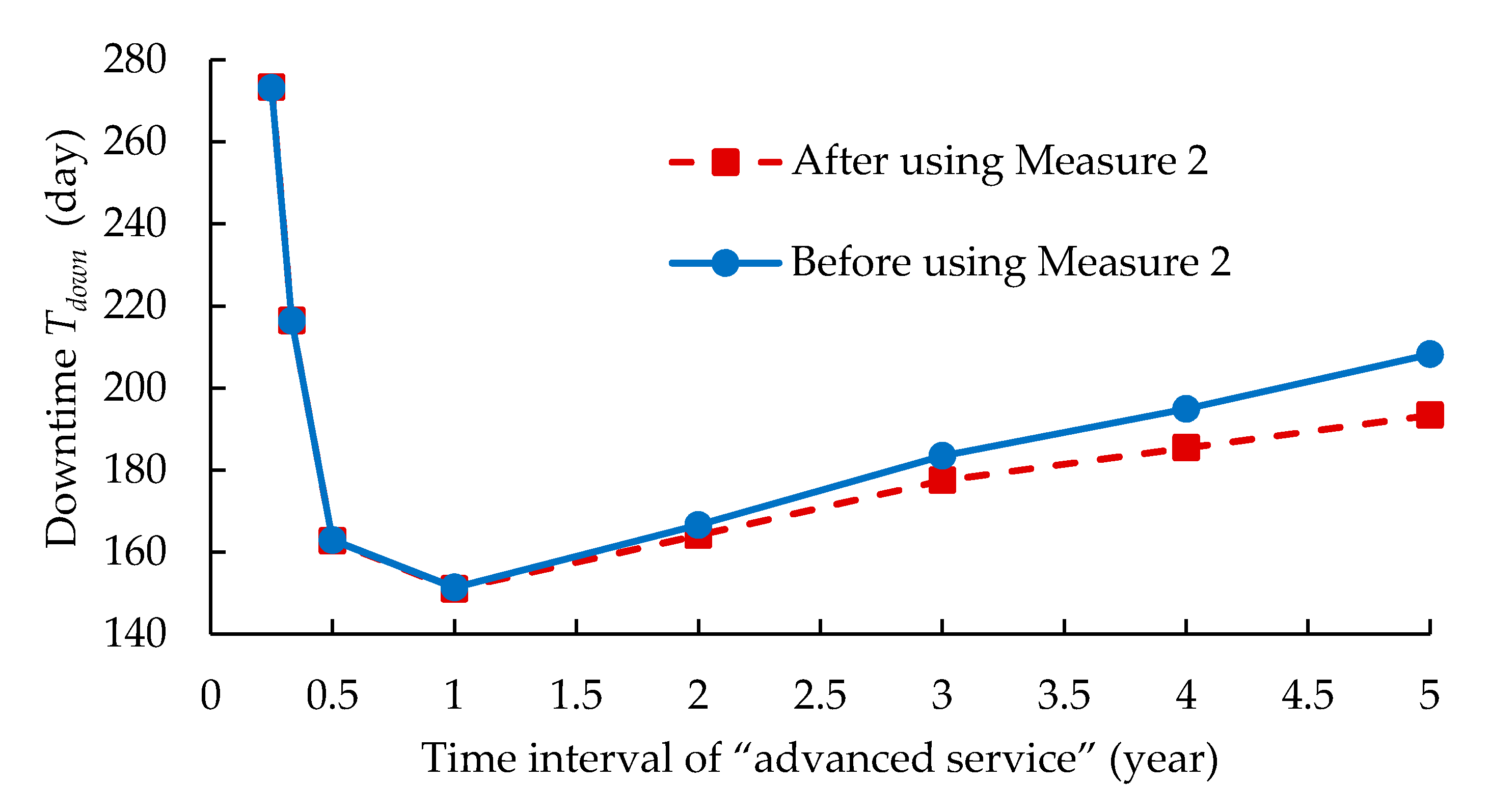
To understand the trade-off between the availability and maintenance costs, the downtime and the maintenance cost caused by the faults and failures in Figure 9 are calculated using the PN model developed. To demonstrate the benefit of taking Measure (2) proposed in Section 1, the downtime and maintenance costs before using the new measure are also calculated for comparison. The results of downtime obtained before and after taking Measure (2) are shown in Figure 10.
From Figure 10, it is found that
- With the increase of the time between the “advanced service” maintenance, the downtime of the turbine caused by the subsystem faults and failures decreases first and then increases after the time interval is greater than one year. This means that although “advanced service” is beneficial in decreasing the chance of subsystem failure and the consequent shutdown of the turbine, too frequent “advanced service” is not good either because it may cause a waste of time on unnecessary inspections. On the other hand, too infrequent “advanced service” may result in more unexpected shutdowns of the turbine due to the increased number of subsystem failures (see Figure 9);
- The minimum downtime is observed when the time between “advanced service” is one year regardless of whether Measure (2) is taken. So, from the perspective of downtime, 1 year is the optimal time interval for carrying out “advanced service”;
- The longer the time between “advanced service” maintenance, the more benefits of using Measure (2) are observed. This proves the positive contribution of Measure (2) to the availability of the wind turbine.
However, the contribution of Measure (2) to the economy of the wind farm is not only dependent on its contribution to downtime reduction but is also dependent on its contribution to maintenance costs. Therefore, the maintenance costs before and after taking this measure are also calculated. In the calculation, both the costs of corrective maintenance and periodic maintenance are taken into account. The cost of corrective maintenance is dependent on the subsystem in which the fault occurs, fault severity, consequence (i.e., whether causing a subsystem failure), and the expense of the maintenance vessels. In this paper, two different types of vessels are used for different purposes. The first type of vessel is crew transfer vessel, which is used to transfer maintenance crews to the site to check and repair faults; the second type of vessel is a crane vessel, which is used to recover the failed subsystems. Therefore, the maintenance cost, , is calculated by
where NI is the number of “advanced services” performed, is the average cost of each “advanced service”, is the number of “basic services” performed, is the average cost of each “basic service”. and are the average cost for repairing a fault in subsystem and the average cost for recovering the subsystem from failure respectively. They are listed in Table 4.
Likewise, and are the average number of faults occurring in subsystem and the average number of failures of subsystem during the lifetime of the wind turbine respectively. and are the charter rates of a typical crane vessel and a typical crew transfer vessel respectively. and are the number of days that the two types of vessels will be chartered every time. These values about the maintenance vessels are deduced based on [18,19,30]. Then, the maintenance costs in different scenarios are calculated using Equation (1), and the results are shown in Figure 11.
From Figure 11, it is found that
- After taking the proposed Measure (2), the resultant red dash line is clearly below the blue solid line if the time interval of “advanced service” is longer than one year. This proves the positive contribution of the new measure to the reduction of maintenance costs if the “advanced service” is conducted infrequently;
- As for the downtime shown in Figure 10, maintenance costs initially decrease and then increase with the increase of the time interval of “advanced service”. However, Figure 11 shows that the minimum maintenance costs occur when the time interval of “advanced service” is 0.5 years, indicating that 0.5 years is the optimal time interval from the perspective of maintenance cost. This contradicts the optimal time interval obtained from the perspective of downtime in Figure 10.
Then, which time interval is the optimal one? To answer this question, a new maintenance strategy assessment criterion, namely Cost for achieving turbine availability per day, is proposed. It is denoted by and calculated by
where refers to the design life of the wind turbine. This represents the cost of keeping the turbine running per day. Assume the design life of the turbine is 30 years and there are 365.25 days per year, then days. represents the total downtime of the wind turbine in its lifetime.
Then, is calculated based on the data of in Figure 10 and in Figure 11. The calculation results are shown in Figure 12. From the figure, it is found that shows a similar variation tendency to the maintenance cost in Figure 11, regardless of whether Measure (2) is used. In other words, with the increase of the time between "advanced service" maintenance, it initially decreases until the time interval reaches 0.5 years, and then increases as the time interval increases. This suggests that six months is the optimal time between “advanced service” maintenance for achieving the economical operation of the OWT. Finally, the figure once again shows the economic benefit of adopting Measure (2) with the impact becoming significant once the time between “advanced service” maintenance is longer than one year.
5.2.2. Condition-Based Maintenance
The impact of the application and quality of the CMS on the O&M of an OWT is also investigated. Three scenarios are considered in the investigation although due to the structure of the model developed other scenarios could easily be considered. They are
- Scenario 1—CMS not used, only use “advanced service” every half year;
- Scenario 2—Use a basic CMS and “advanced service” takes place every half year;
- Scenario 3—Only use a premier CMS that has a powerful fault detection capability as described in Table 2 without adopting “advanced service”.
The number of faults repaired, the number of failures recovered, the downtime, and maintenance costs are calculated. All results are listed in Table 5 for comparison.
From Table 5, it is seen that
- When using a CMS, a greater number of faults are detected and repaired. Moreover, the better the quality of the CMS, the more faults will be detected and repaired.
- The comparison of the data obtained in Scenario 1 and Scenario 2 suggests that the unexpected shutdown of the wind turbine can be significantly prevented by using a basic CMS, conducting a frequent inspection, and taking prompt action to repair the faults. Thanks to the use of the basic CMS, the consequent downtime and maintenance cost are significantly reduced;
- The comparison of the results in Scenario 3 and Scenario 2 shows that when the fault detection capability of the CMS is improved, the number of failures, downtime and maintenance costs can be further reduced.
The data obtained in Scenario 3 suggests that periodic maintenance will become unnecessary when using a premier CMS. However, this is based on the assumption that the fault detection capability of the CMS is 0.997. Undoubtedly, it is impossible to achieve such a well-performing CMS in reality at the moment, but it does suggest that a better-quality CMS does have the potential to relieve the burden of periodic maintenance. However, CMS should not be too expensive. The maintenance cost obtained in Scenario 2 and the cost obtained in Scenario 3 indicate that the maximum capital cost of the premier CMS should not exceed £745,000. Otherwise, the operation of the OWT will become no longer economical.
6. Conclusions
To further improve the O&M of OWTs and answer some important questions related to them, a new PN model and a new maintenance strategy assessment criterion, namely Cost for achieving turbine availability per day, are developed in this paper. Using the model developed, three new potential O&M measures are studied. From the research reported above, the following conclusions can be made:
- Periodic maintenance is essential to achieve the economical operation of OWTs. However, only when the periodic maintenance is carried out at optimal frequency, the economical operation of the wind turbine can be achieved. This optimal frequency is every half year for the OWT considered in this paper;
- Measure (2) proposed in the paper provides a new method to more effectively utilise the maintenance resources. The calculation results have shown that the application of this measure does reduce the downtime and maintenance costs of the wind turbine if the “advanced service” is conducted infrequently;
- It is essential to equip the wind turbine with a CMS. Thanks to the use of a CMS, the unexpected shutdowns of the turbine due to subsystem failures and the downtime and maintenance cost so caused are significantly reduced. Moreover, the better the quality of the CMS, the more shutdowns, downtime, and maintenance costs will be reduced. However, the CMS should not be very expensive, as the high cost of the CMS may make the operation of the wind turbine no longer economical.
It should be aware that the PN model developed above is only applicable to the maintenance of a single OWT unit and moreover the influence of extreme environmental events on the reliability and maintenance of the OWT has not been considered in the model. At the next step, the research will be extended to the development of the PN models for simulating the maintenance of an offshore wind farm that consists of multiple OWT units of different sizes. To enable the output of the research be closer to a digital twin of the maintenance of the offshore wind farm, the future wind farm maintenance model will consider the influence of occasional extreme environmental events and the influences of the size, offshore distance, and location of individual OWTs on the model parameters and maintenance costs. In addition, different strategies for inspecting and maintaining multiple OWTs in the same offshore wind farm will also be studied for obtaining an optimal offshore wind farm maintenance strategy.
Author Contributions
Conceptualisation, R.Y. and S.D.; methodology, R.Y.; validation, R.Y. and S.D.; formal analysis, R.Y. and S.D.; investigation, R.Y.; resources, S.D.; data curation, R.Y.; writing—original draft preparation, R.Y.; writing—review and editing, S.D.; supervision, S.D. All authors have read and agreed to the published version of the manuscript.
Funding
This research received no external funding.
Informed Consent Statement
Not applicable.
Data Availability Statement
No new data were created in this study. Data sharing is not applicable to this article.
Conflicts of Interest
The authors declare no conflict of interest.
References
- Wind Europe. Wind Energy in Europe in 2019—Trends and Statistics; Wind Europe: Brussels, Belgium, 2020. [Google Scholar]
- Global Wind Energy Council (GWEC). Global Wind Energy Council Report 2018; Global Wind Energy Council: Brussels, Belgium, 2019; pp. 1–61. [Google Scholar]
- Santos, F.; Teixeira, Â.P.; Soares, C.G. Modelling and simulation of the operation and maintenance of offshore wind turbines. Proc. Inst. Mech. Eng. Part O J. Risk Reliab. 2015, 229, 385–393. [Google Scholar] [CrossRef]
- Nilsson, J.; Bertling, L. Maintenance management of wind power systems using Condition Monitoring Systems. In Proceedings of the 2007 IEEE Power Engineering Society General Meeting, Tampa, FL, USA, 24–28 June 2007; Volume 22, p. 1. [Google Scholar]
- McMillan, D.; Ault, G.W. Quantification of Condition Monitoring Benefit for Offshore Wind Turbines. Wind Eng. 2007, 31, 267–285. [Google Scholar] [CrossRef]
- Dao, C.; Kazemtabrizi, B.; Crabtree, C. Wind turbine reliability data review and impacts on levelised cost of energy. Wind Energy 2019, 22, 1848–1871. [Google Scholar] [CrossRef] [Green Version]
- Scheu, M.; Matha, D.; Hofmann, M.; Muskulus, M. Maintenance Strategies for Large Offshore Wind Farms. Energy Procedia 2012, 24, 281–288. [Google Scholar] [CrossRef] [Green Version]
- Besnard, F.; Fischer, K.; Tjernberg, L.B. A Model for the Optimization of the Maintenance Support Organization for Offshore Wind Farms. IEEE Trans. Sustain. Energy 2013, 4, 443–450. [Google Scholar] [CrossRef]
- Sperstad, I.B.; Halvorsen-Weare, E.E.; Hofmann, M.; Nonås, L.M.; Stålhane, M.; Wu, M. A Comparison of Single- and Multi-parameter Wave Criteria for Accessing Wind Turbines in Strategic Maintenance and Logistics Models for Offshore Wind Farms. Energy Procedia 2014, 53, 221–230. [Google Scholar] [CrossRef] [Green Version]
- Dalgic, Y.; Lazakis, I.; Dinwoodie, I.; McMillan, D.; Revie, M. Advanced logistics planning for offshore wind farm operation and maintenance activities. Ocean Eng. 2015, 101, 211–226. [Google Scholar] [CrossRef] [Green Version]
- Eecen, P.J.; Braam, H.; Rademakers, L.W.M.M.; Obdam, T.S. Estimating costs of operation & maintenance for offshore wind farms. In Proceedings of the European Wind Energy Conference Exhibition 2007, Milan, Italy, 7–10 May 2007. [Google Scholar]
- Abdollahzadeh, H.; Atashgar, K.; Abbasi, M. Multi-objective opportunistic maintenance optimization of a wind farm considering limited number of maintenance groups. Renew. Energy 2016, 88, 247–261. [Google Scholar] [CrossRef]
- Nguyen, T.A.T.; Chou, S.-Y. Maintenance strategy selection for improving cost-effectiveness of offshore wind systems. Energy Convers. Manag. 2018, 157, 86–95. [Google Scholar] [CrossRef]
- Seyr, H.; Muskulus, M. Decision support models for operations and maintenance for offshore wind farms: A review. Appl. Sci. 2019, 9, 278. [Google Scholar] [CrossRef] [Green Version]
- Duggan, J. A Comparison of Petri Net and System Dynamics Approaches for Modelling Dynamic Feedback Systems. In Proceedings of the 24th International Conference of the System Dynamics Society, Nijmegen, The Netherlands, 23–27 July 2006; pp. 1–22. [Google Scholar]
- Safarinejadian, B. Discrete Event Simulation and Petri net Modeling for Reliability Analysis. Int. J. Soft Comput. Softw. Eng. 2012, 2, 25–36. [Google Scholar] [CrossRef] [Green Version]
- Simon, E.; Oyekan, J.; Hutabarat, W.; Tiwari, A.; Turner, C.J. Adapting petri nets to DES: Stochastic modelling of manufacturing systems. Int. J. Simul. Model. 2018, 17, 5–17. [Google Scholar] [CrossRef]
- Leigh, J.M.; Dunnett, S.J. Use of Petri Nets to Model the Maintenance of Wind Turbines. Qual. Reliab. Eng. Int. 2016, 32, 167–180. [Google Scholar] [CrossRef] [Green Version]
- Le, B.; Andrews, J. Modelling wind turbine degradation and maintenance. Wind Energy 2016, 19, 571–591. [Google Scholar] [CrossRef]
- Yang, W.; Tavner, P.J.; Crabtree, C.J.; Feng, Y.; Qiu, Y. Wind turbine condition monitoring: Technical and commercial challenges. Wind Energy 2014, 17, 673–693. [Google Scholar] [CrossRef] [Green Version]
- Ciang, C.C.; Lee, J.-R.; Bang, H.-J. Structural health monitoring for a wind turbine system: A review of damage detection methods. Meas. Sci. Technol. 2008, 19, 122001. [Google Scholar] [CrossRef] [Green Version]
- Yang, W.; Lang, Z.; Tian, W. Condition Monitoring and Damage Location of Wind Turbine Blades by Frequency Response Transmissibility Analysis. IEEE Trans. Ind. Electron. 2015, 62, 6558–6564. [Google Scholar] [CrossRef] [Green Version]
- Gray, C.S.; Watson, S.J. Physics of Failure approach to wind turbine condition based maintenance. Wind Energy 2009, 13, 395–405. [Google Scholar] [CrossRef]
- Carroll, J.; McDonald, A.; Dinwoodie, I.; McMillan, D.; Revie, M.; Lazakis, I. Availability, operation and maintenance costs of offshore wind turbines with different drive train configuration. Wind Energy 2017, 20, 361–378. [Google Scholar] [CrossRef] [Green Version]
- Risø_DTU. Final Report on Investigation of a Catastrophic Turbine Failures, February 22 and 23, 2008; Risø_DTU: Roskilde, Denmark, 2008. [Google Scholar]
- Nakagawa, T. Maintenance Theory of Reliability; Springer Series in Reliability Engineering; Springer: London, UK, 2005; ISBN 1-85233-939-X. [Google Scholar]
- Yang, W.; Jiang, J. Wind turbine condition monitoring and reliability analysis by SCADA information. In Proceedings of the 2011 Second International Conference on Mechanic Automation and Control Engineering, Hohhot, China, 15–17 July 2011; pp. 1872–1875. [Google Scholar] [CrossRef]
- McMillan, D.; Thöns, S.; May, A. Economic analysis of condition monitoring systems for offshore wind turbine sub-systems. IET Renew. Power Gener. 2015, 9, 900–907. [Google Scholar] [CrossRef] [Green Version]
- Andrews, J.J.; Moss, B. Reliability and Risk Assessment, 2nd ed.; Professional Engineering Publishing Ltd.: London, UK, 2002; ISBN 978-1-860-58290-5. [Google Scholar]
- McMillan, D.; Ault, G.W. Specification of reliability benchmarks for offshore wind farms. Saf. Reliab. Risk Anal. Theory Methods Appl. Proc. Jt. ESREL SRA-Europe Conf. 2009, 4, 2601–2606. [Google Scholar]
- van Bussel, G.J.W.; Bierbooms, W.A.A.M. The DOWEC Offshore Reference Windfarm: Analysis of Transportation for Operation and Maintenance. Wind Eng. 2003, 27, 381–391. [Google Scholar] [CrossRef]
Figure 1.
Different symbols used in the Petri net (PN) models.

Figure 2.
Example of an enabled transition.

Figure 3.
Connections between PNs.

Figure 4.
Operation Petri Net (OPN).

Figure 5.
System Petri Net (SPN).

Figure 6.
Detection Petri Net (DPN).

Figure 7.
Recovery and Maintenance Petri Net (RMPN).

Figure 8.
The average number of drivetrain failures versus the number of simulations.

Figure 9.
Number of turbine faults and the number of failures causing shutdowns.

Figure 10.
Downtime against the time interval of “advanced service”.

Figure 11.
Maintenance costs versus the time interval of “advanced service”.

Figure 12.
The tendency of Cost for achieving turbine availability per day.


Table 1.
Weibull distribution parameters for Transitions “W1” to “W12”.
| Subsystem | Annual Failure Rate | Subsystem Fault | Subsystem Failure | ||
|---|---|---|---|---|---|
| Year | Year | ||||
| Rotor | 0.0868 | β = 1.2 | η = 9.22 | β = 1.2 | η = 2.30 |
| Drivetrain | 0.0600 | β = 1.2 | η = 13.33 | β = 1.5 | η = 3.33 |
| Power system | 0.1430 | β = 1.2 | η = 5.59 | β = 1.2 | η = 1.40 |
| Bearing system | 0.1534 | β = 1.2 | η = 5.22 | β = 1.2 | η = 1.30 |
| Braking system | 0.0799 | β = 1.2 | η = 10.01 | β = 1.2 | η = 2.50 |
| Structure | 0.0790 | β = 1.2 | η = 10.13 | β = 1.2 | η = 2.53 |
Table 2.
Probabilities that the faults can be detected by the condition monitoring system (CMS).
| Subsystem | Probabilities | ||
|---|---|---|---|
| Before Using CMS | After Using a Basic CMS | After Using a Premier CMS | |
| Rotor | 0 | 0.6 | 0.997 |
| Drivetrain | 0 | 0.7 | 0.997 |
| Power system | 0 | 0.8 | 0.997 |
| Bearing system | 0 | 0.7 | 0.997 |
| Braking system | 0 | 0.8 | 0.997 |
| Structures | 0 | 0.4 | 0.997 |
Table 3.
The average number of subsystem failures and subsystem faults.
| Subsystems | n1 | n2 | n3 |
|---|---|---|---|
| Rotor | 1.97 | 1.20 | 0.10 |
| Drivetrain | 1.56 | 0.64 | 0.02 |
| Power system | 4.40 | 0.95 | 0.14 |
| Bearing system | 4.12 | 1.49 | 0.26 |
| Braking system | 2.42 | 0.56 | 0.04 |
| Structures | 1.18 | 1.63 | 0.12 |
| Sum | 15.65 | 6.48 | 0.68 |
Notes: n1—number of faults detected by the CMS; n2—number of faults found during “advanced service” and full inspection following recovering from subsystem failures; n3—number of subsystem failures that will cause the shutdown of the turbine.
| Subsystem | (£) | (£) |
|---|---|---|
| Rotor | 4000 | 200,000 |
| Drivetrain | 5000 | 402,000 |
| Power system | 10,000 | 201,000 |
| Bearing system | 8000 | 230,000 |
| Braking system | 1000 | 4000 |
| Structures | 20,000 | 200,000 |
Table 5.
Impact of the application and quality of the CMS on the operation and maintenance (O&M).
| Maintenance Strategy | Number of Faults Repaired | Number of Failures Recovered | Downtime (Days) | Maintenance Cost (£) |
|---|---|---|---|---|
| Scenario 1 | 19.65 | 2.49 | 208.21 | 2,406,661.02 |
| Scenario 2 | 22.13 | 0.68 | 162.75 | 1,222,719.05 |
| Scenario 3 | 23.04 | 0.06 | 87.67 | 477,866.70 |
Publisher’s Note: MDPI stays neutral with regard to jurisdictional claims in published maps and institutional affiliations. |
© 2021 by the authors. Licensee MDPI, Basel, Switzerland. This article is an open access article distributed under the terms and conditions of the Creative Commons Attribution (CC BY) license (http://creativecommons.org/licenses/by/4.0/).
Share and Cite
MDPI and ACS Style
Yan, R.; Dunnett, S. Improving the Strategy of Maintaining Offshore Wind Turbines through Petri Net Modelling. Appl. Sci. 2021, 11, 574. https://0-doi-org.brum.beds.ac.uk/10.3390/app11020574
AMA Style
Yan R, Dunnett S. Improving the Strategy of Maintaining Offshore Wind Turbines through Petri Net Modelling. Applied Sciences. 2021; 11(2):574. https://0-doi-org.brum.beds.ac.uk/10.3390/app11020574
Chicago/Turabian StyleYan, Rundong, and Sarah Dunnett. 2021. "Improving the Strategy of Maintaining Offshore Wind Turbines through Petri Net Modelling" Applied Sciences 11, no. 2: 574. https://0-doi-org.brum.beds.ac.uk/10.3390/app11020574
Note that from the first issue of 2016, this journal uses article numbers instead of page numbers. See further details here.