Review

Automatic Segmentation and Classification Methods Using Optical Coherence Tomography Angiography (OCTA): A Review and Handbook

1
Biolab, PolitoBIOMed Lab, Department of Electronics and Telecommunications, Politecnico di Torino, 10129 Torino, Italy
2
Center for Medical Physics and Biomedical Engineering, Medical University of Vienna, 1090 Vienna, Austria
*
Author to whom correspondence should be addressed.
Submission received: 16 September 2021 / Revised: 9 October 2021 / Accepted: 13 October 2021 / Published: 18 October 2021

Abstract

:

Featured Application

Provision of a review and a handbook for automatic quantification and classification methods using optical coherence tomography angiography.

Abstract

Optical coherence tomography angiography (OCTA) is a promising technology for the non-invasive imaging of vasculature. Many studies in literature present automated algorithms to quantify OCTA images, but there is a lack of a review on the most common methods and their comparison considering multiple clinical applications (e.g., ophthalmology and dermatology). Here, we aim to provide readers with a useful review and handbook for automatic segmentation and classification methods using OCTA images, presenting a comparison of techniques found in the literature based on the adopted segmentation or classification method and on the clinical application. Another goal of this study is to provide insight into the direction of research in automated OCTA image analysis, especially in the current era of deep learning.

1. Introduction

Optical coherence tomography angiography (OCTA) is an imaging technology that is able to produce images of vasculature that have an unprecedented resolution in a non-invasive and quick fashion [1]. It was originally introduced in the mid-1990s and was based on a combination of time domain optical coherence tomography and Doppler velocimetry [2]. Since then, OCTA imaging has further improved thanks to technological advancements, especially in recent years [3]. OCTA imaging is based on structural optical coherence tomography (OCT) imaging which produces images by measuring the amplitude and delay of reflected or backscattered light in an interferometrical manner [1]. One measurement takes the name of A-scan, whereas one B-scan (i.e., cross-sectional image) is generated by acquiring many A-scans one after another as the light beam is scanned in the transverse direction. The final volumetric information is generated by sequentially acquiring multiple B-scans. Figure 1 shows an example of how the acquired OCT data is arranged. OCTA images are instead obtained by taking advantage of the fact that everything but blood within the imaged volume is mostly stationary. Hence, if multiple B-scans are acquired at the same location, the obtained images should be the same except for the sites where blood is flowing. Then, by looking for pixel-to-pixel differences, which represent the reflectivity or scattering changes from one scan to the next, it is possible to image blood flow and obtain a final image volume of the vasculature.
There are various algorithms that are employed to determine the final OCTA image with motion-contrast, also known as optical microangiography (OMAG) [4]. In OCTA imaging, the most popular algorithms use the OCT signal amplitude, the OCT signal phase, or both (also called complex amplitude). In particular, the split-spectrum amplitude-decorrelation angiography (SSADA) algorithm [5] was one of the first algorithms that was implemented within commercially available OCTA systems. Figure 2 depicts a block diagram example of an OCT system together with the signal processing unit to obtain OCTA A-scan signals and two example OCTA images. OCTA imaging presents many advantages when compared to other imaging modalities for vasculature, such as being quick and non-invasive, providing volumetric data that can allow the localization of pathology, and the ability to show both structural and blood flow information with a high resolution. Some of its current limitations include a relatively small field of view, a low penetration depth, and being prone to motion artefacts [1]. Hence, OCTA imaging is an ideal solution for a non-invasive quantitative analysis of superficial vasculature that does not cover too large of a surface area. In fact, the first clinical OCTA application is in ophthalmology, which is quite established in a clinical setting. In recent years, clinical applications of OCTA have also started branching out more as well, particularly for dermatological applications, which has recently been reviewed in [6].
As in numerous other medical imaging fields, there has been an extensive focus in recent years on quantifying and analyzing acquired OCTA images in an automatic or semi-automatic way to help physicians in making a diagnosis. This is known as the development of computer-aided diagnosis (CAD) systems. These systems aim to automatically extract quantitative information useful to clinicians or to automatically classify acquired images/volumes as healthy or pathological as a second opinion to experienced clinicians.
There are numerous reviews in literature that focus on the clinical applications of OCTA imaging, especially when considering ophthalmology and specific diseases, such as, but not limited to, diabetic retinopathy (DR) [7,8], age-related macular degeneration (AMD) [9] or glaucoma [10]. Other reviews found in literature focus on current and future clinical applications of OCTA imaging [3,11,12], to name a few. A couple recent studies focus on quantitative OCTA imaging, providing a nice overview of quantitative parameters that can be employed for artificial intelligence classification or comparing traditional and deep learning-based segmentation methods [11,12], but both are still limited to ophthalmological applications and do not go into much detail about the various automated methods. Hence, a review and handbook focusing on the actual analysis methods, such as specific segmentation and classification techniques, is still lacking for OCTA imaging.
Figure 2. (A) Simple block diagram of an OCT system and the signal processing unit to obtain OCTA A-scan signals. (B) Example of en face ophthalmology OCTA image. Image available in the ROSE dataset [13]. (C) Example of dermatology OCTA volume, color coded by depth.
Applsci 11 09734 g002
The objectives of this work are (1) to select high-quality papers that use an automated segmentation or classification method applied to OCTA images, (2) to highlight and compare the most commonly used methods for OCTA image segmentation and classification tasks, (3) to provide a handbook containing useful information on how to approach the issue of automatically analyzing OCTA images, and (4) to provide some insight on the direction of research in automated OCTA image analysis.

2. Materials and Methods

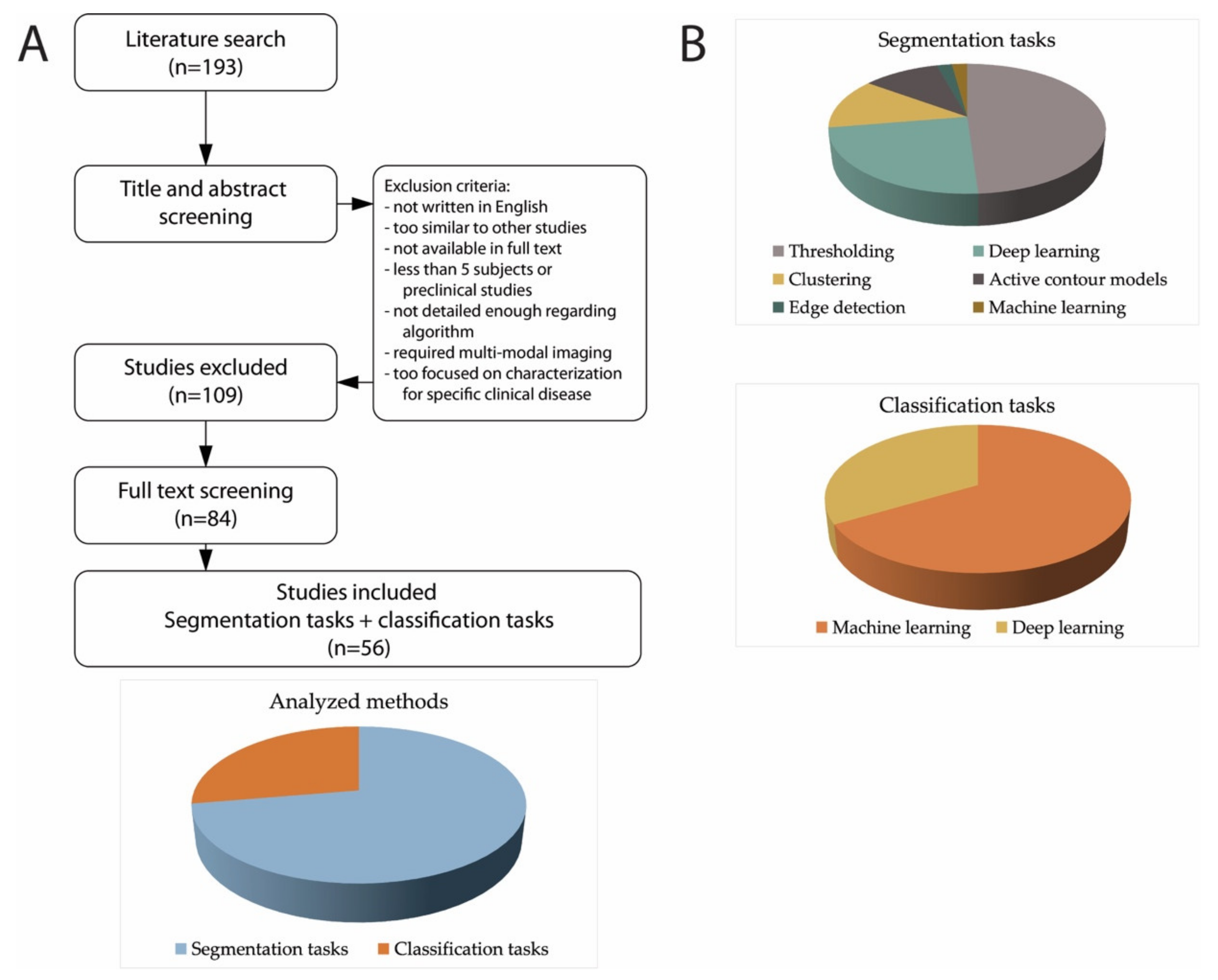
2.1. Literature Search Strategy and Study Selection

The PubMed, Scopus and Google Scholar electronic databases were used between March and August 2021 to find articles that employed an automated method for assessing OCTA images, regardless of the specific application (i.e., DR, dermatology, etc.). The keywords that were used for the electronic database search within the title and/or abstract were as follows: “optical coherence tomography angiography”, “OCTA”, “quantification”, “quantifying”, “segmentation”, “automatic”, “classification”. In particular, the specific query that was used to search was (“optical coherence tomography angiography” OR “OCTA”) AND (“quantification” OR “quantifying” OR “segmentation” OR “automatic” OR “classification”). The database search was limited to initial studies that were published after January 2016. Once the electronic database search was concluded, the reference lists of the identified articles were further analyzed in order to select any additional relevant studies.
Once the initial electronic database search was completed, the articles were screened by reading the titles, the abstracts, and briefly analyzing the Methods section to establish their suitability for inclusion in this review. Specifically, articles were excluded if they (i) were not written in English, (ii) were too similar to other studies, (iii) were not available in full text, (iv) did not enroll a sufficient number of subjects (<5 subjects) or only provided preclinical phantom or animal studies, (v) did not provide enough detail regarding the quantification/classification algorithm or if only a commercial software was employed or if only manual segmentations were employed, (vi) required multi-modal images for the correct implementation of the algorithm (e.g., OCTA image analysis based on fundus image), and (vii) were focused mainly on the characterization of quantitative features for a specific clinical disease and not on the quantitative feature extraction or classification. Furthermore, articles were excluded if they were out-of-topic with respect to the aims of the present review, such as methods or algorithms for the sole purpose of artefact removal for OCTA images. Hence, we excluded studies that focused only on OCTA image preprocessing, and studies that have an OCTA application but use mainly structural OCT data for the method implementation (e.g., retina layer segmentation) [14,15].

2.2. Data Extraction

After the initial database screening, the remaining studies were analyzed individually and the following information was extracted: study title, first author name, year of publication, imaging device used, imaging area field of view (FOV), anatomy of interest (e.g., eye, skin, etc.), if the proposed method had a final aim of segmentation and/or classification, the main category of the method used (e.g., segmentation based on thresholding or clustering, etc.), details of the proposed method, if 2D or 3D data were used, database information, validation methods, and the final performance results. During this process, some initially included studies were removed as after a more detailed analysis, it was found that they did not meet the inclusion criteria (e.g., preclinical murine model studies).
This review and handbook is organized as follows: Section 3 provides an initial overview of the global findings after the literature review and then goes into detail regarding the studies found, dividing them into ones focusing on automatic segmentation methods (Section 3.1) or ones focusing on an automatic classification (Section 3.2). Going into more detail, the segmentation and classification methods are subsequently divided into the main categories that were found to be employed for each individual specific task (i.e., segmentation or classification). Section 4 then discusses the main findings and the future scopes for research and Section 5 provides the conclusions of this review.

3. Results

The initial literature search resulted in finding 193 studies that were screened for title and abstract. After this screening, 109 studies were removed, and the remaining 84 papers were analyzed individually. Figure 3A displays a flowchart of the study selection.
A total of 56 articles were selected for this review and are reported here. Thirty-eight studies (67.9%) focused exclusively on the automatic or semi-automatic segmentation of a structure of interest (e.g., vasculature or foveal avascular zone). The remaining 18 articles (32.1%) had a final goal of classifying the images into pathological or healthy or disease staging, either based on extracting hand-crafted features and then employing a machine learning technique, or end-to-end deep learning methods. A number of studies (n = 9, 16.1%) presented both a segmentation and a classification method, all of which employed a machine learning classification method based on extracted features that first required the segmentation of a structure of interest (e.g., vasculature parameters or the foveal avascular zone (FAZ) area). These 9 studies are included in both Section 3.1 on segmentation tasks and in Section 3.2 on classification tasks, hence making the final number of analyzed studies focusing on segmentation equal to 47. Studies that included the comparison of various segmentation or classification methods (e.g., thresholding vs. machine learning for segmentation) are included in each relevant section.
The methods for segmentation were global or local thresholding (n = 23/47, 48.9%), deep learning (n = 11/47, 23.4%), clustering (n = 6/47, 12.9%), active contour models (n = 5/47, 10.6%), edge detection (n = 1/47, 2.1%), or machine learning (n = 1/47, 2.1%). For classification tasks, machine learning was the majority (n = 12/18, 66.7%) over deep learning techniques (n = 6/18, 33.3%). Figure 3B shows a pie chart of the segmentation and classifications tasks.

3.1. Segmentation Tasks

In this section, the main methods used for the segmentation of structures of interest within the OCTA image are briefly described and compared. When considering ocular applications, the structures of interest that are segmented within the image correspond to either the vasculature or the FAZ. On the other hand, when considering dermatology applications, the structures of interest are mainly the vasculature and, if necessary, the tissue surface. Due to the different segmentation tasks that were found and the importance of comparing different techniques (e.g., thresholding vs. clustering) for one task (e.g., FAZ segmentation), all of the analyzed methods are described in Table 1 and are divided by segmentation task and then by segmentation method. Figure 4 illustrates examples of these segmentation methods.

3.1.1. Thresholding

As can be noted from the large percentage of studies (n = 23, 48.9%), thresholding is the go-to method for segmenting structures of interest in OCTA images. Simply put, it is a method that marks all pixels that have an intensity lower (i.e., darker) or higher (i.e., brighter) than a specifically determined threshold as the object in the obtained binary image. How the intensity threshold is determined can vary greatly and can be divided into two main categories: global or local (also referred to as adaptive).
Global thresholding determines one threshold value for the entire image frame and is determined by an analysis of the whole image intensity histogram. The Otsu method [17] is a commonly used automatic thresholding technique for OCTA images [18,19,20,21,22,23] and is based on finding a threshold that minimizes the intraclass variance of the thresholded black and white pixels. Other global thresholding methods are based on finding a specific percentile of the image intensity histogram [24], the progressive weighted mean of the image intensity histogram [25,26], or by simply fine-tuning a specific gray level [27]. Many analyzed studies employed a global thresholding technique without specifying exactly how the final threshold was determined [22,28,29,30,31,32,33,34].
Local, or adaptive, thresholding is based on analyzing the image in smaller areas, defined by a user-specified neighborhood. A threshold is therefore determined for each pixel, typically using first-order statistics, such as the mean and standard deviation of the pixel intensity within each considered neighborhood. The most commonly found local adaptive thresholding technique in OCTA images is the Phansalkar method [35] which was employed in numerous studies reported in this review [19,34,36,37]. Importantly, Chu et al. [38] provided an interesting outlook on using the Phansalkar thresholding technique for quantifying choriocapillaris, demonstrating the need of careful optimizing of the method’s parameters for an accurate segmentation. Other common local thresholding methods used in OCTA images are the local mean [39] and local median [37,40], and one study employed a signal-to-noise adaptive binarization method [41]. A couple studies used adaptive thresholding without specifying the exact method [30,42].
Thresholding was the most common technique when considering the segmentation task of vasculature, both in ophthalmology and dermatology applications (see Table 1), but it is difficult to compare its performance with other techniques as the majority of the studies did not provide a quantitative validation of the vessel segmentation but rather either continued on to classify a specific disease or compared quantitative parameters computed on the segmentation (healthy vs. pathological subjects) or correlated the parameters with disease staging. The study by Zhang et al. [27] provided a quantitative validation of the obtained segmentation using global thresholding on optimally oriented flux filtered images, showing a Dice coefficient (DSC) equal to 0.8587 for healthy subjects, 0.8434 for proliferative diabetic retinopathy (PDR) subjects, and 0.8520 for severe non-proliferative DR (NPDR) subjects. Although the study was a rare one that employed 3D volumes instead of 2D en face images, the segmentation validation was performed on the 2D projections of the segmentation. Some other studies provided a segmentation comparison with a semi-automated segmentation, such as the one by Meiburger et al. [25], and compared quantitative parameters obtained using the various segmentations (i.e., semi-automatic vs. automatic). This study also provided an intra-operator variability analysis, showing a high variability when using the semi-automatic software for segmentation. When considering the task of segmenting the FAZ, the study by Xu et al. [22] used Otsu thresholding and reaching a maximum DSC equal to 0.90.
Four interesting studies to note when considering thresholding techniques are the work by Rabiolo et al. [43], Laiginhas et al. [19], Terheyden et al. [20], and Mehta et al. [44]. Each of these studies compared several different thresholding techniques for the quantification of OCTA images, and the main finding from each of them is that the absolute quantification values calculated with different thresholding algorithms are not directly interchangeable. Laiginhas et al. found that local thresholding strategies are significantly superior to global ones [19] when considering choriocapillaris and flow deficit parameters. These studies demonstrate how there is still an unmet need for a uniform strategy to quantify OCTA images, and care must be taken when comparing quantitative parameters computed from different thresholded OCTA images.

3.1.2. Deep Learning

Recently, the use of deep learning frameworks for analyzing medical images has seen an exponential growth. Deep learning implies the use of deep neural networks, which is an artificial neural network that has many layers between the input and output layer. Convolutional Neural Networks (CNNs) are specifically used in image analysis applications, as they apply numerous convolutions on the input image [45]. The main advantage of CNNs is that they can automatically learn high-level features and then provide a semantic segmentation by associating each pixel of the input image to a label or class. The drawbacks to deep learning methods are (a) the need of a large annotated database, which has somewhat, but not totally, been mitigated with the employment of transfer learning [46], (b) their complexity (i.e., requirement of an immense number of training parameters) and (c) the difficulty of interaction with any single layer of the network, which can contribute to the view of deep networks as black-boxes that do not explain their predictions in a way that is easily understandable by humans [47].
All of the studies that employed deep learning techniques were based on ophthalmological applications, so either for FAZ segmentation or eye vascular segmentation. This can most likely be explained by the fact that larger databases are available for ocular applications, whereas the dermatological applications are still in the research stage and are not used on a daily basis in a clinical setting. The majority of the studies used already-known architecture styles with some modifications, such as the UNet [11,48,49,50,51,52], VGG [53,54,55], and ResNet [13,56], but two studies also employed custom-made networks [57,58].
The performance of the deep learning methods for eye vasculature segmentation was quite high, as demonstrated by the study by Li et al. [55] that employed a network that took as input the 3D acquired volume and then produced a 2D segmentation using a plane perceptron to enhance the perceptron ability in the horizontal direction. The authors obtained DSC values equal to 0.8941 with images with a 6 × 6 mm2 FOV, and equal to 0.9274 with images acquired on a 3 × 3 mm2 FOV. Another study that showed promising results was by Giarratano et al. that first produced both an open dataset and also provided their source code [11]. Moreover, it provides an interesting comparison between deep learning techniques, specifically the UNet and CS-Net [59], and traditional methods. The best Dice coefficient was obtained using the deep learning methods (DSC = 0.89), yet the traditional adaptive thresholding method on filtered OCTA images also showed high Dice coefficient values (DSC = 0.86). Their study also emphasizes the importance of evaluating segmentation performance in terms of clinically relevant metrics [11]. When considering the FAZ determination, deep learning techniques also outperformed the other methods, as demonstrated by the study by Guo et al. [60] that used a dataset of 405 images and a final DSC value equal to 0.9760. The study by Wang et al. [61] also presented a deep learning method for CNV segmentation, with a maximum Intersection over Union (IoU) equal to 0.88.

3.1.3. Clustering

Clustering is the grouping of similar instances, objects, or pixels in this specific case. In order to group pixels together, there must be some sort of measure that can determine whether they are similar or dissimilar. The two main types of measures used to estimate this relation are distance measures and similarity measures [62].
In the case of OCTA image segmentation, the majority of the analyzed studies used pixel intensity as a way to group together objects, using common methods such as k-means clustering [63,64,65], or other clustering algorithms such as fuzzy c-means clustering [66] and a modified CLIQUE clustering technique [67]. An interesting study that used local features for clustering and not pixel intensity is a method by Engberg et al. [68] which was based on building a dictionary using pre-annotated data and then processing the unseen images by computing the similarity/dissimilarity.
Clustering methods were employed in two clinical applications: general eye vasculature segmentation and choroidal neovascularization (CNV)/Choriocapillaris segmentation. The study by Engberg et al. [68] was a rare study that provided a quantitative validation of general eye vessel segmentation, even though only one image was used for validation. On this image, the DSC was equal to 0.82 for larger vessels and 0.71 for capillaries. For the CNV/Choriocapillaris application, the study by Xue et al. [67] had a final DSC equal to 0.84.

3.1.4. Active Contour Models

The model-based segmentation methods, also known as active contours, can be divided into parametric models, or snakes, and geometric models, which are based on the level set method. These deformable models rely on the definition of both an internal and external energy and an initial contour which evolves until the two energy functions reach a balance.
The five studies that employed a model-based segmentation framework were all focused on ocular applications, either segmenting the retinal vessels [69,70,71] or the FAZ [72,73]. In the first case, the best results were achieved by Sandhu et al. [70] using a database of 100 images and obtaining a final DSC of 0.9502 ± 0.0443. In the same study, the best results were also obtained for FAZ determination, with a DSC equal to 0.93 ± 0.06. Both parametric and geometric active contours were found. One study compared two different ImageJ macros that implement the level set method and the Kanno–Saitama macro [72] with the built-in software for FAZ segmentation, whereas the other three studies used custom-written software implementing the Global Minimization of the Active Contour/Snake model (GMAC) [71], a generalized gradient vector flow (GGVF) snake model [73], and a joint Markov–Gibbs random field (MGRF) model [69].

3.1.5. Edge Detection

Edge detection methods in OCTA images are used rarely as the main segmentation method (n = 1, 2.1%). Briefly, numerous edge detection methods exist, and are based on computing the image gradient, which highlights the sections of the image that present a transition from dark to light or from light to dark along a specific direction.
The study that employed an edge detection method used the Canny method [74], which calculates the gradient using the derivative of a Gaussian filter. The Canny method exploits two thresholds to detect strong and weak edges, including weak edges in the output if they are connected to strong edges. Thanks to the use of these two thresholds, this method is robust to noise and is likely to detect true weak edges. The study using edge detection was found to be employed for determining the FAZ [75] in ocular applications, showing a Jaccard index equal to 0.82. Another study focusing on dermatological applications also employed an edge detection method, but as a preprocessing stage, that is, for determining the tissue surface in skin burn scars [76]. Hence, this type of segmentation method has not been found to segment vasculature, which can be explained by the vasculature complexity and difficulty of detecting connected edges at each angle of the image.

3.1.6. Machine Learning

Machine learning is a type of artificial intelligence technique that is based on the extraction of hand-crafted features which are then fed into a classifier. This method is more commonly used for classification tasks and will be described in more detail in Section 3.2.1, but it can also be employed for segmentation tasks. In this case, the features that are extracted from regions of interest (ROIs) of the image are fed into a classifier to determine whether the current ROI belongs to the object of interest (or to which of the objects of interest they belong in the case of multi-object segmentation) or to the background.
A machine learning method for a segmentation task was found in only one of the analyzed articles and was focused on the choriocapillaris segmentation [77]. The method was based on the extraction of features from the structural OCT images and the inner retinal and choroidal angiograms. In particular, the features included the standard deviation and directional Gabor filters at multiple scales which were then fed into a random forest classifier. This technique showed a final Jaccard index equal to 0.81 ± 0.12.
Table 1. Segmentation tasks summary.
TaskMethodFirst
Author (Year)
Database
2D/3D
Field of View (FOV)
DescriptionResults
Eye
vasculature
ThresholdingChu 2016 [39]5 subjects
2D
6.72 × 6.72 mm2
Global threshold to remove FAZ, Hessian filter, local mean adaptive threshold, skeletonization.No segmentation validation. Repeatability and usefulness of parameters.
Kim 2016 [40]84 DR, 14 healthy
2D
3 × 3 mm2
Global threshold to remove FAZ, Hessian filter, local median adaptive threshold—top hat filter and combination of binarized images.No segmentation validation. Negative correlation between DR severity and SD, VD, FD; positive correlation with VDI.
Alam 2017 [28]36 SCR patients, 26 healthy
2D
3 × 3 mm2
Global thresholding, morphological functions, and fractal dimension analysis.No segmentation validation.
Avascular density was more sensitive to SCR presence than vessel tortuosity and mean diameter.
Ong 2017 [29]38 glaucoma, 120 non glaucoma
2D
6 × 6 mm2
Global thresholding, morphological dilation, closing.No segmentation validation.
Method proposed for classification.
Aharony 2019 [21]20 DR, 6 AMD, 4 RVO, 26 healthy
2D
3 × 3 mm2
Frangi filter, Otsu thresholding.No segmentation validation.
Method proposed for classification.
Alam 2019a [30]100 images/50 subjects
2D
8 × 8 mm2
bias field correction, matched filtering method, bottom hat filtering, global thresholding + adaptive thresholding, morphological operations.No segmentation validation.
Method proposed for classification.
Alam 2019b [42]60 DR, 90 SCR, 40 healthy
2D
6 × 6 mm2
Frangi filter, adaptive thresholding with morphological functions, skeletonization.No segmentation validation.
Method proposed for classification.
Pappelis 2019 [31]30 healthy
2D
6 × 6 mm2
Local Otsu thresholding for all vessels, big blood vessels masked out through Frangi and global thresholding.No segmentation validation.
Repeatability of vessel density and flux.
Xu 2019 [22]123 DR, 108 healthy
2D
6 × 6 mm2
Multi-scale line detector, Otsu thresholding for large vessel segmentation. Frangi Hessian filter and global thresholding for all vessels segmentation, skeletonization.No segmentation validation. Repeatability and differences between healthy and diseased.
Abdelsalam 2020 [32]30 DR, 30 NPDR, 40 healthy
2D
3 × 3 mm2
Contrast and resolution enhancement, Frangi filter, global thresholding.No segmentation validation.
Method proposed for classification.
Andrade De Jesus 2020 [24]82 glaucoma, 39 healthy
2D
3 × 3 mm2
Microvasculature: Foveal disc axis correction, global thresholding (88th percentile of image intensity histogram), morphological opening and closing, small object removal.
Choroid: global thresholding (lower 40th percentile), keep largest connected component.
No segmentation validation.
Method proposed for classification.
Borrelli 2020 [34]15 NPDR, 15 healthy
3D
3 × 3 mm2
Projection removal algorithm, global default thresholding.No segmentation validation. The 3D vascular volume and 3D perfusion density were reduced in DR eyes.
Mehta 2020 [44]13 healthy
2D
3 × 3 mm2
Histogram normalizatioon, CLAHE, linear registration.11 binarization techniques: global default, global Huang, global IsoData, global mean, global Otsu, local Bernsen, local mean, local median, local Niblack, local Otsu, and local Phansalkar.No segmentation validation. No thresholding method is highly repeatable across contrast changes. Quantification is more repeatable when using local thresholds.
Su 2020 [37]25 high myopic, 25 moderate, 25 healthy
2D
6 × 6 mm2
Binarization through combination of (1) Hessian filter, Huang’s fuzzy thresholding method, (2) median local thresholding.No segmentation validation. Flow deficit evaluation (mean subfoveal choroidal thickness).
Terheyden 2020 [20]26 images
2D
-
Comparison between Manual, Huang, Li, Otsu, Moments, Mean, Percentile thresholding techniques.No segmentation validation. Reproducibility was higher with automated methods vs. manual.
Zhang 2020 [27]20 NPDR, 40 PDR, 40 controls
3D
3 × 3 × 2 mm3
Curvelet denoising and optimally oriented flux (OOF) filtering, global thresholding (threshold = 0.14).DSC = 0.8587 for normal, 0.8520 for severe NPDR, 0.8434 for PDR, using 2D projections.
Abdelsalam 2021 [33]80 DR, 90 healthy
2D
3 x 3 mm2
Contrast and resolution enhancement, global thresholding.No segmentation validation.
Method proposed for classification.
Wu 2021 [23]14 subjects
2D
6 × 6 mm2
Matched filtering vs. preprocessing: image cropping and color space conversion, Otsu thresholding, skeletonizationo, artefacts elimination.No segmentation validation.
Analysis of NVC with PRD treatment.
ClusteringKhansari 2017 [64]41 subjects
2D
3 × 3 mm2 & 6 × 6 mm2
K-means clustering for segmentation, morphological operators.No segmentation validation.
Vessel tortuosity index comparison and correlation.
Engberg 2019 [68]10 patients, 10 healthy
2D
3 × 3 mm2
Dictionary-based method using pre-annotated data and then processing unseen imagesOn one validation image:
DSC = 0.82 for larger vessels, 0.71 for capillaries, and 0.76 for background.
Cano 2020 [65]33 no DR, 26 mild NPDR, 13 PDR, 22 healthy
2D
6 × 6 mm2
K- means clustering.No segmentation validation.
Method proposed for classification.
Chavan 2021 [63]41 subjects
2D
6 × 6 mm2
Multiscale and multi span line detectors, k-means clustering into 2 classes, morphological closing.No segmentation validation.
Comparison between parameters and male and female, age, etc.
Active
Contour
Models
Eladawi 2017 [69]24 diabetic, 23 healthy
2D
6 × 6 mm2
GGMRF model for contrast improvement, joint Markov Gibbs model to segment, hOMGRF moodel to overcome low contrast, segmentation refinement with 2D connectivity filter.DSC = 0.9504 ± 0.0375
Sandhu 2018 [70]82 mild DR, 23 healthy
2D
6 × 6 mm2
GGMRF model for contrast improvement, joint Markov Gibbs model to segment, hOMGRF moodel to overcome low contrast, segmentation refinement with 2D connectivity filter.DSC = 0.9502 ± 0.0443
Wu 2020 [71]30 images
2D
3 × 3 mm2
Stripe removal and segmentation using global minimization of the active contour model (GMAC).Accuracy = 0.93
Deep LearningPrentasic 2016 [58]80 images/6 subjects
2D
1 × 1 mm2
Custom architecture: Square filters convolutions (ReLU), max pooling, dropout layer, two fully connected layers, final fully connected layer. Three fold cross validation.Mean accuracy = 0.83
F1 measure = 0.67
Giarratano 2020 [11]50 ROIs on images
2D
6 × 6 mm2
UNet, CS-NET + thresholding, morphological opening.UNet DSC = 0.89
CS-Net DSC = 0.89
Li 2020 [54]316 volumes
3D to 2D
6 × 6 × 2 mm3
VGG projection learning module (unidirectional pooling layer). Input 3D data and output 2D segmentation.DSC = 0.8815
Lo 2020 [50]Test: 28 DR, 8 healthy
2D
6 × 6 mm2
UNet variation, adapted for vessel and background. Fine-tuned network using a transfer learning method.SCP DSC = 0.8599
DVC DSC = 0.7986
Pissas 2020 [51]50 subjects
2D & 3D
8 × 8 mm2
UNet modified architecture with iterative refinement (stacked hourglass network SHN distinct cascaded UNet modules, and single network employed by recurrently feeding intermediate predictions in the network to obtain refined predictions (iUNet).DSC = 0.8540
Ma 2021 [13]229 images
2D
3 × 3 mm2
OCTA-Net: ResNet style. Coarse stage (split-based coarse segmentation (SCS) module to produce preliminary confidence maps) and fine stage (split-based refined segmentation (SRS) module to fuse vessel confidence maps to produce the final optimized results).SVC DSC = 0.7597
DVC DSC = 0.7074
Both DSC = 0.7576
Li preprint [55]500 images
3D to 2D
3 × 3 mm2 & 6 × 6 mm2
IPN-V2: addition of plane perceptron to enhance the perceptron ability in the horizontal direction + global retraining. 3D volume to 2D segmentation.6x6 DSC = 0.8941
3x3 DSC = 0.9274
Yu 2021 [52]80 images
2D to 3D
3 × 3 mm2
Structure-constraint UNet architecture with feature encoder module, feature decoder module, and structure constraint blocks (SCB) for depth map estimation. From 2D segmentation to 3D space.No segmentation validation.
Depth prediction method is validated.
Foveal Avascular Zone (FAZ)ThresholdingAlam 2017 [28]36 SCR, 26 healthy
2D
3 × 3 mm2
Global thresholding, morphological functions, and fractal dimension analysis.No segmentation validation.
FAZ contour irregularity was more sensitive to SCR presence then FAZ area.
Xu 2019 [22]123 DR, 108 healthy
2D
6 × 6 mm2
Multi-scale line detector, Otsu thresholding for large vessel segmentation. Frangi Hessian filter and global thresholding for all vessels segmentation, skeletonization.DSC = 0.90
Edge
detector
Diaz 2019 [75]213 subjects
2D
3 × 3 mm2 & 6 × 6 mm2
Morphological operators, white top-hat operator, Canny edge detector, morphological closing, inversion, removal of small objects.Jaccard = 0.82
Active
Contour
Models
Lu 2018 [73]66 DR, 19 healthy
2D
3 × 3 mm2
GGVF snake model.Jaccard =
0.87 ± 0.06 (healthy)
0.86 ± 0.09 (diabetes with DR)
0.89 ± 0.05 (mild NPDR)
0.83 ± 0.09 (sever NPDR or PDR)
Sandhu 2018 [70]82 mild DR, 23 healthy
2D
6 × 6 mm2
GGMRF model for contrast improvement, joint Markov Gibbs model to segment, hOMGRF moodel to overcome low contrast, segmentation refinement with 2D connectivity filter.DSC = 0.93 ± 0.06
Lin 2020 [72]20 training / 37 test
2D
3 × 3 mm2
Level Set model (ImageJ).DSC = 0.9243
Deep learningGuo 2019 [60]405 images
2D
3 × 3 mm2
UNet, thresholding and largest connected region extraction and hole filling.DSC = 0.9760
Li 2020 [54]316 volumes
3D to 2D
6 × 6 × 2 mm3
VGG projection learning module (unidirectional pooling layer). Input 3D data and output 2D segmentation.DSC = 0.8861
Guo 2021 [57]80 subjects
2D
3 × 3 mm2
Normalization, custom made network: boundary alignment module (BAM) implemented to extract global information.DSC = 0.88
Li preprint [55]500 images
3D to 2D
3 × 3 mm2 & 6 × 6 mm2
IPN-V2: addition of plane perceptron to enhance the perceptron ability in the horizontal direction + global retraining. 3D volume to 2D segmentation.6x6 DSC = 0.9084
3x3 DSC = 0.9755
CNV / ChoriocapillarisThresholdingCheng 2019 [18]17 CNV
2D
-
CIELAB color space transformation, Otsu thresholding, majority, size filter.No segmentation validation.
Discussion of features
Laiginhas 2020 [19]18 images
2D
-
Projection artefact removal, local thresholding (Phansalkar, mean, Niblack) and global thresholding (mean, default, Otsu).No segmentation validation.
Local thresholding methods are more robust and reproducible.
ClusteringTaibouni 2019 [66]54 patients
2D
3 × 3 mm2
Frangi filter, Gabor wavelets and fuzzy c-means classification.No segmentation validation.
Quantitative parameters compared with manual software.
Xue 2019 [67]48 AMD
2D
-
Global threshold (0.3), median filter, grid tissue-like membrane system modified CLIQUE clustering algorithm.DSC = 0.84
Machine learningGao 2017 [77]30 images/19 CNV
2D
6 × 6 mm2
Random forest classifier (structural OCT images, inner retinal and choroidal angiograms, standard deviation, and directional Gabor filters at multiple scales).Jaccard = 0.81 ± 0.12
Deep learningWang 2020 [61]Test 100 CNV, 120 non-CNV
2D
3 × 3 mm2
Custom CNNs: one for CNV membrane identification and segmentation and one for pixel wise vessel segmentation.Max IoU = 0.88
Skin vasculatureThresholdingLiew 2012 [76]8 scar patients
2D MIP
4 × 1.5 × 3 mm3
Tissue surface segmentation (Canny edge), global thresholding, skeletonization.No segmentation validation.
Parameter analysis for normal vs. scar tissue
Meiburger 2019 [25]7 BCC patients
3D
10 x 10 x 1.2 mm3
Frangi, global thresholding per image slice, adaptive among volume, skeletonization.Validation of parameters vs semi-automated segmentation.
High intra-operator variability for semi-automatic segmentation.
Zhang 2020 [41]10 subjects–2 sites
3D
2.5 × 2.5 × 2.5 mm3
ID-BISIM threshold: SNR adaptive binarization method based on the linear boundary of static signals in ID spaceSensitivity = 0.83 ± 0.15
Specificity = 0.98 ± 0.01
CNV: choroidal neovascularization; SD: skeleton density; VD: vessel density; FD: fractal dimension; VDI: vessel diameter index; SCR: sickle cell retinopathy; DR: diabetic retinopathy; NPDR: non-proliferative diabetic retinopathy; AMD: age-related macular degeneration; DSC: Dice Coefficient; SCP: superficial capillary plexus; DVC: deep vascular complex; SVC: superficial vascular complex; IoU: Intersection over Union; BCC: basal cell carcinoma; 3.2. Classification tasks.

3.2. Classification Tasks

In this section, the main methods used for the classification of OCTA images are briefly described and compared. There were no studies found that focused on the classification of skin vasculature, so all analyzed studies aimed at classifying ocular OCTA images. The main focus of classification tasks were the detection of retinal diseases, such as DR, AMD, glaucoma, and choroideremia. Two analyzed studies instead focused on the classification between arteries and veins within the OCTA image, which can provide important information for early disease detection and better stage classification [30,78]. Due to the different classification tasks that were found and the importance of comparing different techniques (i.e., machine learning vs. deep learning) for one task (e.g., DR detection), all of the analyzed methods are described in Table 2 and are divided by classification task and then by classification method. Figure 5 illustrates examples of how these classification methods work.

3.2.1. Machine Learning

Machine learning is an artificial intelligence technique that is based on the extraction of hand-crafted features which are then fed into a classifier, such as neural networks (NNs), support vector machines (SVM), or random forests (RF) [79].
In the context of retinal diseases, a recent review has been presented in literature that analyzes the quantitative parameters of retinal OCTA images that have been used in numerous studies [12]. Briefly, the main quantitative parameters that have been used are: blood vessel tortuosity (BVT), blood vessel caliber (BVC) or vessel diameter, blood vessel density (BVD or just VD), vessel perimeter index (VPI), foveal avascular zone area (FAZ-A), foveal avascular zone contour irregularity (FAZ-CI), vessel complexity index (VCI) such as the fractal dimension (FD), branchpoint analysis (BPA), differential artery–vein (A–V) analysis, flow analysis using parameters such as the flow index (FI) or flow void (FV), vessel branching coefficient, vessel branching angle, branching width ratio, and choroidal neurovascular (CNV) analysis. The mathematical description of these quantitative parameters is out of scope of this review, so interested readers can refer to the study by Yao et al. [12] for a comprehensive analysis and definition of these parameters in quantitative OCTA image analysis. These quantitative parameters are based on the segmentation of the FAZ or of the blood vessels. When considering the vasculature parameters listed above, they are typically computed not on the output segmented image or volume but a thinning technique, often called skeletonization [80], is rather applied to the vessel segmentation. This method reduces the vasculature to a centerline of the vessels and has been used in numerous other studies and imaging modalities [81,82].
A few studies instead computed texture features, such as those based on a local binary pattern (LBP) analysis [83] or the wavelet transform [84], and either used only these features for classification or combined them with other standard quantification parameters that were previously listed.
The most common machine learning method that was found for OCTA image classification was the support vector machine (SVM) [85]. This classifier was used for single disease detection, such as DR [70,84] and glaucoma [24,29], and was also employed for more complex classification tasks, such as DR staging [33] and distinguishing between different retinopathies [42]. The other classifiers that were used were NNs [32,83,86], k-means clustering [42], logistic regression [84], and a gradient boosting tree (XGBoost) [84].
Machine learning classification methods were used in basically all clinical applications, which included DR classification and staging, glaucoma classification, AMD classification, artery/vein classification, sickle cell retinopathy (SCR) classification and general retinopathy classification. When considering a general retinopathy classification, the study by Alam et al. [42] used the features extracted from different areas (BVT, BVC, VPI, BVD, FAZ) and FAZ contour irregularity features within an SVM classifier and obtained a maximum accuracy of 97.45% when classifying between healthy and diseased images. When considering the different pathologies, the accuracy was slightly lower: 94.32% (DR vs. SCR). Alam et al. [87] also presented a study for SCR classification, using the same features of Alam et al. [42] and three different classifiers: SVM, KNN, and discriminant analysis. The best results were obtained using an SVM classifier, with a final accuracy equal to 97%. Again, Alam at el. [30] presented a study also for artery/vein classification using a k-means clustering method, presenting an accuracy equal to 96.57% when considering all vessels. When considering AMD classification, Alfahaid et al. [83] used rotation invariant uniform local binary pattern texture features computed on 184 images couple with a KNN classifier to obtain a maximum accuracy of 100% when considering the choriocapillaris layer, and an accuracy of 89% for all layers. For glaucoma classification, Ong et al. [29] presented a promising study using Haralick’s texture features and other global and local features which were then classified using an SVM to obtain an Area Under the Curve (AUC) equal to 0.98, considering a database of 158 images (38 glaucoma). When considering DR classification, which is the most commonly found clinical application in the analyzed studies, the most promising results were presented by Abdelsalam et al. [33], using multifractal parameter computation with an SVM classifier which showed an accuracy of 98.5% computed on a database of 80 DR patients and 90 healthy subjects.

3.2.2. Deep Learning

As mentioned in Section 3.1.2, deep learning implies the use of deep neural networks, and typically CNNs for image analysis. CNNs can automatically learn high-level features from the input image and therefore have the advantage of not requiring the extraction of hand-crafted features for classification [88], simply needing the input image and the correct class to which it belongs. The drawbacks of deep learning for classification are the same as those mentioned for segmentation tasks in Section 3.1.2. An advantage that classification tasks have over segmentation tasks when considering deep learning is the fact that it is typically less painstaking to obtain the expert ground truth, since manual segmentations can be very time consuming and require the usage of basic image processing software whereas manual classification of images is usually quicker and easier.
For OCTA image classification, deep learning methods were employed for artery/vein classification [78], DR detection [86,89,90], AMD detection and staging [91], and chorioretinopathy detection [92]. The architectures that were employed included UNet [48], VGG16 and VGG19 [53], ResNet50 [56], and DenseNet [93]. All of the networks took as input a 2D image, with the exception of the work by Thakoor et al. [91] that did not use the 3D acquired volume but stacked 2D images of the retinal layers of interest, obtaining a 93.4% testing accuracy at binary classification of neovascular AMD vs. non-AMD.
Deep learning methods were employed in many clinical applications of classification tasks: DR classification, AMD classification, artery/vein classification, and Central Serous Chorioretinopathy (CSC) classification. Aoyama et al. [92] presented a deep learning method based on a VGG16 pretrained model for CSC classification and obtained a final accuracy of 95%. For artery/vein classification, Alam et al. [78] used a fully connected network based on the UNet for classifying 30 DR and 20 healthy images, obtaining an accuracy equal to 86.75%, showing lower performances than those presented by the same authors [42] using a machine learning technique (accuracy = 96.57%). When considering AMD classification, Thakoor et al. [91] presented an interesting study employing a custom-made 3D CNN and using as input a stack of 2D images of retinal layers of interest. When using a two-class classification (i.e., NV-AMD vs. healthy), the classification accuracy was quite high (93.4%), but when considering a three-class classification (NV-AMD vs. non-NV-AMD vs. healthy), the accuracy decreased (77.8%). For DR classification, numerous approaches were presented, and the most promising was the study by Zang et al. [90] that used a densely and continuously connected neural network with adaptive rate dropout. The obtained accuracy was equal to a maximum of 96.5% for two-class classification and minimum 67.9% considering a four-class classification. Another study to note is the one by Heisler et al. [86] that employed an Ensemble network and obtained an accuracy equal to 92 ± 1.92%. Higher accuracy values were obtained using a machine learning method [33]; however, it must also be pointed out that the databases in the deep learning methods are also almost double or triple in size.
Table 2. Classification tasks summary.
TaskMethodFirst Author (Year)Database
2D/3D
Field of View (FOV)
DescriptionResults
Diabetic
retinopathy
classification
Machine
learning
Sandhu 2018 [70] 82 DR, 23 healthy
2D
6 × 6 mm2
Features: blood vessel density, blood vessel caliber, distance map of FAZ area.
Classifier: SVM classifier with RBF.
AUC = 95.22%
Aharony 2019 [21]20 DR, 6 AMD, 4 RVO, 26 healthy
2D
3 × 3 mm2
Features: mean, standard deviation, skewness, and kurtosis of gray level histogram.
No formal classifier.
Accuracy = 83.9%
Abdelsalam 2020 [32]30 DR, 30 NPDR, 40 healthy
2D
3 × 3 mm2
Features: mean of the intercapillary areas, FAZ perimeter, circularity index, and vascular density.
Classifier: neural network
Total Accuracy = 97%
Precision =
95.2% (healthy vs. diabetic)
96.7% (DR vs. NPDR)
Cano 2020 [65]33 no DR, 26 mild NPDR, 13 PDR, 22 healthy
2D
6 × 6 mm2
Features: Vessel tortuosity, fractal dimension ratio (FDR).
Classifier: Ordinary least squares modeling method.
PDR Accuracy = 94%
Mild NPDR vs. healthy
Accuracy = 91%
Abdelsalam 2021 [33]80 DR, 90 healthy
2D
3 × 3 mm2
Features: multifractal parameter computation (maximum, shift, width, lacunarity, box counting dimension, information dimension, correlation dimension).
Classifier: SVM.
Accuracy = 98.5%
Liu 2021 [84]114 DR, 132 healthy
2D
3 × 3 mm2
Features: wavelet transform on SVP, DVP, RVN.
Classifiers: LR, LR-EN, SVM, XGBoost.
Sensitivity = 84%
Specificity = 80%
Deep
learning
Heisler 2020 [86]463 volumes
2D
3 × 3 mm2
VGG19, ResNet50, and DenseNet with superficial and deep plexus images, majority soft voting.Ensemble network
accuracy = 92 ± 1.92%
Le 2020 [89]75 DR, 24 diabetes, 32 healthy
2D
6 × 6 mm2
VGG16.Accuracy = 87.27%
AUC =
0.97 (healthy)
0.98 (no DR)
0.97 (DR)
Zang 2021 [90]303 images
2D
3 × 3 mm2
A densely and continuously connected neural network with adaptive rate dropout (DcardNet).Accuracy =
96.5% (two class)
80.0% (three classes)
67.9% (four classes)
Glaucoma
classification
Machine
learning
Ong 2017 [29]38 glaucoma, 120 healthy
2D
6 × 6 mm2
Features: Haralick’s texture features, inverse difference normalized and inverse difference moment normalized features, global features (including mean, standard deviation, skewness, kurtosis, and entropy), local structure features, thresholded cumulative count of microvasculature pixels).
Classifier: SVM.
Specificity = 0.95
Sensitivity = 0.87
AUC = 0.98
Andrade De
Jesus 2020 [24]
82 glaucoma, 39 healthy
2D
3 × 3 mm2
Features: microvascular intensity median computed on 6 layers and 7 sectors.
Classifiers: SVM, random forest, and gradient boosting.
AUC = 0.76± 0.06 (xGB)
AUC = 0.67± 0.06 (RNFL)
Age-Related Macular
Degeneration Classification
Machine
learning
Alfahaid 2018 [83]92 AMD, 92 healthy
2D
-
Features: rotation invariant uniform local binary pattern texture features.
Classifier: KNN classifier
Accuracy =
89% (all layers)
89% (superficial)
94% (deep)
98% (outer)
100% (choriocapillaris)
Deep
learning
Thakoor 2021 [91]160 non-NV-AMD, 80 NV-AMD, 97 healthy
2D
-
Custom-made 3D CNN, consisting of 4 3D convolutional layers, two dense layers, and final softmax classification.Accuracy =
93.4% (NV-AMD vs. healthy)
77.8% (NV-AMD vs. non-NV-AMD vs. healthy)
Artery/vein
classification
Machine
learning
Alam 2019 [30]100 images
2D
8 × 8 mm2
Features: ratio of vessel width to central reflex, average of maximum profile brightness, average of median profile intensity, optical density of vessel boundary intensity compared to background intensity.
Classifier: K-means clustering
All vessel
Sensitivity = 0.9679
Specificity = 0.9572
Accuracy = 96.57%
AUC = 98.05%
Deep
learning
Alam 2020 [78]30 DR, 20 healthy
2D
6 × 6 mm2
Enface fully connected network based on UNetAccuracy = 86.75%
Central Serous Chorio-
retinopathy
classification
Deep
learning
Aoyama 2021 [92]53 CSC, 47 healthy
2D
12 × 12 mm2
VGG16 pretrained modelAccuracy = 95%
Sickle cell
retinopathy
classification
Machine
learning
Alam 2017 [87]35 SCD, 14 healthy
2D
-
Features: BVT, BVC, VPI, FAZ area, FAZ contour irregularity, PAD.
Classifiers: SVM, KNN, discriminant analysis
Accuracy =
97% (SVM)
95% (KNN)
88% (discriminant analysis)
Retinopathy classificationMachine
learning
Alam 2019 [42]60 DR, 90 SCR, 40 healthy
2D
6 × 6 mm2
Features: BVT, BVC, VPI, BVD, FAZ area, FAZ contour irregularity.
Classifier: SVM
Accuracy =
97.45% (healthy vs. disease) 94.32% (DR vs SCR)
89.60% (NPDR staging)
93.11% (SCR staging)
SVP: superficial vascular plexus; DVP: deep vascular plexus; RVN: retinal vascular network; LR: logistic regression; LR-EN: logistic regression regularized with the elastic net penalty; SVM: support vector machine; DR: diabetic retinopathy; AMD: age-related macular degeneration; RVO: retinal vein occlusion; NPDR: non proliferative DR; PDR: proliferative DR; xGB: gradient boosting; RNFL: retinal nerve fiber layer; NV-AMD: neovascular AMD; BVT: blood vessel tortuosity; BVC: blood vessel calibre; BVD: blood vessel density; VPI: vessel perimeter index; FAZ: foveal avascular zone; PAD: parafoveal avascular density;4. Discussion.

4. Discussion

In this review and handbook, we aimed to provide the reader with an overview of the most common segmentation and classification methods that are employed for automatic OCTA image or volume analysis. In this section, some key findings and future prospects are discussed.
A first find is that the vast majority of studies (53 out of 56, 94.6%) focus on ocular applications, which can be explained by the fact that there are numerous clinical devices available for this specific field. The main clinical devices that were used in the analyzed studies were the: (a) Avanti OCTA system (Optovue, Inc., Fremont, CA, USA), (b) DRI OCT Triton or DRI OCT-1 Triton plus, (Topcon Medical Systems, Paramus, NJ, USA), and (c) PLEX Elite or Cirrus system (Carl Zeiss Meditec, Dublin, CA, USA). Three (5.4%) studies instead focused on the analysis of OCTA data acquired on human skin, two of which used custom-made laboratory OCT/OCTA systems [25,41] and one of which employed a fiber-based swept-source polarization-sensitive OCT system (PSOCT-1300, Thorlabs) [76]. Hence, it can be observed how the use of OCTA imaging is quite established for ocular applications, but it is starting to move in other interesting directions, such as the non-invasive analysis of vasculature in skin. The fact that the upcoming research field of OCTA imaging is found in dermatology can be explained by the fact that the limited penetration depth of OCT/OCTA imaging makes the analysis of superficial vasculature an ideal application.
A second important overall aspect to discuss is the type of data analyzed, either two-dimensional or three-dimensional. The acquired OCTA data from devices are inherently three dimensional, yet the vast majority of studies employ segmentation or classification methods on 2D images instead of the 3D volumes. The 2D images are typically obtained as a Maximum Intensity Projection (MIP) en face image of a specific retinal layer in the case of ocular applications, or of the entire acquired volume in the case of dermatological applications. A few recent studies have instead employed algorithms using the acquired volumetric data, in both ophthalmological and dermatological applications [27,29,36,53]. To note is an interesting study by Yu et al. [52] that employs a structure-constraint CNN architecture for a depth map estimation to map a segmentation obtained on 2D images into a 3D space. Especially when considering the up and coming research field of OCTA imaging in dermatology applications, the usage of the 3D volume should be considered preferable as it can provide an important 3D visualization of the vasculature and, more importantly, a more accurate vascular analysis and quantification [1].
A third overall aspect to take into consideration is the imaging area FOV. Considering a scan step size that is proportional to the FOV, the scan density for a smaller FOV (e.g., 1 × 1 mm2) is higher than that for a larger FOV (e.g., 12 × 12 mm2), providing a better scan resolution and hence a better ability to delineate detailed microvasculature. On the contrary, a larger FOV covers a wider area of scan coverage and is hence more likely to detect the presence or absence of pathological features such as non-perfusion and microaneurysms [94]. The FOV in the analyzed studies (not considering the depth which was not always reported) ranged from 1 × 1 mm2 up to 12 × 12 mm2. For ocular applications, most of the studies employed a FOV equal to 3 × 3 mm2 or 6 × 6 mm2, with only three studies employing a larger FOV and one study employing a smaller FOV. Interestingly, each of these four studies adopted either machine learning or deep learning techniques for segmentation and/or classification. For skin applications, the imaging FOV varied and was not consistent throughout the three analyzed studies, employing both a small FOV (i.e., 2.5 × 2.5 mm2) and a larger FOV (i.e., 10 × 10 mm2). When 3D volumes were analyzed, the scanning depth ranged from 1.2 mm to 3 mm.
In this review, preprocessing methods for enhancing OCTA images and postprocessing methods for improving the segmentation or classification results were not taken into consideration. Preprocessing and postprocessing methods can improve segmentation and classification outcomes. This has been demonstrated both with traditional techniques on OCTA images, such as thresholding [36], and with deep learning methods in digital pathology, which can also be extended to other research fields [95]. In OCTA imaging, the most commonly found preprocessing steps are those focusing on vessel enhancement. These filters aim to enhance structures within the image or volume that appear to have a vessel-like structure and reduce the signal if not. The most commonly used vesselness filter found in literature is the one proposed by Frangi et al., known as the Frangi filter [96]. This filter is characterized by a scale parameter that determines the dimensions of the vessels that are recognized and then enhanced in the image/volume. It is also possible to combine multiscale measurements (i.e., combine different scale parameter values) and hence recognize both smaller and larger vessels. Other common filters for vessel enhancement include the optimally oriented flux (OOF) filter [97], Gabor [98], and SCIRD-TS [99]. All of these filters also require parameter tuning similar to the Frangi filter. The next common preprocessing method is histogram normalization and contrast enhancement using methods such as CLAHE [100]. When considering 3D volumes, an important preprocessing method is projection artefact removal, a common OCTA artefact that causes the signal from a superficial vessel to protrude deeper within the volume than it should [101]. Numerous techniques for projection artefact removal have been proposed in literature [102]. One analyzed study combined stripe removal, another common artefact in OCTA images, with an active contour model [71]. Regarding segmentation postprocessing methods, the main techniques that were used were hole filling, small object removal and morphological operators to smooth the final boundaries.
Another important factor to note is the difficulty of direct comparisons between studies. This can be observed when considering quantitative parameters obtained using different segmentation techniques, which has been accurately demonstrated for various thresholding methods [21,45,46], but can be extended to include any segmentation technique. Any segmentation method that is used will provide a different final binary image and therefore will change, even if only slightly, the obtained quantitative parameter. As mentioned previously, this calls for the dire need of a consensus across the research community for OCTA image quantification. This can be partially attributed to the fact that the majority of the studies that presented an automated technique for combined segmentation and classification using quantitative parameters did not actually validate the segmentation method against a manual segmentation but only validated the final classification results with a manual classification. Other studies that presented a segmentation technique did not actually validate the obtained segmentation but rather focused on the repeatability of the measurements, such as the studies by [21,33,41,46], or on the statistical differences or correlation between quantitative parameters obtained on images from healthy and pathological subjects, such as the studies by [36,42,78]. Another comparison difficulty is simply the fact that almost all studies used proprietary databases. Fortunately, the open science movement has recently also reached OCTA imaging applications in the ophthalmological field, and a few recent studies provide not only a segmentation method for retinal OCTA images but also an open dataset. Specifically, Giarratano et al. [11] published the first open dataset of retinal parafoveal OCTA images with their associated ground truth manual segmentations, including a database of 55 ROIs from OCTA images acquired on 11 subjects. Yuhui et al. [13] presented the ROSE dataset that contains 229 OCTA images with vessel annotations at either centerline-level or pixel level, and Mingchao et al. [55] presented the OCTA-500 method and dataset which contains data acquired on 500 subjects with two FOV types. The dataset includes both OCT and OCTA volumes, six types of projections, four types of text labels, and two types of pixel-level labels. Very recently, a preprint by Untracht et al. [103] was made available that presents OCTAVA, an open-source toolbox for the quantitative analysis of optical coherence tomography angiography images. The authors present a Matlab GUI to help automate the quantitative analysis of en face OCTA maximum intensity projection images in a standardized workflow, including preprocessing, segmentation, and quantitative parameter computation steps. Thanks to these datasets and tools and the trend of making datasets and also automatic methods open for researchers to use, the problem of a lack of consensus should be mitigated in the coming years.
Among the methods that presented a segmentation validation, from Table 1 it can be seen how the methods that employed a thresholding technique were mainly also those that did not present any segmentation validation, but rather focused the study on the analysis of specific parameters obtained from the segmentation with a clinical aspect. On the other hand, the other segmentation methods tend to include a validation of the segmentation and are more strictly focused on the presentation of a unique segmentation algorithm. When considering a complicated segmentation task, such as vasculature segmentation, the GGMRF models by Eladawi et al. [69] and Sandhu et al. [70] show very promising results, with a DSC equal to 0.95, but are limited to a database of slightly over 100 images. The more recent deep learning methods include much larger databases, such as the one presented by Li et al. [55] which includes 500 images and shows very promising results (DSC = 0.9274) when considering a 3 × 3 mm2 FOV. When considering easier segmentation tasks, such as the FAZ segmentation, it can be observed how the highest state-of-the-art segmentation results are reached only by deep learning methods, showing a 5–10% increase in segmentation performance parameters.
From the methods analyzed in this review, it can be observed that machine learning methods are still the majority and also typically present the highest performance results for now, in terms of accuracy, when considering classification tasks. For example, for diabetic retinopathy classification, the highest accuracy was obtained by Abdelsalam et al. [33], reaching a 98.5% accuracy on a database of 170 images using an SVM classifier. Still, the DcardNet presented by Zang et al. [90] showed very similar, albeit slightly lower, results with a 96.5% accuracy on a dataset that was almost twice the size (303 images). Overall, what can be observed with both machine learning and deep learning classification methods is that, as the classification task increases in complexity (e.g., disease staging or multiple disease classification), the obtained classification results tend to decrease when using a similar-sized dataset, which can be expected.
Quantitative OCTA imaging and the employment of automatic segmentation and classification methods is an emerging field, with a solid basis of various techniques for ophthalmological applications and the beginnings of a foundation of methods for dermatological applications. Although still the minority in literature for ocular applications, recent studies have begun to focus on the valuable volumetric information OCTA imaging provides, and it could be that the tendency in upcoming years will keep building on these recent studies and that the usage of only flattened 2D OCTA images may eventually become obsolete. This is not to say that valuable information cannot be extracted from 2D en face images, but rather that a 3D analysis enrichens the information and can provide a more comprehensive analysis of healthy and pathological situations. As mentioned in the previous paragraph, open databases of OCTA images are starting to become more available; due to this, it is likely that segmentation tasks in OCTA imaging will gradually see less and less studies that apply only traditional methods, such as thresholding, and that there will be an increase in the application of deep learning methods. The actual segmentation step of OCTA images may also become less common, as deep learning methods can also directly classify images without computing any hand-crafted features. Still, the 3D visualization and quantitative analysis of vasculature is bound to keep its importance, especially in fields where the non-invasive analysis of neovascularization and vascular network complexity are of fundamental importance, such as cancer [104]. In the case of direct classification of images using deep learning methods, recently there has been a significant increase of also employing “explainability” methods, such as Grad-CAM [105], that can highlight what part of the image is the most influential for the final classification decision. Future studies focusing on the classification of OCTA images need to continue this trend, as it is fundamental for comparing and evaluating developed methods.

5. Conclusions

In this review, we summarized the state-of-the-art methods and techniques for automatic segmentation and classification of OCTA images. OCTA imaging is an emerging method in some research fields and the automatic quantification and classification are of fundamental importance. Upcoming studies should focus on continuing the trend of open science and contributing to the standardization of automatic OCTA image analysis methods.

Author Contributions

Conceptualization, K.M.M.; Methodology, K.M.M. and M.S.; formal analysis and investigation, K.M.M.; writing—original draft preparation, K.M.M.; writing—review and editing, K.M.M., M.S., G.R., W.D., and M.L.; supervision, K.M.M. and M.L. All authors have read and agreed to the published version of the manuscript.

Funding

This project has received funding from one of the calls under the Photonics Public Private Partnership (PPP): H2020-ICT-2020-2 with Grant Agreement ID 101016964 (REAP). M.L. is funded by the call H2020-MSCA-IF-2019 with Grant Agreement ID 894325 (SkinOptima).

Institutional Review Board Statement

Not applicable.

Informed Consent Statement

Not applicable.

Conflicts of Interest

The authors declare no conflict of interest.

References

  1. Spaide, R.F.; Fujimoto, J.G.; Waheed, N.K.; Sadda, S.R.; Staurenghi, G. Optical coherence tomography angiography. Prog. Retin. Eye Res. 2018, 64, 1–55. [Google Scholar] [CrossRef] [PubMed]
  2. Chen, Z.; Milner, T.E.; Srinivas, S.; Wang, X.; Malekafzali, A.; van Gemert, M.J.C.; Nelson, J.S. Noninvasive imaging of in vivo blood flow velocity using optical Doppler tomography. Opt. Lett. 1997, 22, 1119–1121. [Google Scholar] [CrossRef]
  3. Kashani, A.H.; Chen, C.L.; Gahm, J.K.; Zheng, F.; Richter, G.M.; Rosenfeld, P.J.; Shi, Y.; Wang, R.K. Optical coherence tomography angiography: A comprehensive review of current methods and clinical applications. Prog. Retin. Eye Res. 2017, 60, 66–100. [Google Scholar] [CrossRef]
  4. Wang, R.K. Optical Microangiography: A Label-Free 3-D Imaging Technology to Visualize and Quantify Blood Circulations Within Tissue Beds In Vivo. IEEE J. Sel. Top. Quantum Electron. 2010, 16, 545–554. [Google Scholar] [CrossRef] [Green Version]
  5. Jia, Y.; Tan, O.; Tokayer, J.; Potsaid, B.; Wang, Y.; Liu, J.J.; Kraus, M.F.; Subhash, H.; Fujimoto, J.G.; Hornegger, J.; et al. Split-spectrum amplitude-decorrelation angiography with optical coherence tomography. Opt. Express 2012, 20, 4710. [Google Scholar] [CrossRef] [PubMed] [Green Version]
  6. Liu, M.; Drexler, W. Optical coherence tomography angiography and photoacoustic imaging in dermatology. Photochem. Photobiol. Sci. 2019, 18, 945–962. [Google Scholar] [CrossRef]
  7. Tey, K.Y.; Teo, K.; Tan, A.C.S.; Devarajan, K.; Tan, B.; Tan, J.; Schmetterer, L.; Ang, M. Optical coherence tomography angiography in diabetic retinopathy: A review of current applications. Eye Vis. 2019, 6, 1–10. [Google Scholar] [CrossRef]
  8. Sun, Z.; Yang, D.; Tang, Z.; Ng, D.S.; Cheung, C.Y. Optical coherence tomography angiography in diabetic retinopathy: An updated review. Eye 2021, 35, 149–161. [Google Scholar] [CrossRef]
  9. Perrott-Reynolds, R.; Cann, R.; Cronbach, N.; Neo, Y.N.; Ho, V.; McNally, O.; Madi, H.A.; Cochran, C.; Chakravarthy, U. The diagnostic accuracy of OCT angiography in naive and treated neovascular age-related macular degeneration: A review. Eye 2019, 33, 274–282. [Google Scholar] [CrossRef]
  10. Van Melkebeke, L.; Barbosa-Breda, J.; Huygens, M.; Stalmans, I. Optical Coherence Tomography Angiography in Glaucoma: A Review. Ophthalmic Res. 2018, 60, 139–151. [Google Scholar] [CrossRef] [PubMed]
  11. Giarratano, Y.; Bianchi, E.; Gray, C.; Morris, A.; Macgillivray, T.; Dhillon, B.; Bernabeu, M.O. Automated segmentation of optical coherence tomography angiography images: Benchmark data and clinically relevant metrics. Transl. Vis. Sci. Technol. 2020, 9, 1–10. [Google Scholar] [CrossRef] [PubMed]
  12. Yao, X.; Alam, M.N.; Le, D.; Toslak, D. Quantitative optical coherence tomography angiography: A review. Exp. Biol. Med. 2020, 245, 301–312. [Google Scholar] [CrossRef]
  13. Ma, Y.; Hao, H.; Xie, J.; Fu, H.; Member, S.; Zhang, J.; Yang, J.; Wang, Z.; Liu, J.; Zheng, Y.; et al. ROSE: A Retinal OCT-Angiography Vessel Segmentation Dataset and New Model mentation models and our OCTA-Net on the constructed ROSE dataset. IEEE Trans. Med. Imaging 2021, 40, 928–939. [Google Scholar] [CrossRef]
  14. Schottenhamml, J.; Moult, E.M.; Ploner, S.B.; Chen, S.; Novais, E.; Husvogt, L.; Duker, J.S.; Waheed, N.K.; Fujimoto, J.G.; Maier, A.K. OCT-OCTA segmentation: Combining structural and blood flow information to segment Bruch’s membrane. Biomed. Opt. Express 2021, 12, 84. [Google Scholar] [CrossRef]
  15. Guo, Y.; Camino, A.; Zhang, M.; Wang, J.; Huang, D.; Hwang, T.; Jia, Y. Automated segmentation of retinal layer boundaries and capillary plexuses in wide-field optical coherence tomographic angiography. Biomed. Opt. Express 2018, 9, 4429. [Google Scholar] [CrossRef]
  16. EyeWiki. Available online: https://eyewiki.aao.org/File:2.jpg (accessed on 12 October 2021).
  17. Otsu, N. A threshold selection method from gray-level histograms. IEEE Trans. Syst. Man. Cybern. 1979, 9, 62–66. [Google Scholar] [CrossRef] [Green Version]
  18. Cheng, Y.-S.; Lin, S.-H.; Hsiao, C.-Y.; Chang, C.-J. Detection of Choroidal Neovascularization by Optical Coherence Tomography Angiography with Assistance from Use of the Image Segmentation Method. Appl. Sci. 2020, 10, 137. [Google Scholar] [CrossRef] [Green Version]
  19. Laiginhas, R.; Cabral, D.; Falcão, M. Evaluation of the different thresholding strategies for quantifying choriocapillaris using optical coherence tomography angiography. Quant. Imaging Med. Surg. 2020, 10. [Google Scholar] [CrossRef]
  20. Terheyden, J.H.; Wintergerst, M.W.M.; Falahat, P.; Berger, M.; Holz, F.G.; Finger, R.P. Automated thresholding algorithms outperform manual thresholding in macular optical coherence tomography angiography image analysis. PLoS ONE 2020, 15, e0230260. [Google Scholar] [CrossRef] [Green Version]
  21. Aharony, O.; Gal-Or, O.; Polat, A.; Nahum, Y.; Weinberger, D.; Zimmer, Y. Automatic characterization of retinal blood flow using OCT angiograms. Transl. Vis. Sci. Technol. 2019, 8, 1–9. [Google Scholar] [CrossRef] [Green Version]
  22. Xu, X.; Chen, C.; Ding, W.; Yang, P.; Lu, H.; Xu, F.; Lei, J. Automated quantification of superficial retinal capillaries and large vessels for diabetic retinopathy on optical coherence tomographic angiography. J. Biophotonics 2019, 12. [Google Scholar] [CrossRef]
  23. Wu, S.; Wu, S.; Feng, H.; Hu, Z.; Xie, Y.; Su, Y.; Feng, T.; Li, L. An optimized segmentation and quantification approach in microvascular imaging for OCTA-based neovascular regression monitoring. BMC Med. Imaging 2021, 21, 1–9. [Google Scholar] [CrossRef]
  24. Andrade De Jesus, D.; Sánchez Brea, L.; Barbosa Breda, J.; Fokkinga, E.; Ederveen, V.; Borren, N.; Bekkers, A.; Pircher, M.; Stalmans, I.; Klein, S.; et al. OCTA multilayer and multisector peripapillary microvascular modeling for diagnosing and staging of glaucoma. Transl. Vis. Sci. Technol. 2020, 9, 1–22. [Google Scholar] [CrossRef]
  25. Meiburger, K.M.; Chen, Z.; Sinz, C.; Hoover, E.; Minneman, M.; Ensher, J.; Kittler, H.; Leitgeb, R.A.; Drexler, W.; Liu, M. Automatic skin lesion area determination of basal cell carcinoma using optical coherence tomography angiography and a skeletonization approach: Preliminary results. J. Biophotonics 2019, 12, 201900131. [Google Scholar] [CrossRef] [PubMed]
  26. Salvi, M.; Molinari, F. Multi-tissue and multi-scale approach for nuclei segmentation in H&E stained images. Biomed. Eng. Online 2018, 17, 89. [Google Scholar] [CrossRef] [Green Version]
  27. Zhang, J.; Qiao, Y.; Sarabi, M.S.; Khansari, M.M.; Gahm, J.K.; Kashani, A.H.; Shi, Y. 3D Shape Modeling and Analysis of Retinal Microvasculature in OCT-Angiography Images. IEEE Trans. Med. Imaging 2020, 39, 1335–1346. [Google Scholar] [CrossRef]
  28. Alam, M.; Thapa, D.; Lim, J.I.; Cao, D.; Yao, X. Quantitative characteristics of sickle cell retinopathy in optical coherence tomography angiography. Biomed. Opt. Express 2017, 8, 1741. [Google Scholar] [CrossRef] [Green Version]
  29. Ong, E.P.; Cheng, J.; Wong, D.W.K.; Liu, J.; Tay, E.L.T.; Yip, L.W.L. Glaucoma classification from retina optical coherence tomography angiogram. In Proceedings of the 2017 39th Annual International Conference of the IEEE Engineering in Medicine and Biology Society (EMBC), Jeju, Korea, 11–15 July 2017; pp. 596–599. [Google Scholar] [CrossRef]
  30. Alam, M.; Toslak, D.; Lim, J.I.; Yao, X. OCT feature analysis guided artery-vein differentiation in OCTA. Biomed. Opt. Express 2019, 10, 2055. [Google Scholar] [CrossRef]
  31. Pappelis, K.; Jansonius, N.M.; Pap-Pelis, K. Quantification and Repeatability of Vessel Density and Flux as Assessed by Optical Coherence Tomography Angiography. Transl. Vis. Sci. Technol. 2019, 8, 3. [Google Scholar] [CrossRef]
  32. Abdelsalam, M.M. Effective blood vessels reconstruction methodology for early detection and classification of diabetic retinopathy using OCTA images by artificial neural network. Inform. Med. Unlocked 2020, 20, 100390. [Google Scholar] [CrossRef]
  33. Abdelsalam, M.M.; Zahran, M.A. A Novel Approach of Diabetic Retinopathy Early Detection Based on Multifractal Geometry Analysis for OCTA Macular Images Using Support Vector Machine. IEEE Access 2021, 9, 22844–22858. [Google Scholar] [CrossRef]
  34. Borrelli, E.; Sacconi, R.; Querques, L.; Battista, M.; Bandello, F.; Querques, G. Quantification of diabetic macular ischemia using novel three-dimensional optical coherence tomography angiography metrics. J. Biophotonics 2020, 13, e202000152. [Google Scholar] [CrossRef]
  35. Phansalkar, N.; More, S.; Sabale, A.; Joshi, M. Adaptive local thresholding for detection of nuclei in diversity stained cytology images. In Proceedings of the ICCSP 2011—2011 International Conference on Communications and Signal Processing, Kerala, India, 10–12 February 2011; pp. 218–220. [Google Scholar]
  36. Mehta, N.; Liu, K.; Alibhai, A.Y.; Gendelman, I.; Braun, P.X.; Ishibazawa, A.; Sorour, O.; Duker, J.S.; Waheed, N.K. Impact of Binarization Thresholding and Brightness/Contrast Adjustment Methodology on Optical Coherence Tomography Angiography Image Quantification. Am. J. Ophthalmol. 2019, 205, 54–65. [Google Scholar] [CrossRef] [PubMed]
  37. Su, L.; Ji, Y.S.; Tong, N.; Sarraf, D.; He, X.; Sun, X.; Xu, X.; Sadda, S.V.R. Quantitative assessment of the retinal microvasculature and choriocapillaris in myopic patients using swept-source optical coherence tomography angiography. Graefe’s Arch. Clin. Exp. Ophthalmol. 2020, 258, 1173–1180. [Google Scholar] [CrossRef]
  38. Chu, Z.; Cheng, Y.; Zhang, Q.; Zhou, H.; Dai, Y.; Shi, Y.; Gregori, G.; Rosenfeld, P.J.; Wang, R.K. Quantification of Choriocapillaris with Phansalkar Local Thresholding: Pitfalls to Avoid. Am. J. Ophthalmol. 2020, 213, 161–176. [Google Scholar] [CrossRef] [PubMed]
  39. Chu, Z.; Lin, J.; Gao, C.; Xin, C.; Zhang, Q.; Chen, C.-L.; Roisman, L.; Gregori, G.; Rosenfeld, P.J.; Wang, R.K. Quantitative assessment of the retinal microvasculature using optical coherence tomography angiography. J. Biomed. Opt. 2016, 21, 066008. [Google Scholar] [CrossRef] [Green Version]
  40. Kim, A.Y.; Chu, Z.; Shahidzadeh, A.; Wang, R.K.; Puliafito, C.A.; Kashani, A.H. Quantifying Microvascular Density and Morphology in Diabetic Retinopathy Using Spectral-Domain Optical Coherence Tomography Angiography. Investig. Ophthalmol. Vis. Sci. 2016, 57, OCT362. [Google Scholar] [CrossRef]
  41. Zhang, Y.; Li, H.; Cao, T.; Chen, R.; Qiu, H.; Gu, Y.; Li, P. Automatic 3D adaptive vessel segmentation based on linear relationship between intensity and complex-decorrelation in optical coherence tomography angiography. Quant. Imaging Med. Surg. 2021, 11, 895–906. [Google Scholar] [CrossRef] [PubMed]
  42. Alam; Le; Lim; Chan; Yao Supervised Machine Learning Based Multi-Task Artificial Intelligence Classification of Retinopathies. J. Clin. Med. 2019, 8, 872. [CrossRef] [PubMed] [Green Version]
  43. Rabiolo, A.; Gelormini, F.; Sacconi, R.; Cicinelli, M.V.; Triolo, G.; Bettin, P.; Nouri-Mahdavi, K.; Bandello, F.; Querques, G. Comparison of methods to quantify macular and peripapillary vessel density in optical coherence tomography angiography. PLoS ONE 2018, 13, 1–20. [Google Scholar] [CrossRef] [PubMed]
  44. Mehta, N.; Braun, P.X.; Gendelman, I.; Alibhai, A.Y.; Arya, M.; Duker, J.S.; Waheed, N.K. Repeatability of binarization thresholding methods for optical coherence tomography angiography image quantification. Sci. Rep. 2020, 10, 15368. [Google Scholar] [CrossRef]
  45. O’Shea, K.; Nash, R. An Introduction to Convolutional Neural Networks. arXiv 2015, arXiv:1511.08458. [Google Scholar]
  46. Pan, S.J.; Yang, Q. A Survey on Transfer Learning. IEEE Trans. Knowl. Data Eng. 2010, 22, 1345–1359. [Google Scholar] [CrossRef]
  47. Samek, W.; Wiegand, T.; Müller, K.-R. Explainable Artificial Intelligence: Understanding, Visualizing and Interpreting Deep Learning Models. arXiv 2017, arXiv:1708.08296. [Google Scholar]
  48. Ronneberger, O.; Fischer, P.; Brox, T. U-Net: Convolutional Networks for Biomedical Image Segmentation. In Proceedings of the International Conference on Medical Image Computing and Computer-Assisted Intervention, Munich, Germany, 5–9 October 2015; Lecture Notes in Computer Science (Including Subser. Lect. Notes Artif. Intell. Lect. Notes Bioinformatics). Springer: Cham, Switzerland, 2015; Volume 9351, pp. 234–241. [Google Scholar] [CrossRef] [Green Version]
  49. Guo, Y.; Hormel, T.T.; Xiong, H.; Wang, B.; Camino, A.; Wang, J.; Huang, D.; Hwang, T.S.; Jia, Y. Development and validation of a deep learning algorithm for distinguishing the nonperfusion area from signal reduction artifacts on OCT angiography. Biomed. Opt. Express 2019, 10, 3257–3268. [Google Scholar] [CrossRef]
  50. Lo, J.; Heisler, M.; Vanzan, V.; Karst, S.; Zadro, I.; Matovinović, M.; Lončarić, S.L.; Navajas, E.V.; Faisal Beg, M.; Šarunić, M. V Microvasculature Segmentation and Intercapillary Area Quantification of the Deep Vascular Complex Using Transfer Learning. Transl. Vis. Sci. Technol. 2020, 9, 38. [Google Scholar] [CrossRef]
  51. Pissas, T.; Bloch, E.; Cardoso, M.J.; Flores, B.; Georgiadis, O.; Jalali, S.; Ravasio, C.; Stoyanov, D.; Da Cruz, L.; Bergeles, C. Deep iterative vessel segmentation in OCT angiography. Biomed. Opt. Express 2020, 11, 2490. [Google Scholar] [CrossRef]
  52. Yu, S.; Xie, J.; Hao, J.; Zheng, Y.; Zhang, J.; Hu, Y.; Liu, J.; Zhao, Y. 3D vessel reconstruction in OCT-angiography via depth map estimation. In Proceedings of the International Symposium on Biomedical Imaging, Nice, France, 13–16 April 2021; pp. 1609–1613. [Google Scholar]
  53. Simonyan, K.; Zisserman, A. Very deep convolutional networks for large-scale image recognition. In Proceedings of the 3rd International Conference on Learning Representations, ICLR 2015—Conference Track Proceedings, San Diego, CA, USA, 7–9 May 2015; pp. 1–14. [Google Scholar]
  54. Li, M.; Chen, Y.; Ji, Z.; Xie, K.; Yuan, S.; Chen, Q.; Li, S. Image Projection Network: 3D to 2D Image Segmentation in OCTA Images. IEEE Trans. Med. Imaging 2020, 39, 3343–3354. [Google Scholar] [CrossRef]
  55. Li, M.; Zhang, Y.; Ji, Z.; Xie, K.; Yuan, S.; Liu, Q.; Chen, Q. IPN-V2 and OCTA-500: Methodology and Dataset for Retinal Image Segmentation. arXiv 2020, arXiv:2012.07261. [Google Scholar]
  56. He, K.; Zhang, X.; Ren, S.; Sun, J. Deep residual learning for image recognition. In Proceedings of the IEEE Conference on Computer Vision and Pattern Recognition, Las Vegas, NV, USA, 27–30 June 2016; pp. 770–778. [Google Scholar]
  57. Guo, M.; Zhao, M.; Cheong, A.M.; Corvi, F.; Chen, X.; Chen, S.; Zhou, Y.; Lam, A.K. Can deep learning improve the automatic segmentation of deep foveal avascular zone in optical coherence tomography angiography? Biomed. Signal Process. Control 2021, 66, 102456. [Google Scholar] [CrossRef]
  58. Prentašic, P.; Heisler, M.; Mammo, Z.; Lee, S.; Merkur, A.; Navajas, E.; Beg, M.F.; Šarunic, M.; Loncaric, S. Segmentation of the foveal microvasculature using deep learning networks. J. Biomed. Opt. 2016, 21, 075008. [Google Scholar] [CrossRef]
  59. Mou, L.; Zhao, Y.; Chen, L.; Cheng, J.; Gu, Z.; Hao, H.; Qi, H.; Zheng, Y.; Frangi, A.; Liu, J. CS-Net: Channel and Spatial Attention Network for Curvilinear Structure Segmentation. In Proceedings of the International Conference on Medical Image Computing and Computer-Assisted Intervention, Shenzhen, China, 13–17 October 2019; pp. 721–730. [Google Scholar]
  60. Guo, M.; Zhao, M.; Cheong, A.M.Y.; Dai, H.; Lam, A.K.C.; Zhou, Y. Automatic quantification of superficial foveal avascular zone in optical coherence tomography angiography implemented with deep learning. Vis. Comput. Ind. Biomed. Art 2019, 21. [Google Scholar] [CrossRef] [PubMed] [Green Version]
  61. Wang, J.; Hormel, T.T.; Gao, L.; Zang, P.; Guo, Y.; Wang, X.; Bailey, S.T.; Jia, Y. Automated diagnosis and segmentation of choroidal neovascularization in OCT angiography using deep learning. Biomed. Opt. Express 2020, 11, 927–944. [Google Scholar] [CrossRef]
  62. Rokach, L.; Maimon, O. Clustering Methods. In Data Mining and Knowledge Discovery Handbook; Springer: Boston, MA, USA, 2005; pp. 321–352. [Google Scholar]
  63. Chavan, A.; Mago, G.; Balaji, J.J.; Lakshminarayanan, V. A New Method for Quantification of Retinal Blood Vessel Characteristics. In Proceedings of the Ophthalmic Technologies XXXI, International Society for Optics and Photonics, Online Virtual Conference. 5 March 2021; Volume 1162320. [Google Scholar]
  64. Khansari, M.M.; O’Neill, W.; Lim, J.; Shahidi, M. Method for quantitative assessment of retinal vessel tortuosity in optical coherence tomography angiography applied to sickle cell retinopathy. Biomed. Opt. Express 2017, 8, 3796. [Google Scholar] [CrossRef] [PubMed]
  65. Cano, J.; O’neill, W.D.; Penn, R.D.; Blair, N.P.; Kashani, A.H.; Ameri, H.; Kaloostian, C.L.; Shahidi, M. Classification of advanced and early stages of diabetic retinopathy from non-diabetic subjects by an ordinary least squares modeling method applied to OCTA images. Biomed. Opt. Express 2020, 11, 4666. [Google Scholar] [CrossRef] [PubMed]
  66. Taibouni, K.; Chenoune, Y.; Miere, A.; Colantuono, D.; Souied, E.; Petit, E. Automated quantification of choroidal neovascularization on Optical Coherence Tomography Angiography images. Comput. Biol. Med. 2019, 114, 103450. [Google Scholar] [CrossRef] [PubMed]
  67. Xue, J.; Yan, S.; Wang, Y.; Liu, T.; Qi, F.; Zhang, H.; Qiu, C.; Qu, J.; Liu, X.; Li, D. Unsupervised Segmentation of Choroidal Neovascularization for Optical Coherence Tomography Angiography by Grid Tissue-Like Membrane Systems. IEEE Access 2019, 143058–143066. [Google Scholar] [CrossRef]
  68. Engberg, A.M.E.; Erichsen, J.H.; Sander, B.; Kessel, L.; Dahl, A.B.; Dahl, V.A. Automated Quantification of Retinal Microvasculature from OCT Angiography using Dictionary-Based Vessel Segmentation. In Medical Image Understanding and Analysis; Springer: Berlin/Heidelberg, Germany, 2019; pp. 257–269. ISBN 9783030393427. [Google Scholar]
  69. Eladawi, N.; Elmogy, M.; Helmy, O.; Aboelfetouh, A.; Riad, A.; Sandhu, H.; Schaal, S.; El-Baz, A. Automatic blood vessels segmentation based on different retinal maps from OCTA scans. Comput. Biol. Med. 2017, 89, 150–161. [Google Scholar] [CrossRef]
  70. Sandhu, H.S.; Eladawi, N.; Elmogy, M.; Keynton, R.; Helmy, O.; Schaal, S.; El-Baz, A. Automated diabetic retinopathy detection using optical coherence tomography angiography: A pilot study. Br. J. Ophthalmol. 2018, 102, 1564–1569. [Google Scholar] [CrossRef] [PubMed]
  71. Wu, X.; Gao, D.; Williams, B.M.; Stylianides, A.; Zheng, Y.; Jin, Z. Joint Destriping and Segmentation of OCTA Images. In Proceedings of the Annual Conference on Medical Image Understanding and Analysis, Online Virtual Conference. 15–17 July 2020; Volume 1065, pp. 423–435. [Google Scholar]
  72. Lin, A.; Fang, D.; Li, C.; Cheung, C.Y.; Chen, H. Improved Automated Foveal Avascular Zone Measurement in Cirrus Optical Coherence Tomography Angiography Using the Level Sets Macro. Transl. Vis. Sci. Technol. 2020, 9, 20. [Google Scholar] [CrossRef] [PubMed]
  73. Lu, Y.; Simonett, J.M.; Wang, J.; Zhang, M.; Hwang, T.; Hagag, A.M.; Huang, D.; Li, D.; Jia, Y. Evaluation of automatically quantified foveal avascular zone metrics for diagnosis of diabetic retinopathy using optical coherence tomography angiography. Investig. Ophthalmol. Vis. Sci. 2018, 59, 2212–2221. [Google Scholar] [CrossRef]
  74. Canny, J. A Computational Approach to Edge Detection. IEEE Trans. Pattern Anal. Mach. Intell. 1986, 8, 679–698. [Google Scholar] [CrossRef]
  75. Díaz, M.; Novo, J.; Cutrín, P.; Gómez-Ulla, F.; Penedo, M.G.; Ortega, M. Automatic segmentation of the foveal avascular zone in ophthalmological OCT-A images. PLoS ONE 2019, 14, 1–22. [Google Scholar] [CrossRef]
  76. Liew, Y.M.; McLaughlin, R.A.; Gong, P.; Wood, F.M.; Sampson, D.D. In vivo assessment of human burn scars through automated quantification of vascularity using optical coherence tomography. J. Biomed. Opt. 2012, 18, 061213. [Google Scholar] [CrossRef]
  77. Gao, S.S.; Patel, R.C.; Jain, N.; Zhang, M.; Weleber, R.G.; Huang, D.; Pennesi, M.E.; Jia, Y. Choriocapillaris evaluation in choroideremia using optical coherence tomography angiography. Biomed. Opt. Express 2017, 8, 48. [Google Scholar] [CrossRef] [Green Version]
  78. Alam, M.; Le, D.; Son, T.; Lim, J.I.; Yao, X. AV-Net: Deep learning for fully automated artery-vein classification in optical coherence tomography angiography. Biomed. Opt. Express 2020, 11, 5249. [Google Scholar] [CrossRef]
  79. Erickson, B.J.; Korfiatis, P.; Akkus, Z.; Kline, T.L. Machine learning for medical imaging. Radiographics 2017, 37, 505–515. [Google Scholar] [CrossRef] [PubMed]
  80. Saha, P.K.; Borgefors, G.; Sanniti di Baja, G. A survey on skeletonization algorithms and their applications. Pattern Recognit. Lett. 2016, 76, 3–12. [Google Scholar] [CrossRef]
  81. Meiburger, K.M.; Nam, S.Y.; Chung, E.; Suggs, L.J.; Emelianov, S.Y.; Molinari, F. Skeletonization algorithm-based blood vessel quantification using in vivo 3D photoacoustic imaging. Phys. Med. Biol. 2016, 61, 7994–8009. [Google Scholar] [CrossRef] [PubMed]
  82. Molinari, F.; Meiburger, K.M.; Giustetto, P.; Rizzitelli, S.; Boffa, C.; Castano, M.; Terreno, E. Quantitative Assessment of Cancer Vascular Architecture by Skeletonization of High-resolution 3-D Contrast-enhanced Ultrasound Images: Role of Liposomes and Microbubbles. Technol. Cancer Res. Treat. 2014, 13, 541–550. [Google Scholar] [CrossRef] [PubMed] [Green Version]
  83. Alfahaid, A.; Morris, T. An Automated Age-Related Macular Degeneration Classification Based on Local Texture Features in Optical Coherence Tomography Angiography. In Proceedings of the Annual Conference on Medical Image Understanding and Analysis, Southampton, UK, 9–11 July 2018; pp. 189–200. [Google Scholar]
  84. Liu, Z.; Wang, C.; Cai, X.; Jiang, H.; Wang, J. Discrimination of Diabetic Retinopathy from Optical Coherence Tomography Angiography Images Using Machine Learning Methods. IEEE Access 2021, 9, 51689–51694. [Google Scholar] [CrossRef]
  85. Hearst, M.; Dumais, S.T.; Osuna, E.; Platt, J.; Scholkopf, B. Support Vector Machines. IEEE Intell. Syst. Their Appl. 1998, 13, 18–28. [Google Scholar] [CrossRef] [Green Version]
  86. Heisler, M.; Karst, S.; Lo, J.; Mammo, Z.; Yu, T.; Warner, S.; Maberley, D.; Faisal Beg, M.; Navajas, E.V.; Sarunic, M. V Ensemble Deep Learning for Diabetic Retinopathy Detection Using Optical Coherence Tomography Angiography. Transl. Vis. Sci. Technol. 2020, 9, 20. [Google Scholar] [CrossRef] [Green Version]
  87. Alam, M.; Thapa, D.; Lim, J.I.; Cao, D.; Yao, X. Computer-aided classification of sickle cell retinopathy using quantitative features in optical coherence tomography angiography. Biomed. Opt. Express 2017, 8, 4206. [Google Scholar] [CrossRef]
  88. Zhao, Z.Q.; Zheng, P.; Xu, S.T.; Wu, X. Object Detection with Deep Learning: A Review. IEEE Trans. Neural Netw. Learn. Syst. 2019, 30, 3212–3232. [Google Scholar] [CrossRef] [Green Version]
  89. Le, D.; Alam, M.N.; Lim, J.I.; Chan, R.V.P.; Yao, X. Deep learning for objective OCTA detection of diabetic retinopathy. In Proceedings of the Ophthalmic Technologies XXX, International Society for Optics and Photonics, San Francisco, CA, USA, 19 February 2020; p. 60. [Google Scholar]
  90. Zang, P.; Gao, L.; Hormel, T.T.; Wang, J.; You, Q.; Hwang, T.S.; Jia, Y. DcardNet: Diabetic Retinopathy Classification at Multiple Levels Based on Structural and Angiographic Optical Coherence Tomography. IEEE Trans. Biomed. Eng. 2021, 68, 1859–1870. [Google Scholar] [CrossRef]
  91. Thakoor, K.; Bordbar, D.; Yao, J.; Moussa, O.; Chen, R.; Sajda, P. Hybrid 3D-2D deep learning for detection of neovascularage-related macular degeneration using optical coherence tomography B-scans and angiography volumes. In Proceedings of the International Symposium on Biomedical Imaging, Nice, France, 13–16 April 2021; pp. 1600–1604. [Google Scholar]
  92. Aoyama, Y.; Maruko Id, I.; Kawano, T.; Yokoyama, T.; Ogawa, Y.; Maruko, R.; Iida, T. Diagnosis of central serous chorioretinopathy by deep learning analysis of en face images of choroidal vasculature: A pilot study. PLoS ONE 2021, 16, e0244469. [Google Scholar] [CrossRef]
  93. Iandola, F.; Moskewicz, M.; Karayev, S.; Girshick, R.; Darrell, T.; Keutzer, K. DenseNet: Implementing Efficient ConvNet Descriptor Pyramids. arXiv 2014, arXiv:1404.1869. [Google Scholar]
  94. Iafe, N.A.; Phasukkijwatana, N.; Chen, X.; Sarraf, D. Retinal capillary density and foveal avascular zone area are age-dependent: Quantitative analysis using optical coherence tomography angiography. Investig. Ophthalmol. Vis. Sci. 2016, 57, 5780–5787. [Google Scholar] [CrossRef] [Green Version]
  95. Salvi, M.; Acharya, U.R.; Molinari, F.; Meiburger, K.M. The impact of pre- and post-image processing techniques on deep learning frameworks: A comprehensive review for digital pathology image analysis. Comput. Biol. Med. 2021, 128, 104129. [Google Scholar] [CrossRef]
  96. Frangi, A.; Niessen, W. Multiscale vessel enhancement filtering. Med. Image Comput. Comput. Interv. MICCAI 1998, 1496, 130–137. [Google Scholar]
  97. Law, M.W.K.; Chung, A.C.S. Three Dimensional Curvilinear Structure Detection Using Optimally Oriented Flux. In Proceedings of the European Conference on Computer Vision, Marseille, France, 12–18 October 2008; Springer: Berlin/Heidelberg, Germany, 2008; pp. 368–382. [Google Scholar]
  98. Soares, J.V.B.; Leandro, J.J.G.; Cesar, R.M.; Jelinek, H.F.; Cree, M.J. Retinal vessel segmentation using the 2-D Gabor wavelet and supervised classification. IEEE Trans. Med. Imaging 2006, 25, 1214–1222. [Google Scholar] [CrossRef] [Green Version]
  99. Annunziata, R.; Trucco, E. Accelerating Convolutional Sparse Coding for Curvilinear Structures Segmentation by Refining SCIRD-TS Filter Banks. IEEE Trans. Med. Imaging 2016, 35, 2381–2392. [Google Scholar] [CrossRef]
  100. Reza, A.M. Realization of the contrast limited adaptive histogram equalization (CLAHE) for real-time image enhancement. J. VLSI Signal Process. Syst. Signal Image Video Technol. 2004, 38, 35–44. [Google Scholar] [CrossRef]
  101. Falavarjani, K.G.; Al-Sheikh, M.; Akil, H.; Sadda, S.R. Image artefacts in swept-source optical coherence tomography angiography. Br. J. Ophthalmol. 2017, 101, 564–568. [Google Scholar] [CrossRef]
  102. Hormel, T.T.; Huang, D.; Jia, Y. Artifacts and artifact removal in optical coherence tomographic angiography. Quant. Imaging Med. Surg. 2021, 11, 1120–1133. [Google Scholar] [CrossRef]
  103. Untracht, G.R.; Matos, R.; Dikaios, N.; Bapir, M.; Durrani, A.K.; Butsabong, T.; Campagnolo, P.; David, D.; Heiss, C.; Sampson, D.M. OCTAVA: An open-source toolbox for quantitative analysis of optical coherence tomography angiography images. arXiv 2021, arXiv:2109.01835. [Google Scholar]
  104. Goel, S.; Duda, D.G.; Xu, L.; Munn, L.L.; Boucher, Y.; Fukumura, D.; Jain, R.K. Normalization of the vasculature for treatment of cancer and other diseases. Physiol. Rev. 2011, 91, 1071–1121. [Google Scholar] [CrossRef] [PubMed]
  105. Selvaraju, R.R.; Cogswell, M.; Das, A.; Vedantam, R.; Parikh, D.; Batra, D. Grad-CAM: Visual Explanations from Deep Networks via Gradient-based Localization. In Proceedings of the IEEE International Conference on Computer Vision, Venice, Italy, 22–29 October 2017; pp. 618–626. [Google Scholar]
Figure 1. Graphical representation of acquired OCT data.
Applsci 11 09734 g001
Figure 3. (A) Flow chart of study selection. (B) Pie charts of segmentation and classification tasks.
Applsci 11 09734 g003
Figure 4. Examples of analyzed segmentation methods and clinical segmentation tasks. Opthalmalogical OCTA images are taken from the open ROSE dataset [13], except for the CNV segmentation task, taken from [16].
Applsci 11 09734 g004
Figure 5. Examples of analyzed classification methods. OCTA image available from the open ROSE dataset [13].
Applsci 11 09734 g005
Publisher’s Note: MDPI stays neutral with regard to jurisdictional claims in published maps and institutional affiliations.

