Response Statistics of a Shape Memory Alloy Oscillator with Random Excitation

Abstract

This paper aimed to explore analytically the influences of random excitation on a shape memory alloy (SMA) oscillator. Firstly, on the basis of the deterministic SMA model under a harmonic excitation, we introduce a stochastic SMA model with a narrow-band random excitation. Subsequently, a theoretical analysis for the proposed SMA model was achieved through a multiple-scale method coupled with a perturbation technique. All of the obtained approximate analytical solutions were verified by numerical simulation results, and good agreements were observed. Then, effects of the random excitation and the temperature value on the system responses were investigated in detail. Finally, we found that stochastic switch and bifurcation can be induced by the random fluctuation, which were further illustrated through time history and steady-state probability density function. These results indicate that the random excitation has a significant impact on dynamics of the SMA model. This research provides a certain theoretical basis for the design and vibration control of the SMA oscillator in practical application.

1. Introduction

Shape memory alloys (SMAs) are included in certain kinds of smart materials that are relatively lightweight, easy to manufacture, and are able to produce high forces or displacements with low power consumptions [1,2,3]. The distinctive mechanical behavior of these materials results from the crystalline phase transformation between an austenite (a high symmetry, highly ordered parent phase) and a martensite (a low symmetry, less ordered product phase). The SMAs exhibit strongly nonlinear thermomechanical responses associated with stress- or temperature-induced transformations of their crystalline structure. These reversible transformations lead to the special properties of superelasticity and shape memory. The remarkable properties of SMAs are attracting much technological interest in the fields of engineering, transportation, communication, as well as in electronical, mechanical, medical, and aerospace industries, among others [4,5,6].

SMA coil spring [7] is one of the most widely used SMA elements, having been applied to some devices, such as automotive thermostat, fire damper in vent duct, robot claw, overcurrent protector, and other devices as a driver [8]. Over the past few decades, an increasing number of researchers have explored the application of the SMA spring oscillator in dynamical systems. For example, Machado and Savi [9] studied nonlinear dynamics and chaos of a coupled shape memory oscillator, while Lacarbonara [10] investigated nonlinear thermo-mechanical oscillations of a shape memory device. Nonlinear dynamics of a non-smooth SMAs oscillator has been conducted [11]. Shang and Wang [12] showed similar periodic and chaotic motions of the SMA model through numerical simulations, which owe to the changing temperature, damping coefficient, and amplitude of the external forces.

The SMAs have a wide range of application in engineering practice. Due to their good properties, they can adapt to various complex external environments. However, there may be various random factors in the actual environments, such as thermal disturbance, wind load, and uneven road surface. These uncertain factors may affect the performance of the SMAs and hinder the application of the SMAs in vibration control, energy harvesting, and other related fields. Therefore, it is of great significance to study the dynamic properties of the SMAs under random conditions, which can provide guidance for the design of SMA material properties, especially in the theoretical aspect exploration. Spanos et al. [13] studied the responses of a SMA oscillator under white noise excitation via a Preisach formalism. Dobson et al. [14] explored the random vibrations of a single-degree-of-freedom SMA oscillator system with an asymmetric hysteresis that is described by the Bouc-Wen model. Yang and Nie [15] employed an equivalent linearization technique to predict the pseduoelastic responses of a SMA oscillator subjected to Gaussian white noise. Yue et al. [16,17] studied the dynamic behaviors of the SMA oscillator system from the global viewpoint through numerically cell mapping method. The development and wide application of stochastic dynamics theory makes it a trend to explore the dynamic behaviors of SMAs models in the presence of random excitations.

It is worth mentioning that, compared with the Gaussian noise, narrow-band random excitation is also important and widely present in actual engineering systems. For example, Rajian and Davies [18] studied the primary responses of a Duffing oscillator with the narrow-band random excitation via a multiple-scale method and a stochastic averaging method. Rong et al. [19,20,21] extended the multiple-scale method to the analysis of nonlinear systems under narrow-band random excitations. Xu et al. studied the dynamic responses of a series of typical nonlinear system with narrow-band random parameter excitation, including axially moving viscoelastic beam [22], Duffing oscillator [23,24], and two-degree-of-freedom airfoil system [25]. The rich research results provide the basis for the random dynamic analysis of the SMA system subject to narrow-band random excitation.

All of the studies mentioned above reveal the importance of the nonlinear random vibration analysis, especially for the nonlinear dynamical systems under narrow-band excitations. Similarly, for the SMA oscillation system, it is also particularly important to study its nonlinear dynamic behaviors under the excitation of narrow-band noise, which has not been well addressed thus far. Thus, this work is devoted to exploring the stochastic dynamical behaviors of a single-degree-of-freedom (SDOF) SMA oscillator with a polynomial constitutive model under a narrow-band random excitation. The multiple-scale method coupled with a perturbation method was extended to the proposed SMA model in order to achieve the theoretical analysis, and then several approximate analytical solutions were derived. Both analytical and numerical results were implemented to reveal the influences mechanism of the random fluctuation on structural responses of the introduced SMA oscillator model.

This paper investigated the stochastic SMA oscillator under narrow-band noise excitation. Firstly, the method of multiple scales was employed to derive the amplitude-frequency relations and steady-state moments for the proposed SMA model, and frequency-amplitude response equations both in deterministic and stochastic cases were given. Then, we compared the obtained approximately solutions with the numerical solutions and verified the effectiveness of the employed method. Moreover, effects of the random excitation and the temperature value on the system responses of the introduced SMA oscillator model were performed in detail. Finally, the main conclusions are presented to close this paper.

2. Description of the SMA Oscillator Model

In this work, the polynomial constitutive model to characterize the behavior of the oscillator with shape memory is introduced. Firstly, we provide the restoring force model of the SMA spring. On the basis of Devonshire’s theory, Falk [26] proposed a polynomial constitutive model to describe the behavior of the SMA oscillator with shape memory, which is also a common model to describe the pseudoelasticity and the shape memory effect [3].

There is a SDOF oscillator model that considers a polynomial free energy that depends on temperature and strain; the free energy is given as follows:

$$E\left(ϵ,T\right)=\frac{1}{2}{a}_1\left(T-T_M\right){ϵ}^2-\frac{1}{4}{a}_2{ϵ}^4+\frac{1}{6}{a}_3{ϵ}^6,$$

(1)

where $a_1$, $a_2$, and $a_3$ are positive material constants; $ϵ$ is the strain; $T$ is the temperature; and $T_M$is the critical temperature for martensitic transformation.

The minima and maxima points of the free energy represent the stability and instability of each phase of the SMAs, respectively. For the SMAs, three phases are considered in general, namely, austenite, single-variant martensite, and multiple-variant martensite. At high temperatures ($T>T_A,T_A$ is the critical temperature for austenite transformation), the free energy has only one minimum at vanishing strain, representing the equilibrium of the austenite phase. At low temperatures ($T<T_M$), it must have two minima at vanishing strain, corresponding to the equilibrium of the martensite phases. At intermediate temperatures ($T_M\le T\le T_A$), it has three equilibrium point corresponding to both of the austenite and martensite phases.

For the SMA, $T_A$ and $T_M$ are two important temperature parameters, which correspond to the temperature where the austenite phase and the martensitic phase are stable. The relationship between $T_A$, $T_M$, $a_1$, $a_2$, and $a_3$ is expressed as

$$T_A=T_M+\frac{a_2^2}{4a_1{a}_3} .$$

(2)

Thus, the stress–strain of the SMA is given by

$$\delta =\frac{\partial E}{\partial ϵ}=a_1\left(T-T_M\right)ϵ-a_2{ϵ}^3+\frac{a_2{}^2}{4a_1\left(T_A-T_M\right)}{ϵ}^5 .$$

(3)

Subsequently, the restoring force of the SMA spring that depends on the displacement $u$ can be established as

$$K=K\left(u,T\right)=\overline{a_1}\left(T-T_M\right)u-\overline{a_2}{u}^3+\overline{a_3}{u}^5 ,$$

(4)

in which $\overline{a_1}=\frac{a_{1}A}{L}$, $\overline{a_2}=\frac{a_{2}A}{L^3}$, and $\overline{a_3}=\frac{a_{3}A}{L^5}$. $A$ is the area of the SMA spring wire, and $L$is the original length of the SMA spring.

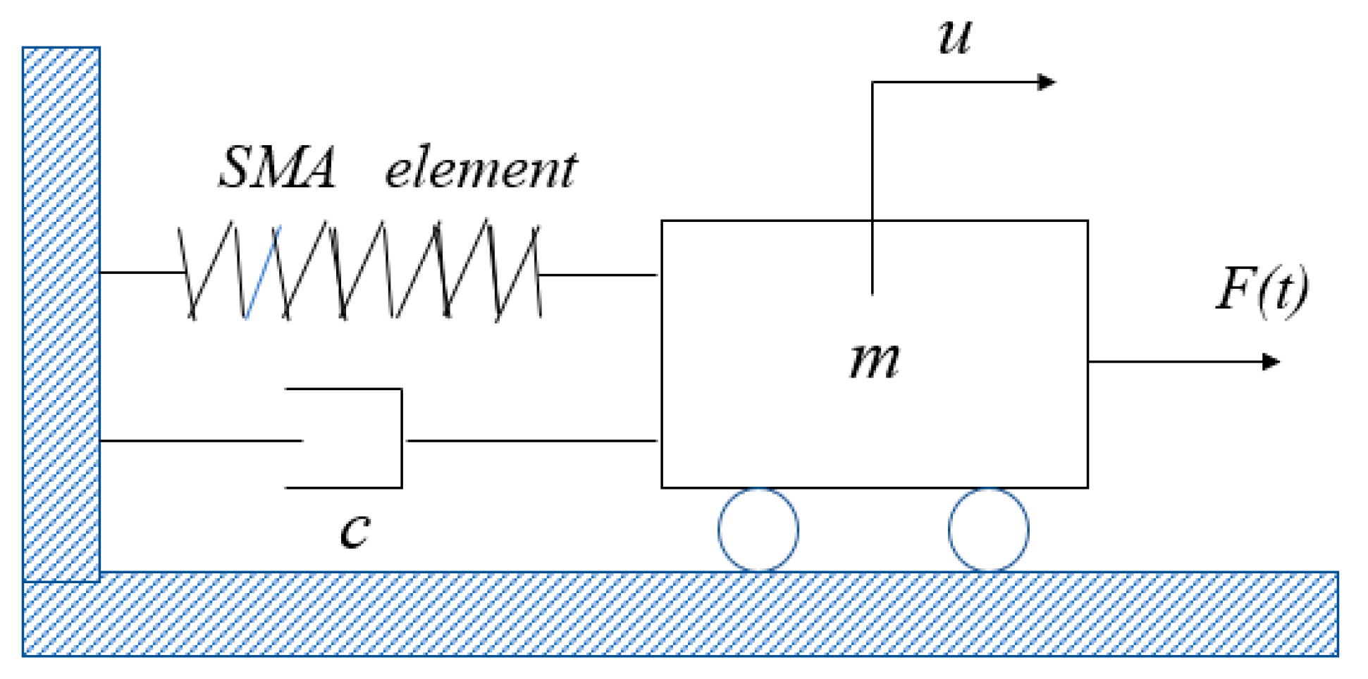
Now, we consider a SDOF SMA oscillator model as shown in Figure 1, where a mass $m$ is connected to a rigid support through of a viscous damping with coefficient $c$ and a shape memory element, and the mass block is subjected to an external force $F\left(t\right)$.

By Newton’s second law, the motion equation of vibration of the system can be expressed as

$$m\ddot{u}+c\dot{u}+\overline{a_1}\left(T-T_M\right)u-\overline{a_2}{u}^3+\overline{a_3}{u}^5=-m\ddot{\overline{u_b}} ,$$

(5)

where $u$ represents the displacement of the mass $m$, the dot denotes a derivative with respect to the time $t$, and $\ddot{\overline{u_b}}$ denotes the base acceleration.

In order to obtain a dimensionless equation of motion, we introduced the following nondimensional transformations

$$\begin{gathered} x=\frac{u}{L};x_b=\frac{\overline{u_b}}{L}, \tau ={\omega }_{0}t;\theta =\frac{T}{T_M};\alpha =\theta -1;\beta =-\frac{a_{2}A}{mL{\omega }_0^2}; \\ \gamma =\frac{a_{3}A}{mL{\omega }_0^2};\zeta =\frac{c}{m{\omega }_0};{\omega }_0^2=\frac{a_{1}A{T}_M}{mL}. \end{gathered}$$

(6)

where $x$, $\tau$, $\zeta$, and $\theta$ are the dimensionless displacement, time, damping coefficient, and temperature, respectively. As the SMAs exhibit different properties depending on the temperature $\theta$, we only considered the temperature where the phase is stable in the alloy, that is, $\theta >1$ in the present study.

Then, the dimensionless equation of nonlinear random vibration of the SMA oscillator systems can be rewritten as

$$\ddot{x}+\zeta \dot{x}+\alpha x+\beta x^3+\gamma x^5=-\ddot{x_b}.$$

(7)

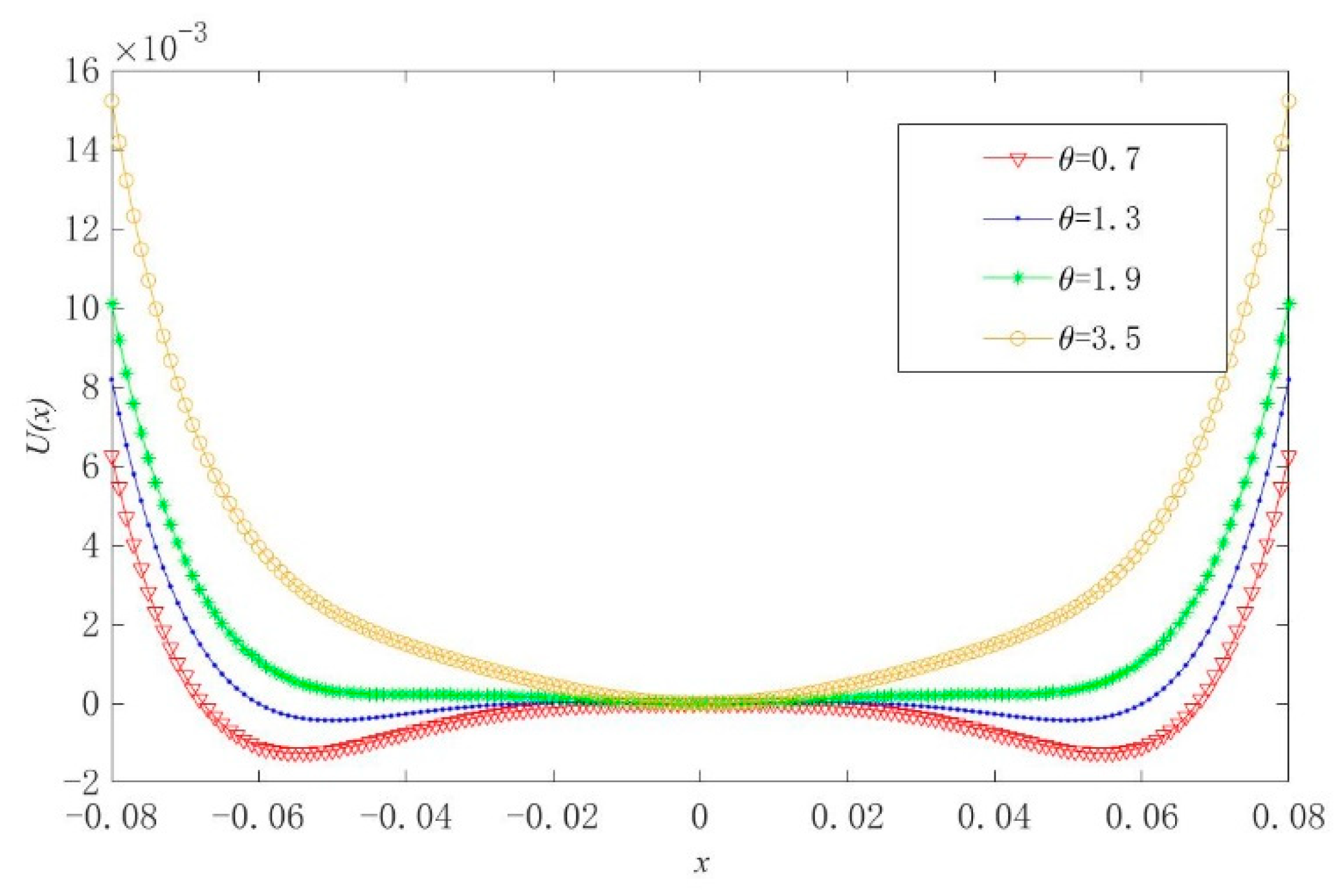
The dimensionless potential function $U\left(x\right)$ of the SMA oscillator can be expressed as the following general form:

$$U\left(x\right)=\frac{1}{2}\alpha x^2+\frac{1}{4}\beta x^4+\frac{1}{6}\gamma x^6.$$

(8)

Depending on parameters of the nonlinear terms $\alpha$, $\beta$, and $\gamma$, the potential function $U\left(x\right)$ has three kinds of different potentials, as shown in Figure 2. According to the activation temperature ${\theta }_A=1.9$, the SMA oscillator can be divided into the following three categories [27]:

A.

$\theta \le 1$ (low temperature). The potential function has two minima and one maximum, that is, three fixed points.

B.

$1<\theta <{\theta }_A$ (medium temperature). The potential function has three stable equilibria and two unstable saddle points. Switching among the three wells or restricted in one of three potential wells depending on the total energy and the initial condition.

C.

$\theta ={\theta }_A$. The potential has three minima.

D.

$\theta >{\theta }_A$ (high temperature). The potential function has only one minimum (potential well).

In the present study, we considered $-\ddot{x_b}=\eta \left(\tau \right)$, where $\eta \left(\tau \right)$ is a random process used to characterize random disturbances of the external environment, which is expressed as follows:

$$\eta \left(\tau \right)=f\cos \left[\mathsf{\Omega }\tau +hW\left(\tau \right)\right],$$

(9)

where $f$ and $\mathsf{\Omega }$ denote the amplitude and the central frequency of the random excitation, respectively; $W\left(\tau \right)$ is the standard Wiener process; and $h\ge 0$ is the noise intensity. Obviously, the random excitation $\eta \left(\tau \right)$ will degenerate into a deterministic periodic force if $h=0$. The corresponding power spectrum density of the random process $\eta \left(\tau \right)$ is given as follows [19,21]:

$$S_{\eta }\left(\omega \right)=\frac{1}{2}\frac{f^2{h}^2\left({\mathsf{\Omega }}^2+{\omega }^2+h^4/4\right)}{{\left({\mathsf{\Omega }}^2-{\omega }^2+h^4/4\right)}^2+{\omega }^2{h}^4},$$

(10)

We uncovered that, when the noise intensity $h$ is small, the spectrum $S_{\eta }\left(\omega \right)$ concentrates on a narrow-band region, which can be regarded as a narrow-band process. In the present paper, only a narrow-band noise case is considered, i.e., the noise intensity $h$ is assumed to be a small parameter.

In this investigation, to realize the theoretical analysis, we assumed that the SMA oscillator has a weak nonlinearity. Hence, a small parameter $0<\epsilon \ll 1$ was introduced to rescale the following parameters as

$$\zeta \to \epsilon \zeta , \beta \to \epsilon \beta ,\gamma \to \epsilon \gamma ,f\to \epsilon f.$$

Thus, the governed equation of the established SMA oscillator model can be rewritten as

$$\ddot{x}+\epsilon \zeta \dot{x}+\alpha x+\epsilon \beta x^3+\epsilon \gamma x^5=\epsilon f\cos \left[\mathsf{\Omega }\tau +hW\left(\tau \right)\right].$$

(11)

3. Theoretical Analysis of the SMA Oscillator Model

In this section, the nonlinear dynamical behaviors are examined for the proposed stochastic SMA oscillator model (11). From Equation (11), we find that the nonlinearity of the system is caused by the constitutive relationship of the SMA material. The dynamic characteristics of the system are also affected by the temperature and the random external excitation, and therefore the nonlinear dynamic behaviors of the system may be complicated.

The multiple-scale method is implemented only for the primary resonance, i.e., the excitation frequency is close to the natural frequency of the SMA oscillator system. Thus, a detuning frequency $\sigma$ is introduced, such that

$${\mathsf{\Omega }}^2=\alpha +\epsilon \sigma .$$

(12)

Then, Equation (11) can be rewritten in the following form:

$$\ddot{x}+\epsilon \zeta \dot{x}+{\mathsf{\Omega }}^{2}x-\epsilon \sigma x+\epsilon \beta x^3+\epsilon \gamma x^5=\epsilon f\cos \left[\mathsf{\Omega }\tau +hW\left(\tau \right)\right].$$

(13)

Introducing fast and slow time scales as follows:

$$T_0=\tau ,T_1=\epsilon \tau ,T_2={\epsilon }^2\tau ,\cdot \cdot \cdot$$

(14)

Using the differential operators

$$D_0=\frac{\partial }{\partial T_0},D_1=\frac{\partial }{\partial T_1},D_2=\frac{\partial }{\partial T_2},\cdot \cdot \cdot$$

(15)

Then, applying the chain rule, we can transform the ordinary derivatives into partial derivatives [26] as

$$\begin{gathered} \frac{d }{d\tau }=D_0+\epsilon D_1+{\epsilon }^2{D}_2+\cdot \cdot \cdot , \\ \frac{d^2 }{d{\tau }^2}=D_0^2+2\epsilon D_0{D}_1+{\epsilon }^2(D_1^2+2D_0{D}_2)+\cdot \cdot \cdot . \end{gathered}$$

(16)

According to the standard procedure of the multiple-scale method, the approximate analytic solutions of the SMA oscillator systems (13) can be expressed in the following form:

$$x=x_0\left(T_0,T_1\right)+\epsilon x_1\left(T_0,T_1\right)+\cdot \cdot \cdot$$

(17)

Substituting Equations (16) and (17) into Equation (13) and separating the term of the yielded equation by the power of $\epsilon$, we derive the following equations

$$O\left({\epsilon }^0\right):D_0^2{x}_0+{\mathsf{\Omega }}^2{x}_0=0,$$

(18)

$$\begin{gathered} O\left({\epsilon }^1\right):D_0^2{x}_1+{\mathsf{\Omega }}^2{x}_1=-2D_0{D}_1{x}_0-\zeta D_0{x}_0+\sigma x_0-\beta x_0^3-\gamma x_0^5 \\ +f\cos \left[\mathsf{\Omega }\tau +hW\left(\tau \right)\right], \end{gathered}$$

(19)

The general solutions of Equation (18) can be expressed as

$$x_0\left(T_0,T_1\right)=A\left(T_1\right)e^{i\mathsf{\Omega }{T}_0}+c.c. ,$$

(20)

where $c.c.$ denotes the complex conjugate of the preceding terms.

Substituting Equation (20) into Equation (19), we arrive at

$$\begin{gathered} D_0^2{x}_1+{\mathsf{\Omega }}^2{x}_1=-\left(2i\mathsf{\Omega }{D}_{1}A+i\zeta \mathsf{\Omega }A-\sigma A+3\beta A^2\overline{A}+10\gamma A^3{\overline{A}}^2\right)e^{i\mathsf{\Omega }{T}_0} \\ -\left(\beta A^3+ 5\gamma A^4\overline{A}\right)e^{3i\mathsf{\Omega }{T}_0}-\gamma A^5{e}^{5i\mathsf{\Omega }{T}_0} \\ +f\cos \left[\mathsf{\Omega }{T}_0+\overline{h}W\left(T_1\right)\right]+c.c. , \end{gathered}$$

(21)

where $D_{1}A$ stands for the derivative with the respect to the slow time scale $T_1$, $\overline{A}$ means the conjugate of $A$, and

$$hW\left(\tau \right)=hW\left(T_0\right)=hW\left(\frac{T_1}{\epsilon }\right)=\frac{h}{\sqrt{\epsilon }}W\left(T_1\right):=\overline{h}W\left(T_1\right).$$

(22)

Substituting Equation (17) into Equation (21) and eliminating the secular terms, we yield

$$-2i\mathsf{\Omega }{D}_{1}A-i\zeta \mathsf{\Omega }A+\sigma A-3\beta A^2\overline{A}-10\gamma A^3{\overline{A}}^2+\frac{1}{2}f{e}^{iW\left(T_1\right)}=0.$$

(23)

The complex amplitude in the polar form is expressed as follows:

$$A\left(T_1\right)=\frac{1}{2}a\left(T_1\right)e^{i\phi \left(T_1\right)},\overline{A}\left(T_1\right)=\frac{1}{2}a\left(T_1\right)e^{-i\phi \left(T_1\right)}.$$

Then, we can obtain

$$i\mathsf{\Omega }{D}_{1}a-\mathsf{\Omega }a{D}_1\phi +\frac{1}{2}i\zeta \mathsf{\Omega }a-\frac{1}{2}\sigma a+\frac{3}{8}\beta a^3+\frac{5}{16}\gamma a^5-\frac{1}{2}f{e}^{i\left[\overline{h}W\left(T_1\right)-\phi \right]}=0.$$

(24)

For convenience, let

$$\varphi =\overline{h}W\left(T_1\right)-\phi ,$$

(25)

$$i\mathsf{\Omega }{D}_{1}a-\mathsf{\Omega }a{D}_1\phi +\frac{1}{2}i\zeta \mathsf{\Omega }a-\frac{1}{2}\sigma a+\frac{3}{8}\beta a^3+\frac{5}{16}\gamma a^5-\frac{1}{2}f{e}^{i\varphi }=0.$$

(26)

Separating real and imaginary parts for the Equation (26), we deduce two so-called modulation equations to

$$\{\begin{array}{c}{D}_{1}a=\frac{1}{2\mathsf{\Omega }}f\sin \varphi -\frac{1}{2}\zeta a,\\ a{D}_1\phi =-\frac{1}{2\mathsf{\Omega }}a\sigma +\frac{3}{8\mathsf{\Omega }}\beta a^3+\frac{5}{16\mathsf{\Omega }}\gamma a^5-\frac{1}{2\mathsf{\Omega }}f\cos \varphi .\end{array}$$

(27)

Due to $D_1\varphi =\overline{h}{D}_{1}W\left(T_1\right)-D_1\phi$, that is, $a{D}_1\varphi =a\overline{h}{D}_{1}W\left(T_1\right)-a{D}_1\phi$, Equation (27) can be rewritten as

$$\{\begin{array}{c}{D}_{1}a=\frac{1}{2\mathsf{\Omega }}f\sin \varphi -\frac{1}{2}\zeta a,\\ a{D}_1\varphi =a\overline{h}{D}_{1}W\left(T_1\right)+\frac{1}{2\mathsf{\Omega }}a\sigma -\frac{3}{8\mathsf{\Omega }}\beta a^3-\frac{5}{16\mathsf{\Omega }}\gamma a^5+\frac{1}{2\mathsf{\Omega }}f\cos \varphi .\end{array}$$

(28)

Accordingly, the amplitude $a$ and the phase $\phi$ can be calculated from Equation (28). Then the first-order approximate solution of the SMA oscillator model (13) is formulated as

$$x=a\cos \left(\mathsf{\Omega }\tau +\phi \right)+O\left(\epsilon \right),$$

(29)

where $O\left(\epsilon \right)$ represents the high-order terms of small parameter $\epsilon$.

Next, we concentrate on the steady-state solutions of Equation (13).

Case 1: The deterministic case, i.e., the intensity of noise $\overline{h}=0$.

Equation (13) is reduced to a deterministic differential equation with harmonic excitation in this case. Considering the steady-state situation, i.e., $D_{1}a=D_1\varphi =0$, one obtains

$$\{\begin{array}{c}\frac{1}{2\mathsf{\Omega }}f\sin \varphi -\frac{1}{2}\zeta a=0,\\ \frac{1}{2\mathsf{\Omega }}a\sigma -\frac{3}{8\mathsf{\Omega }}\beta a^3-\frac{5}{16\mathsf{\Omega }}\gamma a^5+\frac{1}{2\mathsf{\Omega }}f\cos \varphi =0.\end{array}$$

(30)

Then, according to ${\sin }^2\varphi +{\cos }^2\varphi =1$, we obtain the following frequency–amplitude equation

$$f^2={\left(\zeta \mathsf{\Omega }a\right)}^2+{\left(-a\sigma +\frac{3}{4}\beta a^3+\frac{5}{8}\gamma a^5\right)}^2.$$

(31)

Case 2: The stochastic case, i.e., the intensity of noise $\overline{h}\ne 0$.

When $\overline{h}\ne 0$, the effects of the noise have to be considered. The solution of Equation (28) cannot be given analytically, and therefore a perturbation technique is applied here. We suppose that

$$a=a_0+a_1,\varphi ={\varphi }_0+{\varphi }_1,$$

(32)

where $a_0$ and ${\varphi }_0$ are the solutions of the deterministic case, and $a_1$ and ${\varphi }_1$ are small disturbances under the deterministic situations mentioned above, which can be addressed as small parameters. Substituting Equations (30) and (32) into Equation (28) and eliminating the high-order small items, we obtain

$$\{\begin{array}{c}{D}_1{a}_1=\frac{1}{2\mathsf{\Omega }}f{\varphi }_1\cos {\varphi }_0-\frac{1}{2}\zeta a_1,\\ D_1{\varphi }_1=\overline{h}{D}_{1}W\left(T_1\right)-\frac{3}{4\mathsf{\Omega }}\beta a_0{a}_1-\frac{5}{4\mathsf{\Omega }}\gamma a_0^3{a}_1\\ -\frac{1}{2\mathsf{\Omega }{a}_0}f{\varphi }_1\sin {\varphi }_0-\frac{1}{2\mathsf{\Omega }{a}_0{}^2}f{a}_1\cos {\varphi }_0.\end{array}$$

(33)

We transformed Equation (33) into $\mathrm{It}ô$ stochastic differential equation as follows:

$$\{\begin{array}{c}d{a}_1=(\frac{1}{2\mathsf{\Omega }}f{\varphi }_1\cos {\varphi }_0-\frac{1}{2}\zeta a_1)d{T}_1,\\ d{\varphi }_1=(-\frac{3}{4\mathsf{\Omega }}\beta a_0{a}_1-\frac{5}{4\mathsf{\Omega }}\gamma a_0{}^3{a}_1-\frac{1}{2\mathsf{\Omega }{a}_0}f{\varphi }_1\sin {\varphi }_0\\ -\frac{1}{2\mathsf{\Omega }{a}_0{}^2}f{a}_1\cos {\varphi }_0)d{T}_1+\overline{h}dW\left(T_1\right).\end{array}$$

(34)

Under the steady-state situation, the moment equations should satisfy

$$\frac{dE\left(a_1\right)}{d{T}_1}=\frac{dE\left({\varphi }_1\right)}{d{T}_1}=\frac{dE\left(a_1^2\right)}{d{T}_1}=\frac{dE\left({\varphi }_1^2\right)}{d{T}_1}=\frac{dE\left(a_1{\varphi }_1\right)}{d{T}_1}=0.$$

(35)

Here, $E(·)$ is the mathematical expectation operator. Then, first- and second-order steady-state moments of the amplitude $a_1$ can be obtained as follows:

$$\begin{gathered} E(a_1)=0, \\ E\left(a_1^2\right)=\frac{{\overline{h}}^2{M}_2^2}{M_1{M}_2{N}_1+M_1{N}_2^2+M_1^2{N}_2+N_1{N}_2{M}_2}, \end{gathered}$$

(36)

where

$$\begin{gathered} M_1=\zeta ,M_2=\frac{1}{\mathsf{\Omega }}f\cos {\varphi }_0, \\ {N}_1=\frac{3}{2\mathsf{\Omega }}\beta a_0+\frac{5}{2\mathsf{\Omega }}\gamma a_0{}^3+\frac{1}{\mathsf{\Omega }{a}_0{}^2}f\cos {\varphi }_0,N_2=\frac{1}{\mathsf{\Omega }{a}_0}f\sin {\varphi }_0. \end{gathered}$$

(37)

Thus, the first- and second-order steady-state moments of the steady-state solution of Equation (28) are deduced to

$$\{\begin{array}{c}E\left(a\right)=a_0+E(a_1)=a_0,\\ E\left(a^2\right)=a_0^2+E\left(a_1^2\right)=a_0^2+\frac{{\overline{h}}^2{M}_2^2}{M_1{M}_2{N}_1+M_1{N}_2^2+M_1^2{N}_2+N_1{N}_2{M}_2}.\end{array}$$

(38)

According to the literature [16], we can find that if $0<\theta \le 1$, martensite is stable; if $1<\theta <{\theta }_A$, both phases exist; if $\theta >{\theta }_A$, austenite is stable. The unique mechanical properties of SMA are derived from the phase transition, which can be induced by the change of temperature. Therefore, the temperature $\theta$ is an extremely important parameter for the SMA systems. In the next section, effects of the temperature $\theta$ are examined in detail on the nonlinear behaviors of the proposed SMA oscillator model.

4. Numerical Verification

To verify the effectiveness of the obtained analytical results, we compared the differences between the numerical results and the approximately analytical ones through numerical simulations at different temperatures $\theta$ in the next step.

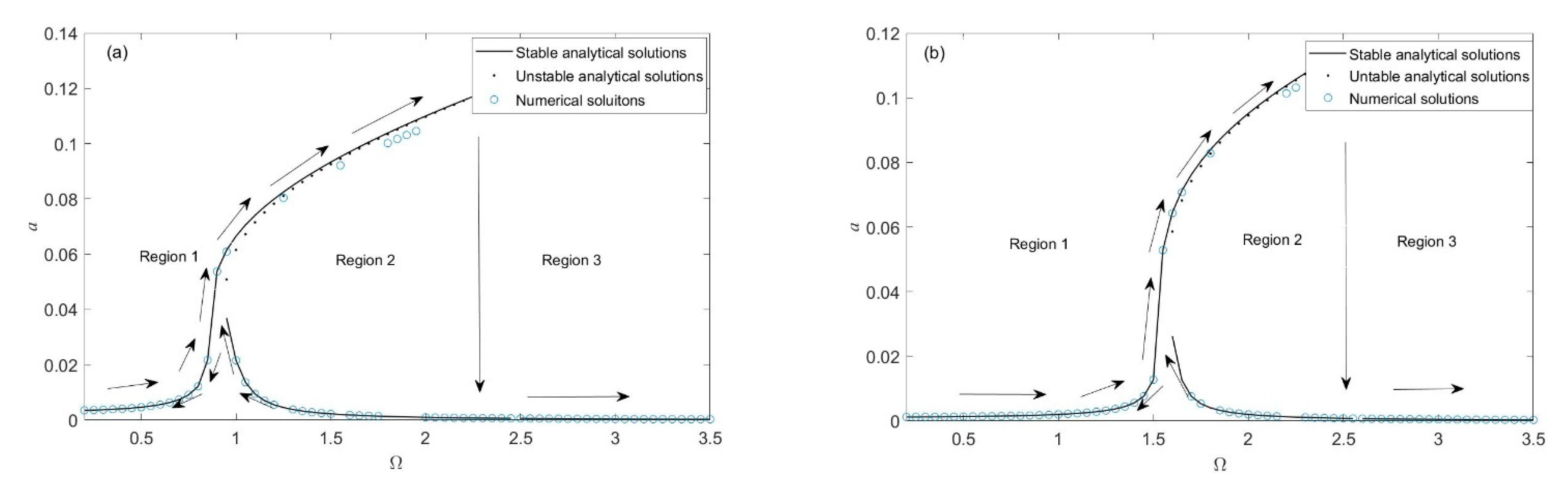
In Figure 3, we consider the deterministic case, namely, $\overline{h}=0$; here, we select the temperature $\theta =1.9$ and $\theta =3.5$ for the sake of verification. Clearly, the approximately analytical results are in good agreement with the numerical simulation results, and multi-value response area can be observed. In this area, the steady-state responses of the SMA oscillator system have two possible states (i.e., bistable behavior), which strongly depend on the initial conditions of the system. At the same time, we found that there is a jump phenomenon in the SMA oscillation system. In Figure 3a, when both martensite and austenite exist, as indicated by the arrow, when the frequency reached a certain critical value from Region 2 to Region 3 with the increase of the external excitation frequency $\mathsf{\Omega }$, a sudden jump occurred in the frequency–amplitude response. If the external excitation frequency $\mathsf{\Omega }$ gradually decreased, when the frequency value $\mathsf{\Omega }$ varied from Region 2 to Region 1, a similarly sudden jump can be observed. This phenomenon can be called a bifurcation, essentially a change in the nature of the solution. The same jump phenomenon occurred when the austenite was stable, that is, $\theta =3.5$.

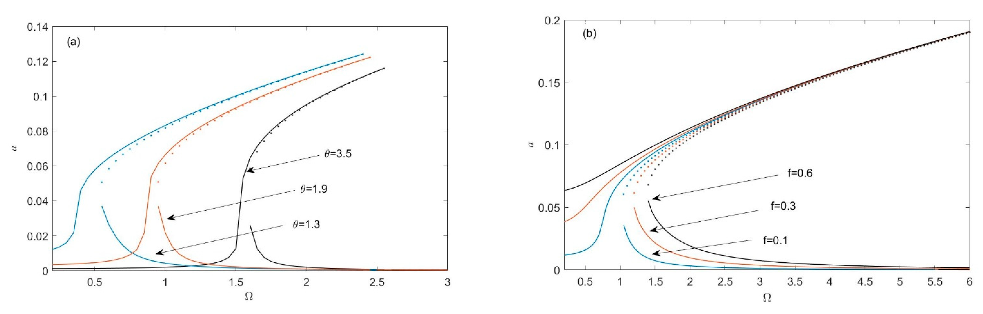
For the deterministic case, we also considered the influences of the temperature $\theta$ and the amplitude $f$ of the external excitation on the amplitude of the SMA system (11). In Figure 4, we find that as the temperature $\theta$ increased, the multi-value response area shifted to the right and the area became smaller. In contrast, the amplitude of the system response and multiple-value response area will become larger with the increase of $f$.

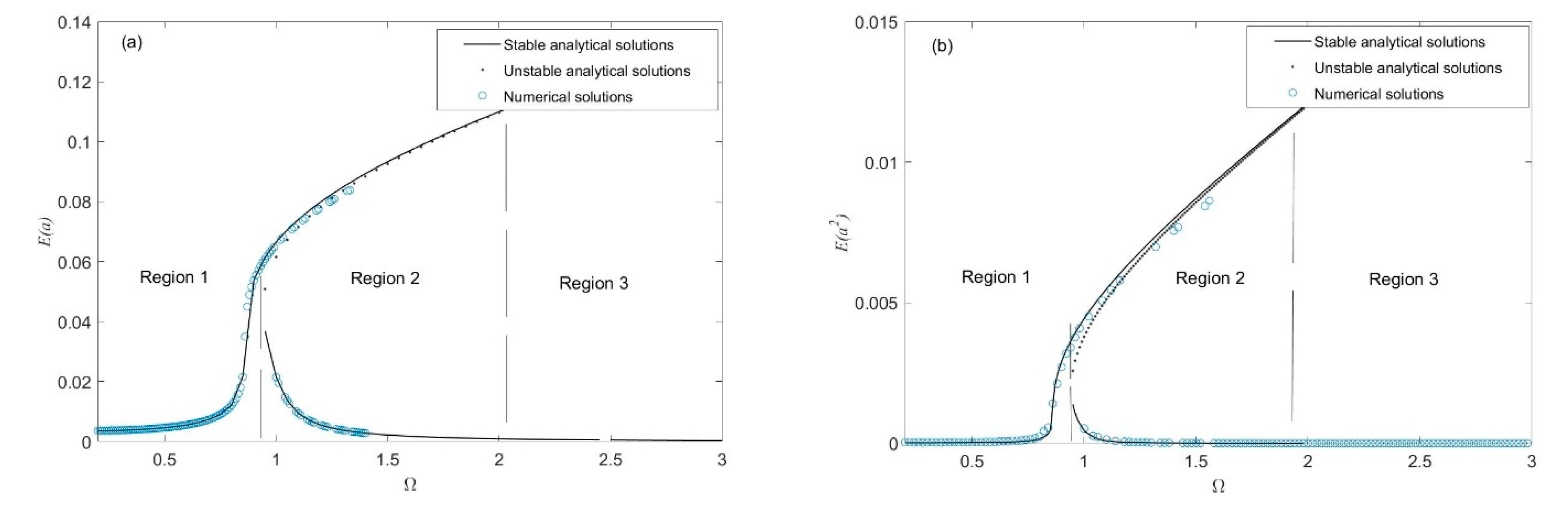
Subsequently, the stochastic case is considered in Figure 5. It intuitively shows that both the analytical first- and second-order moments of the amplitude a coincided well with the numerical results. We can also find that there were still jump phenomena with the increasing or decreasing of the frequency $\mathsf{\Omega }$ in the random situations.

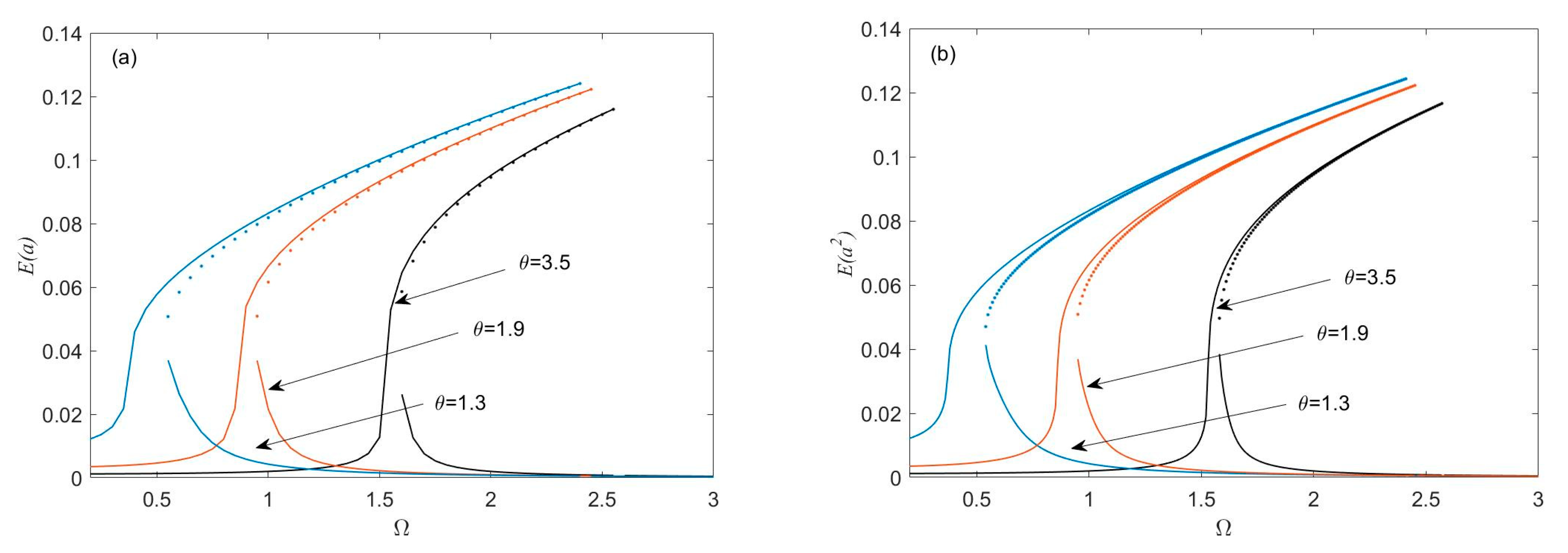
As can be seen from Figure 6, the first-order moment response curve shifted to the right with the temperature $\theta$ increases, and the second-order moment response was the same. For the temperature parameter $\theta$, as the frequency $\mathsf{\Omega }$ increased and reached a certain threshold, the amplitude of the system gradually increased, and the solution of the system changed at the same time, which indicates that the frequency $\mathsf{\Omega }$ can be regarded as a bifurcation parameter of the system. In addition to the above, we can see from Figure 6a, as the temperature parameter $\theta$ increased, we found that the frequency of bifurcation point gradually increased, namely, the lower the temperature, the earlier bifurcation will occur. This phenomenon is the same in Figure 6b.

In fact, a reversed phenomenon can be found from Figure 3, Figure 4, Figure 5 and Figure 6. As is shown in Figure 5, we can see that there was only one stable solution in Region 1, then two stable solutions and one unstable solution came later in Region 2, and finally it again came to one stable solution in Region 3. Thus, the switch phenomenon will occur when the frequency $\mathsf{\Omega }$ changes from Region 2 to Region 1 and from Region 2 to Region 3. This phenomenon can be regarded as bifurcation, that is to say, in this bistable area, the noise may cause stochastic switching in the SMA system, and then we consider the influence of random noise in the next.

Here, the stochastic switch behaviors of the SMA oscillator system (11) subject to narrow-band random excitation were investigated to observe the effects of the random noise. Monte Carlo simulation was used to demonstrate the steady-state probability density functions (PDFs) and the responses. From here, we consider the effects of the noise intensity $h$ on the random responses of the SMA oscillator system (13).

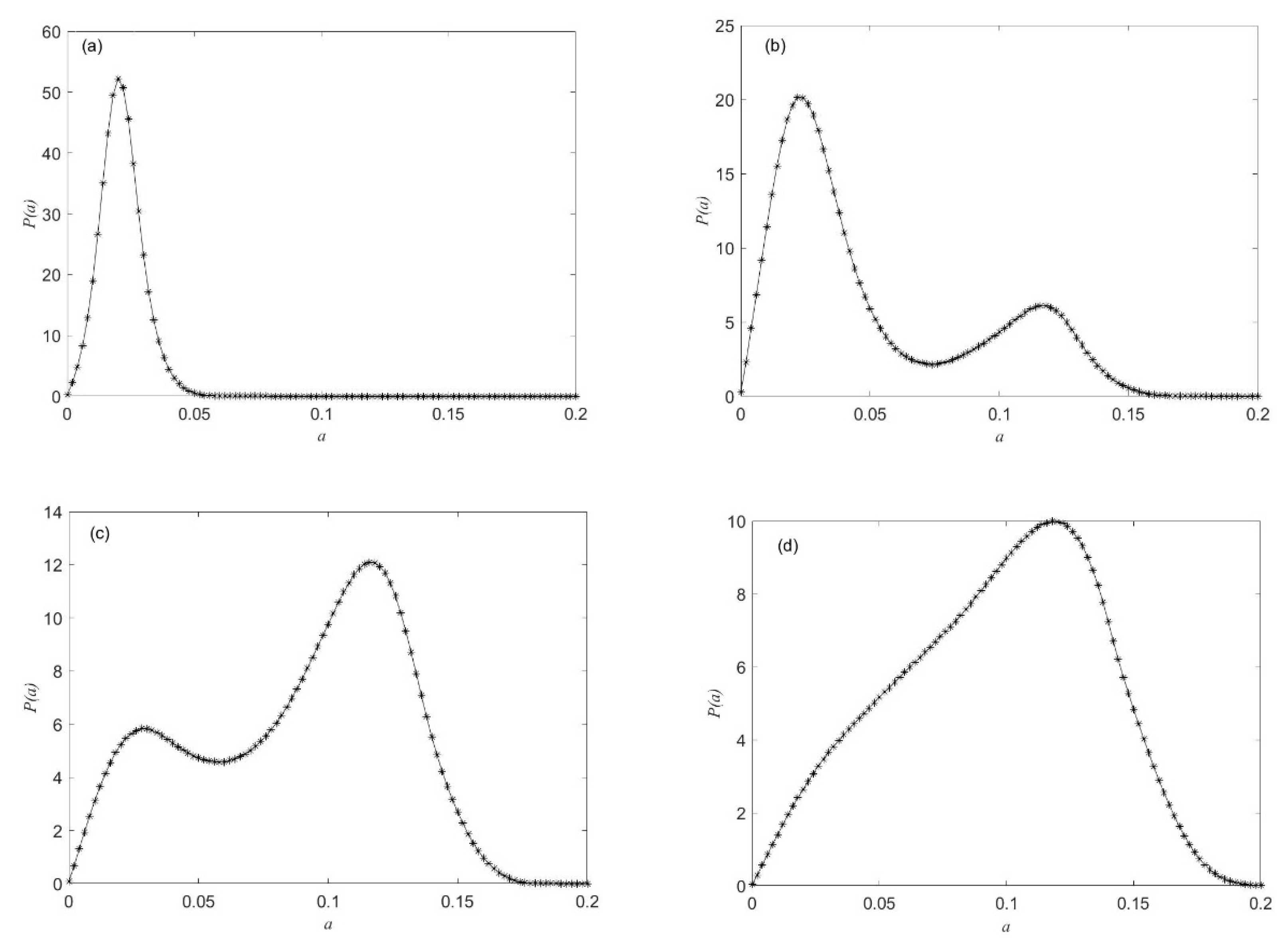
Figure 7 presents the effects of the noise intensity $h$ on the steady-state PDF $P\left(a\right)$ of the amplitude $a\left(\tau \right)=\sqrt{x^2\left(\tau \right)+{\left[\dot{x}\left(\tau \right)/\mathsf{\Omega }\right]}^2}$, with the fixed system parameters $f=0.6$, $\mathsf{\Omega }=2.0$. As shown in Figure 7a–d, when adding a small noise, we can see that the noise will cause the appearance of a peak change in the steady-state PDF. The switch of the SMA oscillator model under random fluctuation is essentially a transition of the dynamic responses from one probable state to another one, which will be intuitively visualized in the following parts through time history responses. Thus, we only observed one peak lying in the low-amplitude oscillation state in Figure 7a. However, double peaks can be induced in the steady-state PDFs with the increase of the noise intensity gradually. One can imagine from the PDFs that the steady-state response of the proposed SMA model contains two kinds of probable motions, that is, random vibrations with high-amplitude or low-amplitude, which means the stochastic switch occurs. Furthermore, when the noise intensity is large enough, the steady-state PDFs tend towards one peak again, as shown in Figure 7d.

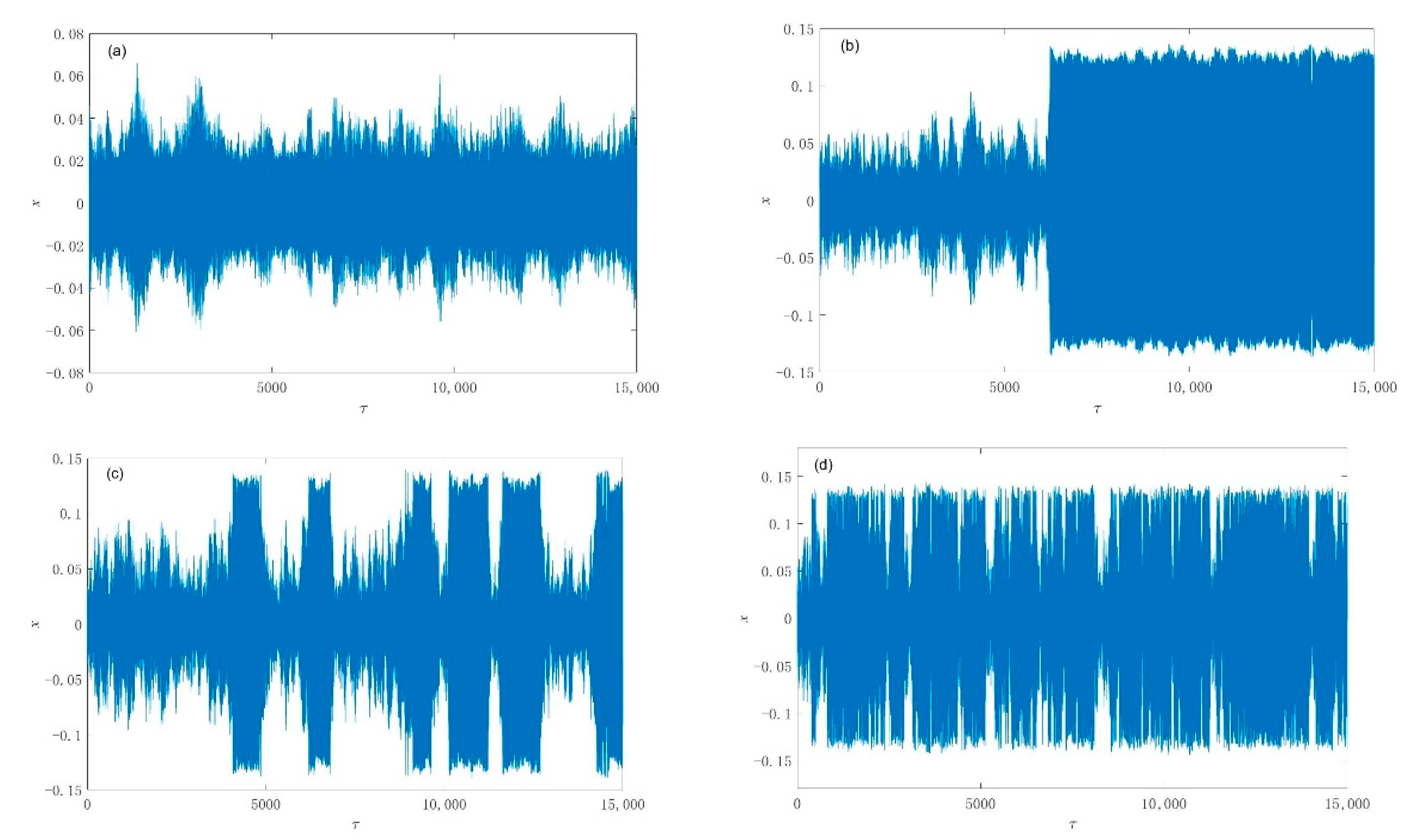
To further intuitively exhibit the switch phenomena shown in Figure 7, we plotted a number of typical time history diagrams in Figure 8. As shown in Figure 8, the system response was only subjected to minor disturbances when the noise intensity was small, and a switch phenomenon was not observed, whereafter, an obvious switch phenomenon from the low-amplitude oscillation state to the high-amplitude state was found, as shown in Figure 8b–d. In other words, with the increase of the noise intensity gradually, the stochastic switch phenomenon will occur increasingly more frequently. Therefore, we conclude that the noise is able to lead to a stochastic switch that can be viewed as the stochastic P-bifurcation due to the change of peak number of the steady-state PDFs. Those stochastic switches will damage the SMA material and even affect the safety of the SMA oscillator.

5. Conclusions

In this paper, we explored the nonlinear dynamical responses of a SMA oscillator model with a narrow-band random excitation. The multiple-scale method was employed to achieve the theoretical analysis of the proposed stochastic SMA oscillator system. We uncovered the fact that the obtained analytical solutions coincided perfectly with the numerical ones for both the deterministic and stochastic cases. The stochastic switch and bifurcation were observed from the stationary PDFs and the time history responses with the change of the noise intensity. The results show that the PDFs changed from one peak to double and then gradually to one peak again with the increase of the noise intensity, which indicates that the noise intensity has a great influence on the properties of SMA materials and can lead to stochastic switch and bifurcation. We also explained the phenomena of stochastic switch and bifurcation via the time history responses at different noise intensities.

From the perspective of practical applications, a random disturbance with small intensity will destroy the stable structure of the SMA oscillator system, which causes the original system to produce strong disordered oscillations and operational collapse in a stable state. Therefore, it is of great significance to study the influences of random disturbances on the evolution of the dynamic behaviors of the system for the safe and reliable operation of the SMA oscillation system.

References

- Jani, J.M.; Leary, M.; Subic, A.; Gibson, M.A. A review of shape memory alloy research, applications and opportunities. Mater. Des. 2014, 56, 1078–1113. [Google Scholar] [CrossRef]
- Lagoudas, D.C. Shape Memory Alloys: Modeling and Engineering Applications; Springer: New York, NY, USA, 2008. [Google Scholar]
- Paiva, A.; Savi, M. An overview of constitutive models for shape memory alloys. Math. Probl. Eng. 2006, 2006, 1–30. [Google Scholar] [CrossRef]
- Machado, L.G.; Savi, M.A. Medical applications of shape memory alloys. Braz. J. Med Biol. Res. 2003, 36, 683–691. [Google Scholar] [CrossRef]
- Chau, E.T.F.; Friend, C.M.; Allen, D.M.; Hora, J.; Webster, J.R. A technical and economic appraisal of shape memory alloys for aerospace applications. Mater. Sci. Eng. A 2006, 438–440, 589–592. [Google Scholar] [CrossRef]
- Denoyer, K.K.; Scott, E.R.; Rory, N.R. Advanced smart structures flight experiments for precision spacecraft. Acta Astronaut. 2000, 47, 389–397. [Google Scholar] [CrossRef]
- Toi, Y.; Lee, J.-B.; Taya, M. Finite element analysis of superelastic, large deformation behavior of shape memory alloy helical springs. Comput. Struct. 2004, 82, 1685–1693. [Google Scholar] [CrossRef]
- Sreekanth, M.; Mathew, A.T.; Vijayakumar, R. A novel model-based approach for resistance estimation using rise time and sensorless position control of sub-millimetre shape memory alloy helical spring actuator. J. Intell. Mater. Syst. Struct. 2018, 29, 1050–1064. [Google Scholar] [CrossRef]
- Machado, L.G.; Savi, M.A.; Pacheco, P.M.C. Nonlinear dynamics and chaos in coupled shape memory oscillators. Int. J. Solids Struct. 2000, 40, 5139–5156. [Google Scholar] [CrossRef]
- Lacarbonara, W.; Bernardini, D.; Vestroni, F. Periodic and nonperiodic responses of shape-memory oscillators. Int. J. Solids Struct. 2004, 41, 1209–1234. [Google Scholar] [CrossRef]
- Aline, S.; Marcel, V.S.; Marcelo, A.; Wallacw, M. Controlling a shape memory alloy two-bar truss using delayed feedback method. Int. J. Struct. Stab. Dyn. 2014, 14, 1440032. [Google Scholar]
- Shang, Z.J.; Wang, Z.M. Nonlinear Forced Vibration for Shape Memory Alloy Spring Oscillator. Adv. Mater. Res. 2011, 250–253, 3958–3964. [Google Scholar] [CrossRef]
- Spanos, P.D.; Cacciola, P.; Redhorse, J. Random Vibration of SMA Systems via Preisach Formalism. Nonlinear Dyn. 2004, 36, 405–419. [Google Scholar] [CrossRef]
- Dobson, S.; Noori, M.; Hou, Z.; Dimentbetg, M.; Baber, T. Modeling and random vibration analysis of SDOF systems with asymmetric hysteresis. Int. J. Non-Linear Mech. 1997, 32, 669–680. [Google Scholar] [CrossRef]
- Yan, X.; Nie, J. Response of SMA superelastic systems under random excitation. J. Sound Vib. 2000, 238, 893–901. [Google Scholar] [CrossRef]
- Yue, X.L.; Xiang, Y.L.; Xu, Y.; Zhang, Y. Global dynamics of the dry friction oscillator with shape memory alloy. Arch. Appl. Mech. 2020, 90, 2681–2692. [Google Scholar] [CrossRef]
- Yue, X.L.; Xiang, Y.L.; Zhang, Y.; Xu, Y. Global analysis of stochastic bifurcation in shape memory alloy supporter with the extended composite cell coordinate system method. Interdiscip. J. Nonlinear Sci. 2021, 31, 013133. [Google Scholar] [CrossRef]
- Rajan, S.; Davies, H.G. Multiple time scaling of the response of a Duffing oscillator to narrow-band random excitation. J. Sound Vib. 1988, 123, 497–506. [Google Scholar] [CrossRef]
- Rong, H.W.; Xu, W.; Fang, T. Principal response of Duffing oscillator to combined deterministic and narrow-band random parametric excitation. J. Sound Vib. 1998, 210, 483–515. [Google Scholar] [CrossRef]
- Rong, H.W.; Xu, W.; Wang, X.D.; Meng, G.; Fang, T. Response statistics of two-degree-of-freedom nonlinear system to narrow-band random excitation. Int. J. Non-Linear Mech. 2002, 37, 1017–1028. [Google Scholar]
- Rong, H.W.; Xu, W.; Wang, X.D.; Meng, G.; Fang, T. Principal response of Van der Pol–Duffing oscillator under combined deterministic and random parametric excitation. Appl. Math. Mech. 2002, 23, 299–310. [Google Scholar]
- Liu, D.; Xu, W.; Xu, Y. Dynamic responses of axially moving viscoelastic beam under a randomly disordered periodic excitation. J. Sound Vib. 2012, 331, 4045–4056. [Google Scholar] [CrossRef]
- Xu, Y.; Li, Y.G.; Liu, D.; Jia, W.T.; Huang, H. Responses of Duffing oscillator with fractional damping and random phase. Nonlinear Dyn. 2013, 74, 745–753. [Google Scholar] [CrossRef]
- Xu, Y.; Li, Y.G.; Liu, D. Response of fractional oscillators with viscoelastic term under random excitation. J. Comput. Nonlinear Dyn. 2014, 9, 031015. [Google Scholar] [CrossRef]
- Liu, Q.; Xu, Y.; Kurths, J. Bistability and stochastic jumps in an airfoil system with viscoelastic material property and random fluctuations. Commun. Nonlinear Sci. Numer. Simul. 2020, 84, 105184. [Google Scholar] [CrossRef]
- Falk, F. Model free-energy, mechanics and thermodynamics of shape memory alloys. Acta Metall. 1980, 28, 1773–1780. [Google Scholar] [CrossRef]
- Weremczuk, A.; Rekas, J.; Rusinek, R. Low- and high- temperature primary resonance in shape memory oscillator observed by multiple time scales and harmonic balance method. J. Comput. Nonlinear Dyn. 2019, 14, 11002. [Google Scholar] [CrossRef]
Figure 1.
Stochastic dynamic model of shape memory alloys oscillator.
Figure 2.
Potential function of the SMA oscillator system (7) for various relative temperatures with the system parameters: , , .
Figure 3.
Frequency–amplitude response of the SMA oscillator system (11): , , , , . “-” stable analytical solutions, “.”unstable analytical solutions, “o” numerical solutions. (a) ; (b) .
Figure 4.
Frequency–amplitude responses of the SMA oscillator system (11) for different parameters: , ,, . (a) Temperature , ; (b) amplitude of the external excitation, .
Figure 5.
Frequency–amplitude responses of the stochastic SMA oscillator system (11) with the fixed system parameters , , , , , . (a) First-order moment of amplitude ; (b) second-order moment of amplitude : “-” stable analytical solutions, “.”unstable analytical solutions, “o”numerical solutions.
Figure 6.
Frequency–amplitude responses of the stochastic SMA oscillator system (11) for different temperatures : , , , . (a) First-order moment of amplitude ; (b) second-order moment of amplitude .
Figure 7.
The stationary PDFs of amplitude for the original SMA oscillator system (11) with the fixed system parameters , , , , , and different noise intensities (a) ; (b) ; (c) ; (d) . The initial conditions are set to , , corresponding to the low-amplitude oscillation state.
Figure 8.
Time history of the original SMA oscillator system with the same temperature and the fixed system parameters , , , , , , and different noise intensities: (a) ; (b) ; (c) ; (d) . The initial conditions are set to , , corresponding to the low-amplitude oscillation state.
Publisher’s Note: MDPI stays neutral with regard to jurisdictional claims in published maps and institutional affiliations. |
© 2021 by the authors. Licensee MDPI, Basel, Switzerland. This article is an open access article distributed under the terms and conditions of the Creative Commons Attribution (CC BY) license (https://creativecommons.org/licenses/by/4.0/).
Share and Cite
MDPI and ACS Style
Guo, R.; Liu, Q.; Li, J.; Xu, Y. Response Statistics of a Shape Memory Alloy Oscillator with Random Excitation. Appl. Sci. 2021, 11, 10175. https://0-doi-org.brum.beds.ac.uk/10.3390/app112110175
AMA Style
Guo R, Liu Q, Li J, Xu Y. Response Statistics of a Shape Memory Alloy Oscillator with Random Excitation. Applied Sciences. 2021; 11(21):10175. https://0-doi-org.brum.beds.ac.uk/10.3390/app112110175
Chicago/Turabian StyleGuo, Rong, Qi Liu, Junlin Li, and Yong Xu. 2021. "Response Statistics of a Shape Memory Alloy Oscillator with Random Excitation" Applied Sciences 11, no. 21: 10175. https://0-doi-org.brum.beds.ac.uk/10.3390/app112110175
Note that from the first issue of 2016, this journal uses article numbers instead of page numbers. See further details here.