A Study on the Anomaly Detection of Engine Clutch Engagement/Disengagement Using Machine Learning for Transmission Mounted Electric Drive Type Hybrid Electric Vehicles

Abstract

Transmission mounted electric drive type hybrid electric vehicles (HEVs) engage/disengage an engine clutch when EV↔HEV mode transitions occur. If this engine clutch is not adequately engaged or disengaged, driving power is not transmitted correctly. Therefore, it is required to verify whether engine clutch engagement/disengagement operates normally in the vehicle development process. This paper studied machine learning-based methods for detecting anomalies in the engine clutch engagement/disengagement process. We trained the various models based on multi-layer perceptron (MLP), long short-term memory (LSTM), convolutional neural network (CNN), and one-class support vector machine (one-class SVM) with the actual vehicle test data and compared their results. The test results showed the one-class SVM-based models have the highest anomaly detection performance. Additionally, we found that configuring the training architecture to determine normal/anomaly by data instance and conducting one-class classification is proper for detecting anomalies in the target data.

1. Introduction

A transmission mounted electric drive (TMED) type hybrid electric vehicle (HEV) is a parallel hybrid electric vehicle with a structure in which an engine clutch is mounted between an engine and a motor that is connected to a transmission input shaft. In this vehicle structure, the engine clutch is released in EV driving mode, which drives the vehicle only with the motor. The engine clutch is coupled in HEV driving mode, which drives the vehicle with the engine and motor together [1]. According to a power distribution strategy, a hybrid control unit (HCU) drives the vehicle in EV mode or HEV mode [2,3,4,5]. Therefore, EV↔HEV mode transitions can occur when the vehicle is driving, and the engine clutch is engaged or disengaged. If the engine clutch is not adequately engaged or disengaged, power is not transmitted correctly. Thus, it is necessary to verify whether engine clutch engagement/disengagement operates normally in the vehicle development process.

Studies on fault or anomaly detection for vehicle powertrains have been carried out by various approaches. They can be classified by rule-based methods [6,7,8,9,10,11,12], mathematical model-based methods [13,14,15,16,17,18,19,20,21,22,23,24,25,26], and data-driven methods that use signal processing or machine learning [27,28,29,30,31,32,33,34,35,36,37,38,39,40,41,42,43].

First, in the case of using simple rules, Chen proposed a hybrid electric bus’s fault detection method for a HEV by checking the accelerator pedal signal, battery voltage signal range, and logical operation relationship between powertrain components for different driving modes [7]. Ferreira proposed an anomaly score considering activation frequency of diagnostic trouble codes (DTC) by revising binary cross-entropy [10]. When a DTC is activated, the anomaly score is low for frequently activated DTCs and high for infrequently activated DTCs due to different weighting factors for each DTC code. In addition, the fault detection methods with simple logic based on hardware redundancies were proposed [8,11]. Song proposed a fault detection algorithm based on the current flowing through IGBT for an electrical powertrain configuration with hardware redundancies [8]. Pan proposed an internal short circuit fault detection method for lithium-ion battery cells using two current sensors with a symmetrical loop circuit topology [11]. In the case of using mathematical models, the method of using a linear mathematical model of a powertrain component, the method of estimating sensor values using state observers such as Extended Kalman Filters (EKF), Luenberger Observers [15,17,19], and the method based on structural analysis of the target system [18], etc., were proposed. Tabbache proposed a fault-tolerant control strategy for a speed sensor of an EV induction motor using the maximum likelihood voting technique [15]. Roubache conducted fault detection for an EV induction motor using EKF and back-stepping control [17]. Meyer proposed an inter-turn short circuit fault detection and fault degree identification method using moving horizon observer for the Toyota Prius traction motor [19]. In the case of using data-driven techniques, methods using frequency analysis [27,31,34,40], methods using frequency analysis and neural networks together [41], and methods using machine learning such as one-class SVM, Hidden Markov model, and Gaussian mixture model [28,33,36,42], etc., were proposed. Akin proposed a frequency analysis-based fault detection method used at the motor’s zero speed [27]. Källström analyzed powertrain vibrations through time-frequency signal processing to detect a wheel loader clutch fault during the shifting process [31]. Moosavian analyzed the effects of piston scratches on engine vibration using short-time Fourier transform (STFT) and continuous wavelet transform (CWT) [34]. Xu detected engine misfire faults by analyzing the instantaneous angular speed of the engine in the frequency domain [40]. Ewert proposed a fault detection method for motor bearing faults using a machine learning technique based on multi-layer perceptron (MLP), radial basis function (RBF), and self-organizing map (SOM) networks [41]. Nair proposed a machine learning based fault detection method for battery sensors of HEV that used one-class support vector machine (SVM) and k-means clustering together [33]. Kordes detected faults of sensor data in a controller area network (CAN) bus using machine learning with the features by extracting features using cause and effect rules [36]. Jiang conducted fault diagnosis for an EV battery using variational mode decomposition and clustering [42]. In particular, in [44], the authors diagnosed faults of vehicle powertrain by using mathematical models and a neuro-fuzzy network together.

So far, studies aimed at detecting fault or anomalies on vehicle powertrains have been conducted mainly on individual parts such as the motor, battery, and transmission. Little research has been conducted on detecting anomalies in the system operation level of the powertrain control. In [6,22,26], the authors conducted studies to detect anomalies by examining vehicle data trends. In [10,36], the authors detected relatively simple anomalies through DTC signals or a tendency to increase/decrease between data. However, there is a limit to these applications to the verification of complicated control functions. In [32], the authors also studied to detect anomalies by examining vehicle data trends with machine learning. The classifier resulted in relatively low precision, and the precision results were different according to the test data.

Therefore, this paper studied the anomaly detection method for complicated HEV powertrain control functions. In particular, we examined the methods for detecting anomalies in the engine clutch engagement/disengagement process required for EV↔HEV mode transitions, which is a crucial function of TMED type HEVs. We used data-driven methods to make it easy to apply to various vehicle data in the future. Additionally, previous studies’ rule-based methods and mathematical model-based methods have limitations in applying them to target control function. The rule-based techniques are difficult to apply to complex control functions because they use simple rules generally. In addition, it is not easy to construct a mathematical model for the engine clutch engagement/disengagement process. As noted earlier, little research has been conducted on detecting anomalies in the system operation level of the powertrain control. Therefore, we used the basic and most widely used learning architecture. We used multi-layer perceptron (MLP), long short-term memory (LSTM), convolutional neural network (CNN), and one-class support vector machine (one-class SVM) to train the models for anomaly detection and compared the trained models. MLP is the most basic neural network architecture, and CNN and LSTM are the most widely used learning architectures recently. To investigate the performance of the trained model for actual vehicle data, we used real vehicle test data. As a result of the study, we found that the one-class classification method is the most effective.

This paper is organized as follows. Section 2 introduces the structure of TMED type HEVs and the engine clutch engagement/disengagement process in more detail. Section 3 describes the basic data preprocessing for model training and testing, and Section 4 explains the anomaly detection model training methods. Section 5 shows the test results for the trained models, and the conclusions are described in Section 6.

2. Target Vehicle and Data

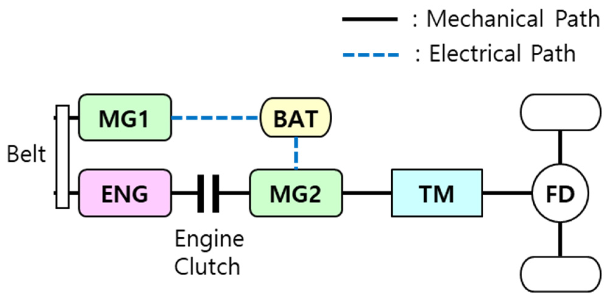
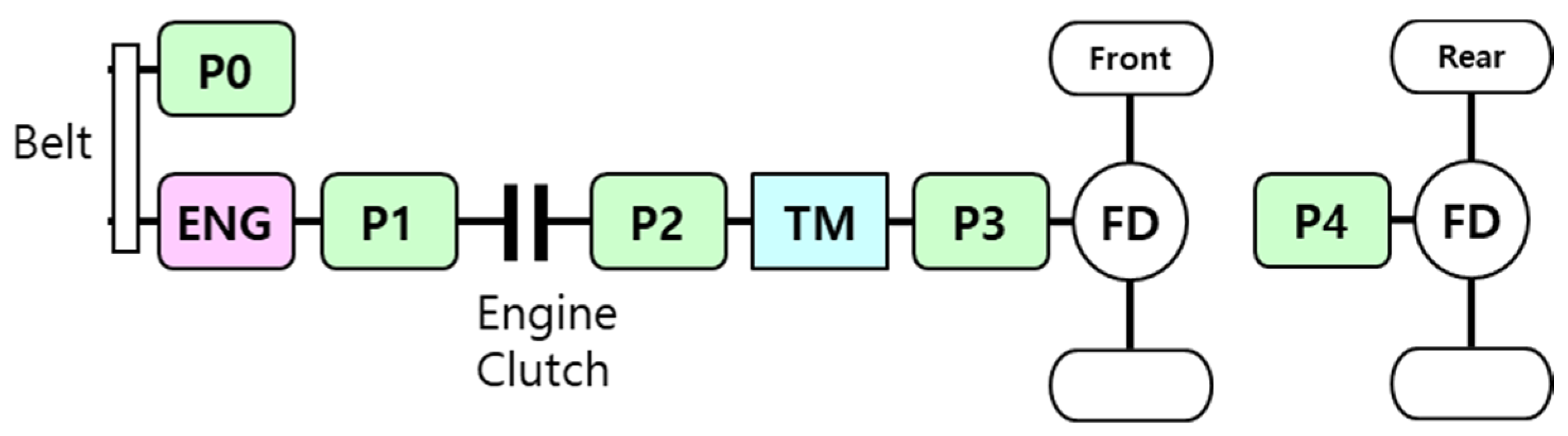
2.1. Target Vehicle

This paper’s target vehicle is a TMED type parallel HEV with the following powertrain structure. This structure is one in which we were able to obtain actual vehicle data. In Figure 1, MG1 represents the BSG (belt-driven starter and generator), MG2 represents the main traction motor, ENG represents the engine, BAT represents the high voltage battery, TM represents the transmission, and FD represents the final drive.

Parallel HEV structures can be classified into P0, P1, P2, P3, and P4 depending on the motor’s position, as shown in Figure 2. In the case of P0 and P1 structures, vehicle electrification can be possible at a low cost, but the fuel efficiency improvement effect is relatively low. In contrast, P2–P4 structures can improve fuel efficiency more, but they are characterized by high system complexity and high construction cost [45]. The target vehicle structure, TMED type HEV, can be seen as a P0 + P2 structure and has the advantages of improving high fuel efficiency using a P2 motor and enabling engine start/generation using the P0 motor.

2.2. Target Data

The TMED type HEV shown in Figure 1 drives the vehicle using MG2 in EV driving mode and drives the vehicle mainly using the engine and MG2 in HEV driving mode. According to a power distribution strategy, an HCU drives the vehicle in EV mode or HEV mode. Therefore EV↔HEV mode transitions can occur when the vehicle is driving. For an HEV→EV mode transition, an HCU gives an EV mode transition command, and then an engine clutch is disengaged with a clutch pressure drop. Additionally, an EV→HEV mode transition is accomplished through the following process [46].

• Cranking an engine using MG1 or MG2;
• Speed synchronization of both sides of the engine clutch (engine and traction motor speed synchronization);
• Engine clutch engagement and transition to HEV mode.

This paper tried to detect anomalies related to this engine clutch engagement/disengagement occurring in EV↔HEV mode transitions.

Table 1. Representative anomalous behaviors in engine clutch engagement/disengagement.

Case	Description
Engine clutch engagement failure	The speed difference between an engine and a motor exceeds a certain level, although an HCU applies an engine clutch command to be fully engaged. (This case is that the engine clutch is not fully engaged as intended. For the target vehicle, as the engine clutch connects the engine and the motor, there should be no speed difference between the engine and the motor when HCU commands the engine clutch as full engagement in normal conditions.)
Engine clutch disengagement failure	The speed difference between an engine and a motor is less than a certain level over a certain time, although an HCU applies an engine clutch command to be released/open and an engine operating mode command to be off for EV mode. (This case is that the engine clutch is not released as intended in EV mode. As a result, the speed difference is small as the engine clutch still connects the engine and the motor. In normal conditions, there should be a speed difference between the engine and the motor because the motor has speed according to the vehicle speed and the engine speed is zero due to the engine off command.)
Clutch pressure command following failure	The difference between a clutch pressure command value and a clutch pressure sensor value exceeds a certain level over a certain time. (This case is that the engine clutch pressure does not follow a command. In normal conditions, the difference between the pressure command and pressure sensor value should be small enough. When the pressure command changes significantly, hydraulic generation delay can slightly increase this difference, but the duration should not be long.)

shows the cases of representative anomalous behavior for such data. An engine clutch engagement failure is the case when the speed difference between an engine and a motor occurs at higher than a certain level, although an HCU applies an engine clutch command to be fully engaged. The engine clutch disengagement failure is the case when the speed difference between an engine and a motor occurs lower than a certain level because the clutch is not released correctly, although an HCU applies an engine clutch command to be released. The clutch pressure command following failure is the case when the clutch pressure does not follow a clutch pressure command from the HCU or TCU (transmission control unit). We collected actual vehicle test data, including the following anomalous behavior cases, and trained the models to detect anomalies with these data.

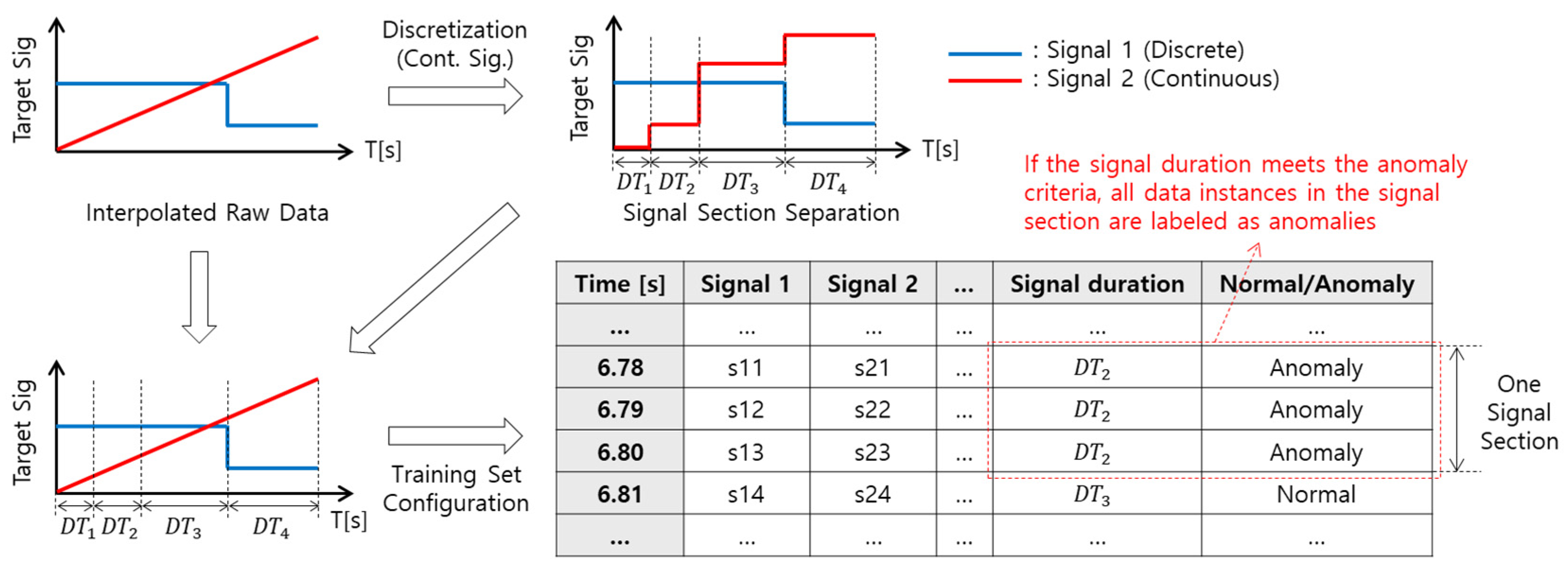
3. Data Preprocessing for Model Training and Test

3.1. Data Interpolation

We used the data acquired through actual vehicle tests to train the models that can detect anomalies. The target data are the signals in the CAN bus related to engine clutch engagement/disengagement. For example, engine speed, clutch status, clutch hydraulic pressure command from the HCU or TCU, etc. Because the target signals are transmitted from various controllers, sampling time and period are slightly different. To synchronize these sampling times, we defined a time vector with a specific period and then conducted linear interpolation of the target signals to this time vector.

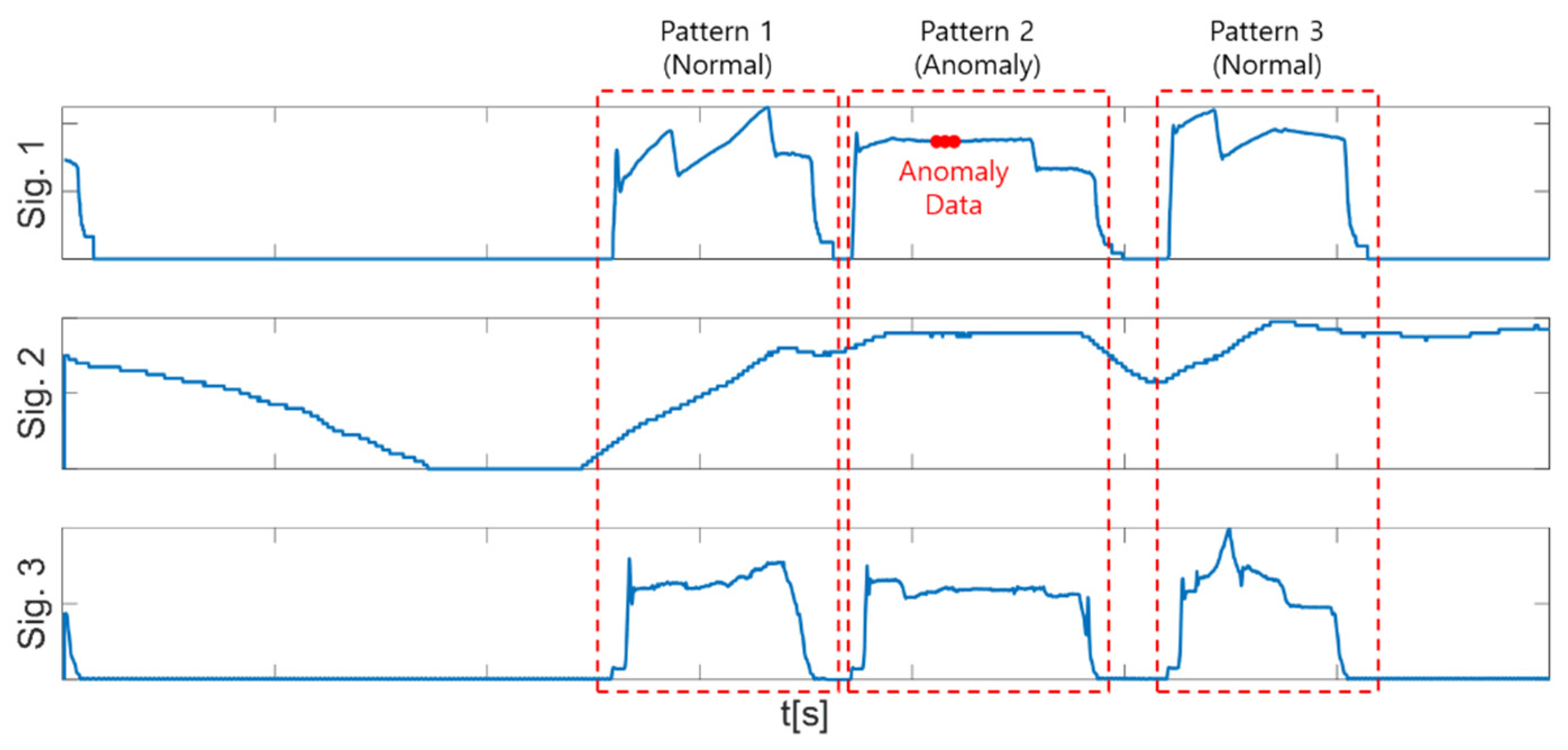
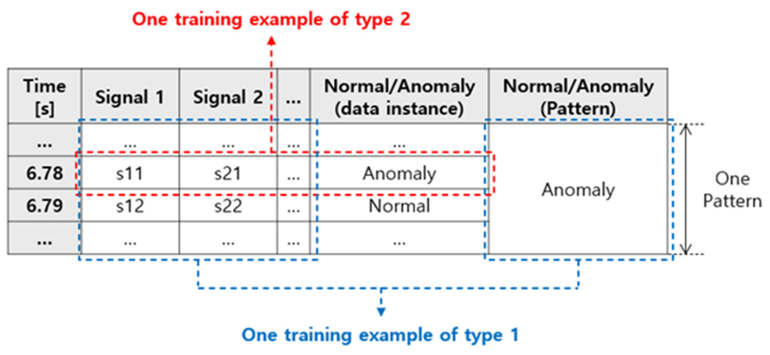
3.2. Target Data Section Extraction (Pattern Extraction)

When driving, an HEV operates in various driving modes according to an HCU’s power distribution strategy. Accordingly, there are cases where an engine clutch is not engaged. For example, an engine clutch is disengaged in EV driving mode, and it is not related to the target situation. To deal with only the related data, we extracted the data from when an engine clutch is engaged to when an engine clutch is disengaged based on the engine clutch control state command signal from the HCU. We then defined one extracted data section as a pattern like a Figure 3. If there are any anomalies in a pattern, the pattern is labeled as an anomaly pattern.

The number of normal/anomaly patterns extracted through this process is shown in

Table 2. The number of engine clutch engagement/disengagement patterns for model training and test (before the copy of anomaly patterns).

	Normal Patterns	Anomaly Patterns
Number of data	1878	25

. We can see that the number of anomaly patterns is much less than the number of normal patterns. This is because developed vehicle control functions are generally first verified through tests such as model-in-the-loop simulation (MILS) and hardware-in-the-loop simulation (HILS) before being applied to actual vehicles. These tests examine unintended behaviors and improve control function’s quality, resulting in fewer anomalous data for controllers and control logic installed in actual vehicles. This normal/anomaly data imbalance is a common phenomenon that occurs not only in vehicles but also in other manufacturing industries. If there are too little anomalous data, it is challenging to learn the characteristics of anomalous data. Therefore, we composed training and test data by copying the anomaly patterns, as shown in

Table 3. The number of engine clutch engagement/disengagement patterns for model training and test (after the copy of anomaly patterns).

	Normal Patterns	Anomaly Patterns
Number of data	1878	625

. Because the acquired anomalous data are representative anomalous data of the target control function, we copied the anomalous data directly. However, it is difficult to obtain anomalous data as much as normal data. To address this, we copied anomalous data so that the ratio of normal to anomalous data was about 3:1. The ratio of 3:1 is an arbitrarily determined value.

4. Anomaly Detection Model Training

This section describes the model training method that can detect engine clutch engagement/disengagement anomalies using the data preprocessed in Section 3. We used MLP, LSTM, CNN, and one-class SVM architecture to train the model. We trained the model with various hyperparameters for each architecture and compared the results.

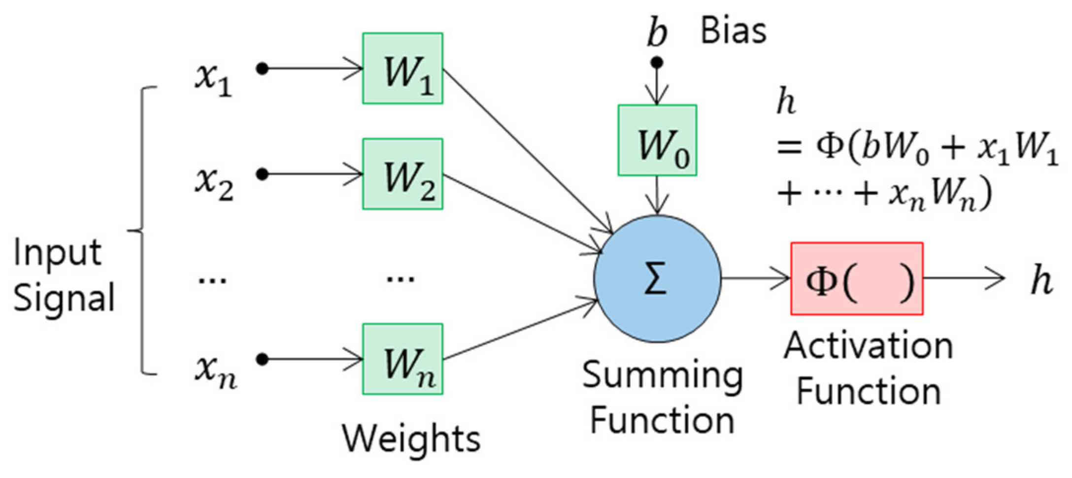
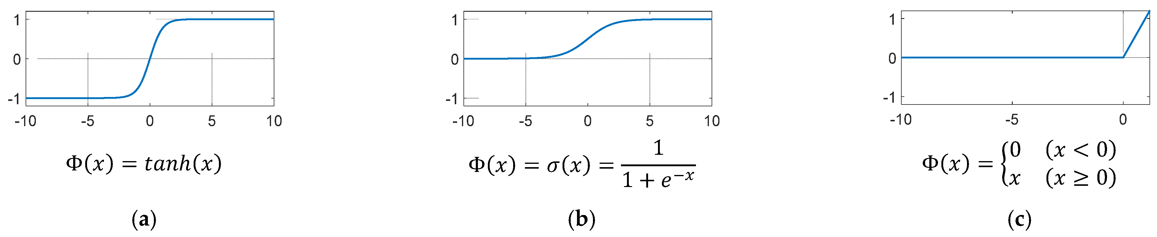
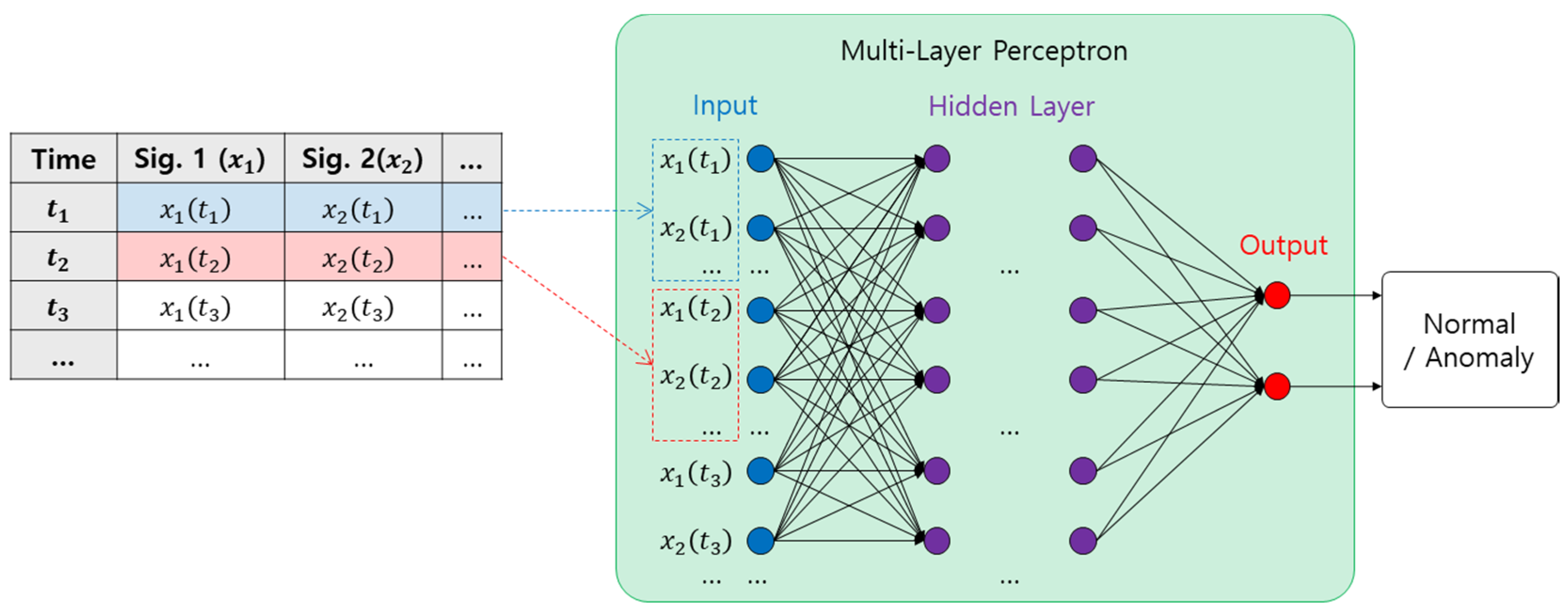
4.1. Multi-Layer Perceptron (MLP)

MLP is the neural network in the form of sequentially attaching several layers that are composed of perceptrons. Figure 4 shows the structure of the perceptron [47]. As shown in Figure 4, a single perceptron adds up all the weighted inputs and biases and then calculates an output $h$ by inputting the summed value to an activation function, shown in Figure 5.

We trained the engine clutch engagement/disengagement anomaly detection model using MLP by configuring the input/output structure as shown in Figure 6. Because MLP can receive one-dimensional input data only, the target signals for each pattern were configured and inputted in one dimension, as shown in Figure 6. Although MLP receives one-dimensional data, we expected MLP to learn data patterns because units of hidden layers are all connected to input nodes. There are also studies where MLP learned time-series data [48,49]. Before inputting data to MLP, because the length of the target signal in a pattern may be different for each pattern, it is necessary to match the length of the signal and then input it into the network. Accordingly, the data were constructed in one dimension after filling the insufficient data points with zeroes in line with the pattern that had the longest data length. Equation (1) below is the example of a pattern with a length of 5, filling the data with a length of 10. In the equation, $x_{Data}$ is the preprocessed target signal vector, and $x_{Data,Input}$ is the target signal vector that is inputted into the network; $x_{Data,Input}$ configured in this way is reorganized into one dimension in the way shown in Figure 6 and input into the network. We composed the output as normal/anomaly per pattern to determine normal/anomaly considering data trends over time. The two output units shown in Figure 6 are ${\left[\begin{array}{cc}1& 0\end{array}\right]}^T$ in the case of normal and ${\left[\begin{array}{cc}0& 1\end{array}\right]}^T$ in the case of anomaly. This output unit configuration follows the setting of the Matlab MLP training app we used. This app determines the number of output neurons as much as the number of output classes.

$$x_{Data}=\left[\begin{array}{ccc}{x}_1\left(t_1\right)& x_2\left(t_1\right)& \cdots \\ x_1\left(t_2\right)& x_2\left(t_2\right)& \cdots \\ \begin{array}{c}{x}_1\left(t_3\right)\\ x_1\left(t_4\right)\\ x_1\left(t_5\right)\end{array}& \begin{array}{c}{x}_2\left(t_3\right)\\ x_2\left(t_4\right)\\ x_2\left(t_5\right)\end{array}& \begin{array}{c}\cdots \\ \cdots \\ \cdots \end{array}\end{array}\right] ⟶ x_{Data,Input}=\left[\begin{array}{ccc}{x}_1\left(t_1\right)& x_2\left(t_1\right)& \cdots \\ x_1\left(t_2\right)& x_2\left(t_2\right)& \cdots \\ x_1\left(t_3\right)& x_2\left(t_3\right)& \cdots \\ x_1\left(t_4\right)& x_2\left(t_4\right)& \cdots \\ x_1\left(t_5\right)& x_2\left(t_5\right)& \cdots \\ 0& 0& \cdots \\ 0& 0& \cdots \\ 0& 0& \cdots \\ 0& 0& \cdots \\ 0& 0& \cdots \end{array}\right]$$

(1)

The number of hidden layers and hidden units for the MLP-based models were composed as shown in

Table 4. Hidden layer and hidden unit settings for MLP-based anomaly detection models.

Model	The Number of Hidden Layers	The Number of Hidden Units per Hidden Layer
MLP-m1	1	10
MLP-m2	2	10
MLP-m3	3	10
MLP-m4	1	100
MLP-m5	3	100

. We set these values to an appropriate value through trial and error. This configuration is for comparing training results according to the number of hidden units per hidden layer and training results according to the number of hidden layers. For a clear comparison, we composed values with large differences. A hyperbolic tangent function was used as an activation function. In the case of MLP-based models, unlike other training architectures, trained models tended to overfit when data were divided into training data and test data only. Therefore, we trained the models by dividing the data into a training, validation, and test set when training the MLP-based models. The proportions of training, validation, and test sets were 70%, 15%, and 15%, respectively, and data were randomly sampled from the data shown in Table 3.

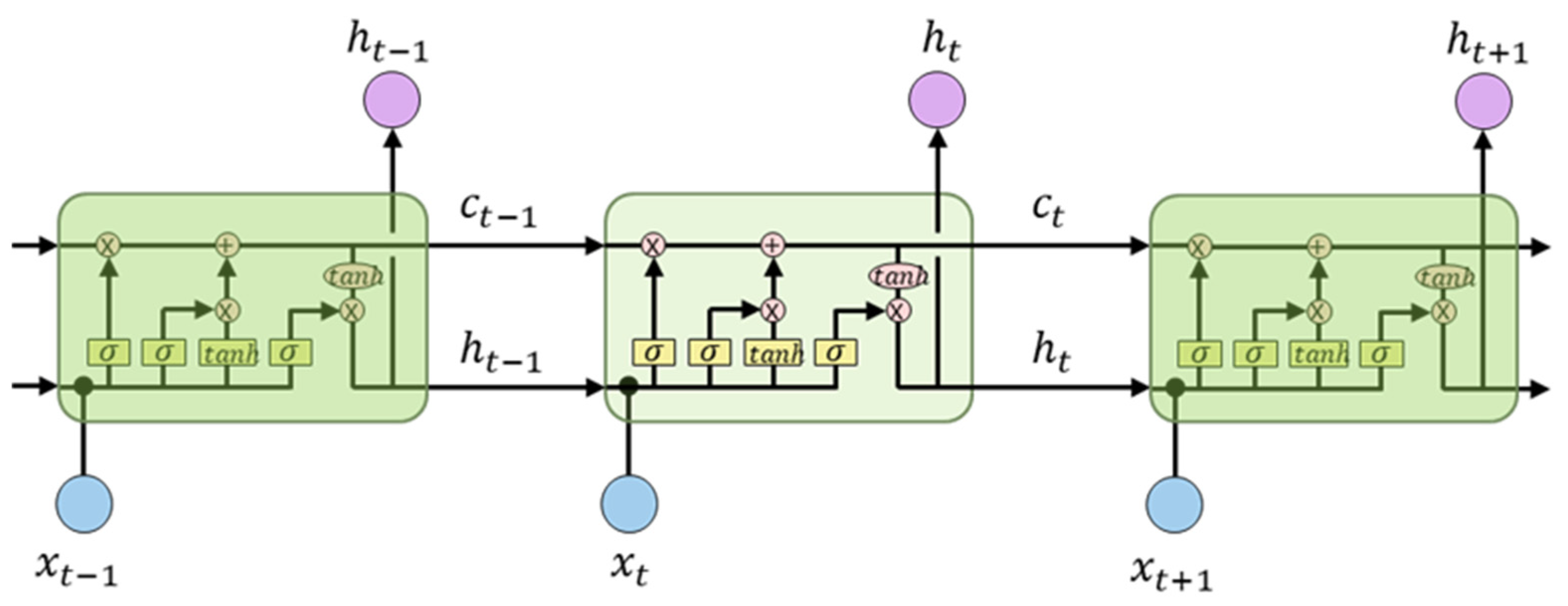
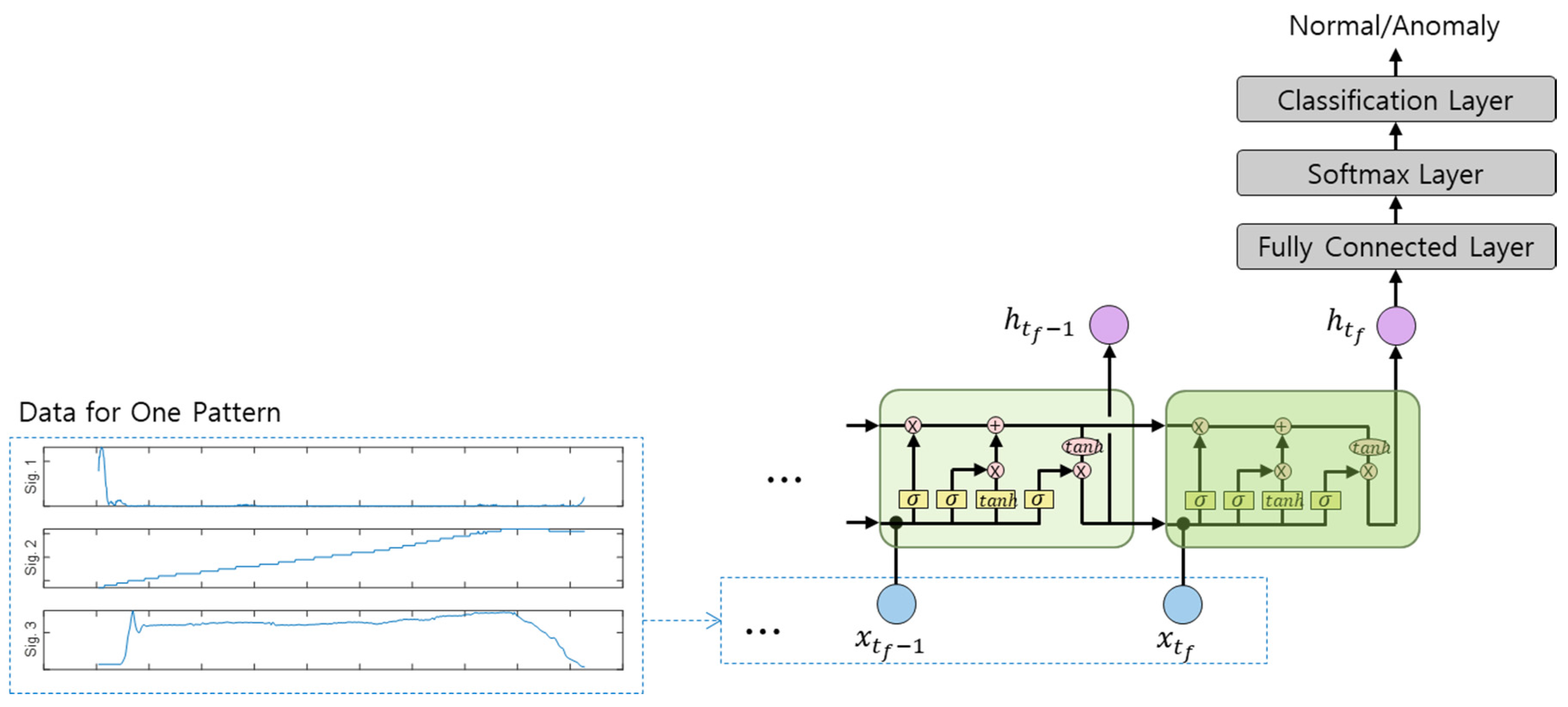
4.2. Long Short-Term Memory (LSTM)

A recurrent neural network (RNN) is mainly used to learn ordered data or time-series data such as natural language processing and speech recognition [50,51,52,53,54,55,56,57,58,59]. However, RNN has the vanishing gradient problem that significantly reduces the learning ability when the distance between the previous output and the point where it uses the information from that output is far away [60,61]. LSTM is the proposed neural network architecture to solve this vanishing gradient problem. An LSTM network is composed of connected multiple LSTM cells as shown in Figure 7 [62].

Equations (2)–(7) are the equations for an LSTM cell unit. In each equation, $W_q, U_q$, and $b_q \left(q=f, i, o, c\right)$ denote weight and bias, respectively. Here, $x_t$ represents the input vector of the LSTM cell unit, $f_t$ represents the forget gate’s activation vector, $i_t$ represents the input/update gate’s activation vector, $o_t$ represents the output gate’s activation vector, ${\tilde{c}}_t$ represents the cell input activation vector, $h_t$ represents the hidden state vector that is known as the LSTM cell unit’s output vector, and $\odot$ represents the Hadamard product [63].

$$f_t=\sigma \left(W_{f }{x}_t+U_{f }{h}_{t-1}+b_{f }\right)$$

(2)

$$i_t=\sigma \left(W_{i }{x}_t+U_{i }{h}_{t-1}+b_{i }\right)$$

(3)

$$o_t=\sigma \left(W_{o }{x}_t+U_{o }{h}_{t-1}+b_{o }\right)$$

(4)

$${\tilde{c}}_t=tanh\left(W_{c }{x}_t+U_{c }{h}_{t-1}+b_{c }\right)$$

(5)

$$c_t=f_t\odot c_{t-1}+i_t\odot {\tilde{c}}_t$$

(6)

$$h_t=o_t\odot tanh\left(c_{t }\right)$$

(7)

We trained the engine clutch engagement/disengagement anomaly detection model using LSTM by configuring the input/output structure as shown in Figure 8. The network was constructed by sequentially connecting the LSTM layer, fully connected layer, softmax layer, and classification layer, as shown in the figure. We inputted target signals per pattern into the LSTM layer and configured normal/anomaly per pattern as the output of the network. We also matched the LSTM’s input data length to the length of the longest pattern using Equation (1). The data were normalized so that the average of the input data is zero before inputting the data.

The number of LSTM layers and hidden units for the model based on LSTM were composed as shown in

Table 5. LSTM layer and hidden unit settings for the LSTM-based anomaly detection models.

Model	The Number of LSTM Layers	The Number of Hidden Units per LSTM Layer
LSTM-m1	1	200
LSTM-m2	1	400
LSTM-m3	3	100

. We set these values to an appropriate value through trial and error. This configuration is for comparing training results according to the number of hidden units per LSTM layer and training results according to the number of LSTM layers. But as there are many learning parameters for each LSTM layer, it can be overfitted if there are many layers. Therefore, to prevent this, we reduced the number of hidden units per layer if there were three LSTM layers. For training, 80% of the data shown in Table 3 were randomly sampled, and other data were used as test data.

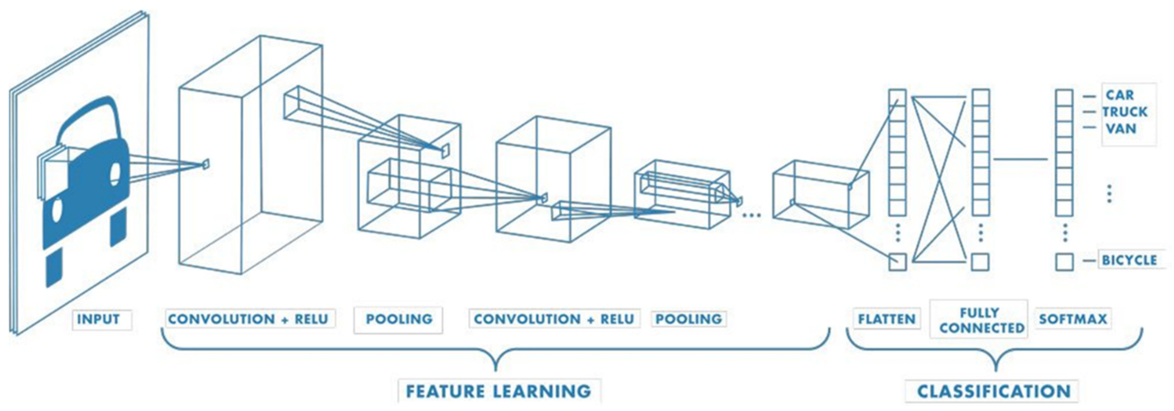
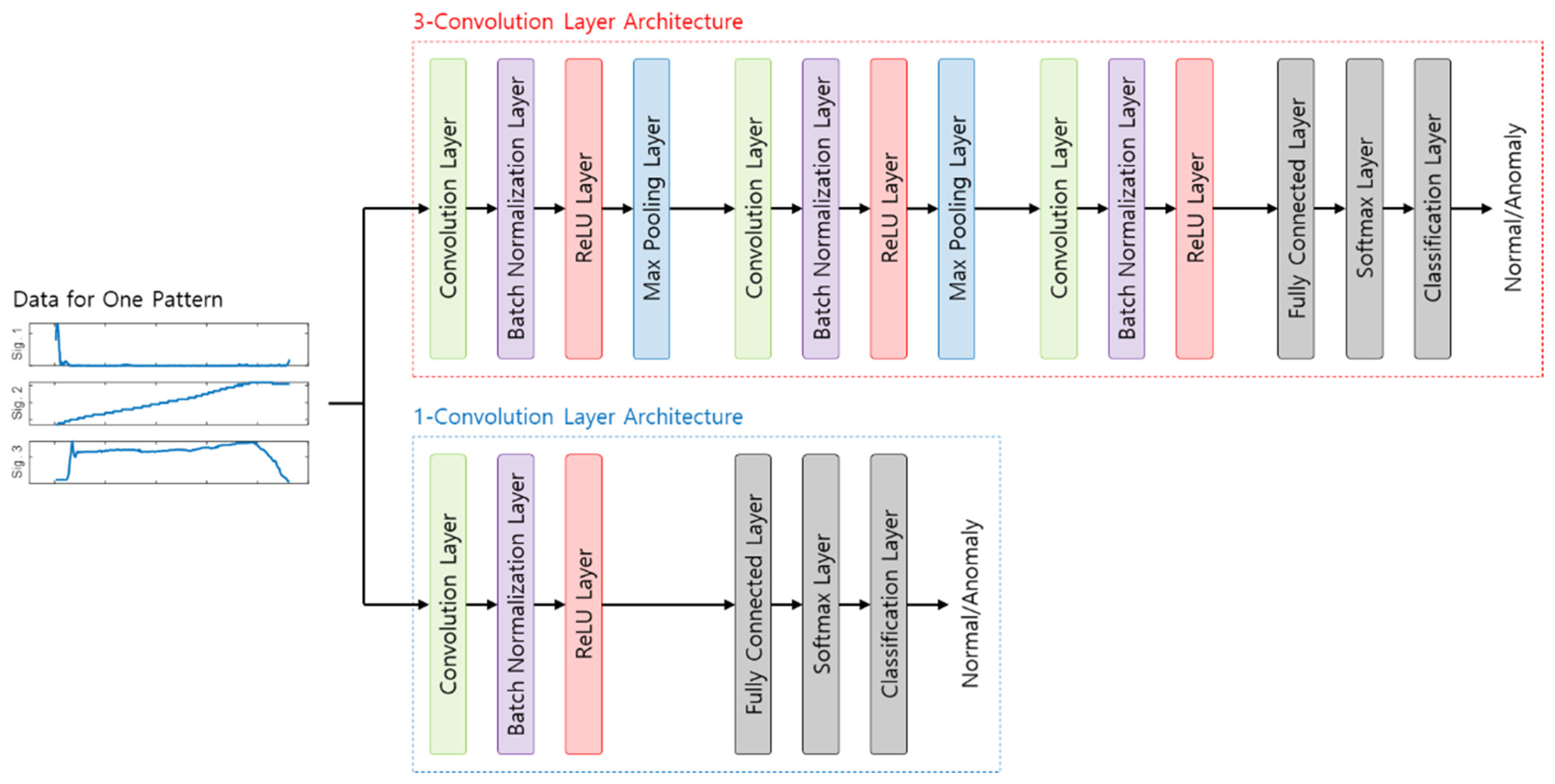
4.3. Convolutional Neural Network (CNN)

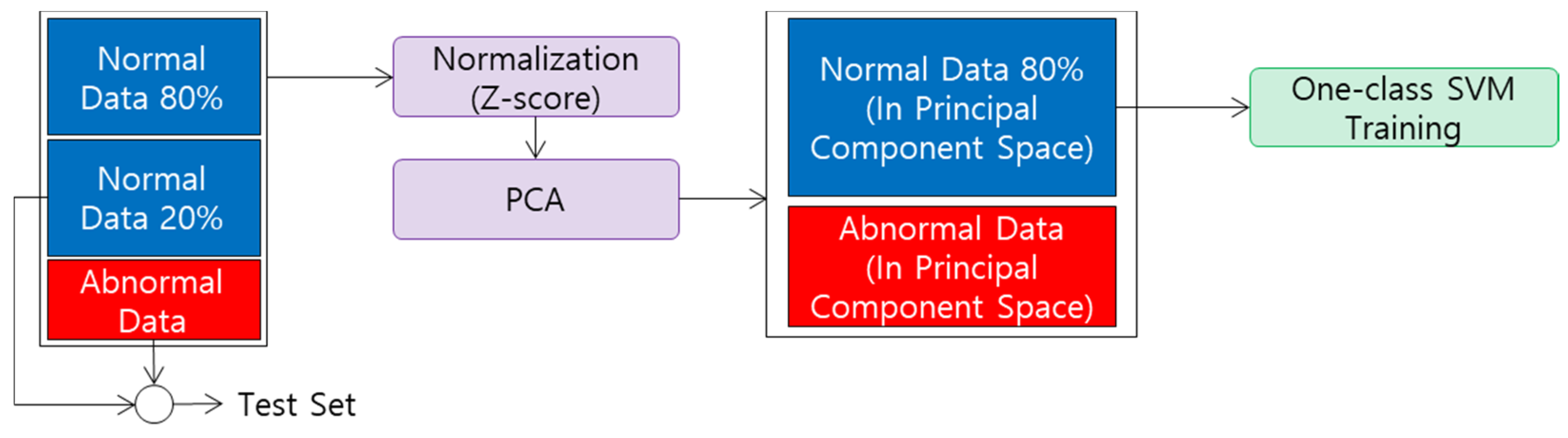
A CNN is the network architecture that learns directly from data, eliminating the need for manual feature extraction. CNNs are particularly useful for finding patterns in images to recognize objects, faces, and scenes. They can also be quite effective for classifying non-image data such as audio, time series, and signal data [64,65,66,67,68,69,70,71,72,73]. Figure 9 shows an example of image classification using a CNN [65]. As shown in the figure, a convolution operation is repeatedly performed to extract features, and extracted features are entered into the fully connected network to classify the images.

We trained the engine clutch engagement/disengagement anomaly detection model using a CNN by configuring the input/output structure as shown in Figure 10. As shown in the figure, the architectures with one and three convolution layers were constructed. In [74], the authors configured the channel for time-series data to enter the data into the convolution layer to classify time-series data. Similarly, we configured the channel for each target signal to enter the data into the first convolution layer. The output of the network is the normal/anomaly per pattern, as in the aforementioned MLP and LSTM. For input signals of the network, we matched the length of data per pattern in the same way as the MLP and LSTM, using Equation (1), and then entered the data into the network. The composition of layers for each architecture in Figure 10 is as follows. First,

Table 6. Convolutional layer hyperparameter setting.

3-Convolution Layer Architecture
Hyperparameter	1st convolutional layer	2nd convolutional layer	3rd convolutional layer
Filter size	(1, 50)	(1, 50)	(1, 50)
The number of filters	64	128	256
Stride	(1, 1)	(1, 1)	(1, 1)
1-Convolution Layer Architecture
Hyperparameter	1st convolutional layer	-	-
Filter size	(1, 50)	-	-
The number of filters	64	-	-
Stride	(1, 1)	-	-

shows the hyperparameter setting of the convolutional layer for each architecture. In the table, [w, h] of the filter size means [height, width (time axis)] of the filter, and [a, b] of the stride means [vertical step size, horizontal step size]. Because the input data is one-dimensional, the height of the filter size and vertical step size of the stride is always 1. We made the input size and output size of the layer the same by using zero padding. In the batch normalization layer, z-score normalization is conducted on input data for each channel. In the ReLU layer, the activation function shown in Figure 5c is applied to the input data. The max pooling layer performs downsampling by outputting a maximum value for a specific region (pooling region) of input data. The sizes of the pooling regions of the two max pooling layers of the 3-convolutional layer architecture were set to (1, 3) and (1, 4), respectively, and the stride values were also set to (1, 3) and (1, 4), respectively. Here, (w, h) of the pooling regions size means height, width (time axis)] of pooling region. The set values for each layer above were selected according to a general method or through trial and error.

The number of convolution layers for the model based on a CNN were composed as shown in

Table 7. Convolution layer settings for the CNN-based anomaly detection models.

Model	The Number of Convolution Layers
CNN-m1	1
CNN-m2	3

. This configuration is for comparing training results according to the number of CNN layers. For a clear comparison, we composed values with large differences. For training, 80% of the data shown in Table 3 were randomly sampled, and other data were used as test data.

4.4. One-Class SVM

Like the target data in this paper, when the number of data per class is unbalanced, a model is sometimes learned using only a class with a large number of data, which is called one-class classification [75]. One-class SVM is a representative method in one-class classification [76]. Because the target data in this study were also disproportionate in the number of normal/anomaly data, as shown in Table 2, we trained the models to detect anomalies in engine clutch engagement/disengagement data using one-class SVM and only normal data.

Figure 11 shown the engine clutch engagement/disengagement anomaly detection model training structure using one-class SVM. For effective training, we performed z-score normalization and principal component analysis (PCA). The one-class SVM model was trained with data dimensionally reduced to the principal component space through PCA. We used data projected into the three-dimensional principal component space because the principal component contribution analysis of the target signal showed that the cumulative contribution rate of the three principal components was 71–77%.

The input/output data structure for training the one-class SVM model consisted of two types. The first type consisted of target data per pattern as input and normal/anomaly per pattern as output (Type 1). The second type consisted of normal/anomaly per data instance of the target signals as output, and the input data were the same as Type 1 (Type 2). The model learned with this configuration determines the normal/anomaly state of the data instance. Training examples for each type are shown in Figure 12. However, for vehicle data, the duration of a particular situation can be a criterion for normal/anomaly status. For example, for hydraulic pressure following errors in engine clutches, the errors above a certain level for a short time may occur because it takes a certain amount of time for hydraulic pressure to be generated. This situation should be seen as normal. As configuring normal/anomaly per data instance as the output of the model makes it difficult to determine normal/anomaly for the duration of this situation, we configured the signal duration ($D{T}_k, k=1,2,\cdots$) as shown in Figure 13 as additional input data to the model. As shown in the figure, the signal duration was derived by separating the interval of the signal based on when any target signals change, and for this, continuous signals should be discretized. If the configured signal duration satisfies an anomaly criterion, all data instances in the corresponding signal interval are labeled as anomalies.

The models based on one-class SVM also learned with various hyperparameter configurations, as shown in

Table 8. Hyper parameter settings for the one-class SVM-based anomaly detection models.

Model	Model Input/Output	Discretization	Outlier Fraction [%]
One-class SVM-m1	Type 1	-	0.1
One-class SVM-m2	Type 2	Using domain knowledge	0.1
One-class SVM-m3	Type 2	Densely	0.01
One-class SVM-m4	Type 2	Densely	0.1
One-class SVM-m5	Type 2	Densely	1

. For the discretization method, the method using domain knowledge discretized the target continuous signals densely where dense discretization is required and coarsely where it is not. The area where dense discretization or coarse discretization is needed was determined by domain knowledge. Dense discretization discretized the target continuous signals to be sufficiently narrow and evenly spaced. The outlier fraction is the prediction ratio of how much anomalous data will be within the training data. A small outlier fraction means predicting that there will be fewer anomalous data within the training data and a large outlier fraction means predicting that there will be many anomalous data within the training data. In this work, we performed the one-class SVM learning with only data labeled as normal. Thus, we trained the model with small outlier fraction values. For training, 80% of the data shown in Table 3 were randomly sampled, and other data were used as test data.

5. Anomaly Detection Model Test Results

This section describes the test results of the models trained with the architectures constructed in Section 4. We used the data not used for training to test the models and compared the results using true positive rate (TPR), true negative rate (TNR), and accuracy. The TPR, TNR, and accuracy were calculated using equations (8) to (10). In the equations, TP means true positive, FN means false negative, TN means true negative, and FP means false positive.

$$TPR \left(True Positive Rate\right)=\frac{TP}{TP+FN}\times 100$$

(8)

$$TNR \left(True Negative Rate\right)=\frac{TN}{TN+FP}\times 100$$

(9)

$$Accuracy=\frac{TP+TN}{TP+TN+FP+FN}\times 100$$

(10)

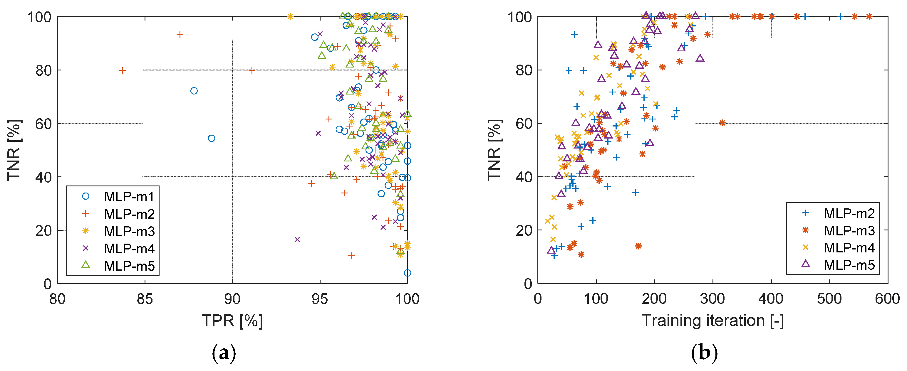
5.1. Multi-Layer Perceptron (MLP)

Unlike other architectures such as LSTM, CNN, and one-class SVM, the MLP-based anomaly detection models showed a rather large performance difference each time they were trained, even in the same hidden layers and hidden units. Therefore, we trained the MLP-based anomaly detection models for each configuration in Table 4 many times and compared the results. Figure 14a below shows the TPR and TNR results, and Figure 14b shows the TNR results according to training iteration for each model. In Figure 14a, we can see that the TPR was mostly derived high, but the TNR was often derived low. Additionally, in Figure 14b, we can see that TNR tended to appear low when the training iteration was small. That is, models with a low TNR can be viewed as local optimal. According to these results, we can conclude that the MLP-based anomaly detection models are capable of adequately distinguishing anomalies from normal, but local optimal models with a low TNR can be easily derived.

Table 9. Test results of MLP-based anomaly detection models.

Model	TPR (Average)	TNR (Average)	Accuracy (Average)
MLP-m1	97.6	70.1	90.5
MLP-m2	97.5	62.3	87.9
MLP-m3	98.4	67.2	90.5
MLP-m4	98.0	67.2	90.5
MLP-m5	97.8	72.0	91.0

shows the average values of the training results for each model. We can see that the TNRs and accuracies are lower than the TPRs because low TNR cases were often derived, as shown in Figure 14a.

5.2. Long Short-Term Memory (LSTM)

Figure 15 shows the accuracy according to the training progresses of LSTM-m2, and

Table 10. Test results of the LSTM-based anomaly detection models.

Model	TPR [%]	TNR [%]	Accuracy [%]
LSTM-m1	98.9	28.4	79.6
LSTM-m2	90.5	28.2	75.7
LSTM-m3	100	4.0	74.6

shows the training results of the models per the LSTM layers and hidden units configured as shown in Table 5. The numbers 10–90 shown above the graph’s x-axis in the figure means the number of epochs. In Figure 15, we can see that the accuracy according to the training progress is oscillating between about 60 and 90% and not converging. Training LSTM is done by dividing the training data into several subsets and finding parameters that minimize the loss function for each training data subset. The reason for accuracy oscillating is optimized LSTM parameters for each subset do not converge and continue to change. This means that the LSTM cannot properly find the pattern of target input/output data. Accordingly, we can see that the accuracy per the models in Table 10 is also low. All training results show high TPRs but low TNRs.

5.3. Convolutional Neural Network (CNN)

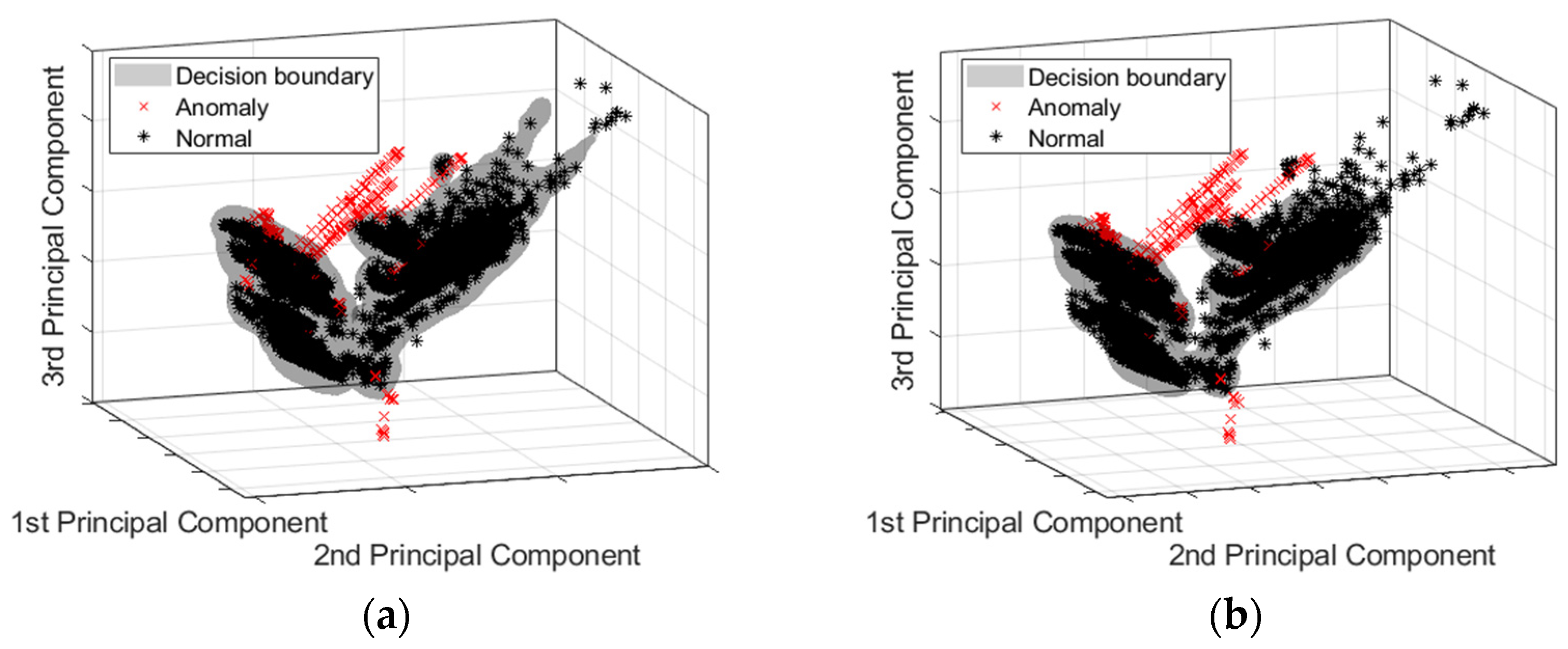
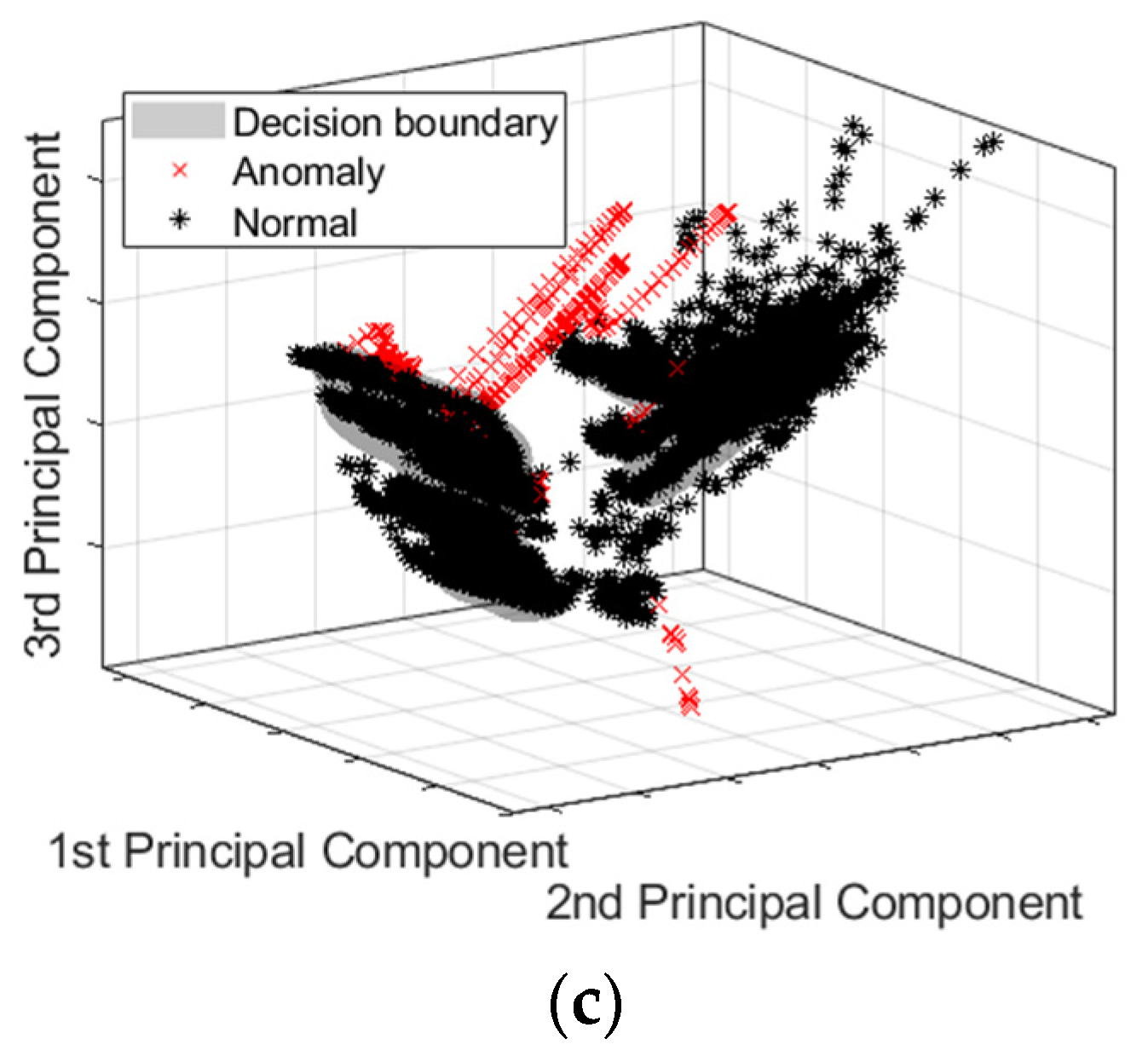
Figure 16 shows the accuracy according to the training progresses of CNN-m2, and

Table 11. Test results of the CNN-based anomaly detection models.

Model	TPR [%]	TNR [%]	Accuracy [%]
CNN-m1	100	19.8	80.6
CNN-m2	100	29.8	83.0

shows the training results of the models per the convolutional layers configured as shown in Table 7. The numbers 10–90 shown above the graph’s x-axis in the figure means the number of epochs. In Figure 16, we can see the CNN-based models are converging differently from LSTM. However, Table 11 shows that the training results of the CNN-based models have low TNRs, like LSTM-based models.

5.4. One-Class SVM

Table 12. Test results of the one-class SVM-based anomaly detection models.

Model	TPR [%]	TNR [%]	Accuracy [%]
One-class SVM-m1	56.0	83.5	66.3
One-class SVM-m2	93.3	99.9	97.9
One-class SVM-m3	96.8	100	99.0
One-class SVM-m4	97.2	99.9	99.0
One-class SVM-m5	98.2	99.0	98.7

shows the training results of the models per the hyperparameters configured as shown in Table 8. The results of one-class SVM-m2 through m5 show that both TPRs and TNRs are higher than one-class SVM-m1. Through this, we can show that, for one-class SVM, it is more appropriate to construct normal/anomaly per data instance as the output data. As for the discretization of continuous signals, the comparison between one-class SVM-m2 and one-class SVM-m3 through m5 shows that dense discretization is more advantageous for TPR. One-class SVM-m3 through m5 are the results of different outlier fractions, and we can see that the larger the outlier fraction, the higher the TPR and the lower the TNR. This is because the larger the outlier fraction, the narrower the decision boundary, as shown in Figure 17. The decision boundary is the criterion by which the model distinguishes anomalies.

The training results of each architecture and model’s configuration are summarized as follows. First, for MLP, it is possible to derive the model that adequately distinguishes normal/anomaly, but we could see the phenomenon where local optimal models with low TNRs are easily derived. The LSTM and CNN-based models also showed low TNRs. Like this, the TNRs of MLP, LSTM, and CNN all tended to have low values. This is thought to be because anomalous data have fewer numbers than normal data. Training is conducted in the direction of increasing the accuracy of the training dataset. Therefore, even if the accuracy of the class having a low number is low, if the accuracy of the class having a high number is high, the overall accuracy is increased. Since our training data also have more normal data than anomalous data, we can infer that the models were trained in this way to increase the accuracy of normal data. This can be confirmed from the high TPR results and low TNR results for each architecture. In the case of one-class SVM, the models that configured normal/anomaly per data instance as output showed high TPRs and TNRs. Through these results, we found that for engine clutch engagement/disengagement data with an imbalance in normal/anomaly, constructing the training architecture to determine normal/anomaly by data instance and performing one-class classification are advantageous for anomaly detection. In this work, we used one-class SVM, which is most commonly used for one-class classification, but other one-class classification architectures are also expected to show high anomaly detection performance.

6. Discussion

In this paper, we studied the methods for detecting anomalies in the engine clutch engagement/disengagement process required for EV↔HEV mode transitions of TMED type HEVs. We used machine learning-based methods such as MLP, LSTM, CNN, and one-class SVM and trained various models according to different parameters like the number of hidden layers and hidden units, outlier fraction, etc. For data verification at an actual vehicle level, we used the data acquired through actual vehicle tests for model training and testing. The training results showed that the models based on MLP, LSTM, and CNN have low TNRs, whereas one-class SVM-m3 though m5, the models based on one-class SVM, have high TPRs and TNRs. Through these results, we could obtain the following conclusions.

• For engine clutch engagement/disengagement data, constructing training architecture to determine normal/anomaly by data instance and performing one-class classification are advantageous for anomaly detection.
• The structure of determining normal/anomaly per pattern cannot learn characteristics of engine clutch engagement/disengagement data properly.

For the second item, the various durations of a vehicle state, such as the duration of clutch engaged, may be one of the reasons why determining normal/anomaly per the pattern is not adequate. We expected the training architectures to learn normal/anomaly for pattern regardless of the duration of the vehicle state by learning the relationship between the data at the previous time and the data at the current time. But it is presumed that the structure of determining normal/anomaly per pattern cannot learn these characteristics well.

Since most of the data acquired through real vehicle tests will have similar characteristics, one-class classification by data instance is expected to be effective for other vehicle test data. Therefore, future work should examine whether a one-class classification by data instance is also effective in detecting anomalies in other HEV powertrain control functions.

Finally, we also anticipate that real-time detection is possible because the time to detect anomalies for given data is short if there is an already trained model. But if there is no trained model, it is difficult to perform this part in real-time because training time is very long.

References

1. Kim, Y.S.; Park, J.; Park, T.W.; Bang, J.S.; Sim, H.S. Anti-jerk controller design with a cooperative control strategy in hybrid electric vehicle. In Proceedings of the 8th International Conference on Power Electronics-ECCE Asia, Jeju, Korea, 30 May–3 June 2011. [Google Scholar]
2. Anselma, P.G.; Del Prete, M.; Belingardi, G. Battery High Temperature Sensitive Optimization-Based Calibration of Energy and Thermal Management for a Parallel-through-the-Road Plug-in Hybrid Electric Vehicle. Appl. Sci. 2021, 11, 8593. [Google Scholar] [CrossRef]
3. Sim, K.; Oh, S.-M.; Kang, K.-Y.; Hwang, S.-H. A Control Strategy for Mode Transition with Gear Shifting in a Plug-In Hybrid Electric Vehicle. Energies 2017, 10, 1043. [Google Scholar] [CrossRef] [Green Version]
4. Xiao, R.; Liu, B.; Shen, J.; Guo, N.; Yan, W.; Chen, Z. Comparisons of Energy Management Methods for a Parallel Plug-In Hybrid Electric Vehicle between the Convex Optimization and Dynamic Programming. Appl. Sci. 2018, 8, 218. [Google Scholar] [CrossRef] [Green Version]
5. Maddumage, W.; Perera, M.; Attalage, R.; Kelly, P. Power Management Strategy of a Parallel Hybrid Three-Wheeler for Fuel and Emission Reduction. Energies 2021, 14, 1833. [Google Scholar] [CrossRef]
6. Zhang, Y.; Gantt, G.W.; Rychlinski, M.J.; Edwards, R.M.; Correia, J.J.; Wolf, C.E. Connected Vehicle Diagnostics and Prognostics, Concept, and Initial Practice. IEEE Trans. Reliab. 2009, 58, 286–294. [Google Scholar] [CrossRef]
7. Chen, H.; Peng, Y.; Zeng, X.; Shang, M.; Song, D.; Wang, Q. Fault Detection and Confirmation for Hybrid Electric Vehicle. In Proceedings of the 2014 IEEE Conference and Expo Transportation Electrification Asia-Pacific (ITEC Asia-Pacific), Beijing, China, 31 August–3 September 2014; pp. 1–6. [Google Scholar]
8. Song, Y.; Wang, B. Analysis and Experimental Verification of a Fault-Tolerant HEV Powertrain. IEEE Trans. Power Electron. 2013, 28, 5854–5864. [Google Scholar] [CrossRef]
9. Yang, N.; Shang, M. Common Fault Detection and Diagnosis of Santana Clutch. In Proceedings of the 2016 International Conference on Education, Management, Computer and Society, Shenyang, China, 1–3 January 2016; Atlantis Press: Shenyang, China, 2016. [Google Scholar]
10. Ferreira, D.R.; Scholz, T.; Prytz, R. Importance Weighting of Diagnostic Trouble Codes for Anomaly Detection. In Proceedings of the Machine Learning, Optimization, and Data Science, Siena-Tuscany, Italy, 19–23 July 2020; Springer International Publishing: Cham, Switzerland, 2020; pp. 410–421. [Google Scholar]
11. Pan, Y.; Feng, X.; Zhang, M.; Han, X.; Lu, L.; Ouyang, M. Internal Short Circuit Detection for Lithium-Ion Battery Pack with Parallel-Series Hybrid Connections. J. Clean. Prod. 2020, 255, 120277. [Google Scholar] [CrossRef]
12. Algredo-Badillo, I.; Ramírez-Gutiérrez, K.A.; Morales-Rosales, L.A.; Pacheco Bautista, D.; Feregrino-Uribe, C. Hybrid Pipeline Hardware Architecture Based on Error Detection and Correction for AES. Sensors 2021, 21, 5655. [Google Scholar] [CrossRef]
13. Qin, G.; Ge, A.; Li, H. On-Board Fault Diagnosis of Automated Manual Transmission Control System. IEEE Trans. Control Syst. Technol. 2004, 12, 564–568. [Google Scholar] [CrossRef]
14. Xu, L.; Li, J.; Ouyang, M.; Hua, J.; Li, X. Active Fault Tolerance Control System of Fuel Cell Hybrid City Bus. Int. J. Hydrog. Energy 2010, 35, 12510–12520. [Google Scholar] [CrossRef]
15. Tabbache, B.; Benbouzid, M.E.H.; Kheloui, A.; Bourgeot, J. Virtual-Sensor-Based Maximum-Likelihood Voting Approach for Fault-Tolerant Control of Electric Vehicle Powertrains. IEEE Trans. Veh. Technol. 2013, 62, 1075–1083. [Google Scholar] [CrossRef] [Green Version]
16. Wang, Y.; Gao, B.; Chen, H. Data-Driven Design of Parity Space-Based FDI System for AMT Vehicles. IEEE/ASME Trans. Mechatron. 2015, 20, 405–415. [Google Scholar] [CrossRef]
17. Roubache, T.; Chaouch, S.; Naït-Saïd, M.-S. Backstepping Design for Fault Detection and FTC of an Induction Motor Drives-Based EVs. Automatika 2016, 57, 736–748. [Google Scholar] [CrossRef] [Green Version]
18. Trask, S.J.H.; Jankord, G.J.; Modak, A.A.; Rahman, B.M.; Rizzoni, G.; Midlam-Mohler, S.W.; Guercioni, G.R. System Diagnosis and Fault Mitigation Strategies for an Automated Manual Transmission. In Proceedings of the ASME 2017 Dynamic Systems and Control Conference, Tysons, VA, USA, 11–13 October 2017; Volume 2, p. V002T19A001. [Google Scholar]
19. Meyer, R.T.; Johnson, S.C.; DeCarlo, R.A.; Pekarek, S.; Sudhoff, S.D. Hybrid Electric Vehicle Fault Tolerant Control. J. Dyn. Syst. Meas. Control 2018, 140, 021002. [Google Scholar] [CrossRef] [Green Version]
20. Kersten, A.; Oberdieck, K.; Bubert, A.; Neubert, M.; Grunditz, E.A.; Thiringer, T.; Doncker, R.W.D. Fault Detection and Localization for Limp Home Functionality of Three-Level NPC Inverters with Connected Neutral Point for Electric Vehicles. IEEE Trans. Transp. Electrif. 2019, 5, 416–432. [Google Scholar] [CrossRef]
21. Fill, A.; Koch, S.; Birke, K.P. Algorithm for the Detection of a Single Cell Contact Loss within Parallel-Connected Cells Based on Continuous Resistance Ratio Estimation. J. Energy Storage 2020, 27, 101049. [Google Scholar] [CrossRef]
22. Xu, J.; Wang, J.; Li, S.; Cao, B. A Method to Simultaneously Detect the Current Sensor Fault and Estimate the State of Energy for Batteries in Electric Vehicles. Sensors 2016, 16, 1328. [Google Scholar] [CrossRef] [Green Version]
23. Jeon, N.; Lee, H. Integrated Fault Diagnosis Algorithm for Motor Sensors of In-Wheel Independent Drive Electric Vehicles. Sensors 2016, 16, 2106. [Google Scholar] [CrossRef] [Green Version]
24. Na, W.; Park, C.; Lee, S.; Yu, S.; Lee, H. Sensitivity-Based Fault Detection and Isolation Algorithm for Road Vehicle Chassis Sensors. Sensors 2018, 18, 2720. [Google Scholar] [CrossRef] [PubMed] [Green Version]
25. Chen, Q.; Tian, W.; Chen, W.; Ahmed, Q.; Wu, Y. Model-Based Fault Diagnosis of an Anti-Lock Braking System via Structural Analysis. Sensors 2018, 18, 4468. [Google Scholar] [CrossRef] [Green Version]
26. Byun, Y.-S.; Kim, B.-H.; Jeong, R.-G. Sensor Fault Detection and Signal Restoration in Intelligent Vehicles. Sensors 2019, 19, 3306. [Google Scholar] [CrossRef] [Green Version]
27. Akin, B.; Ozturk, S.B.; Toliyat, H.A.; Rayner, M. DSP-Based Sensorless Electric Motor Fault-Diagnosis Tools for Electric and Hybrid Electric Vehicle Powertrain Applications. IEEE Trans. Veh. Technol. 2009, 58, 2679–2688. [Google Scholar] [CrossRef]
28. Olsson, T.; Kallstrom, E.; Gillblad, D.; Funk, P. Fault Diagnosis of Heavy Duty Machines: Automatic Transmission Clutches. In Proceedings of the International Conference on Case-Based Reasoning: Workshop on Synergies between CBR and Data Mining, Cork, Ireland, 29 September–1 October 2014. [Google Scholar]
29. Sankavaram, C.; Kodali, A.; Pattipati, K.R.; Singh, S. Incremental Classifiers for Data-Driven Fault Diagnosis Applied to Automotive Systems. IEEE Access 2015, 3, 407–419. [Google Scholar] [CrossRef]
30. Choi, S.D.; Akin, B.; Kwak, S.; Toliyat, H.A. A Compact Error Management Algorithm to Minimize False-Alarm Rate of Motor/Generator Faults in (Hybrid) Electric Vehicles. IEEE J. Emerg. Sel. Top. Power Electron. 2014, 2, 618–626. [Google Scholar] [CrossRef]
31. Källström, E.; Lindström, J.; Håkansson, L.; Karlberg, M.; Bellgran, D.; Frenne, N.; Renderstedt, R.; Lundin, J.; Larsson, J. Analysis of Automatic Transmission Vibration for Clutch Slippage Detection. In Proceedings of the the 22th International Congress on Sound and Vibration, Florence, Italy, 12–16 July 2015; p. 8. [Google Scholar]
32. Theissler, A. Detecting Known and Unknown Faults in Automotive Systems Using Ensemble-Based Anomaly Detection. Knowl. Based Syst. 2017, 123, 163–173. [Google Scholar] [CrossRef]
33. Nair, V.V.; Koustubh, B.P. Data Analysis Techniques for Fault Detection in Hybrid/Electric Vehicles. In Proceedings of the 2017 IEEE Transportation Electrification Conference (ITEC-India), Pune, India, 13–15 December 2017; pp. 1–5. [Google Scholar]
34. Moosavian, A.; Najafi, G.; Ghobadian, B.; Mirsalim, M. The Effect of Piston Scratching Fault on the Vibration Behavior of an IC Engine. Appl. Acoust. 2017, 126, 91–100. [Google Scholar] [CrossRef]
35. Becherif, M.; Péra, M.-C.; Hissel, D.; Zheng, Z. Determination of the Health State of Fuel Cell Vehicle for a Clean Transportation. J. Clean. Prod. 2018, 171, 1510–1519. [Google Scholar] [CrossRef] [Green Version]
36. Kordes, A.; Wurm, S.; Hozhabrpour, H.; Wismüller, R. Automatic Fault Detection Using Cause and Effect Rules for In-Vehicle Networks. In Proceedings of the 4th International Conference on Vehicle Technology and Intelligent Transport Systems, Funchal, Portugal, 16–18 March 2018; pp. 537–544. [Google Scholar]
37. Yu, H.; Langari, R. A Neural Network-Based Detection and Mitigation System for Unintended Acceleration. J. Frankl. Inst. 2018, 355, 4315–4335. [Google Scholar] [CrossRef]
38. Ostapenko, D.I.; Fisch, J. Predictive Maintenance Using MATLAB: Pattern Matching for Time Series Data. Available online: https://www.matlabexpo.com/content/dam/mathworks/mathworks-dot-com/images/events/matlabexpo/de/2018/predictive-maintenance-with-matlab--time-series-production-data-analysis.pdf (accessed on 29 October 2021).
39. Ginzarly, R.; Hoblos, G.; Moubayed, N. From Modeling to Failure Prognosis of Permanent Magnet Synchronous Machine. Appl. Sci. 2020, 10, 691. [Google Scholar] [CrossRef] [Green Version]
40. Xu, Y.; Huang, B.; Yun, Y.; Cattley, R.; Gu, F.; Ball, A.D. Model Based IAS Analysis for Fault Detection and Diagnosis of IC Engine Powertrains. Energies 2020, 13, 565. [Google Scholar] [CrossRef] [Green Version]
41. Ewert, P.; Orlowska-Kowalska, T.; Jankowska, K. Effectiveness Analysis of PMSM Motor Rolling Bearing Fault Detectors Based on Vibration Analysis and Shallow Neural Networks. Energies 2021, 14, 712. [Google Scholar] [CrossRef]
42. Jiang, J.; Cong, X.; Li, S.; Zhang, C.; Zhang, W.; Jiang, Y. A Hybrid Signal-Based Fault Diagnosis Method for Lithium-Ion Batteries in Electric Vehicles. IEEE Access 2021, 9, 19175–19186. [Google Scholar] [CrossRef]
43. Ding, N.; Ma, H.; Zhao, C.; Ma, Y.; Ge, H. Data Anomaly Detection for Internet of Vehicles Based on Traffic Cellular Automata and Driving Style. Sensors 2019, 19, 4926. [Google Scholar] [CrossRef] [PubMed] [Green Version]
44. Moavenian, M. Fault Detection and Isolation of Vehicle Driveline System. Int. J. Automot. Eng. 2012, 2, 11. [Google Scholar]
45. Xue, Q.; Zhang, X.; Teng, T.; Zhang, J.; Feng, Z.; Lv, Q. A Comprehensive Review on Classification, Energy Management Strategy, and Control Algorithm for Hybrid Electric Vehicles. Energies 2020, 13, 5355. [Google Scholar] [CrossRef]
46. Kim, H.; Kim, J.; Lee, H. Mode Transition Control Using Disturbance Compensation for a Parallel Hybrid Electric Vehicle. Proc. Inst. Mech. Eng. Part D J. Automob. Eng. 2011, 225, 150–166. [Google Scholar] [CrossRef]
47. Gardner, M.W.; Dorling, S.R. Artificial Neural Networks (the Multilayer Perceptron)—a Review of Applications in the Atmospheric Sciences. Atmos. Environ. 1998, 32, 2627–2636. [Google Scholar] [CrossRef]
48. Widiasari, I.R.; Nugroho, L.E. Deep Learning Multilayer Perceptron (MLP) for Flood Prediction Model Using Wireless Sensor Network Based Hydrology Time Series Data Mining. In Proceedings of the 2017 International Conference on Innovative and Creative Information Technology (ICITech), Salatiga, Indonesia, 2–4 November 2017; pp. 1–5. [Google Scholar]
49. Kanchymalay, K.; Salim, N.; Sukprasert, A.; Krishnan, R.; Hashim, U.R. Multivariate Time Series Forecasting of Crude Palm Oil Price Using Machine Learning Techniques. IOP Conf. Ser. Mater. Sci. Eng. 2017, 226, 012117. [Google Scholar] [CrossRef]
50. Gulli, A.; Kapoor, A.; Pal, S. Deep Learning with TensorFlow 2 and Keras Regression, ConvNets, GANs, RNNs, NLP, and More with TensorFlow 2 and the Keras API, 2nd ed.; Packt Publishing Ltd.: Birmingham, UK, 2019; ISBN 978-1-83882-341-2. [Google Scholar]
51. Ma, Y.; Chang, Q.; Lu, H.; Liu, J. Reconstruct Recurrent Neural Networks via Flexible Sub-Models for Time Series Classification. Appl. Sci. 2018, 8, 630. [Google Scholar] [CrossRef] [Green Version]
52. Li, Q.; Xu, Y. VS-GRU: A Variable Sensitive Gated Recurrent Neural Network for Multivariate Time Series with Massive Missing Values. Appl. Sci. 2019, 9, 3041. [Google Scholar] [CrossRef] [Green Version]
53. Zhang, X.; Zhao, M.; Dong, R. Time-Series Prediction of Environmental Noise for Urban IoT Based on Long Short-Term Memory Recurrent Neural Network. Appl. Sci. 2020, 10, 1144. [Google Scholar] [CrossRef] [Green Version]
54. Elsaraiti, M.; Merabet, A. Application of Long-Short-Term-Memory Recurrent Neural Networks to Forecast Wind Speed. Appl. Sci. 2021, 11, 2387. [Google Scholar] [CrossRef]
55. Ye, F.; Yang, J. A Deep Neural Network Model for Speaker Identification. Appl. Sci. 2021, 11, 3603. [Google Scholar] [CrossRef]
56. Zhang, X.; Kuehnelt, H.; De Roeck, W. Traffic Noise Prediction Applying Multivariate Bi-Directional Recurrent Neural Network. Appl. Sci. 2021, 11, 2714. [Google Scholar] [CrossRef]
57. Ramos, R.G.; Domingo, J.D.; Zalama, E.; Gómez-García-Bermejo, J. Daily Human Activity Recognition Using Non-Intrusive Sensors. Sensors 2021, 21, 5270. [Google Scholar] [CrossRef]
58. Ankita; Rani, S.; Babbar, H.; Coleman, S.; Singh, A.; Aljahdali, H.M. An Efficient and Lightweight Deep Learning Model for Human Activity Recognition Using Smartphones. Sensors 2021, 21, 3845. [Google Scholar] [CrossRef]
59. Zhou, K.; Liu, Y. Early-Stage Gas Identification Using Convolutional Long Short-Term Neural Network with Sensor Array Time Series Data. Sensors 2021, 21, 4826. [Google Scholar] [CrossRef]
60. Hochreiter, S. The Vanishing Gradient Problem During Learning Recurrent Neural Nets and Problem Solutions. Int. J. Unc. Fuzz. Knowl. Based Syst. 1998, 06, 107–116. [Google Scholar] [CrossRef] [Green Version]
61. Bengio, Y.; Simard, P.; Frasconi, P. Learning Long-Term Dependencies with Gradient Descent Is Difficult. IEEE Trans. Neural Netw. 1994, 5, 157–166. [Google Scholar] [CrossRef] [PubMed]
62. Understanding LSTM Networks—Colah’s Blog. Available online: http://colah.github.io/posts/2015-08-Understanding-LSTMs/ (accessed on 11 June 2021).
63. Long Short-Term Memory. Wikipedia 2021. Available online: https://en.wikipedia.org/wiki/Long_short-term_memory (accessed on 29 October 2021).
64. Bengio, Y.; Goodfellow, I.; Courville, A. Deep Learning; MIT Press: Cambridge, MA, USA, 2016. [Google Scholar]
65. Convolutional Neural Network. Available online: https://ww2.mathworks.cn/en/discovery/convolutional-neural-network-matlab.html (accessed on 7 May 2021).
66. Lee, S.; Lee, Y.-S.; Son, Y. Forecasting Daily Temperatures with Different Time Interval Data Using Deep Neural Networks. Appl. Sci. 2020, 10, 1609. [Google Scholar] [CrossRef] [Green Version]
67. Zhou, Z.; Zi, Y.; Xie, J.; Chen, J.; An, T. The Next Failure Time Prediction of Escalators via Deep Neural Network with Dynamic Time Warping Preprocessing. Appl. Sci. 2020, 10, 5622. [Google Scholar] [CrossRef]
68. Nam, J.; Kang, J. Classification of Chaotic Signals of the Recurrence Matrix Using a Convolutional Neural Network and Verification through the Lyapunov Exponent. Appl. Sci. 2021, 11, 77. [Google Scholar] [CrossRef]
69. Wang, C.; Sun, H.; Zhao, R.; Cao, X. Research on Bearing Fault Diagnosis Method Based on an Adaptive Anti-Noise Network under Long Time Series. Sensors 2020, 20, 7031. [Google Scholar] [CrossRef]
70. Li, J.; Hu, D.; Chen, W.; Li, Y.; Zhang, M.; Peng, L. CNN-Based Volume Flow Rate Prediction of Oil–Gas–Water Three-Phase Intermittent Flow from Multiple Sensors. Sensors 2021, 21, 1245. [Google Scholar] [CrossRef] [PubMed]
71. Shi, X.; Huang, G.; Hao, X.; Yang, Y.; Li, Z. A Synchronous Prediction Model Based on Multi-Channel CNN with Moving Window for Coal and Electricity Consumption in Cement Calcination Process. Sensors 2021, 21, 4284. [Google Scholar] [CrossRef]
72. Al-Qershi, F.; Al-Qurishi, M.; Aksoy, M.S.; Faisal, M.; Algabri, M. A Time-Series-Based New Behavior Trace Model for Crowd Workers That Ensures Quality Annotation. Sensors 2021, 21, 5007. [Google Scholar] [CrossRef] [PubMed]
73. Theodoropoulos, P.; Spandonidis, C.C.; Giannopoulos, F.; Fassois, S. A Deep Learning-Based Fault Detection Model for Optimization of Shipping Operations and Enhancement of Maritime Safety. Sensors 2021, 21, 5658. [Google Scholar] [CrossRef] [PubMed]
74. Zhao, B.; Lu, H.; Chen, S.; Liu, J.; Wu, D. Convolutional Neural Networks for Time Series Classification. J. Syst. Eng. Electron. 2017, 28, 162–169. [Google Scholar] [CrossRef]
75. Khan, S.S.; Madden, M.G. One-Class Classification: Taxonomy of Study and Review of Techniques. Knowl. Eng. Rev. 2014, 29, 345–374. [Google Scholar] [CrossRef] [Green Version]
76. Khan, S.S.; Madden, M.G. A Survey of Recent Trends in One Class Classification. In Proceedings of the Artificial Intelligence and Cognitive Science, Dublin, Ireland, 19–21 August 2009; Coyle, L., Freyne, J., Eds.; Springer: Berlin/Heidelberg, Germany, 2009; pp. 188–197. [Google Scholar]
Figure 1. Powertrain structure of the target vehicle.
Applsci 11 10187 g001
Figure 2. Parallel HEV structures classification.
Applsci 11 10187 g002
Figure 3. An example of target data section extraction (pattern extraction).
Applsci 11 10187 g003
Figure 4. Structure of a perceptron.
Applsci 11 10187 g004
Figure 5. Activation functions for MLP: (a) hyperbolic tangent function; (b) sigmoid Function; (c) ReLU function.
Applsci 11 10187 g005
Figure 6. MLP-based anomaly detection model training architecture.
Applsci 11 10187 g006
Figure 7. LSTM architecture.
Applsci 11 10187 g007
Figure 8. LSTM-based anomaly detection model training architecture.
Applsci 11 10187 g008
Figure 9. Image classification example using a CNN.
Applsci 11 10187 g009
Figure 10. CNN-based anomaly detection model training architecture.
Applsci 11 10187 g010
Figure 11. One-class SVM-based anomaly detection model training architecture.
Applsci 11 10187 g011
Figure 12. An example of one training example for each input/output data structure type.
Applsci 11 10187 g012
Figure 13. Derivation process of signal duration.
Applsci 11 10187 g013
Figure 14. Training results of the MLP-based anomaly detection models: (a) TPR and TNR for each model training; (b) TNR according to training iteration.
Applsci 11 10187 g014
Figure 15. Accuracy according to the training progress (LSTM-m2).
Applsci 11 10187 g015
Figure 16. Accuracy according to the training progress (CNN-m2).
Applsci 11 10187 g016
Figure 17. Decision boundaries of the one-class SVM-based anomaly detection models based on the outlier fraction: (a) outlier fraction = 0.01 [%]; (b) outlier fraction = 0.1 [%]; (c) outlier fraction = 1 [%].
Applsci 11 10187 g017aApplsci 11 10187 g017b