
Design and Stiffness Optimization of Bionic Docking Mechanism for Space Target Acquisition


School of Automation, Beijing University of Posts and Telecommunications, Beijing 100876, China
*
Author to whom correspondence should be addressed.
Appl. Sci. 2021, 11(21), 10278; https://0-doi-org.brum.beds.ac.uk/10.3390/app112110278
Submission received: 11 October 2021
/
Revised: 28 October 2021
/
Accepted: 29 October 2021
/
Published: 2 November 2021
(This article belongs to the Topic Bioreactors: Control, Optimization and Applications)
Abstract
:Featured Application
In the process of space target acquisition, problems include not only the acquisition problem, but also how to buffer the collision energy, avoid collisions and reduce the impact of docking. A bionic docking mechanism with stiffness optimization for space target acquisition is designed and simulated to realize the buffering and unloading of a six–dimensional spatial collision caused by space target docking. The research results are useful with regard to the stabilization control of the spaceborne capture mechanism with future bionic docking mechanisms.
Abstract
Aiming at the soft contact problem of space docking, a bionic docking mechanism for space target acquisition is proposed to realize the buffering and unloading of six–dimensional spatial collision through flexible rotating and linear components. Using the Kane method, an integrated dynamic equation of the bionic docking mechanism in space docking is established, and the stiffness optimization strategy is carried out based on angular momentum conservation. Based on the particle swarm optimization (PSO), a stiffness optimization scheme was realized. Through the numerical simulation of the bionic docking mechanism in space docking, the stiffness optimization was achieved and the soft contact machine process is verified. Finally, through the docking collision experiments in Adams, the results indicate that the proposed bionic docking mechanism can not only prolong the collision time to win time for space acquisition, but also buffer and unload the six–dimensional spatial collision caused by space target docking.
1. Introduction
As the key equipment for space target acquisition, space docking and transposition is the core technology that all aerospace powers strive to develop [1,2,3,4,5]. At present, space docking transposition is required not only to solve the acquisition of spacecraft, but also to buffer collision energy, avoid serious collisions and reduce the impact of docking. The realization of soft docking in space on orbit acquisition is of great significance to complete the space on orbit acquisition task.
In recent years, the design of new space docking mechanisms to realize soft docking is still a research hotspot of many scholars Feng et al. [6] developed a new type of end effector prototype by combining the tendon–sheath transmission system with a steel cable snaring mechanism. Liu Yang et al. [7] designed and studied a variable topology 3–RSR polyhedron docking mechanism, and verified the practicability of the structure; Li et al. [8] designed a light and small three arm noncooperative target satellite docking mechanism. Zhang [9], et al. developed a flux pinned docking mechanism (FPDM), and designed and established the experimental demonstration system. Sohal et al. [10] proposed an integrated active genderless docking mechanism which allows for efficient docking while tolerating misalignments. Shi et al. [11] established a novel model of space electromagnetic docking to solve the problem of traditional plume contamination and short service life. Zhang et al. [12] presented one novel docking mechanism with a T–type locking structure and proved the rationality of the proposed mechanism. Chen et al. [13] studied the movement space of the LIDM’s capture system and proposed the main factors affecting the movement space. Han et al. [14] studied the innovational design technique of a docking cone and developed a new satisfactory docking cone. Moubarak et al. [15] studied the application of two–bar slider rocker mechanisms in three–state rigid active docking, and verified its effectiveness through experiments. Zhang et al. [16] proposed ahigh temperature superconducting magnetic docking mechanism which consisted of a high temperature superconductor (HTS) bulk installed on a target spacecraft module and an electromagnet installed on a tracking spacecraft module based on the flux pinning effect of an HTS.
Meanwhile, by discussing the influence of docking mechanism parameters on the soft docking of the micro satellite, many scholars proposed new docking strategies based on the existing docking mechanisms, and verified their effectiveness through simulation experiments. Bin et al. [17] verified the feasibility of realizing the action of the butt ring with the multi–motor combined control based on the scaled docking mechanism prototype of an aluminum alloy. Xu et al. [18] proposed a prediction model for the transmission error of CDS based on their cable deformation to improve the assembly efficiency of docking locks. Zhang et al. [19] established the model of grasping docking mechanism by using the mathematical methods, and analyzed the contact and collision problems in the process of grasping. Olivieri et al. [20] proposed a new docking mechanism that provides the basis for the connection and separation of small spacecraft in space. Li et al. [21] proposed a feasible docking mechanism based on the non–cooperative target docking technology points, and verified its effectiveness. Taking successful docking as the evaluation standard, Zhang et al. [22] discussed the influence of docking mechanism parameters on micro/small satellite soft docking. Zhang et al. [23] investigated the problems of spacecraft self– and soft–docking via coupled actuation of magnetic fields.
The aforementioned research on the space docking mechanism mainly focuses on the development of the capture mechanism end–effect device, as well as the contact mode and contact strategy research, but the manipulator was not employed as part of the docking mechanism. In this regard, some scholars have studied the momentum, angular momentum, and the trajectory planning of the space–borne capture mechanism.
Beginning from the flexible control and motion planning of the spaceborne capture mechanism, Wei et al. [24] proposed the impedance control method of flexible manipulator assisted large load space cabin docking and verified its effectiveness. Cong and Sun [25] proposed “straight arm grabbing”, which is the most ideal state, but it is difficult for planar robots to achieve. Based on dual–arm sport robot, Guo et al. [26] calculated the pre–impact configuration to minimize the effects of impacts on the robot ‘s angular momentum by use of the particle swarm optimizer. Hu et al. [27] presented a method to minimize the impact force by pre–impact configuration designing. Gan et al. [28] proposed a method of stiffness design for a spatial three degrees of freedom serial compliant manipulator with the objective of protecting the compliant joint actuators when the manipulator comes up against impact. Hu et al. [29] presented a method to minimize the base attitude disturbance of a space robot during target capture. Song et al. [30] proposed performance indices for impact force reduction capability and maximum speed of variable stiffness robots based on the impact ellipsoid. Oki [31] stabilized the tumbling target satellite by using time optimal control of a free–floating robot. Chen et al. [32] put forward a motion planning method for space robotic systems keeping the base inertially fixed while performing on–orbit services, using a combination of point–to–point planning and a balance–arm. Xu et al. [33] proposed a dual–arm coordinated ‘Area–Oriented Capture’ (AOC) method to capture a non–cooperative tumbling target, which has larger pose tolerance and takes shorter time for capturing a tumbling target. Larouche [34] adopted a motion prediction control scheme for autonomous acquisition tasks. Zhang [35] studied a manipulator trajectory plan by adjusting the pose of the robotic–arm and minimizing attitude disturbance of the base. However, due to the inevitable existence of model errors and operational precision, it is impossible to fundamentally avoid the impact and disturbance of the capture process, and it is difficult to suppress the complex vibration after docking.
In addition, the realization of soft docking of spatial docking through novel vibration suppression approaches has attracted more and more attention. Chu [36] applied controllable damping to the interior of the manipulator and minimized the impact of space docking on the free–floating base through a particle swarm optimization (PSO) algorithm. Nguyen [37] applied the controllable MR damper [38] to a planar 2–DOF manipulator for spatial capture, but the spatial collision problem is not resolved. In addition, Yu et al. [39] investigated spatial dynamics and control of a 6–DOF space robot with flexible panels, and indicated that flexible panels have big influence on impact dynamic characteristics. Bian [40] applied an effective shock absorber to unload the non–linear vibration of the manipulator based on the principle of internal resonance. However, to our knowledge, there is little research that mentions designing a bionic structure for soft contact to realize the buffering and unloading of six–dimensional spatial collision.
Motivated by the above observations, this paper attempts to design a bionic docking mechanism for space target acquisition, and proposes an integrated dynamic equation of spaceborne capture mechanism coupled with the proposed bionic docking mechanism. The main contributions are listed as follows.
(1) A bionic docking mechanism for space target acquisition is designed to realize the buffering and unloading of spatially six–dimensional collision caused by space target docking.
(2) An integrated dynamic equation of the bionic docking mechanism in space docking and a stiffness optimization strategy based on the angular momentum conservation are proposed.
(3) Facing the optimization of the bionic docking mechanism, the stiffness coefficients of torsion springs and linear spring are considered as particle swarms and the particle swarm optimization (PSO) algorithm is adopted to realize stiffness optimization. Numerical simulation and prototype experiments are carried out to verify the effectiveness.
The rest of this paper is organized as follows. In Section 2, we introduce the structure and function of the proposed bionic docking mechanism. Section 3 gives the dynamic equations based on Kane approach. In Section 4, a control scheme employing particle swarm optimization (PSO) is proposed. Section 5 and Section 6 can separately provide simulation examples and experiment results to verify the proposed approach and principle. Finally, we conclude all of the work in Section 7.
2. Structure of Bionic Docking Mechanism
The bionic docking mechanism includes gyro–structure assembly and sliding structure assembly to buffer and unload the six–dimensional spatial collision. A 3D model of the bionic docking mechanism is shown in Figure 1 and the generalized model of capturing mechanism with the bionic docking mechanism is shown in Figure 2. The gyro–structure assembly includes a gyro mechanism, a flexible rotating component and encoder, and the sliding–structure assembly includes a sliding mechanism, a flexible linear component and a linear displacement sensor.
In the spatial Cartesian coordinate system, the pitch and yaw directions of the gyro mechanism are taken as the X and Y axes. The 3D model of the gyro–structure assembly is shown in Figure 3 and the 3D model of the sliding–structure assembly is shown in Figure 4. In order to describe the proposed bionic docking mechanism, in this paper, Gyro–X is the X–rotation axis of the gyro mechanism, Gyro–Y is the Y–rotation axis of the gyro mechanism, Gyro–Z is the Z–rotation axis of the gyro mechanism, and Slide–Z is the Z–line axis of the sliding mechanism. The gyro mechanism can be divided into three rotating joints, in which the rotation mechanism composed of gyro frame 2 (8) rotating around Gyro–X relative to gyro frame 1 (7) is called Gyro–X joint, the rotation mechanism composed of gyro frame 3 (3) rotating around Gyro–Y relative to gyro frame 2 (8) is called Gyro–Y joint, and the rotation mechanism composed of sliding frame 1 (4) rotating around Gyro–Z relative to gyro frame 3 (3) is called Gyro–Y joint. And the sliding mechanism composed of sliding frame 2 (13) moving along Slide Z relative to sliding frame 1 is Slide Z joint. The bionic docking mechanism mainly imitates wrist movement through the spatial 3D rotation of the gyro mechanism. As shown in Figure 1 and Figure 3a, taking the palm plane as the Cartesian plane, the Gyro–X joint can imitate the upward turning motion of the wrist, it can imitate the lateral turning motion of the wrist, and it can imitate the rotation motion of the wrist around the arm.
The gyro mechanism and sliding mechanism can transfer the six–dimensional collision caused by spatially docking, and the flexible rotating component and flexible linear component can avoid the instability of the free–floating base and stabilize the bionic docking mechanism by damping vibration absorption. The flexible rotating component is composed of a rotating MR damper (2), electromagnetic clutch (5), and torsion spring (6), as shown in Figure 3a. The flexible linear component is composed of a linear spring (9), an electromagnetic braking slide (10), a linear MR damper (11) and a slider (12), as shown in Figure 3b. The rotating MR damper, torsion spring, linear MR damper and linear spring can realize the unloading and buffering of a six–dimensional spatial collision, and the electromagnetic clutch and the electromagnetic braking slide can realize the braking of the bionic docking mechanism after space target acquisition. The encoders and linear displacement sensor can measure the motion parameters of the gyro mechanism and the sliding mechanism for the closed–loop control of the spatially soft docking.
The bionic docking mechanism has four DOFs: a Gyro–X joint, a Gyro–Y joint, a Gyro–Z joint, and a Slide–Z joint to realize the buffering and unloading of a space six–dimensional collision. After the spatially 3D angular, X–line and Y–line collision are transmitted by the gyro mechanism and buffered by the torsion springs, and the damping outputs of the rotating MR damper in the Gyro–X joint, the Gyro–Y joint and the Gyro–Z joint can be planned to realize the stabilization of the gyro–structure assembly. After the spatially Z–line collision is transmitted by the sliding mechanism and buffered by the linear spring, the stabilization of the sliding–structure assembly can be realized by planning the damping output of the linear MR damper in the Slide–Z joint so as to realize the buffering and unloading of the collision of a six–dimensional spatial collision.
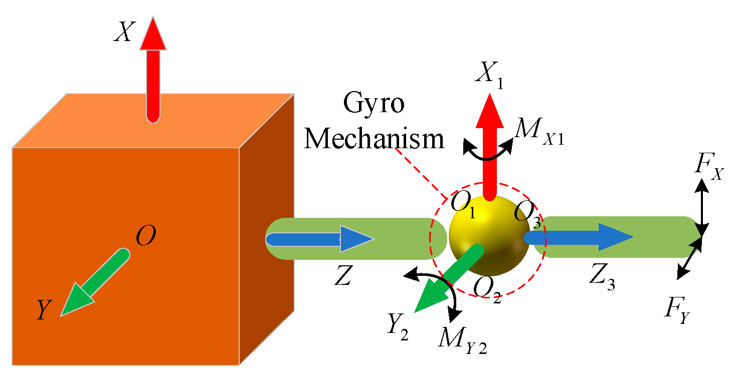
The transmission schematic of the spatially X–line and Y–line collision is shown in Figure 4, in which , and are Gyro–X, Gyro–Y and Gyro–Z respectively. The collision force () of the X direction can be converted into a torque () around the Gyro–Y. Similarly, the collision force () in the Y direction can be converted into a torque () around the Gyro–X. It can be seen that the flexible rotating components in the Gyro–X, and Gyro–Y can indirectly stabilize the collision along the Y–line and X–line collision force, so as to realize the buffering and unloading of the six–dimensional spatial collision.
3. Model of Bionic Docking Mechanism
In order to verify the effectiveness of the proposed bionic docking mechanism, a dynamic model of the bionic docking mechanism in space docking is established, as shown in Figure 5. is the inertial coordinate system, (k = 1, 2, 3, 4, 5) is the connected coordinate system of the free–floating base with the gyro frame 1, gyro frame 2, gyro frame 3 gyro frame 3, sliding frame 1 and sliding frame 2.
The flexible rotating components and the flexible linear component are arranged on the Gyro–X, Gyro–Y, Gyro–Z, and Slide–Z. It can be seen from Section 2 that the bionic docking mechanism can buffer and unload the six–dimensional spatial collision. In this section, the Kane method is used to build the integrated dynamic model of the bionic docking mechanism in space docking, and the dynamic analysis of optimization strategy of the bionic docking mechanism is proposed based on the angular momentum conservation.
3.1. Kinematics Equation
Establish the absolute inertial coordinate system , and establish the conjoined coordinate system at the end face of segment k (k = 1, 2, 3, 4, 5). The linear velocity and angular velocity of the relative motion between two adjacent segments and are selected as the generalized velocity , and meanwhile the linear displacement and angular displacement are selected as the generalized coordinates (l = 1, 2, 3,…, 10), that is:
where
is used to store generalized coordinates;
is used to store generalized velocity.
Then the relative rotation matrix of the connected coordinate system in segment k and (k − 1) is:
where
is the 3 × 3 identity matrix.
Then the absolute rotation matrix of the segment connected coordinate system relative to the inertial system OXYZ is:
Since the base has three rotational DOFs, it is assumed that coordinate system connected to the base first rotates around the axis of the inertial coordinate system and the angular velocity is , then around the axis of the coordinate system connected to the base, the angular velocity is , and finally around the axis of the coordinate system connected to the rotated base, the angular velocity is , Then the angular velocity of the base in the inertial system is:
The kinematic equation of the model is:
where, , , ( = 4, 5, …, 10).
3.2. Partial Velocity Matrix
Angular velocity of segment in inertial coordinate system is expressed as:
According to the definition of partial angular velocity
Take (6) into (7) to derive partial angular velocity, storing the partial angular velocity of the segment k to the generalized velocity yl with a matrix , then:
where
is the identity matrix;
is the first column of the matrix ;
is the second column of the matrix ;
is the third column of the matrix ;
, are the and zero matrices.
Position vector of the mass center of the segment in inertial system:
where
is the position vector of the segment in the coordinate system ;
is the centroid position vector of the segment in the coordinate system .
Take derivative of (9) with respect to time, velocity of the mass center of the segment in inertial system is derived as follows:
According to the definition of partial linear velocity
Take (10) into (11) to derive partial angular velocity, storing the partial linear velocity of the segment to the generalized velocity with a matrix , then the row and column of the matrix :
3.3. Equivalent Force and Equivalent Torque
Ignoring gravity, the force analysis of the segment can be carried out. According to the coordinate rotation matrix, the flexible torque from the torsion springs and rotating MR dampers, and the flexible force from the linear spring and linear MR dampers are respectively as follows:
where
= 1, 2, 3;
is the torque of torsion springs and rotating dampers on the left of segment ;
is the stiffness coefficient matrix of the torsion spring on the left of segment ;
is the damping coefficient matrix of the torsion spring on the left of segment ;
is the force of linear spring and linear damper on the left of segment 4;
is the stiffness coefficient matrix of the linear spring on the left of segment 4;
is the damping coefficient matrix of the linear spring on the left of segment 4.
The equivalent active force and active moment of the rigid body center of each section are:
where
is the centroid position vector the segment 1 in the coordinate system ;
is the centroid position vector the segment 4 in the coordinate system ;
is the instantaneous force on the last segment;
is the instantaneous torque on the last segment.
Next the equivalent inertia force and the equivalent inertia torque of segment k are derived:
where
is the mass of segment ;
is the inertia tensor of segment ;
is the angular acceleration of segment ;
is the centroid acceleration of segment ;
is the angular velocity of segment .
3.4. Dynamic Equations
For a tandem mechanism with (N + 1) segments, the Kane dynamic equations can be written as
where
= 1, 2, …, 5;
= 1, 2, 3, …, 10.
Substituting partial angular velocity (8), partial linear velocity (12), equivalent active force (torque) (14) and equivalent inertia force (torque) (15) into (16) and combining kinematics equation (5), the integrated nonlinear ordinary differential equations of the bionic docking mechanism in space docking are obtained:
where
, ;
is the identity matrix;
, are the and zero matrices;
3.5. Dynamic Analysis
After the target collision is completed, according to the conservation of angular momentum:
where
is the angular momentum of the free–floating base;
is the linear momentum of the free–floating base;
is the linear displacement of the free–floating base;
is the angular momentum of the bionic docking mechanism;
is the linear momentum of segment ;
is the linear displacement of segment ;
is the total angular momentum after collision.
Assuming that the initial states of the kinematic parameters are all zero, then the integral of the above formula can be obtained:
where
is the angular displacement of free–floating base;
is the angular displacement of segment .
The inequality can be expressed as:
where
Since , , are static values, the larger the and , the smaller the and , that is, the smaller the angular momentum of free–floating base, which is from space collision.
Through the above analysis of angular momentum of the spaceborne capture mechanism after collision, minimizing the angular momentum of the base is the prerequisite to ensure its stability. Thus, the optimization strategy of the bionic docking mechanism is to increase vibration amplitudes of the Gyro–X joint, Gyro–Y joint, Gyro–Z joint and Slide–Z joint to avoid free–floating base instability. Obviously, the adjustment of vibration amplitude can be realized through the optimal design of spring stiffness coefficients.
4. Stiffness Optimization Method
4.1. PSO Algorithm
According to the biota foraging, particle swarm optimization (PSO) algorithms employ local information of individual and global information of the group to guide the search, and this optimizes the objective function by iteratively optimizing the independent variables. It has good applicability for optimization of large and complex problems [41,42,43,44,45]. During the capturing process, the free–floating base may be unstable due to impact impulse. According to the analysis in 3.5, in this case, regarding the stiffness coefficients of torsion springs and spring in each direction of the bionic docking mechanism as particle swarms, the stiffness optimization of the bionic docking mechanism can be achieved to realize the optimal selection of the torsion springs and linear spring. Specifically, the key issue is calculation of all the stiffness coefficients (k = 1, 2, 3, 4). Next, how to determine the stiffness coefficients of torsion springs and spring will be introduced based on the applicability of the PSO method.
Figure 6 gives the mapping and modeling information of particle swarm for the stiffness coefficients and some constraint conditions.
4.2. Determination of Fitness Function
The collision impulse can lead to vibration of the proposed bionic docking mechanism, and then produce an elastic force and moment at each joint. In addition, the position and attitude of the free–floating base are affected by the elastic force and moment at the joint connected to it, according to Section 3.5. The limited amplitude (l = 4, 5, 6, 10) and the control amplitude (l = 4, 5, 6, 10) of each DOF of the bionic docking mechanism as shown in Table 1.
The target of optimization is to increase the vibration peaks of each DOF of the bionic docking mechanism above the control amplitudes. The objective function of this optimization issue can be expressed as
where n = 4, a1, a2, a3, an are weight coefficients and a1 + a2 + … + an = 1, , , and are the vibration peaks at each DOF of the bionic docking mechanism. When the actual vibration peak of each DOF is more than the control amplitudes, it is considered that the control requirements are met.
4.3. Stiffness Optimization
Since the traditional particle swarm algorithm is easy to fall into the local minimum, PSO algorithm with inertia weight is used to optimize the calculation, as shown in (22), in order to search quickly at the initial moment, when close to the best position, slow down the speed to search and enhance the capability of local search.
where
vij(t) is the flight velocity of the particle;
zij(t) is the current position of the particle;
pij(t) is the best location of individual particle;
pgj(t) is the best location of group particles;
c1 is the cognitive learning coefficient;
c2 is the social learning coefficient;
is the coefficient;
ω [ω1, ω2] is the inertia weight, positive definite constant;
rand1, rand2 [0, 1] is the random number.
For standard PSO algorithm, the asymptotic convergence condition is as follows
where .
As long as the parameters , , and satisfy (23), the particle can asymptotically converge to an optimal state in the end. In this paper, appropriate parameters will be chosen according to (23) to guarantee the stability of proposed method.
For objective function (21), when the vibration peak ( = 4, 5, 6, 10) along each direction is more than the control amplitude, namely < 1, the optimization has met the desired requirements. At that moment, terminate the particle swarm iteration algorithm and output the optimal stiffness coefficients (k = 1, 2, 3, 4).
The optimization flow chart is shown in Figure 7 and the detailed control algorithm is described as follows:
Step 1: According to the initial collision momentum and the initial configuration of the bionic docking mechanism, calculate the vibration peak (l = 4, 5, 6, 10) at iteration i according to (17).
Step 2: Using (l = 4, 5, 6, 10) and the particle swarm algorithm (22), derive the optimal stiffness coefficients through iterative steps (1), (2) and (3).
(1) Define particle swarm scale m, and determine the particle dimension d according to the number of the torsion springs and linear spring. By adjusting the particle swarm scale m, the vibration peak of each DOF can be improved. The stiffness coefficients of the torsion springs and linear spring corresponds to the particle position in particle swarm. Initialize the position of each particle in particle swarm zij. Substituting zij into (17), if , proceed directly to step 3, otherwise, figure out the vibration peak ( = 4, 5, 6, 10) of each particle at the iteration i, which is substituted into (21) to compute fitness Fg1 and regard current position as pij and pgj(i).
(2) Update the current particle position according to (22) and substitute zij into (17) and (21) to continue to compute Fg2. Compare the size of Fg2 and Fg1, regard the particle position with less value as pij and pgj(i) and get the corresponding Fg.
(3) Determine whether the current fitness Fg < 1, if not, repeat the step (2). Otherwise, output current global best position pgj(i) as the stiffness coefficients of torsion springs and spring at the iteration i.
Step 3: Substitute zij into (17), compute the vibration peak ( = 4, 5, 6, 10) at the iteration (i + 1). Repeat calculating optimal stiffness coefficients (k = 1, 2, 3, 4) by Step 2, circulate to the end.
5. Numerical Solution
According to the model of the spaceborne capture mechanism with controllable dampers established in 3, the simulation experiment is carried out in the MATLAB environment. The stiffness optimization of the bionic docking mechanism can be realized based on the PSO algorithm in Section 4. Based on this. The numerical simulation of the model of the bionic docking mechanism in space docking is carried out under the spatially single–dimensional collision to verify the soft contact machine–processed of the bionic docking mechanism shown in Figure 4.
5.1. Optimal Stiffness Coefficients Solution
Based on the PSO algorithm in 4, the dynamic model established in Section 3 is simulated and trained for 100 times under the max collision to obtain min fitness (Fg), and the optimal stiffness of the torsion springs and linear spring is obtained, which is used to realize the stiffness optimization of the bionic docking mechanism. The dynamic parameters of the dynamic model established in Section 3 are shown in Table 2.
The simulation parameters are as follows: the fitness function of the PSO algorithm is shown in Equation (21). The instantaneous force and torque in Figure 8 are F = [Fx, Fy, Fz] = [100, 100, 100] N, M = [Mx, My, Mz] = [100, 100, 100] , The collision time is 0.01 s. The dampers are all in the initial state, and the initial damping is shown in Table 3.
Figure 9 is a broken line diagram of the fitness values of 100 numerical simulations, in which the 64th experiment has the max fitness and the 82nd experiment has the min fitness. Figure 10 is a broken line diagram of the stiffness coefficients of the torsion springs and linear spring in 100 numerical simulations. The stiffness of the bionic docking mechanism corresponding to the min fitness and the max fitness are shown in Table 4; Figure 11, Figure 12, Figure 13 and Figure 14 show the comparison of vibration displacements of various joints under the stiffness of the min fitness and the max fitness in Table 4. As shown in Table 5, within 50 s, under the min fitness, the vibration peak of the Gyro–X joint is 50.5°, the vibration peak of the Gyro–Y joint is 29.5°, the vibration peak of the Gyro–Z joint is 78.9° and the vibration peak of the Slide–Z joint is 21.4 mm, which are all above the control amplitudes in Table 1. Under the max fitness, the vibration peak of the Gyro–X joint is 41.0°, the vibration peak of the Gyro–Y joint is 26.2°, the vibration peak of the Gyro–Z joint is 54.1° and the vibration peak of the Slide–Z joint is 16.2 mm, we can see that only the vibration peak of the Gyro–Y joint is above the control amplitude in Table 1. Therefore, the stiffness coefficients under the min fitness should be the optimal stiffness coefficients of the torsion springs and linear spring, that is, the stiffness optimization of the bionic docking mechanism is achieved.
According to the above analysis of 100 numerical simulations based on PSO algorithm in Section 4, the optimal stiffness coefficient of the Gyro–X joint can be selected as 30 , the optimal stiffness coefficient of the Gyro–Y joint is 193 , the optimal stiffness coefficient of the Gyro–Z joint is 43 , and the optimal stiffness coefficient of the Slide–Z joint is 0.85 .
5.2. Soft Contact Machine–Processed Verification
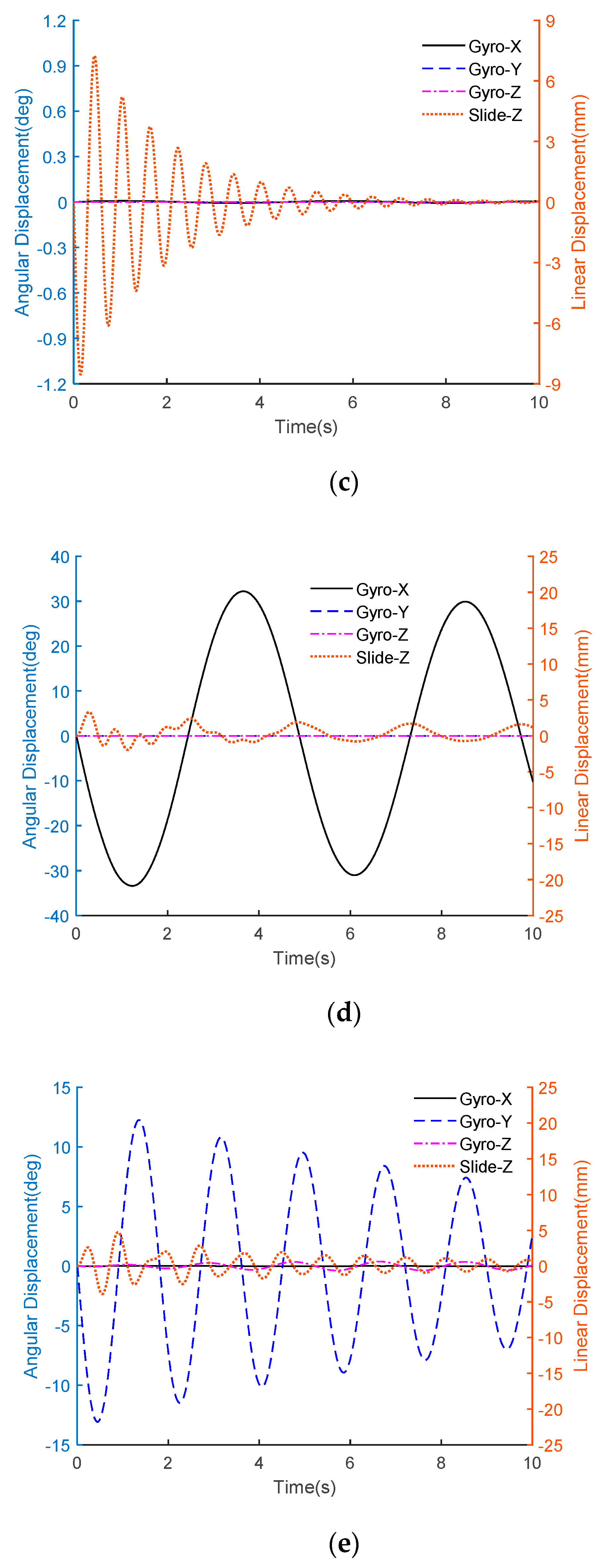
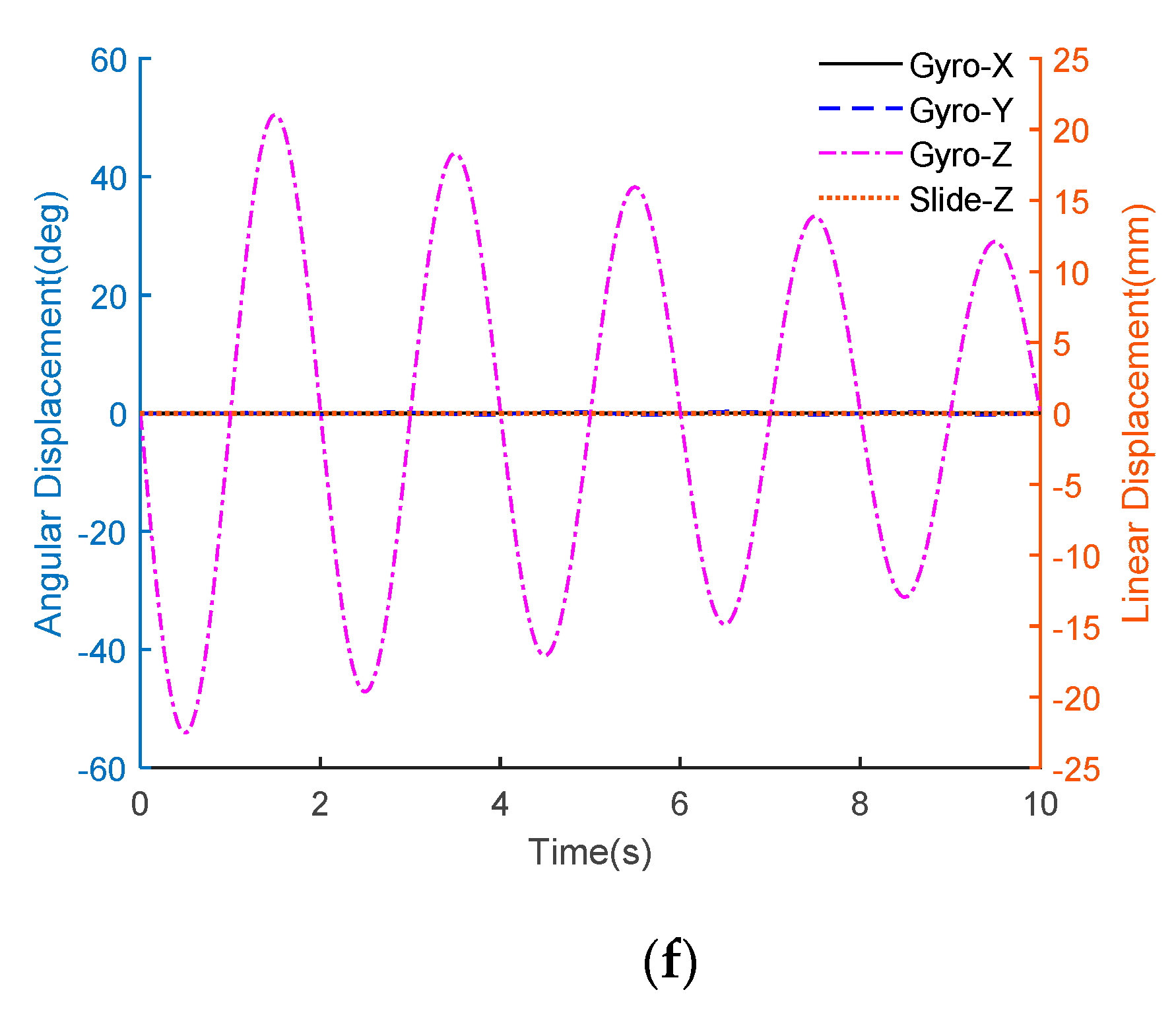
The bionic docking mechanism is expected to have the capability of both buffering and unloading momentum in any direction. In this section, as shown in Figure 15, six unidirectional collision forces, i.e., (a) Fx namely the X–line force, (b) Mx namely X–angle torque, (c) Fy namely Y–line force, (d) My namely the Y–angle torque, (e) Fz namely the Z–line force and (f) Mz namely the Z–angle torque are sequentially applied at the end of the bionic docking mechanism, respectively. The unloading and buffer effect can be judged by measuring the spring deformations in the joints to verify the soft contact machine–processed as shown in Figure 4.
The simulation parameters are as follows: the flexible parameters of the bionic docking mechanism are shown in Table 6, the single–dimensional force or torque applied at the end of the bionic docking mechanism is 100 N or 100 N m, and the impact time is 0.01 s, and the simulation time is 10 s.
As shown in Figure 16, the numerical simulation results in MATLAB are carried out comparatively. The vibration displacements of each joint of the bionic docking mechanism are given respectively. It can be seen that when the bionic docking mechanism is only subjected to X–line or Y–angle collision, only the vibration displacement of the Gyro–Y joint is produced as shown in Figure 16a,e, and when the bionic docking mechanism is only subjected to Y–line or X–angle collision, only the vibration displacement of the Gyro–X joint is produced as shown in Figure 16b or Figure 16d. When the bionic docking mechanism is only subjected to the Z–angle collision, only the vibration displacement of the Gyro–Z joint is produced as shown in Figure 16f, and when the bionic docking mechanism is only subjected to a single Z–line collision, only the vibration displacement of the Slide–Z joint is produced as shown in Figure 16c. Moreover, all the vibration displacements of the bionic docking mechanisms can converge under the action of damping, and the soft contact machine–processed proposed in Figure 4 can be verified.
6. Docking Collision Experiment
As shown in Figure 17, The space target docking collision model of spaceborne capture mechanism with the bionic docking mechanism is established in Adams, and then the space target docking collision experiment is carried out in this section. The flow chart of Adams simulation is shown in Figure 18.
In this section, the space target collision model in Adams is simulated under the conditions of rigidity, damping 1 and damping 2, and the angular velocity and linear velocity of the free–floating base and the vibration displacement of each joint is obtained to verify the effectiveness of the bionic docking mechanism in buffering and unloading the spatially six–dimensional collision caused by space target docking.
The specific simulation parameters are as follows: the dynamics parameters of the space target are shown in Table 7, the initial position related to the end of the bionic docking mechanism is [200, 200, 200] mm; The collision parameters in Adams are shown in Table 8; The stiffness of the bionic docking mechanism can be obtained from Section 5.1, the damping parameters are shown in Table 9, and the simulation time is 10 s.
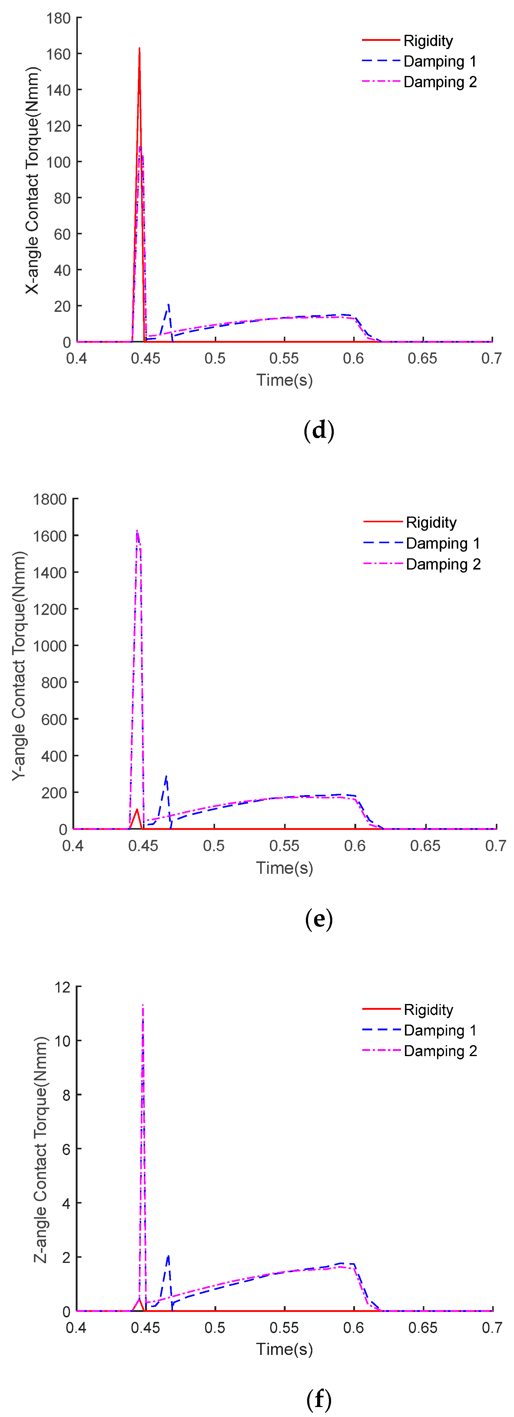
The spatially six–dimensional collision (contact forces and torques) caused by space target docking are shown in Figure 19. Figure 19a–c are the X–line, Y–line and Z–line contact force, Figure 19d–f are the X–angle, Y–angle and Z–angle contact torque under the docking collision. It can be seen that the contact time of the docking collision under rigidity condition is about 0.01 s, while the contact time of space target docking collision under the conditions of damping 1 and damping 2 is about 0.18 s. It can be seen that the bionic docking mechanism can prolong the contact time of space target docking collision to provide sufficient response time for the spatial capture.
As shown in Figure 20, under the docking collision, the linear velocity and angular velocity of the free–floating base will suddenly change under the condition of rigidity. Under the condition of damping 1, the linear velocity and angular velocity of the free–floating do not change suddenly, but there is a long–term oscillation. Under the condition of damping 2, the linear velocity and angular velocity of the free–floating base can converge in 6 s. The simulation results indicate that the controllable MR dampers loaded by the bionic docking mechanism can absorb the docking collision, and has the ability to buffer and unload the space six–dimensional collision caused by space target docking to avoid the instability of the free–floating base.
Figure 21 shows the vibration displacements of each joint of the bionic docking mechanism under the conditions of damping 1 and damping 2 under the docking collision. It can be obtained that with the increase of damping coefficients, the vibration peak of each joint decreases and does not exceed the limited amplitude of the each joint, which illustrates the effectiveness of the optimization simulation in Section 5.1. Under the condition of damping 2, all the vibration displacements can be stabilized, in which the vibration displacement of the Gyro–X joint is stabilized in about 7 s, the vibration displacement of the Gyro–Y joint is stabilized in about 5 s, and the vibration displacement of the Gyro–Z joint is stabilized in about 4 s, while the vibration displacement of Slide–Z joint is stabilized in about 7 s. The simulation results indicate that the MR dampers can stabilize the displacements at each DOF of the bionic docking mechanism under docking collision.
Through the analysis of the angular velocity and linear velocity of the free–floating base under the space target docking collision, it is verified that the bionic docking mechanism has the ability to buffer and unload the six–dimensional collision caused by space target docking, that is, avoid free–floating base instability. Through the analysis of the vibration displacements, the rationality of the optimization scheme based on Section 4 is further verified.
7. Conclusions
(1) A bionic docking mechanism for space target acquisition, imitating wrist movement, is proposed to realize the buffering and unloading of six–dimensional spatial collisions through flexible rotating and linear components.
(2) A dynamic model of the bionic docking mechanism in space docking using the Kane method is proposed, and the results of dynamic analysis of the optimization strategy show that the optimization of the stiffness of the bionic docking mechanism can avoid the instability of the base.
(3) Particle swarm optimization (PSO) was used to realize the stiffness optimization of the bionic docking mechanism, that is, the optimal stiffness coefficients are 30 in Gyro–X joint, 193 in Gyro–Y joint, 43 in Gyro–Z joint, and 0.85 in Slide–Z joint. And the simulation results indicate that the soft contact machine–processed proposed can be verified.
(4) Through the docking collision experiment of the spaceborne capture mechanism with the bionic docking mechanism, the simulation results indicate that the proposed bionic docking mechanism can prolong the collision time from 0.01 s to 0.18 s to win time for space acquisition, avoid velocity mutation of the free–floating base, and stabilize the bionic docking mechanism by damping vibration absorption; that is, the effectiveness of the bionic docking mechanism can be verified in buffering and loading the spatially six–dimensional collision caused by space target docking. The stabilization control of the spaceborne capture mechanism by damping optimization with the bionic docking mechanism could be a direction for future research.
Author Contributions
Conceptualization, S.X. and M.C.; methodology, S.X.; software, S.X.; validation, S.X., M.C. and H.S.; formal analysis, S.X.; investigation, M.C.; resources, S.X.; data curation, S.X.; writing—original draft preparation, S.X.; writing—review and editing, M.C.; visualization, H.S.; supervision, H.S.; project administration, M.C.; funding acquisition, M.C. All authors have read and agreed to the published version of the manuscript.
Funding
This work is partially supported by the National Natural Science Foundation of China (Grant No. 51875046) and Natural Science Foundation of Beijing Municipality (Grant No. 3202021). The authors would like to thank anonymous reviewers for their valuable comments to improve the quality of this paper.
Institutional Review Board Statement
Not applicable.
Informed Consent Statement
Not applicable.
Conflicts of Interest
The authors declare no conflict of interest.
References
- Zhang, C.; Bai, H. Space docking mechanism technology of spacecraft. Sci. Sin. 2014, 44, 20. [Google Scholar] [CrossRef]
- Wang, B.; Zhuang, Y.; Liu, P.; Wang, N.; Han, R.; Zhu, J. Review of Spacecraft Electromagnetic Docking Technology Development. Spacecr. Eng. 2018, 27, 92–101. [Google Scholar]
- Feng, F.; Tang, L.N.; Xu, J.F.; Liu, H.; Liu, Y.W. A review of the end–effector of large space manipulator with capabilities of misalignment tolerance and soft capture. Sci. China 2016, 59, 1621. [Google Scholar] [CrossRef]
- Kang, Y.; Zhou, H.; Ma, S.J.; Gao, B.; Tan, L. Review of Spacecraft Exposed Payload Adapter Technology. Spacecr. Eng. 2019, 28, 104–111. [Google Scholar]
- Fa, A.; Ou, M.A.; Kp, B.; Su, C. A review of space robotics technologies for on–orbit servicing. Prog. Aerosp. Sci. 2014, 68, 1–26. [Google Scholar]
- Feng, F.; Liu, Y.W.; Liu, H.; Cai, H.G. Development of space end–effector with capabilities of misalignment tolerance and soft capture based on tendon–sheath transmission system. J. Cent. South Univ. 2013, 20, 3015–3030. [Google Scholar]
- Liu, Y.; Yao, Y.A.; He, Y.Y. Design and research of topological 3–RSR polyhedron docking mechanism. Manned Spacefl. 2018, 24, 61–66. [Google Scholar]
- Li, L.Q.; Zhang, G.Y.; Bai, H.M.; Chen, M.; Fan, Z. Design and Mechanical Analysis for a Three–Arm Non–Cooperative Target Satellite Docking Mechanism. Aerosp. Shanghai 2015, 32, 5–11. [Google Scholar]
- Zhang, M.; Ye, M.; Liu, P.; Qi, Z.; Hong, Z.; Wang, M.; Chen, G.H.; Deng, F.Y.; Zhang, L.P. The Demonstrations of Flux Pinning for Space Docking of CubeSat Sized Spacecraft in Simulated Microgravity Conditions. IEEE Trans. Appl. Supercond. 2019, 6, 1. [Google Scholar]
- Sohal, S.S.; Sebastian, B.; Ben–Tzvi, P. Autonomous Docking of Hybrid–Wheeled Modular Robots With an Integrated Active Genderless Docking Mechanism. ASME J. Mech. Rob. 2021, 14, 011010. [Google Scholar]
- Shi, K.K.; Sun, Z.W.; Liu, C.; Ye, D. Dynamics modeling and simulation of space electromagnetic docking for CubeSat. In Proceedings of the 2017 8th International Conference on Mechanical and Aerospace Engineering (ICMAE), Prague, Czech Republic, 22–25 July 2017. [Google Scholar]
- Zhuang, Y.; Xie, Z.; Wang, B.; Wang, W.; Li, W.; Wang, Y. Design and Analysis for a Novel Docking Mechanism with T–type Locking Structure in Space. In Proceedings of the 2019 IEEE 9th Annual International Conference on CYBER Technology in Automation, Control, and Intelligent Systems (CYBER), Suzhou, China, 29 July–1 August 2019. [Google Scholar]
- Chen, C.Z.; Nie, H.; Chen, J.B.; Wang, X.T. Study on Movement Space in Capture System with Low Impact Docking Mechanism. J. Astronaut. 2014, 35, 1000–1006. [Google Scholar]
- Han, W.; Jiang, Z.J.; Huang, Y.Y.; Chen, X.Q. Designing of Conical Surface Configuration for the Probe–cone Docking Mechanism Facing to Mini–Spacecraft. Chin. J. Space Sci. 2019, 39, 228–232. [Google Scholar]
- Moubarak, P.M.; Ben–Tzvi, P. On the Dual–Rod Slider Rocker Mechanism and Its Applications to Tristate Rigid Active Docking. ASME J. Mech. Rob. 2013, 5, 011010. [Google Scholar]
- Zhang, M.; Yu, D.; Deng, Z.; Liu, P.; Niu, J.; Yu, Z.; Liu, Y.; Xu, X. The mechanical characteristics and control of high temperature superconducting magnetic docking mechanism. AIP Adv. 2021, 11, 055208. [Google Scholar] [CrossRef]
- Cao, B.; Yuan, J.J.; Zhang, T.; Weng, S.T.; Yao, J. FPGA–Based Docking Mechanism Prototype Docking Ring Control Research. Procedia Comput. Sci. 2020, 166, 252–257. [Google Scholar] [CrossRef]
- Xu, C.T.; Li, J.G.; Wang, P.; Xu, Z.D. A Study of Transmission Error Modeling and Preload Compensation for the Cable–Driven Sheaves Used in Space Docking Locks. J. Mech. 2020, 36, N9–N20. [Google Scholar] [CrossRef]
- Zhang, Y.; Shao, J.; Wang, P.; Li, J.; Zhang, P. Non–Fragile Reliable Control Law with the D–Stability of a Claw–Shaped Docking Mechanism Based on Kinetic Analysis. J. Comput. Theor. Nanosci. 2016, 13, 1584–1592. [Google Scholar] [CrossRef]
- Olivieri, L.; Francesconi, A. Design and test of a semiandrogynous docking mechanism for small satellites. Acta Astronaut. 2016, 122, 219–230. [Google Scholar] [CrossRef]
- Li, L.Q.; Shao, G.B.; Zhou, D.K.; Liu, W.; Wang, J. Design and analysis of a long–stroke and miniaturized docking mechanism. Manned Spacefl. 2016, 22, 758–765. [Google Scholar]
- Zhang, X.; Huang, Y.Y.; Chen, X.Q. Analysis and design of parameters in soft docking of micro/small satellites. Sci. China Inf. Sci. 2017, 60, 51–64. [Google Scholar] [CrossRef]
- Zhang, Y.W.; Zhu, Y.W.; Zhu, H.K. Spacecraft self– and soft–docking via coupled actuation of magnetic fields. In Proceedings of the 2020 39th Chinese Control Conference (CCC), Shenyang, China, 27–29 July 2020. [Google Scholar]
- Wei, Q.; Liu, Z.; Wang, Y.; Shao, L. Impedance Control of Space Flexible Manipulator System Assisted Docking of Space Station. Chin. Space Sci. Technol. 2014, 34, 57–64. [Google Scholar]
- Cong, P.C.; Zhang, X. Preimpact configuration analysis of a dual–arm space manipulator with a prismatic joint for capturing an object. Robotica 2013, 31, 853–860. [Google Scholar] [CrossRef]
- Oki, T.; Nakanishi, H.; Yoshida, K. Time–optimal manipulator control for management of angular momentum distribution during the capture of a tumbling target. Adv. Robot. 2010, 24, 441–466. [Google Scholar] [CrossRef]
- Hu, J.; Wang, T. Pre–Impact Configuration Designing of a Robot Manipulator for Impact Minimization. ASME J. Mech. Rob. 2017, 9, 031010. [Google Scholar]
- Gan, D.; Tsagarakis, N.G.; Dai, J.S.; Caldwell, D.G.; Seneviratne, L. Stiffness Design for a Spatial Three Degrees of Freedom Serial Compliant Manipulator Based on Impact Configuration Decomposition. ASME J. Mech. Rob. 2013, 5, 011002. [Google Scholar] [CrossRef]
- Hu, J.; Wang, T. Minimum Base Attitude Disturbance Planning for a Space Robot During Target Capture. ASME J. Mech. Rob. 2018, 10, 051002. [Google Scholar] [CrossRef]
- Song, S.; She, Y.; Wang, J.; Su, H. Toward Tradeoff Between Impact Force Reduction and Maximum Safe Speed: Dynamic Parameter Optimization of Variable Stiffness Robots. ASME J. Mech. Rob. 2020, 12, 054503. [Google Scholar] [CrossRef]
- Guo, W.H.; Wang, T.S. Pre–impact configuration optimization for a space robot capturing target satellite. J. Astronaut. 2015, 36, 390–396. [Google Scholar]
- Chen, X.; Qin, S. Motion Planning for dual–arm space robot towards capturing target satellite and keeping the base inertially fixed. IEEE Access 2018, 6, 26292–26306. [Google Scholar]
- Xu, W.; Yan, L.; Hu, Z.; Liang, B. Area–oriented coordinated trajectory planning of dual–arm space robot for capturing a tumbling target. Chin. J. Aeronaut. 2019, 32, 2151–2163. [Google Scholar] [CrossRef]
- Larouche, B.P.; Zhu, Z.H. Autonomous robotic capture of non–cooperative target using visual servoing and motion predictive control. Auton. Robot. 2014, 37, 157–167. [Google Scholar] [CrossRef]
- Zhang, L.; Jia, Q.X.; Chen, G. Pre–impact trajectory planning for minimizing base attitude disturbance in space manipulator systems for a capture task. Chin. J. Aeronaut. 2015, 28, 1199–1208. [Google Scholar]
- Chu, M.; Zhang, X.; Xu, S.; Yu, X.; Wang, D. Modeling and stabilization control for space–borne series–wound capturing mechanism with multi–stage damping. Mech. Syst. Signal Process. 2020, 145, 106973. [Google Scholar]
- Nguyen, H.; Thai, C.; Sharf, I. Capture of spinning target with space manipulator using magneto rheological damper. In Proceedings of the AIAA Guidance, Navigation, and Control Conference, Toronto, ON, Canada, 2–5 August 2010; pp. 1–12. [Google Scholar]
- Yu, Z.W.; Liu, X.F.; Cai, G.P. Dynamics modeling and control of a 6–DOF space robot with flexible panels for capturing a free–floating target. Acta Astronaut. 2016, 128, 560–572. [Google Scholar]
- Balamurugan, L.; Jancirani, J.; Eltantawie, M.A. Generalized magnetorheological (MR) damper model and its application in semi–active control of vehicle suspension system. Int. J. Automot. Technol. 2014, 15, 419–427. [Google Scholar]
- Bian, Y.; Gao, Z.; Lv, X.; Fan, M. Theoretical and experimental study on vibration control of flexible manipulator based on internal resonance. J. Vib. Control. 2018, 24, 3321–3337. [Google Scholar]
- Xin, P.; Rong, J.; Yang, Y.; Xiang, D.; Xiang, Y. Trajectory planning with residual vibration suppression for space manipulator based on particle swarm optimization algorithm. Adv. Mech. Eng. 2017, 9, 1–16. [Google Scholar] [CrossRef] [Green Version]
- Zawidzki, M.; Szklarski, J. Transformations of Arm–Z modular manipulator with Particle Swarm Optimi–zation. Adv. Eng. Softw. 2018, 126, 147–160. [Google Scholar]
- Marinaki, M.; Marinakis, Y.; Stavroulakis, G.E. Vibration control of beams with piezoelectric sensors and actuators using particle swarm optimization. Expert Syst. Appl. 2011, 38, 6872–6883. [Google Scholar]
- Farshidianfar, A.; Saghafi, A.; Kalami, S.M.; Saghafi, I. Active vibration isolation of machinery and sensitive equipment using H ∞ control criterion and particle swarm optimization method. Meccanica 2012, 47, 437–453. [Google Scholar] [CrossRef]
- Huang, W.; Xu, J.; Zhu, D.Y.; Wu, Y.L.; Lu, J.W.; Lu, K.L. Semi–active Vibration Control Using a Magneto Rheological (MR) Damper with Particle Swarm Optimization. Arab. J. Sci. Eng. 2015, 38, 6872–6883. [Google Scholar] [CrossRef]
Figure 1.
3D model of the bionic docking mechanism.

Figure 2.
Generalized model of the bionic docking mechanism in space docking.

Figure 3.
Over structure of the bionic docking mechanism; (a) Gyro–structure assembly; (b) Sliding–structure assembly; 1. Encorder; 2. Rotating MR damper; 3. Gyro frame 3; 4. Sliding frame 1; 5. Electromagnetic clutch; 6. Torsion spring; 7. Gyro frame 1; 8. Gyro frame 2; 9. Linear spring; 10. Electromagnetic braking slide; 11. Linear MR damper; 12. Slider; 13. Sliding frame 1; 14. Linear displacement sensor.

Figure 4.
Transmission schematic of the X–line and Y–line collision.

Figure 5.
Model of the bionic docking mechanism in space docking.

Figure 6.
Modeling of particle swarm optimization.

Figure 7.
Flow chart of stiffness optimization based on PSO.

Figure 8.
Collision diagram of spatially six–dimensional collision.

Figure 9.
Fitness values of 100 numerical simulations.

Figure 10.
Torsion/Linear spring stiffness coefficients of 100 numerical simulations.

Figure 11.
Gyro–X joint vibration displacements under min and max fitness.

Figure 12.
Gyro–Y joint vibration displacements under min and max fitness.

Figure 13.
Gyro–Z joint vibration displacements under min and max fitness.

Figure 14.
Slide–Z joint vibration displacements under min and max fitness.

Figure 15.
Collision diagram of soft contact machine–processed simulation.

Figure 16.
Vibration displacement under six unidirectional collision; (a) Vibration displacements under X–line collision; (b) Vibration displacements under Y–line collision; (c) Vibration displacements under Z–line collision; (d) Vibration displacement under X–angle collision; (e) Vibration displacement under Y–angle collision; (f) Vibration displacement under Z–angle collision.


Figure 17.
Space target docking collision model.

Figure 18.
Flow chart of Adams simulation.

Figure 19.
Spatially six–dimensional collision caused by space target docking; (a) X–line contact force; (b) Y–line contact force; (c) Z–line contact force; (d) X–angle contact torque; (e) Y–angle contact torque; (f) Z–angle contact torque.
Figure 19.
Spatially six–dimensional collision caused by space target docking; (a) X–line contact force; (b) Y–line contact force; (c) Z–line contact force; (d) X–angle contact torque; (e) Y–angle contact torque; (f) Z–angle contact torque.


Figure 20.
Linear velocity and angular velocity of the base under space target docking collision; (a) X–line velocity of base; (b) Y–line velocity of base; (c) Z–line velocity of base; (d) X–angle velocity of base; (e) Y–angle velocity of base; (f) Z–angle velocity of base.
Figure 20.
Linear velocity and angular velocity of the base under space target docking collision; (a) X–line velocity of base; (b) Y–line velocity of base; (c) Z–line velocity of base; (d) X–angle velocity of base; (e) Y–angle velocity of base; (f) Z–angle velocity of base.


Figure 21.
Vibration displacements of each joint of the bionic docking mechanism; (a) Vibration displacements of under Damping 1; (b) Vibration displacements of under Damping 2.
Figure 21.
Vibration displacements of each joint of the bionic docking mechanism; (a) Vibration displacements of under Damping 1; (b) Vibration displacements of under Damping 2.


Table 1.
Limited amplitude and control amplitude of each DOF.
| Type | Gyro–X | Gyro–Y | Gyro–Z | Slide–Z |
|---|---|---|---|---|
| Limited Amplitude | 70.0 | 30.0 | 90.0 | 25.0 |
| Control Amplitude | 50.0 | 20.0 | 70.0 | 17.0 |
| Unit | deg | mm | ||
Table 2.
Model parameters of space–capture mechanism.
| k | mk/kg | Ik/kg·m2 | dk/m | rk/m | ||
|---|---|---|---|---|---|---|
| X | Y | Z | ||||
| 1 | 200 | 55 | 55 | 50 | 6.71 | 1.51 |
| 2 | 1.9 | 0.03 | 0.005 | 0.03 | 0 | 0 |
| 3 | 1.7 | 0.015 | 0.01 | 0.005 | 0 | 0 |
| 4 | 1.7 | 0.02 | 0.02 | 0.004 | 0.21 | 0.21 |
| 5 | 8 | 0.5 | 0.5 | 0.25 | 0.22 | 0.13 |
Table 3.
Initial damping of the bionic docking mechanism.
| Type | Unit | Value |
|---|---|---|
| Gyro–X | 0.2 | |
| Gyro–Y | 0.2 | |
| Gyro–Z | 0.2 | |
| Slide–Z | 0.00001 |
Table 4.
Stiffness of the bionic docking mechanism.
| Value | Gyro–X | Gyro–X | Gyro–X | Slide–Z |
|---|---|---|---|---|
| Min Fitness | 29.4 | 193 | 42.7 | 0.850 |
| Max Fitness | 43.4 | 137 | 84.3 | 0.945 |
| Unit | ||||
Table 5.
Vibration Peak of the bionic docking mechanism.
| Peak | Gyro–X | Gyro–X | Gyro–X | Slide–Z |
|---|---|---|---|---|
| Min Fitness | 50.5 | 29.5 | 78.9 | 21.4 |
| Max Fitness | 41.0 | 26.2 | 54.1 | 16.2 |
| Unit | deg | mm | ||
Table 6.
Flexible parameters of the bionic docking mechanism.
| Type | Stiffness | Damping |
|---|---|---|
| Gyro–X | 30 | 0.2 |
| Gyro–Y | 193 | 0.2 |
| Gyro–Z | 43 | 0.2 |
| Slide–Z | 0.85 | 0.00001 |
Table 7.
Space target parameters.
| Value | Linear Velocity | Angular Velocity | Inertia | Mass |
|---|---|---|---|---|
| X | 500 | 30 | 50,000 | 2 |
| Y | 500 | 30 | 50,000 | |
| Z | 500 | 30 | 50,000 | |
| Unit | mm/s | deg/s | kg |
Table 8.
Collision model parameters.
| Type | Description | Unit | Value |
|---|---|---|---|
| Normal Force | Stiffness | N/mm | 100,000 |
| Force index | / | 2.2 | |
| Damping | 10 | ||
| Penetration depth | mm | 0.1 | |
| Friction | Static friction coefficient | / | 0.3 |
| Dynamic friction coefficient | / | 0.1 | |
| Static translation velocity | mm/s | 100 | |
| Friction translation velocity | mm/s | 1000 |
Table 9.
Damping parameters of the bionic docking mechanism.
| Type | Gyro–X | Gyro–Y | Gyro–Z | Slide–Z |
|---|---|---|---|---|
| Damping 1 | 0.2 | 0.2 | 0.2 | 0.00001 |
| Damping 2 | 17.50 | 17.50 | 17.50 | 0.01 |
| Unit | ||||
Publisher’s Note: MDPI stays neutral with regard to jurisdictional claims in published maps and institutional affiliations. |
© 2021 by the authors. Licensee MDPI, Basel, Switzerland. This article is an open access article distributed under the terms and conditions of the Creative Commons Attribution (CC BY) license (https://creativecommons.org/licenses/by/4.0/).
Share and Cite
MDPI and ACS Style
Xu, S.; Chu, M.; Sun, H. Design and Stiffness Optimization of Bionic Docking Mechanism for Space Target Acquisition. Appl. Sci. 2021, 11, 10278. https://0-doi-org.brum.beds.ac.uk/10.3390/app112110278
AMA Style
Xu S, Chu M, Sun H. Design and Stiffness Optimization of Bionic Docking Mechanism for Space Target Acquisition. Applied Sciences. 2021; 11(21):10278. https://0-doi-org.brum.beds.ac.uk/10.3390/app112110278
Chicago/Turabian StyleXu, Sheng, Ming Chu, and Hanxu Sun. 2021. "Design and Stiffness Optimization of Bionic Docking Mechanism for Space Target Acquisition" Applied Sciences 11, no. 21: 10278. https://0-doi-org.brum.beds.ac.uk/10.3390/app112110278
Note that from the first issue of 2016, this journal uses article numbers instead of page numbers. See further details here.