
The Vehicle Routing Problem: State-of-the-Art Classification and Review


Department of Industrial Engineering and Engineering Management, Integration and Collaboration Laboratory, National Tsing Hua University, Hsinchu 30013, Taiwan
*
Author to whom correspondence should be addressed.
Appl. Sci. 2021, 11(21), 10295; https://0-doi-org.brum.beds.ac.uk/10.3390/app112110295
Submission received: 28 September 2021
/
Revised: 21 October 2021
/
Accepted: 28 October 2021
/
Published: 2 November 2021
(This article belongs to the Special Issue Smart Manufacturing Networks for Industry 4.0)
Abstract
:Transportation planning has been established as a key topic in the literature and social production practices. An increasing number of researchers are studying vehicle routing problems (VRPs) and their variants considering real-life applications and scenarios. Furthermore, with the rapid growth in the processing speed and memory capacity of computers, various algorithms can be used to solve increasingly complex instances of VRPs. In this study, we analyzed recent literature published between 2019 and August of 2021 using a taxonomic framework. We reviewed recent research according to models and solutions, and divided models into three categories of customer-related, vehicle-related, and depot-related models. We classified solution algorithms into exact, heuristic, and meta-heuristic algorithms. The main contribution of our study is a classification table that is available online as Appendix A. This classification table should enable future researchers to find relevant literature easily and provide readers with recent trends and solution methodologies in the field of VRPs and some well-known variants.
1. Introduction
Problems related to the distribution of goods between warehouses and customers are generally considered as vehicle routing problems (VRPs). The VRP was first proposed by Dantzig and Ramser [1] in 1959 to model how a fleet of homogeneous trucks could serve the demand for oil from a number of gas stations from a central hub with a minimum travel distance. Five years later, Clarke and Wright [2] added more practical restrictions to VRPs in which the delivery of goods to each customer must occur within a set of bounds. This type of problem model became known as the VRP with time windows (VRPTW), which is one of the most widely studied topics in the field of operations research [3].
However, current VRP models differ significantly from those introduced by Dantzig and Ramser [1] and Clarke and Wright [2], because they aim to incorporate real-world complexities. Because VRPs are some of the most critical challenges faced by logistics companies, an increasing amount of research is focusing on VRPs. Several surveys and taxonomies for VRPs can be found in [3,4,5,6] ((Eksioglu et al. (2009); Braekers et al. (2016); Elshaer and Awad (2020); Konstantakopoulos et al. (2020)) and in many other books or book chapters [7,8,9,10] ((Cordeau et al. (2007); Golden et al. (2008); Toth and Vigo (2014)); Nalepa (2019)).
Solving VRPs is computationally expensive and categorized as NP-hard [11], because real-world problems involve complex constraints such as time windows, time-dependent travel times (reflecting traffic congestion), multiple depots, and heterogeneous fleets. These features introduce significant complexity and have dramatically evolved the VRP research landscape.
The processing speed and memory capacity of computers has grown rapidly, enabling the processing of increasingly complex instances of VRPs and widespread application of logistics distribution scenarios. The number of VRP solution methods introduced in the academic literature has grown rapidly over the past few decades. According to Eksioglu et al. [4], the VRP represents an evolving field of operations research that has been growing exponentially at a rate of 6% per year, which makes it difficult to keep track of developments in the field and obtain a clear overview of which variants and solution methods are relatively novel.
The VRP family can be considered as two combinatorial senses: (1) the number of possible solutions, which grow exponentially with computer science and algorithm design; and (2) the number of conceivable problem variants, which also grow exponentially with a variety of problem attributes [12]. This survey classifies the academic literature on VRPs from the perspective of solution methodologies, as well as the detailed characteristics of VRPs. Because we base our classification on the taxonomy presented in [4], we restrict our analysis to articles published between 2019 and August of 2021. Therefore, we do not intend to provide an exhaustive overview of VRP literature. To the best of our knowledge, this article provides the first structured classification of recent VRP literature based on solution and problem attributes.
The main contribution of our paper is a classification table that is available online as Appendix A. This classification table should enable future researchers to find relevant literature easily by eliminating or selecting characteristics in the taxonomy, leaving only articles tailored to their interests. The main objective of this work is to provide readers with recent trends and solution methodologies in the field of VRPs and some well-known variants. This survey is expected to help future researchers identify a problem domain and promising topics for research.
2. Scope of the Survey
We analyzed recent literature published between 2019 and August of 2021 using a taxonomic framework. Classification is followed by a survey that uses the taxonomy to evaluate trends in the field and identify which articles contribute to these trends. We restricted the reviewed literature to the following features: only relevant articles published in English-language journals were considered, meaning books, conference proceedings, and dissertations were excluded.
To extract the most relevant literature and keep the number of articles manageable, the following search strategy was applied. First, only articles containing ‘‘vehicle routing” as title words or keywords were selected. Second, the search was limited to articles that were extended by highly cited articles published in any ranked journal (Google Scholar top 20), excluding review papers. For papers published in 2021, which are too recent to have cite ranking, we selected the top five pages from Google Scholar, each of which had 10 cited articles, as well as two review papers written by Moghdani et al. [13] and Asghari and Al-e (2021). Third, the abstracts of selected articles were read to determine their relevance to the subject.
This search strategy resulted in a final set of 88 articles. Although this selection is not exhaustive, it contains the majority of recent articles on VRPs and can be considered as representative of the field.
3. VRP and Its Variants
3.1. VRP
In addition to the classical VRP, several variants have also been studied. Capacitated VRP (CVRP), VRPTW, VRP with heterogeneous fleets (HFVRP), time-dependent VRP (TDVRP), and multi-depot VRP (MDVRP) are some of these variants. The classical VRP can be described as follows. Let be a graph, where , where is the node set representing customers to be served and is the depot. Each customer is characterized by a demand . is the arc set (subscript indicates sequence) linking nodes i and j with a distance . Let denote the vehicle set, where each vehicle has a maximum load capacity , meaning the total load of vehicle m cannot exceed the maximum load capacity . To reflect a real distribution scenario accurately, different features are considered according to the settings of heterogeneous models. The goal of the VRP is to derive optimal vehicle routes such that each customer is visited exactly once by one vehicle and each vehicle starts and ends its route at the depot. The following assumptions are adopted:
- The depot has a demand equal to zero.
- Each customer location is serviced by only one vehicle.
- Each customer’s demand is indivisible.
- Each vehicle shall not exceed its maximum load capacity capm.
- Each vehicle starts and ends its route at the depot.
- Customer demand, distribution distances between customers, and delivery costs are known.
Traditional logistics models focus on minimizing the total cost of a network. This is where the concept of the VRP is best applied. We follow this concept and add the fixed cost of a vehicle, which represents rent cost or operating costs, to the total cost to minimize the total number of vehicles. We also include the variable cost of delivery using each type of vehicle to optimize vehicle scheduling. Additional constraints appear in the target calculation in the form of penalty functions to enforce vehicle limit constraints. The objective of minimizing the total cost is defined as follows:
subject to the following constraints:
Routing:
Demand and capacities:
The objective function in Equation (1) is the total cost, which includes the fixed cost and variable cost. Constraint (2) states that each vehicle should return to the depot, where the subscript is zero. Constraint (3) ensures that each node can only be visited once in a route. Constraint (4) states that, if a vehicle arrives at a node, it must leave that node, thereby ensuring route continuity. Constraints (5) and (6) impose restrictions on the amounts of demand and capacity. Constraint (7) defines the maximum number of available vehicles vehm.
3.2. VRP Variants
Practical requirements and new challenges require extensive definitions and formulations of the VRP. For example, distance, driver working hours, time windows, traffic conditions, and so on can all arise in real-world VRPs and enrich the definition and applications of VRPs. This chapter provides an overview of recent research on different models for vehicle routing. The main goal of this chapter is to present an overview of vehicle routing and scheduling areas while discussing several real-world applications.
Some features of VRPs are summarized in Table 4 based on the research by Eksioglu et al. [4]. Other variants have also been studied beyond the classical VRP. These variants include the influence of time factors, time windows of customers, maximum operating time of vehicles, differing delivery times caused by varying traffic conditions, varying characteristics of vehicles, varying capacities, varying speeds, and new types of electric vehicles. By referring to the taxonomy of [4], we divided models into three main categories: customer-related, vehicle-related, and depot-related models, which is the most important issue to represent the difference in real delivery problems. These categories have representative model features that are sorted in the tables below according to the year as shown in Table 5, Table 6 and Table 7.
The objectives of VRPs can also be diversified according to different stakeholder requirements. The traditional objective of the standard VRP is to minimize a cost function, which is considered to be the total distance traveled by all vehicles. However, recent studies have focused on various negative externalities of transportation, including carbon emissions and duration. For an objective discussion, we classified single and multiple objectives according to the diversity of objectives and then listed the objectives used in different studies. The papers with the same numbers as those in Table 2, Table 3 and Table 4 are listed in Table 8, Table 9 and Table 10. Additionally, we discussed the test instances used in different studies.
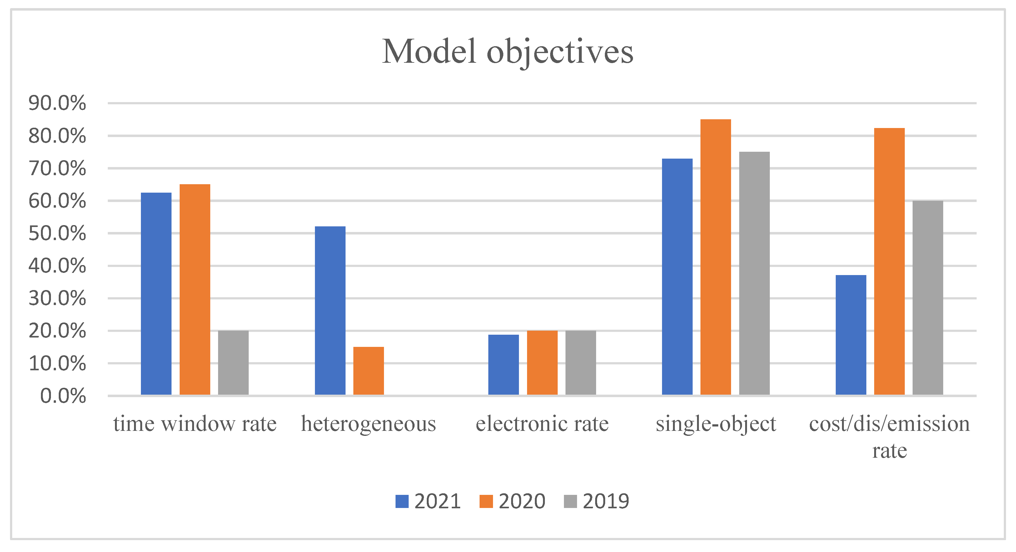
As shown in the tables above, there are different main model objectives for different years. The results are summarized in Figure 1.
One can see that the time window still occupies a large proportion of model objectives and is the mainstream of current research on the VRP and its variants. This trend is closely related to the concept of the “to C” distribution, where customers focus on service satisfaction. There have been various extensions of the VRP, including the VRPTW and time-dependent problems such as those discussed in [17,24,41,75,89]. Additional research has focused on heterogeneous vehicle problems that are closely related to real-life vehicle applications. With the increasing focus on environmental protection, electric vehicle distribution has also gradually become a mainstream research topic. Relevant research can be found in [49,72,81,89,116]. Single-objective models still occupy a certain research space, where the objective value setting is still largely based on cost metrics (e.g., cost, distance, and CO2 emission). However, unlike cost metrics in past research, the costs in the current single-objective problem research tend to be compound costs representing actual delivery costs.
4. Solutions for VRPs
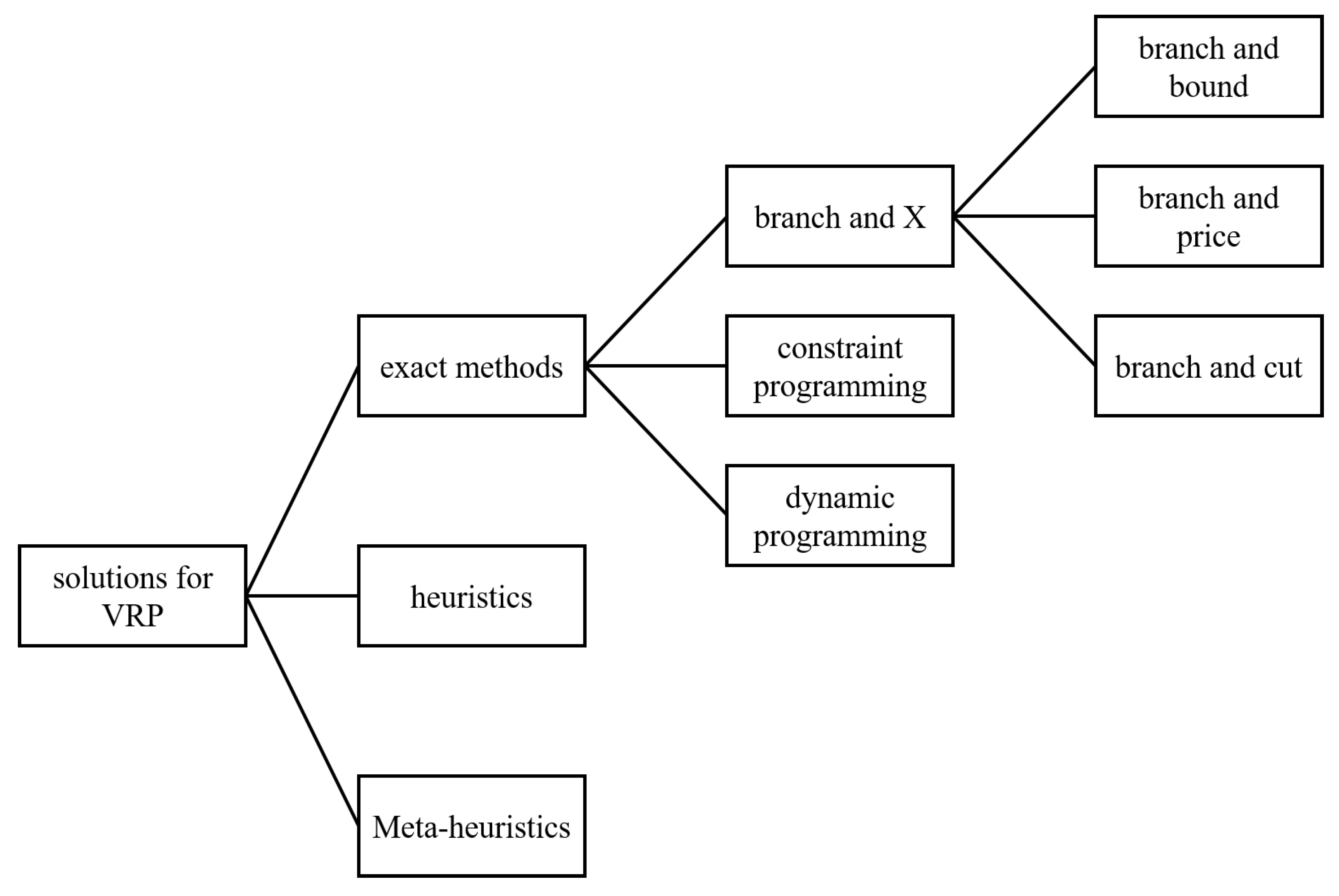
Because real-world problems involve complex constraints, advanced algorithms are required to solve VRPs in complicated and constantly changing environments. The number of customers and vehicle types is increasing and the use of optimization algorithms is a key component of effective customer service and efficient operations. A large variety of VRP solution strategies have been presented in the literature. These strategies range from exact methods to heuristics and meta-heuristics. Exact methods provide optimal solutions, whereas heuristics and meta-heuristics generally yield near-optimal solutions. Exact methods are typically only suitable for small-scale problems (up to 200 customers). Because the VRP and its variants are known to have NP-hard complexity, solving larger instances optimally is very time-consuming. However, there are no bounds on problem size when solving problems using heuristics and meta-heuristics that can efficiently handle large numbers of constraints and still output near-optimal solutions. Figure 2 presents various approaches to solving the VRPs and was adapted from content in [6,149].
Exact methods include a variety of approaches, mainly branch and X (X: cut, bound, price, and so on) approaches, as well as dynamic programming and column generation methods. In recent years, significant advances in the exact solution of VRPs have been achieved. A major milestone was the branch-and-price algorithm proposed by Pecin et al. [150]. The branch-and-bound (BB) method was developed to explore solution spaces implicitly. Because the performance of BB algorithms depends on the quality of bounds obtained throughout a tree, BB algorithms can be combined with the generation of cutting planes, forming so-called branch-and-cut algorithms, or with column generation, resulting in BAP algorithms [151]. Branch and X remain the dominant VRP approaches [150,152]. While branch and X approaches treat VRPs as integer linear programming (ILP) or mixed ILP (MILP), dynamic programming breaks complex problems into a number of simpler sub-problems. Constraint programming is a model that interrelates different variables using constraints. When the search space is reduced, relatively simple problems can be solved by various search algorithms [149].
Approximate methods called heuristics are designed to solve specific problems. Heuristics focus on systematically finding an acceptable solution within a limited number of iterations. A heuristic yields solutions faster than an exact method. A meta-heuristic may be referred to as an intelligent strategy combining subordinate heuristics for exploration and exploitation.
For solution discussion, we classified exact methods, heuristic algorithms, and meta-heuristic algorithms in papers with the same numbers as those in Table 11, Table 12 and Table 13. The results are presented in the tables below.
As shown in the tables above. Heuristic algorithms and meta-heuristic algorithms are still the mainstream solution methods, although branch and X methods will continue to increase in popularity in 2021. As mentioned previously, with the rapid growth in the processing speed and memory capacity of computers (i.e., operating environments), more complex instances of the VRP can be solved.
5. Observations and Conclusions
Based on the practical importance of VRPs in real life, such problems have attracted significant research attention in recent years. Most work has been devoted to classical cost objectives such as total cost, total travel distance, and CO2 emission. Some studies have considered multiple objectives. In order to solve the problem of greenhouse gas emission, the discussion of trolley distribution has become a research trend. Time windows still account for a large proportion of modern papers and are mainstream in current research on the VRP and its variants. Time windows are closely related to the current mode of “to C” distribution, where customers focus on service satisfaction.
Regarding datasets, different studies make various adjustments to data and many use generated datasets in addition to real data, which makes it difficult to compare algorithms using a unified standard. There is still scope for significant further work in the field. Therefore, researchers should be motivated to develop publicly available datasets, and effective and efficient methods for dealing with VRPs. The gaps in the available literature mentioned above may motivate further work in these directions for researchers in this field.
For solving algorithms, with the development of the processing speed and memory capacity of computers, using the exact way such as branch and X to solve VRPs is rapid growth. However, heuristic algorithms and meta-heuristic algorithms are still the mainstream solution methods, such as SA [14], GA [35,41,45], NSG [28,47], SSO [153], and so on. It is hoped that more exact algorithms can be applied to solve VRPs in the future, and the number of nodes in the dataset that can be solved can be increased as much as possible.
Our research protocol was well defined because it aims at an efficient and thorough review of multiple VRP variants. The main goal of this study was to identify the trends of VRP variants and the algorithms applied to solve them. Additionally, papers that are considered to represent pioneering efforts from the research community were presented. The papers with the most citations were considered to be the most significant and they were discussed in detail in this review.
Author Contributions
Conceptualization, S.-Y.T. and W.-C.Y.; methodology, W.-C.Y.; software, S.-Y.T. and W.-C.Y.; validation, S.-Y.T. and W.-C.Y.; formal analysis, S.-Y.T.; investigation, S.-Y.T.; resources, W.-C.Y.; data curation, S.-Y.T.; writing—original draft preparation, S.-Y.T.; writing—review and editing, W.-C.Y.; visualization, S.-Y.T.; supervision, S.-Y.T.; project administration, S.-Y.T.; funding acquisition, W.-C.Y. All authors have read and agreed to the published version of the manuscript.
Funding
This research received no external funding.
Institutional Review Board Statement
Not applicable.
Informed Consent Statement
Not applicable.
Acknowledgments
We wish to thank the anonymous editor and referees for their constructive comments and recommendations, which significantly improved this paper.
Conflicts of Interest
The authors declare no conflict of interest.
Appendix A

Table A1.
List of abbreviations for vehicle routing problems and its variants.
| Abbreviations | Definition | Abbreviations | Definition |
|---|---|---|---|
| VRP | Vehicle routing problem | GVRP | Green VRP |
| VRPTW | VRP with time windows | HFVRP | VRP with heterogeneous fleets |
| CVRP | Capacitated VRP | MDVRP | Multi-depot VRP |
| EV | Electric vehicle | TDVRP | Time-dependent VRP |
| ECV | Electric commercial vehicle | TDVRPTW | Time-dependent VRP with time widows |
| EVRP | Electric VRP | TWAVRP | Time window assignment VRP |
| EVRPTW | Electric VRP with time widows | VRPSD-PDC | VRP with stochastic demands and probabilistic duration constraints |
| EVRPTW-SP | EVRPTW at most a single (S) recharge per route, and partial (P) battery recharges are possible | VRP-REP | VRP repository |
Table A2.
List of abbreviations for solution of VRP and its variants.
| Abbreviations | Definition | Abbreviations | Definition |
|---|---|---|---|
| ACO | Ant colony optimization | HH-ILS | Hyper-heuristic algorithm based on ILS and VND heuristics |
| ALNS | Adaptive large neighborhood search | HWOA | Hybrid whale optimization algorithm |
| BAP/BP | Branch and price | ILNS | Iterated large neighborhood search |
| BB | Branch and bound | LNS | Large neighborhood search |
| BC | Branch and cut | MCWS-LS | Modified Clarke–Wright saving algorithm (MCWS), and solution improvement by local search (LS) |
| BRIG-LS | Biased-randomized iterated greedy with local search | MP | Mathematical programming |
| CBR | Case base reasoning | NSGA-II | Non-dominated sorting genetic algorithm II |
| CLP | Constraint logic programming | PFIH | Push forward insertion heuristic |
| DE | Differential evolution algorithm | PSO | Particle swarm optimization |
| DTRC | Drone truck route construction | SA | Simulated annealing |
| EVNS | Extended variable neighborhood search method | S-ALNS | Simulated annealing (SA), and adaptive large neighborhood search (ALNS) |
| FA | Firefly algorithm | SSO | Simplified swarm optimization |
| GA | Genetic algorithm | TS | Tabu search |
| GVNS | General variable neighborhood search method | VND | Variable neighborhood descent |
References
- Dantzig, G.B.; Ramser, J.H. The Truck Dispatching Problem. Manag. Sci. 1959, 6, 80–91. [Google Scholar] [CrossRef]
- Clarke, G.; Wright, J.W. Scheduling of Vehicles from a Central Depot to a Number of Delivery Points. Oper. Res. 1964, 12, 568–581. [Google Scholar] [CrossRef]
- Braekers, K.; Ramaekers, K.; Van Nieuwenhuyse, I. The Vehicle Routing Problem: State of the Art Classification and Review. Comput. Ind. Eng. 2016, 99, 300–313. [Google Scholar] [CrossRef]
- Eksioglu, B.; Vural, A.V.; Reisman, A. The Vehicle Routing Problem: A Taxonomic Review. Comput. Ind. Eng. 2009, 57, 1472–1483. [Google Scholar] [CrossRef]
- Elshaer, R.; Awad, H. A Taxonomic Review of Metaheuristic Algorithms for Solving the Vehicle Routing Problem and Its Variants. Comput. Ind. Eng. 2020, 140, 106242. [Google Scholar] [CrossRef]
- Konstantakopoulos, G.D.; Gayialis, S.P.; Kechagias, E.P. Vehicle Routing Problem and Related Algorithms for Logistics Distribution: A Literature Review and Classification. Oper. Res. Int. J. 2020, 1–30. [Google Scholar] [CrossRef]
- Cordeau, J.-F.; Laporte, G.; Savelsbergh, M.W.P.; Vigo, D. Chapter 6 Vehicle Routing. Handb. Oper. Res. Manag. Sci. 2007, 14, 367–428. [Google Scholar]
- Golden, B.L.; Raghavan, S.; Wasil, E.A. The Vehicle Routing Problem: Latest Advances and New Challenges; Springer Science and Business Media: Berlin/Heidelberg, Germany, 2008; Volume 43. [Google Scholar]
- Toth, P.; Vigo, D. Vehicle Routing: Problems, Methods, and Applications; SIAM: Philadelphia, PA, USA, 2014. [Google Scholar]
- Nalepa, J. Smart Delivery Systems: Solving Complex Vehicle Routing Problems; Elsevier: Amsterdam, The Netherlands, 2019. [Google Scholar]
- Lenstra, J.K.; Kan, A.H.G.R. Complexity of Vehicle Routing and Scheduling Problems. Networks 1981, 11, 221–227. [Google Scholar] [CrossRef] [Green Version]
- Vidal, T.; Laporte, G.; Matl, P. A Concise Guide to Existing and Emerging Vehicle Routing Problem Variants. Eur. J. Oper. Res. 2020, 286, 401–416. [Google Scholar] [CrossRef] [Green Version]
- Moghdani, R.; Salimifard, K.; Demir, E.; Benyettou, A. The Green Vehicle Routing Problem: A Systematic Literature Review. J. Cleaner Prod. 2021, 279, 123691. [Google Scholar] [CrossRef]
- Mojtahedi, M.; Fathollahi-Fard, A.M.; Tavakkoli-Moghaddam, R.; Newton, S. Sustainable Vehicle Routing Problem for Coordinated Solid Waste Management. J. Ind. Inf. Integr. 2021, 23, 100220. [Google Scholar]
- Nguyen, M.A.; Dang, G.T.-H.; Hà, M.H.; Pham, M.-T. The min-cost parallel drone scheduling vehicle routing problem. Eur. J. Oper. Res. 2021. In Press. [Google Scholar] [CrossRef]
- Basso, R.; Kulcsár, B.; Sanchez-Diaz, I. Electric Vehicle Routing Problem with Machine Learning for Energy Prediction. Transp. Res. B Methodol. 2021, 145, 24–55. [Google Scholar] [CrossRef]
- Pan, B.; Zhang, Z.; Lim, A. Multi-Trip Time-Dependent Vehicle Routing Problem with Time Windows. Eur. J. Oper. Res. 2021, 291, 218–231. [Google Scholar] [CrossRef]
- Keskin, M.; Çatay, B.; Laporte, G. A Simulation-Based Heuristic for the Electric Vehicle Routing Problem with Time Windows and Stochastic Waiting Times at Recharging Stations. Comput. Oper. Res. 2021, 125, 105060. [Google Scholar] [CrossRef]
- Wang, Y.; Li, Q.; Guan, X.; Xu, M.; Liu, Y.; Wang, H. Two-Echelon Collaborative Multi-Depot Multi-Period Vehicle Routing Problem. Expert Syst. Appl. 2021, 167, 114201. [Google Scholar] [CrossRef]
- Behnke, M.; Kirschstein, T.; Bierwirth, C. A Column Generation Approach for an Emission-Oriented Vehicle Routing Problem on a Multigraph. Eur. J. Oper. Res. 2021, 288, 794–809. [Google Scholar] [CrossRef]
- Anderluh, A.; Nolz, P.C.; Hemmelmayr, V.C.; Crainic, T.G. Multi-Objective Optimization of a Two-Echelon Vehicle Routing Problem with Vehicle Synchronization and “Grey zone”Customers Arising in Urban Logistics. Eur. J. Oper. Res. 2021, 289, 940–958. [Google Scholar] [CrossRef]
- Dewi, S.K.; Utama, D.M. A New Hybrid Whale Optimization Algorithm for Green Vehicle Routing Problem. Syst. Sci. Control. Eng. 2021, 9, 61–72. [Google Scholar] [CrossRef]
- Do, C.; Martins, L.; Hirsch, P.; Juan, A.A. Agile Optimization of a Two-Echelon Vehicle Routing Problem with Pickup and Delivery. Int. Trans. Oper. Res. 2021, 28, 201–221. [Google Scholar]
- Gmira, M.; Gendreau, M.; Lodi, A.; Potvin, J.-Y. Tabu Search for the Time-Dependent Vehicle Routing Problem with Time Windows on a Road Network. Eur. J. Oper. Res. 2021, 288, 129–140. [Google Scholar] [CrossRef]
- Archetti, C.; Guerriero, F.; Macrina, G. The Online Vehicle Routing Problem with Occasional Drivers. Comput. Oper. Res. 2021, 127, 105144. [Google Scholar] [CrossRef]
- Abdirad, M.; Krishnan, K.; Gupta, D. A Two-Stage Metaheuristic Algorithm for the Dynamic Vehicle Routing Problem in Industry 4.0 Approach. J. Manag. Anal. 2021, 8, 69–83. [Google Scholar] [CrossRef]
- Latorre-Biel, J.I.; Ferone, D.; Juan, A.A.; Faulin, J. Combining Simheuristics with Petri Nets for Solving the Stochastic Vehicle Routing Problem with Correlated Demands. Expert Syst. Appl. 2021, 168, 114240. [Google Scholar] [CrossRef]
- Srivastava, G.; Singh, A.; Mallipeddi, R. NSGA-II with Objective-Specific Variation Operators for Multiobjective Vehicle Routing Problem with Time Windows. Expert Syst. Appl. 2021, 176, 114779. [Google Scholar] [CrossRef]
- Altabeeb, A.M.; Mohsen, A.M.; Abualigah, L.; Ghallab, A. Solving Capacitated Vehicle Routing Problem Using Cooperative Firefly Algorithm. Appl. Soft Comput. 2021, 108, 107403. [Google Scholar] [CrossRef]
- Sadati, M.E.H.; Çatay, B. A Hybrid Variable Neighborhood Search Approach for the Multi-Depot Green Vehicle Routing Problem. Transp. Res. E 2021, 149, 102293. [Google Scholar] [CrossRef]
- İlhan, İ. An Improved Simulated Annealing Algorithm with Crossover Operator for Capacitated Vehicle Routing Problem. Swarm Evol. Comput. 2021, 64, 100911. [Google Scholar] [CrossRef]
- Euchi, J.; Sadok, A. Hybrid Genetic-Sweep Algorithm to Solve the Vehicle Routing Problem with Drones. Phys. Commun. 2021, 44, 101236. [Google Scholar] [CrossRef]
- Florio, A.M.; Hartl, R.F.; Minner, S.; Salazar-González, J.-J. A Branch-and-Price Algorithm for the Vehicle Routing Problem with Stochastic Demands and Probabilistic Duration Constraints. Transp. Sci. 2021, 55, 122–138. [Google Scholar] [CrossRef]
- Chaabane, A.; Montecinos, J.; Ouhimmou, M.; Khabou, A. Vehicle Routing Problem for Reverse Logistics of End-of-Life Vehicles (ELVs). Waste Manag. 2021, 120, 209–220. [Google Scholar] [CrossRef] [PubMed]
- Park, H.; Son, D.; Koo, B.; Jeong, B. Waiting Strategy for the Vehicle Routing Problem with Simultaneous Pickup and Delivery Using Genetic Algorithm. Expert Syst. Appl. 2021, 165, 113959. [Google Scholar] [CrossRef]
- Chen, C.; Demir, E.; Huang, Y. An Adaptive Large Neighborhood Search Heuristic for the Vehicle Routing Problem with Time Windows and Delivery Robots. Eur. J. Oper. Res. 2021, 294, 1164–1180. [Google Scholar] [CrossRef]
- Abdullahi, H.; Reyes-Rubiano, L.; Ouelhadj, D.; Faulin, J.; Juan, A.A. Modelling and Multi-Criteria Analysis of the Sustainability Dimensions for the Green Vehicle Routing Problem. Eur. J. Oper. Res. 2021, 292, 143–154. [Google Scholar] [CrossRef]
- Pan, B.; Zhang, Z.; Lim, A. A Hybrid Algorithm for Time-Dependent Vehicle Routing Problem with Time Windows. Comput. Oper. Res. 2021, 128, 105193. [Google Scholar] [CrossRef]
- Lee, C. An Exact Algorithm for the Electric-Vehicle Routing Problem with Nonlinear Charging Time. J. Oper. Res. Soc. 2021, 72, 1461–1485. [Google Scholar] [CrossRef]
- Li, H.; Wang, H.; Chen, J.; Bai, M. Two-Echelon Vehicle Routing Problem with Satellite Bi-Synchronization. Eur. J. Oper. Res. 2021, 288, 775–793. [Google Scholar] [CrossRef]
- Fan, H.; Zhang, Y.; Tian, P.; Lv, Y.; Fan, H. Time-Dependent Multi-Depot Green Vehicle Routing Problem with Time Windows Considering Temporal-Spatial Distance. Comput. Oper. Res. 2021, 129, 105211. [Google Scholar] [CrossRef]
- Quirion-Blais, O.; Chen, L. A Case-Based Reasoning Approach to Solve the Vehicle Routing Problem with Time Windows and Drivers’ Experience. Omega 2021, 102, 102340. [Google Scholar] [CrossRef]
- Mühlbauer, F.; Fontaine, P. A Parallelised Large Neighbourhood Search Heuristic for the Asymmetric Two-Echelon Vehicle Routing Problem with Swap Containers for Cargo-Bicycles. Eur. J. Oper. Res. 2021, 289, 742–757. [Google Scholar] [CrossRef]
- Lin, B.; Ghaddar, B.; Nathwani, J. Deep Reinforcement Learning for the Electric Vehicle Routing Problem with Time Windows. IEEE Trans. Intell. Transp. Syst. 2021. Early Access. [Google Scholar] [CrossRef]
- Wang, Y.; Li, Q.; Guan, X.; Fan, J.; Xu, M.; Wang, H. Collaborative Multi-Depot Pickup and Delivery Vehicle Routing Problem with Split Loads and Time Windows. Knowl. Based Syst. 2021, 231, 107412. [Google Scholar] [CrossRef]
- Mendes, R.S.; Lush, V.; Wanner, E.F.; Martins, F.V.C.; Sarubbi, J.F.M.; Deb, K. Online Clustering Reduction Based on Parametric and Non-Parametric Correlation for a Many-Objective Vehicle Routing Problem with Demand Responsive Transport. Expert Syst. Appl. 2021, 170, 114467. [Google Scholar] [CrossRef]
- Aerts, B.; Cornelissens, T.; Sörensen, K. The Joint Order Batching and Picker Routing Problem: Modelled and Solved as a Clustered Vehicle Routing Problem. Comput. Oper. Res. 2021, 129, 105168. [Google Scholar] [CrossRef]
- Niu, Y.; Kong, D.; Wen, R.; Cao, Z.; Xiao, J. An Improved Learnable Evolution Model for Solving Multi-Objective Vehicle Routing Problem with Stochastic Demand. Knowl. Based Syst. 2021, 230, 107378. [Google Scholar] [CrossRef]
- Jia, Y.H.; Mei, Y.; Zhang, M. A Bilevel Ant Colony Optimization Algorithm for Capacitated Electric Vehicle Routing Problem. IEEE Trans. Cybern. 2021. [Google Scholar] [CrossRef] [PubMed]
- Sitek, P.; Wikarek, J.; Rutczyńska-Wdowiak, K.; Bocewicz, G.; Banaszak, Z. Optimization of Capacitated Vehicle Routing Problem with Alternative Delivery, Pick-Up and Time Windows: A Modified Hybrid Approach. Neurocomputing 2021, 423, 670–678. [Google Scholar] [CrossRef]
- Niu, Y.; Zhang, Y.; Cao, Z.; Gao, K.; Xiao, J.; Song, W.; Zhang, F. MIMOA: A Membrane-Inspired Multi-Objective Algorithm for Green Vehicle Routing Problem with Stochastic Demands. Swarm Evol. Comput. 2021, 60, 100767. [Google Scholar] [CrossRef]
- Casazza, M.; Ceselli, A.; Wolfler Calvo, R.W. A Route Decomposition Approach for the Single Commodity Split Pickup and Split Delivery Vehicle Routing Problem. Eur. J. Oper. Res. 2021, 289, 897–911. [Google Scholar] [CrossRef]
- Grabenschweiger, J.; Doerner, K.F.; Hartl, R.F.; Savelsbergh, M.W.P. The Vehicle Routing Problem with Heterogeneous Locker Boxes. Cent. Eur. J. Oper. Res. 2021, 29, 113–142. [Google Scholar] [CrossRef]
- Afsar, H.M.; Afsar, S.; Palacios, J.J. Vehicle Routing Problem with Zone-Based Pricing. Transp. Res. E 2021, 152, 102383. [Google Scholar] [CrossRef]
- Olgun, B.; Koç, Ç.; Altıparmak, F. A Hyper Heuristic for the Green Vehicle Routing Problem with Simultaneous Pickup and Delivery. Comput. Ind. Eng. 2021, 153, 107010. [Google Scholar] [CrossRef]
- Stellingwerf, H.M.; Groeneveld, L.H.C.; Laporte, G.; Kanellopoulos, A.; Bloemhof, J.M.; Behdani, B. The Quality-Driven Vehicle Routing Problem: Model and Application to a Case of Cooperative Logistics. Int. J. Prod. Econ. 2021, 231, 107849. [Google Scholar] [CrossRef]
- Wang, F.; Liao, F.; Li, Y.; Yan, X.; Chen, X. An Ensemble Learning Based Multi-Objective Evolutionary Algorithm for the Dynamic Vehicle Routing Problem with Time Windows. Comput. Ind. Eng. 2021, 154, 107131. [Google Scholar] [CrossRef]
- Zhang, D.; Li, D.; Sun, H.; Hou, L. A Vehicle Routing Problem with Distribution Uncertainty in Deadlines. Eur. J. Oper. Res. 2021, 292, 311–326. [Google Scholar] [CrossRef]
- Haixiang, G.; Fang, W.; Wenwen, P.; Mingyun, G. Period Sewage Recycling Vehicle Routing Problem Based on Real-Time Data. J. Cleaner Prod. 2021, 288, 125628. [Google Scholar] [CrossRef]
- Dalmeijer, K.; Desaulniers, G. Addressing Orientation Symmetry in the Time Window Assignment Vehicle Routing Problem. INFORMS J. Comput. 2021, 33, 495–510. [Google Scholar]
- Guo, F.; Huang, Z.; Huang, W. Heuristic Approaches for a Vehicle Routing Problem with an Incompatible Loading Constraint and Splitting Deliveries by Order. Comput. Oper. Res. 2021, 134, 105379. [Google Scholar] [CrossRef]
- Pasha, J.; Dulebenets, M.A.; Kavoosi, M.; Abioye, O.F.; Wang, H.; Guo, W. An Optimization Model and Solution Algorithms for the Vehicle Routing Problem with a “Factory-in-a-Box”. IEEE Access 2020, 8, 134743. [Google Scholar] [CrossRef]
- Abbasi, M.; Rafiee, M.; Khosravi, M.R.; Jolfaei, A.; Menon, V.G.; Koushyar, J.M. An Efficient Parallel Genetic Algorithm Solution for Vehicle Routing Problem in Cloud Implementation of the Intelligent Transportation Systems. J. Cloud Comput. 2020, 9, 1–14. [Google Scholar] [CrossRef]
- Kitjacharoenchai, P.; Min, B.-C.; Lee, S. Two Echelon Vehicle Routing Problem with Drones in Last Mile Delivery. Int. J. Prod. Econ. 2020, 225, 107598. [Google Scholar] [CrossRef]
- Raeesi, R.; Zografos, K.G. The Electric Vehicle Routing Problem with Time Windows and Synchronised Mobile Battery Swapping. Transp. Res. B Methodol. 2020, 140, 101–129. [Google Scholar] [CrossRef]
- Zhang, S.; Chen, M.; Zhang, W.; Zhuang, X. Fuzzy Optimization Model for Electric Vehicle Routing Problem with Time Windows and Recharging Stations. Expert Syst. Appl. 2020, 145, 113123. [Google Scholar] [CrossRef]
- Song, M.-x.; Li, J.-q.; Han, Y.-q.; Han, Y.-y.; Liu, L.-l.; Sun, Q. Metaheuristics for Solving the Vehicle Routing Problem with the Time Windows and Energy Consumption in Cold Chain Logistics. Appl. Soft Comput. 2020, 95, 106561. [Google Scholar] [CrossRef]
- Giallanza, A.; Puma, G.L. Fuzzy Green Vehicle Routing Problem for Designing a Three Echelons Supply Chain. J. Cleaner Prod. 2020, 259, 120774. [Google Scholar] [CrossRef]
- Zhang, W.; Chen, Z.; Zhang, S.; Wang, W.; Yang, S.; Cai, Y. Composite Multi-Objective Optimization on a New Collaborative Vehicle Routing Problem with Shared Carriers and Depots. J. Cleaner Prod. 2020, 274, 122593. [Google Scholar] [CrossRef]
- Brandão, J. A Memory-Based Iterated Local Search Algorithm for the Multi-Depot Open Vehicle Routing Problem. Eur. J. Oper. Res. 2020, 284, 559–571. [Google Scholar] [CrossRef]
- Eshtehadi, R.; Demir, E.; Huang, Y. Solving the Vehicle Routing Problem with Multi-Compartment Vehicles for City Logistics. Comput. Oper. Res. 2020, 115, 104859. [Google Scholar] [CrossRef]
- Zhen, L.; Ma, C.; Wang, K.; Xiao, L.; Zhang, W. Multi-Depot Multi-Trip Vehicle Routing Problem with Time Windows and Release Dates. Transp. Res. E 2020, 135, 101866. [Google Scholar] [CrossRef]
- Kancharla, S.R.; Ramadurai, G. Electric Vehicle Routing Problem with Non-Linear Charging and Load-Dependent Discharging. Expert Syst. Appl. 2020, 160, 113714. [Google Scholar] [CrossRef]
- Molina, J.C.; Salmeron, J.L.; Eguia, I. An ACS-Based Memetic Algorithm for the Heterogeneous Vehicle Routing Problem with Time Windows. Expert Syst. Appl. 2020, 157, 113379. [Google Scholar] [CrossRef]
- Mao, H.; Shi, J.; Zhou, Y.; Zhang, G. The Electric Vehicle Routing Problem with Time Windows and Multiple Recharging Options. IEEE Access 2020, 8, 114864–114875. [Google Scholar] [CrossRef]
- Lu, J.; Chen, Y.; Hao, J.-K.; He, R. The Time-Dependent Electric Vehicle Routing Problem: Model and Solution. Expert Syst. Appl. 2020, 161, 113593. [Google Scholar] [CrossRef]
- Fachini, R.F.; Armentano, V.A. Logic-Based Benders Decomposition for the Heterogeneous Fixed Fleet Vehicle Routing Problem with Time Windows. Comput. Ind. Eng. 2020, 148, 106641. [Google Scholar] [CrossRef]
- Shi, Y.; Zhou, Y.; Ye, W.; Zhao, Q.Q. A Relative Robust Optimization for a Vehicle Routing Problem with Time-Window and Synchronized Visits Considering Greenhouse Gas Emissions. J. Cleaner Prod. 2020, 275, 124112. [Google Scholar] [CrossRef]
- Trachanatzi, D.; Rigakis, M.; Marinaki, M.; Marinakis, Y. A Firefly Algorithm for the Environmental Prize-Collecting Vehicle Routing Problem. Swarm Evol. Comput. 2020, 57, 100712. [Google Scholar] [CrossRef]
- Li, H.; Wang, H.; Chen, J.; Bai, M. Two-Echelon Vehicle Routing Problem with Time Windows and Mobile Satellites. Transp. Res. B Methodol. 2020, 138, 179–201. [Google Scholar] [CrossRef]
- Sethanan, K.; Jamrus, T. Hybrid differential evolution algorithm and genetic operator for multi-trip vehicle routing problem with backhauls and heterogeneous fleet in the beverage logistics industry. Comput. Ind. Eng. 2020, 146, 106571. [Google Scholar] [CrossRef]
- Wang, Z.; Sheu, J.-B. Vehicle Routing Problem with Drones. Transp. Res. B Methodol. 2019, 122, 350–364. [Google Scholar] [CrossRef]
- Pelletier, S.; Jabali, O.; Laporte, G. The Electric Vehicle Routing Problem with Energy Consumption Uncertainty. Transp. Res. B Methodol. 2019, 126, 225–255. [Google Scholar] [CrossRef]
- Schermer, D.; Moeini, M.; Wendt, O. A Matheuristic for the Vehicle Routing Problem with Drones and Its Variants. Transp. Res. C 2019, 106, 166–204. [Google Scholar] [CrossRef]
- Bruglieri, M.; Mancini, S.; Pezzella, F.; Pisacane, O. A Path-Based Solution Approach for the Green Vehicle Routing Problem. Comput. Oper. Res. 2019, 103, 109–122. [Google Scholar] [CrossRef]
- Li, Y.; Soleimani, H.; Zohal, M. An Improved Ant Colony Optimization Algorithm for the Multi-Depot Green Vehicle Routing Problem with Multiple Objectives. J. Cleaner Prod. 2019, 227, 1161–1172. [Google Scholar] [CrossRef]
- Basso, R.; Kulcsár, B.; Egardt, B.; Lindroth, P.; Sanchez-Diaz, I. Energy Consumption Estimation Integrated into the Electric Vehicle Routing Problem. Transp. Res. D 2019, 69, 141–167. [Google Scholar] [CrossRef]
- Breunig, U.; Baldacci, R.; Hartl, R.F.; Vidal, T. The Electric Two-Echelon Vehicle Routing Problem. Comput. Oper. Res. 2019, 103, 198–210. [Google Scholar] [CrossRef] [Green Version]
- Zhen, L.; Li, M.; Laporte, G.; Wang, W. A Vehicle Routing Problem Arising in Unmanned Aerial Monitoring. Comput. Oper. Res. 2019, 105, 1–11. [Google Scholar] [CrossRef]
- Stavropoulou, F.; Repoussis, P.P.; Tarantilis, C.D. The Vehicle Routing Problem with Profits and Consistency Constraints. Eur. J. Oper. Res. 2019, 274, 340–356. [Google Scholar] [CrossRef]
- Keskin, M.; Laporte, G.; Çatay, B. Electric Vehicle Routing Problem with Time-Dependent Waiting Times at Recharging Stations. Comput. Oper. Res. 2019, 107, 77–94. [Google Scholar] [CrossRef]
- Huang, Y.-H.; Blazquez, C.A.; Huang, S.-H.; Paredes-Belmar, G.; Latorre-Nuñez, G. Solving the Feeder Vehicle Routing Problem Using Ant Colony Optimization. Comput. Ind. Eng. 2019, 127, 520–535. [Google Scholar] [CrossRef]
- Arnold, F.; Sörensen, K. Knowledge-Guided Local Search for the Vehicle Routing Problem. Comput. Oper. Res. 2019, 105, 32–46. [Google Scholar] [CrossRef]
- Long, J.; Sun, Z.; Pardalos, P.M.; Hong, Y.; Zhang, S.; Li, C. A Hybrid Multi-Objective Genetic Local Search Algorithm for the Prize-Collecting Vehicle Routing Problem. Inf. Sci. 2019, 478, 40–61. [Google Scholar] [CrossRef]
- Sacramento, D.; Pisinger, D.; Ropke, S. An Adaptive Large Neighborhood Search Metaheuristic for the Vehicle Routing Problem with Drones. Transp. Res. C 2019, 102, 289–315. [Google Scholar] [CrossRef]
- Schermer, D.; Moeini, M.; Wendt, O. A Hybrid VNS/Tabu Search Algorithm for Solving the Vehicle Routing Problem with Drones and En Route Operations. Comput. Oper. Res. 2019, 109, 134–158. [Google Scholar] [CrossRef]
- Zhao, P.X.; Luo, W.H.; Han, X. Time-Dependent and Bi-Objective Vehicle Routing Problem with Time Windows. Adv. Produc. Engineer. Manag. 2019, 14, 201–212. [Google Scholar] [CrossRef]
- Froger, A.; Mendoza, J.E.; Jabali, O.; Laporte, G. Improved Formulations and Algorithmic Components for the Electric Vehicle Routing Problem with Nonlinear Charging Functions. Comput. Oper. Res. 2019, 104, 256–294. [Google Scholar] [CrossRef] [Green Version]
- Yu, Y.; Wang, S.; Wang, J.; Huang, M. A Branch-and-Price Algorithm for the Heterogeneous Fleet Green Vehicle Routing Problem with Time Windows. Transp. Res. B Methodol. 2019, 122, 511–527. [Google Scholar] [CrossRef]
- Marinakis, Y.; Marinaki, M.; Migdalas, A. A Multi-Adaptive Particle Swarm Optimization for the Vehicle Routing Problem with Time Windows. Inf. Sci. 2019, 481, 311–329. [Google Scholar] [CrossRef]
- Altabeeb, A.M.; Mohsen, A.M.; Ghallab, A. An Improved Hybrid Firefly Algorithm for Capacitated Vehicle Routing Problem. Appl. Soft Comput. 2019, 84, 105728. [Google Scholar] [CrossRef]
- Dabia, S.; Ropke, S.; Van Woensel, T.; De Kok, T. Branch and Price for the Time-Dependent Vehicle Routing Problem with Time Windows. Transp. Sci. 2013, 47, 380–396. [Google Scholar] [CrossRef]
- Desaulniers, G.; Errico, F.; Irnich, S.; Schneider, M. Exact Algorithms for Electric Vehicle-Routing Problems with Time Windows. Oper. Res. 2016, 64, 1388–1405. [Google Scholar] [CrossRef]
- Anderluh, A.; Hemmelmayr, V.C.; Nolz, P.C. Synchronizing Vans and Cargo Bikes in a City Distribution Network. Cent. Eur. J. Oper. Res. 2017, 25, 345–376. [Google Scholar] [CrossRef] [Green Version]
- Abdulkader, M.M.S.; Gajpal, Y.; ElMekkawy, T.Y. Vehicle Routing Problem in Omni-Channel Retailing Distribution Systems. Int. J. Prod. Econ. 2018, 196, 43–55. [Google Scholar] [CrossRef]
- Ticha, H.B.; Absi, N.; Feillet, D.; Quilliot, A.; Van Woensel, T. A Branchand-Price Algorithm for the Vehicle Routing Problem with Time Windows on a Road Network Graph. Networks 2017, 2017, 401–417. [Google Scholar]
- Solomon, M.M. Algorithms for the Vehicle Routing and Scheduling Problems with Time Window Constraints. Oper. Res. 1987, 35, 254–265. [Google Scholar] [CrossRef] [Green Version]
- Homberger, J.; Gehring, H. A Two-Phase Hybrid Metaheuristic for the Vehicle Routing Problem with Time Windows. Eur. J. Oper. Res. 2005, 162, 220–238. [Google Scholar] [CrossRef] [Green Version]
- Zhou, Y.; Wang, J. A Local Search-Based Multiobjective Optimization Algorithm for Multiobjective Vehicle Routing Problem with Time Windows. IEEE Syst. J. 2014, 9, 1100–1113. [Google Scholar] [CrossRef]
- Castro-Gutierrez, J.; Landa-Silva, D.; Pérez, J.M. Nature of Real-World Multi-Objective Vehicle Routing with Evolutionary Algorithms. In Proceedings of the IEEE International Conference on Systems, Man, and Cybernetics, Anchorage, AK, USA, 9–12 October 2011; Volume 2011. [Google Scholar]
- Augerat, P.; Naddef, D.; Belenguer, J.; Benavent, E.; Corberan, A.; Rinaldi, G. Computational Results with a Branch and Cut Code for the Capacitated Vehicle Routing Problem; ETDEWEB: Online, 1995.
- Christofides, N.; Eilon, S. An Algorithm for the Vehicle-Dispatching Problem. J. Oper. Res. Soc. 1969, 20, 309–318. [Google Scholar] [CrossRef]
- Fisher, M.L. Optimal Solution of Vehicle Routing Problems Using Minimum k-Trees. Oper. Res. 1994, 42, 626–642. [Google Scholar] [CrossRef]
- Christofides, N. The Vehicle Routing Problem. J. Comb. Optim. 1979. [Google Scholar] [CrossRef]
- Erdoğan, S.; Miller-Hooks, E. A Green Vehicle Routing Problem. Transp. Res. E 2012, 48, 100–114. [Google Scholar] [CrossRef]
- Reyes-Rubiano, L.S.; Faulin, J.; Calvet, L.; Juan, A.A. A Simheuristic Approach for Freight Transportation in Smart Cities. In Proceedings of the 2017 Winter Simulation Conference (WSC), Las Vegas, NV, USA, 3–6 December 2017. [Google Scholar]
- Henn, S.; Wäscher, G. Tabu Search Heuristics for the Order Batching Problem in Manual Order Picking Systems. Eur. J. Oper. Res. 2012, 222, 484–494. [Google Scholar] [CrossRef] [Green Version]
- Mavrovouniotis, M.; Menelaou, C.; Timotheou, S.; Panayiotou, C.; Ellinas, G.; Polycarpou, M. Benchmark Set for the IEEE WCCI-2020 Competition on Evolutionary Computation for the Electric Vehicle Routing Problem; KIOS C.O.E.; University of Cyprus: Nicosia, Cyprus, 2020. [Google Scholar]
- Casazza, M.; Ceselli, A.; Chemla, D.; Meunier, F.; Wolfler Calvo, R. The Multiple Vehicle Balancing Problem. Networks 2018, 72, 337–357. [Google Scholar] [CrossRef]
- Mancini, S.; Gansterer, M. Vehicle Routing with Private and Shared Delivery Locations. Comput. Oper. Res. 2021, 133, 105361. [Google Scholar] [CrossRef]
- Christofides, N. Combinatorial Optimization; A Wiley-Interscience Publication: Hoboken, NJ, USA, 1979. [Google Scholar]
- Salhi, S.; Nagy, G. A Cluster Insertion Heuristic for Single and Multiple Depot Vehicle Routing Problems with Backhauling. J. Oper. Res. Soc. 1999, 50, 1034–1042. [Google Scholar] [CrossRef]
- Wang, H.-F.; Chen, Y.-Y. A Genetic Algorithm for the Simultaneous Delivery and Pickup Problems with Time Window. Comput. Ind. Eng. 2012, 62, 84–95. [Google Scholar] [CrossRef]
- Spliet, R.; Gabor, A.F. The Time Window Assignment Vehicle Routing Problem. Transp. Sci. 2015, 49, 721–731. [Google Scholar] [CrossRef] [Green Version]
- Dalmeijer, K.; Spliet, R. A Branch-and-Cut Algorithm for the Time Window Assignment Vehicle Routing Problem. Comput. Oper. Res. 2018, 89, 140–152. [Google Scholar] [CrossRef] [Green Version]
- Mendoza, J.; Hoskins, M.; Guéret, C.; Pillac, V.; Vigo, D. VRP-REP: A Vehicle Routing Community Repository. VeRoLog 2014, 14. Available online: http://okina.univ-angers.fr/publications/ua3268 (accessed on 9 September 2020).
- Rinaldi, G.; Yarrow, L.-A. Optimizing a 48-City Traveling Salesman Problem: A Case Study in Combinatorial Problem Solving; New York University, Graduate School of Business: Administration, The Netherlands, 1985. [Google Scholar]
- Taillard, É. Parallel Iterative Search Methods for Vehicle Routing Problems. Networks 1993, 23, 661–673. [Google Scholar] [CrossRef]
- Schneider, M.; Stenger, A.; Goeke, D. The Electric Vehicle-Routing Problem with Time Windows and Recharging Stations. Transp. Sci. 2014, 48, 500–520. [Google Scholar] [CrossRef]
- Miglietta, P.P.; Micale, R.; Sciortino, R.; Caruso, T.; Giallanza, A.; La Scalia, G. The Sustainability of Olive Orchard Planting Management for Different Harvesting Techniques: An Integrated Methodology. J. Cleaner Prod. 2019, 238, 117989. [Google Scholar] [CrossRef]
- Fernández, E.; Roca-Riu, M.; Speranza, M.G. The Shared Customer Collaboration Vehicle Routing Problem. Eur. J. Oper. Res. 2018, 265, 1078–1093. [Google Scholar] [CrossRef] [Green Version]
- Fisher, M.L. A Polynomial Algorithm for the Degree-Constrained Minimum k-Tree Problem. Oper. Res. 1994, 42, 775–779. [Google Scholar] [CrossRef] [Green Version]
- Li, F.; Golden, B.; Wasil, E. The Open Vehicle Routing Problem: Algorithms, Large-Scale Test Problems, and Computational Results. Comput. Oper. Res. 2007, 34, 2918–2930. [Google Scholar] [CrossRef]
- Cordeau, J.F.; Gendreau, M.; Laporte, G. A Tabu Search Heuristic for Periodic and Multi-Depot Vehicle Routing Problems. Networks 1997, 30, 105–119. [Google Scholar] [CrossRef]
- Montoya, A.; Guéret, C.; Mendoza, J.E.; Villegas, J.G. The Electric Vehicle Routing Problem with Nonlinear Charging Function. Transp. Res. B Methodol. 2017, 103, 87–110. [Google Scholar] [CrossRef] [Green Version]
- Lau, H.C.; Sim, M.; Teo, K.M. Vehicle Routing Problem with Time Windows and a Limited Number of Vehicles. Eur. J. Oper. Res. 2003, 148, 559–569. [Google Scholar] [CrossRef]
- Lim, A.; Wang, F. A Smoothed Dynamic Tabu Search Embedded GRASP for m-VRPTW. In Proceedings of the 16th IEEE International Conference on Tools with Artificial Intelligence, Boca Raton, FL, USA, 15–17 November 2004. [Google Scholar]
- Paraskevopoulos, D.C.; Repoussis, P.P.; Tarantilis, C.D.; Ioannou, G.; Prastacos, G.P. A Reactive Variable Neighborhood Tabu Search for the Heterogeneous Fleet Vehicle Routing Problem with Time Windows. J. Heuristics 2008, 14, 425–455. [Google Scholar] [CrossRef]
- Koç, Ç.; Bektaş, T.; Jabali, O.; Laporte, G. A Hybrid Evolutionary Algorithm for Heterogeneous Fleet Vehicle Routing Problems with Time Windows. Comput. Oper. Res. 2015, 64, 11–27. [Google Scholar] [CrossRef] [Green Version]
- Liu, F.-H.; Shen, S.-Y. The Fleet Size and Mix Vehicle Routing Problem with Time Windows. J. Oper. Res. Soc. 1999, 50, 721–732. [Google Scholar] [CrossRef]
- Bredström, D.; Rönnqvist, M. Combined Vehicle Routing and Scheduling with Temporal Precedence and Synchronization Constraints. Eur. J. Oper. Res. 2008, 191, 19–31. [Google Scholar] [CrossRef] [Green Version]
- Jiang, J.; Ng, K.M.; Poh, K.L.; Teo, K.M. Vehicle Routing Problem with a Heterogeneous Fleet and Time Windows. Expert Syst. Appl. 2014, 41, 3748–3760. [Google Scholar] [CrossRef]
- Agatz, N.; Bouman, P.; Schmidt, M. Optimization Approaches for the Traveling Salesman Problem with Drone. Transp. Sci. 2018, 52, 965–981. [Google Scholar] [CrossRef]
- Andelmin, J.; Bartolini, E. An Exact Algorithm for the Green Vehicle Routing Problem. Transp. Sci. 2017, 51, 1288–1303. [Google Scholar] [CrossRef]
- Perboli, G.; Tadei, R.; Vigo, D. The Two-Echelon Capacitated Vehicle Routing Problem: Models and Math-Based Heuristics. Transp. Sci. 2011, 45, 364–380. [Google Scholar] [CrossRef] [Green Version]
- Hemmelmayr, V.C.; Cordeau, J.F.; Crainic, T.G. An Adaptive Large Neighborhood Search Heuristic for Two-Echelon Vehicle Routing Problems Arising in City Logistics. Comput. Oper. Res. 2012, 39, 3215–3228. [Google Scholar] [CrossRef] [PubMed] [Green Version]
- Baldacci, R.; Mingozzi, A.; Roberti, R.; Calvo, R.W. An Exact Algorithm for the Two-Echelon Capacitated Vehicle Routing Problem. Oper. Res. 2013, 61, 298–314. [Google Scholar] [CrossRef] [Green Version]
- Uchoa, E.; Pecin, D.; Pessoa, A.; Poggi, M.; Vidal, T.; Subramanian, A. New Benchmark Instances for the Capacitated Vehicle Routing Problem. Eur. J. Oper. Res. 2017, 257, 845–858. [Google Scholar] [CrossRef]
- Goel, R.; Maini, R. Vehicle Routing Problem and Its Solution Methodologies: A Survey. Int. J. Logist. Syst. Manag. 2017, 28, 419–435. [Google Scholar] [CrossRef]
- Pecin, D.; Contardo, C.; Desaulniers, G.; Uchoa, E. New Enhancements for the Exact Solution of the Vehicle Routing Problem with Time Windows. INFORMS J. Comput. 2017, 29, 489–502. [Google Scholar] [CrossRef]
- Costa, L.; Contardo, C.; Desaulniers, G. Exact Branch-Price-and-Cut Algorithms for Vehicle Routing. Transp. Sci. 2019, 53, 946–985. [Google Scholar] [CrossRef]
- Lysgaard, J.; Letchford, A.N.; Eglese, R.W. A New Branch-and-Cut Algorithm for the Capacitated Vehicle Routing Problem. Math. Program. 2004, 100, 423–445. [Google Scholar] [CrossRef]
- Yeh, W.C.; Tan, S.Y. Simplified Swarm Optimization for the Heterogeneous Fleet Vehicle Routing Problem with Time-Varying Continuous Speed Function. Electronics 2021, 10, 1775. [Google Scholar] [CrossRef]
Figure 1.
Different model objectives in different years.

Figure 2.
Solutions for VRPs.

Table 1.
Sets and indices of VRP.
| V | Node set, where is the depot and {v1, v2, …, vN} are customers |
| i,j | Subscripts of the customer nodes, |
| A | is arcs set linking nodes i and j |
| Mm | The set of vehicles with m types |
Table 2.
Parameters of VRP.
| Di | Demand of customer i |
| dij | Distance between nodes i and j |
| vehm | Maximum available number of each vehicle type |
| capm | Maximum load capacity of vehicle type m |
| fcm | Fixed cost of vehicle type m |
| vcm | Variable cost of vehicle type m |
| Dmij,m | Amount carried using vehicle type m from i to j |
Table 3.
Decision variable of VRP.
| Xij,m | Value of one if vehicle type m travels from node i to j. Otherwise, value of zero |
Table 4.
Taxonomy of VRP literature (adapted from [4]).
Table 4.
Taxonomy of VRP literature (adapted from [4]).
| 1. Type of Study | 3.4. Number of Points of Origin |
|---|---|
| 1.1. theory | 3.4.1 single origin |
| 1.2. applied methods | 3.4.2 multiple origins |
| 1.2.1 exact methods | 3.5. number of points of loading/unloading facilities (depot) |
| 1.2.2 heuristics | 3.5.1 single depot |
| 1.2.3 simulation | 3.5.2 multiple depots |
| 1.2.4 real-time solution methods | 3.6. time window type |
| 1.3. implementation documented | 3.6.1 restriction on customers |
| 1.4. survey, review of meta-research | 3.6.2 restriction on roads |
| 2. scenario characteristics | 3.6.3 restriction on depot/hubs |
| 2.1. number of stops on rout | 3.6.4 restriction on drivers/vehicle |
| 2.1.1 known (deterministic) | 3.7. number of vehicles |
| 2.1.2 partially known, partially probabilistic | 3.7.1 exactly n vehicles |
| 2.2. load splitting constraint | 3.7.2 up to n vehicles |
| 2.2.1 splitting allowed | 3.7.3 restriction on drivers/vehicle |
| 2.2.2 splitting not allowed | 3.8. capacity consideration |
| 2.3. customer service demand quantity | 3.8.1 limited capacity |
| 2.3.1 deterministic | 3.8.2 unlimited capacity |
| 2.3.2 stochastic | 3.9. vehicle homogeneity (capacity) |
| 2.3.3 unknown | 3.9.1 similar vehicles |
| 2.4. request times of new customers | 3.9.2 load-specific vehicles |
| 2.4.1 deterministic | 3.9.3 heterogeneous vehicles |
| 2.4.2 stochastic | 3.9.4 customer-specific vehicles |
| 2.4.3 unknown | 3.10. travel time |
| 2.5. on-site service/waiting times | 3.10.1 deterministic |
| 2.5.1 deterministic | 3.10.2 function dependent |
| 2.5.2 time dependent | 3.10.3 stochastic |
| 2.5.3 vehicle type dependent | 3.10.4 unknown |
| 2.5.4 stochastic | 3.11. transportation cost |
| 2.5.5 unknown | 3.11.1 travel time dependent |
| 2.6. time window structure | 3.11.2 distance dependent |
| 2.6.1 soft time windows | 3.11.3 vehicle dependent |
| 2.6.2 strict time windows | 3.11.4 operation dependent |
| 2.6.3 mixture of both | 3.11.5 function of lateness |
| 2.7. time horizon | 3.11.6 implied hazard/risk related |
| 2.7.1 single period | 4. information characteristics |
| 2.7.2 multiple periods | 4.1. evolution of information |
| 2.8. backhauls | 4.1.1 static |
| 2.8.1. nodes request simultaneous pickups and deliveries | 4.1.2 partially dynamic |
| 2.8.2. nodes request either linehaul or backhaul service, but not both | 4.2 quality of information |
| 2.9. node/arc covering constraints | 4.2.1 known (deterministic) |
| 2.9.1 precedence and coupling constraints | 4.2.2 stochastic |
| 2.9.2 subset covering constraints | 4.2.3 forecasted |
| 2.9.3 recourse allowed | 4.2.4 unknown (real-time) |
| 3. problem physical characteristics | 4.3. availability of information |
| 3.1. transportation network design | 4.3.1 local |
| 3.1.1 directed network | 4.3.2 global |
| 3.1.2 undirected network | 4.4. processing of information |
| 3.2 locations of addresses (customers) | 4.4.1 centralized |
| 3.2.1 customers on nodes | 4.4.2 decentralized |
| 3.2.2 arc routing instances | 5. data characteristics |
| 3.3 geographical locations of customers | 5.1 data used |
| 3.3.1 urban (scattered with a pattern) | 5.1.1 real-world data |
| 3.3.2 rural (randomly scattered) | 5.1.2 synthetic data |
| 3.3.3 mixed | 5.1.3 both real and synthetic data |
| 5.2 no data used |
Table 5.
Model categories of VRPs published in 2021.
| No. | Authors | Model Features | ||
|---|---|---|---|---|
| Customer-Related Aspects | Vehicle-Related Aspects | Depot-Related Aspects | ||
| 1 | (Mojtahedi, Fathollahi-Fard, Tavakkoli-Moghaddam, & Newton [14]) | time windows | heterogeneous vehicles | single depot |
| 2 | (Nguyen, Dang, & Tran [15]) | classical | truck and drone | single depot |
| 3 | (Basso, Kulcsár, & Sanchez-Diaz [16]) | classical | electric vehicles | single depot |
| 4 | (Pan, Zhang, & Lim [17]) | time windows | homogeneous vehicles | loading at the depot simultaneously |
| 5 | (Keskin, Çatay, & Laporte [18]) | time window | electric vehicles | time window |
| 6 | (Wang, Liu, & Wang [19]) | time window | heterogeneous vehicles | single depot |
| 7 | (Behnke, Kirschstein, & Bierwirth [20]) | time window | heterogeneous vehicles | single depot |
| 8 | (Anderluh, Nolz, Hemmelmayr, & Crainic [21]) | “grey zone” customers | vehicle synchronization | single depot |
| 9 | (Dewi & Utama [22]) | classical | green vehicle | single depot |
| 10 | (Martins, Hirsch, & Juan [23]) | classical | homogeneous vehicles | single depot |
| 11 | (Gmira, Gendreau, Lodi, & Potvin [24]) | time windows | travel speeds are associated with road segments in the road network | single depot |
| 12 | (Archetti, Guerriero, & Macrina [25]) | static and online customers | heterogeneous vehicles | single depot |
| 13 | (Abdirad, Krishnan, & Gupta [26]) | time windows, dynamic, demands from customers at different locations that arrive in the system at different times | heterogeneous vehicles | single depot |
| 14 | (Latorre-Biel, Ferone, Juan, & Faulin [27]) | customer demands are not only stochastic, but also correlated | heterogeneous vehicles | single depot |
| 15 | (Srivastava, Singh, & Mallipeddi [28]) | soft time windows | heterogeneous vehicles | single depot |
| 16 | (Altabeeb, Mohsen, Abualigah, & Ghallab [29]) | time windows | heterogeneous vehicles | single depot |
| 17 | (Sadati & Çatay [30]) | classical | homogenous vehicles | multiple depots |
| 18 | (İLHAN [31]) | classical | homogenous vehicles | single depot |
| 19 | (Euchi & Sadok [32]) | classical | homogenous vehicles | single depot |
| 20 | (Florio, Hartl, Minner, & Salazar-González [33]) | time window, stochastic | homogenous vehicles | single depot |
| 21 | (Chaabane, Montecinos, Ouhimmou, & Khabou [34]) | time window | end-of-life vehicles | single depot |
| 22 | (Park, Son, Koo, & Jeong [35]) | time windows | heterogeneous vehicles | single depot |
| 23 | (Chen, Demir, & Huang [36]) | time windows | after the emergence of delivery assistants, each van can be equipped with several delivery robots while performing last-mile parcel delivery tasks in populated areas | single depot |
| 24 | (Abdullahi, Reyes-Rubiano, Ouelhadj, Faulin, & Juan [37]) | time windows | green vehicle | single depot |
| 25 | (Pan, Zhang, & Lim [38]) | time windows, time-dependent | heterogeneous vehicles | single depot |
| 26 | (Lee [39]) | time window | electric vehicles | single depot |
| 27 | (Li, Wang, Chen, & Bai [40]) | time windows | with satellite bi-synchronization | single depot |
| 28 | (Fan, Zhang, Tian, Lv, & Fan [41]) | time windows | green vehicle | multiple depots |
| 29 | (Quirion-Blais & Chen [42]) | time windows | heterogeneous vehicles | single depot |
| 30 | (Mühlbauer & Fontaine [43]) | classical | cross-docking from vans to cargo bicycles at so-called satellites | single depot |
| 31 | (Lin, Ghaddar, & Nathwani [44]) | time windows | electric vehicle | single depot |
| 32 | (Wang, Xu, & Wang [45]) | time windows | heterogeneous vehicles | multi-depot |
| 33 | (Mendes, Lush, Wanner, Martins, Sarubbi, & Deb [46]) | passengers are transported from their origin to their destination sharing the same vehicle | heterogeneous vehicles | single depot |
| 34 | (Aerts, Cornelissens, & Sörensen [47]) | classical | heterogeneous vehicles | single depot |
| 35 | (Niu, Wen, Cao, & Xiao [48]) | stochastic demandtime window | heterogeneous vehicles | single depot |
| 36 | (Jia, Mei, & Zhang [49]) | classical | homogeneous electric vehicle | single depot |
| 37 | (Sitek, Wikarek, Rutczyńska-Wdowiak, Bocewicz, & Banaszak [50]) | time windows | homogenous vehicles | single depot |
| 38 | (Niu, Cao, Gao, Xiao, Song, & Zhang [51]) | time windows, stochastic demands | heterogeneous vehicles | single depot |
| 39 | (Casazza, Ceselli, & Wolfler Calvo [52]) | time windows | heterogeneous vehicles | single depot |
| 40 | (Grabenschweiger, Doerner, Hartl, & Savelsbergh [53]) | classical | heterogeneous vehicles | single depot |
| 41 | (Afsar, Afsar, & Palacios [54]) | accept the service if the zone prices are below individual thresholds | homogenous vehicles | single depot |
| 42 | (Olgun, Koç, & Altıparmak [55]) | classical | green vehicle | vehicles departing from a certain depot must return to the same depot |
| 43 | (Stellingwerf, Groeneveld, Laporte, Kanellopoulos, Bloemhof, & Behdani [56]) | time and temperature dependent | heterogeneous vehicles | single depot |
| 44 | (Wang, Liao, Li, Yan, & Chen. [57]) | time window | heterogeneous vehicles | single depot |
| 45 | (Zhang, Li, Sun, & Hou [58]) | the probability that customers are served before their (uncertain) deadlines must be higher than a predetermined target | heterogeneous vehicles | single depot |
| 46 | (Haixiang, Fang, Wenwen, & Mingyun [59]) | an unknown number of customer requests that dynamically appear during route execution | heterogeneous vehicles | single depot |
| 47 | (Dalmeijer & Desaulniers [60]) | time window | heterogeneous vehicles | single depot |
| 48 | (Guo, Huang, & Huang [61]) | time window | heterogeneous vehicles | single depot |
Table 6.
Model categories of VRPs published in 2020.
| No. | Authors | Model Features | ||
|---|---|---|---|---|
| Customer-Related Aspects | Vehicle-Related Aspects | Depot-Related Aspects | ||
| 1 | (Pasha, Dulebenets, Kavoosi, Abioye, Wang, & Guo [62]) | time window | two vehicles are expected to serve one customer each, while one vehicle is expected to serve two customers after visiting the required supplier and manufacturer nodes | after completing the service for the last customer, each vehicle returns to the dummy depot, travel costs from each customer location to the dummy depot are assumed to be zero |
| 2 | (Abbasi, Rafiee, Khosravi, Jolfaei, Menon, & Koushyar [63]) | classical | homogenous vehicles | single depot |
| 3 | (Kitjacharoenchai, Min, & Lee [64]) | classical | drone truck | multiple drones are not allowed to be launched or retrieved at the same node at any given time |
| 4 | (Raeesi & Zografos [65]) | time windows | electric commercial vehicles (ECVs), battery-swapping vans (BSVs) | ECVs and BSVs in the fleet to operate routes that start and finish at the depot |
| 5 | (Zhang, Chen, Zhang, & Zhuang [66]) | time windows | electric vehicle | single depot |
| 6 | (Song, Li, Han, Han, Liu, & Sun [67]) | time windows, adopt a rating method to determine customer satisfaction | vehicles with different energy consumption indexes are considered | single depot |
| 7 | (Giallanza & Puma [68]) | classical | green vehicle with a defined capacity | single depot |
| 8 | (Zhang, Chen, Zhang, Wang, Yang, & Cai [69]) | classical | homogenous vehicles | shared carriers and depots (multiple depots) |
| 9 | (Brandão [70]) | classical | homogenous vehicles | multiple depots, vehicles do not return to the depot after delivering goods to customers |
| 10 | (Eshtehadi, Demir, & Huang [71]) | time windows | multi-compartment vehicles | single depot |
| 11 | (Zhen, Ma, Wang, Xiao, & Zhang [72]) | time windows and release dates | multi-trip vehicle | multiple depots |
| 12 | (Kancharla & Ramadurai [73]) | classical | electric vehicle | allow multiple visits to a charging station without duplicating nodes |
| 13 | (Molina, Salmeron, Eguia et al. [74]) | time windows | heterogeneous vehicle | single depot |
| 14 | (Mao, Shi, Zhou, & Zhang [75]) | time windows | homogeneous electric vehicles | single depot |
| 15 | (Lu, Chen, Hao, & He [76]) | time windows | homogeneous fleet of k electric vehicles | single depot |
| 16 | (Fachini & Armentano [77]) | time windows | heterogeneous fixed fleet | single depot |
| 17 | (Shi, Zhou, Ye, & Zhao [78]) | time windows | classical | single depot |
| 18 | (Trachanatzi, Rigakis, Marinaki, & Marinakis [79]) | classical | homogenous vehicles | single depot |
| 19 | (Li, Wang, Chen, & Bai [80]) | time windows | mobile satellites | single depot |
| 20 | (Sethanan & Jamrus [81]) | classical | heterogeneous fixed fleet | single depot |
Table 7.
Model categories of VRPs published in 2019.
| No. | Authors | Model Features | ||
|---|---|---|---|---|
| Customer-Related Aspects | Vehicle-Related Aspects | Depot-Related Aspects | ||
| 1 | (Wang & Sheu [82]) | arc-based | with drones | single depot |
| 2 | (Pelletier, Jabali, & Laporte [83]) | classical | electric freight vehicles | single depot |
| 3 | (Schermer, Moeini, & Wendt [84]) | classical | homogenous vehicles | single depot |
| 4 | (Bruglieri, Mancini, Pezzella, & Pisacane [85]) | classical | green vehicle | single depot |
| 5 | (Li, Soleimani, & Zohal [86]) | classical | green vehicle | multiple depots |
| 6 | (Basso, Kulcsár, Egardt, Lindroth, & Sanchez-Diaz [87]) | classical | electric commercial vehicles | single depot |
| 7 | (Breunig, Baldacci, Hartl, & Vidal [88]) | classical | electric two-echelon vehicle | single depot |
| 8 | (Zhen, Li, Laporte, & Wang [89]) | classical | unmanned aerial vehicles | single depot |
| 9 | (Stavropoulou, Repoussis, & Tarantilis [90]) | classical | consistent vehicle | single depot |
| 10 | (Keskin, Laporte, & Çatay [91]) | time windows | electric vehicle | single depot |
| 11 | (Huang, Blazquez, Huang, Paredes-Belmar, & Latorre-Nuñez [92]) | classical | feed vehicle | single depot |
| 12 | (Arnold & Sörensen [93]) | classical | homogenous vehicles | single depot |
| 13 | (Long et al. [94]) | classical | prize-collecting vehicle | single depot |
| 14 | (Sacramento, Pisinger, & Ropke [95]) | classical | unmanned aerial vehicles | single depot |
| 15 | (Schermer, Moeini, & Wendt [96]) | classical | homogenous vehicles | single depot |
| 16 | (Zhao, Luo, & Han [97]) | time window | homogenous vehicles | single depot |
| 17 | (Froger, Mendoza, Jabali, & Laporte [98]) | classical | electric vehicle | single depot |
| 18 | (Yu, Wang, Wang, & Huang [99]) | time window | homogenous vehicles | single depot |
| 19 | (Marinakis, Marinaki, & Migdalas [100]) | time window | homogenous vehicles | single depot |
| 20 | (Altabeeb, Mohsen, & Ghallab [101]) | classical | homogenous vehicles | single depot |
Table 8.
Model objectives of VRPs published in 2021.
| No. | Multi-Object | Single-Object | Dataset | Max Nodes | Other Settings |
|---|---|---|---|---|---|
| 1 | cost, green emissions | self-generation | 72 | ||
| 2 | minimize the operational cost | self-generation | 400 | driving and flight times of trucks and drones are assumed to be deterministic | |
| 3 | energy consumption | real data | map | ||
| 4 | minimize the total travel distance | based on the TDVRPTW instances proposed in [102] | 100 | multiple trips per vehicle, time-dependent travel times | |
| 5 | tune constant waiting times | 100 customer EVRPTW-SP instances from [103] | 108 | stochastic waiting times at recharging stations | |
| 6 | minimize costs, service waiting times, and number of vehicles in multiple service periods | VRPTW-SP instances from [103] | 41 | ||
| 7 | reduce greenhouse gas (GHG) emissions | instances for emission-oriented vehicle routing on a multigraph (uni-halle.de) | 100 | different vehicle–load combinations | |
| 8 | minimize cost consisting of total GHG emissions | adapted Solomon instances introduced in [104] | 100 | ||
| 9 | time-related and distance-related variable costs | adapted Solomon instances introduced in [104] | 100 | ||
| 10 | minimize the total duration of delivery routes (cost) | test instances proposed in [105] | 150 | ||
| 11 | minimize the total duration of routes | exact branch-and-price (BP) method reported in [106] | 200 | ||
| 12 | minimize the distribution cost | from the well-known Solomon VRPTW instances presented in [107] and described in [108] | 200 | ||
| 13 | minimize transportation cost | self-generation | 100 | ||
| 14 | stochastic and correlated customer demands | instance A-n32-k5 (available from https://bit.ly/3eGxGx9 accessed on 31 August 2020) | 31 | ||
| 15 | minimize number of vehicles, total travel distance, makespan, total waiting time, and total delay time incurred by late arrivals | same testing datasets used in [109,110] | 250 | ||
| 16 | minimize the total distance | 02 instances from seven standard benchmarks in [111,112,113,114] | 200 | ||
| 17 | minimize the total distance | GVRP instances generated in [115] | 483 | ||
| 18 | minimize the total distance | benchmarks instances proposed in [111] | 199 | ||
| 19 | minimize the total travel time of vehicles and drones | benchmarks instances from [95] | 200 | ||
| 20 | VRPSD-PDC (reduce traveling costs and the number of required vehicles) | self-generation | 60 | optimal restocking | |
| 21 | minimize the total cost | self-generation | 20 | ||
| 22 | minimize the total distance | self-generation | 20 | ||
| 23 | minimize the sum of route completion times | https://data.mendeley.com/datasets/kxfcwkwdb9/draft?a=edb5ce79-b4c7-4121-93ca-317e82328b1c accessed on 23 January 2020 | 200 | delivery robots | |
| 24 | minimize distance, economic dimension cost, and environmental dimension cost | five instances from [116] | 43 | ||
| 25 | duration minimizing | test instances adopted from [102] and newly generated instances | 100 | ||
| 26 | total travel and charging time | adapted Solomon instances | 36 | ||
| 27 | minimize the total cost | test instances adopted from [116] | 120 | ||
| 28 | reduce distribution costs | self-generation | 144 | time-varying road network | |
| 29 | maximize the number of lengthy historical customer chains in the solution and minimize the total cost | random generated instances | 105 | ||
| 30 | minimize the total cost | self-generation | 300 | ||
| 31 | minimize the total distance | self-generation | 100 | ||
| 32 | minimize logistics operating costs | real data | 180 | ||
| 33 | reduce operating and riding costs | https://0-doi-org.brum.beds.ac.uk/10.1016/j.eswa.2020.114467 accessed on 16 August 2020 | 250 | ||
| 34 | minimize the order picking travel distance | Henn & Wäscher [117] originally included 5760 instances | 100 | ||
| 35 | minimize travel distance, drivers, remuneration, and number of vehicles | self-generation | 200 | ||
| 36 | minimize total traveling distance | EEE WCCI2020 competition on EC for the EVRP is adopted [118] | 1000 | ||
| 37 | minimize the distances travelled by vehicles and the penalties for delivering items (shipments) to alternative points | self-generation | 6 | alternative delivery and pickup | |
| 38 | minimize total cost and customer dissatisfaction | self-generation | 120 | ||
| 39 | minimize the total cost | test instances adopted from [119] | 30 | ||
| 40 | minimize the total cost | available instance set from [120] | 75 | heterogeneous locker boxes | |
| 41 | maximize the total profit | classical CVRP instances from [121] | 50 | ||
| 42 | minimize fuel consumption costs | generated randomly from [122] | 199 | ||
| 43 | minimize product decay, CO2 emissions, cost, and maximum decay | real data obtained from seven supermarket chains | 80 | ||
| 44 | minimize the total route distance and total customer waiting time for the improvement of customer satisfaction | test instances adopted from [123] | 30 | ||
| 45 | minimize the total cost | self-generation | - | ||
| 46 | minimize the total cost | self-generation | 60 | ||
| 47 | minimize the expected cost of distribution | instances for the TWAVRP introduced in [124] and extended in [125]; these instances are available in the VRP repository VRP-REP [126] | 50 | ||
| 48 | minimize the total cost | P-n-k” instances are from [111], “RY” instances are from the “RY ATT48” in [127], and “Tai” instances are from [128] with the number of nodes ranging from 75 to 150. | 150 |
Table 9.
Model objectives of VRPs published in 2020.
| No. | Multi-Object | Single-Object | Dataset | Max Nodes | Other Settings |
|---|---|---|---|---|---|
| 1 | minimize the total supply chain cost | self-generation | 75 | factory will be assembled at each customer location to meet existing demand | |
| 2 | minimize the total cost | self-generation | - | ||
| 3 | minimize the total truck arrival time of trucks at the depot | benchmarks from [111] (sets A, B, and P) and [112] | 75 | multiple drones are not allowed to be launched or retrieved at the same node at any given time, meaning the times of both trucks and drones at customer locations must be adjusted to be the same | |
| 4 | minimize the total cost | VRPTW instances proposed in [129] | 100 | battery swapping service begins before or after customer service | |
| 5 | minimize the total travel distances of all EVs | fuzzy optimization model for EVRPTW and recharging stations (https://figshare.com accessed on 25 June 2019) [66] | 200 | recharging stations studied in an uncertain environment | |
| 6 | minimize the total cost | test instances adopted from [107] | 100 | cold chain logistic system | |
| 7 | total costs and carbon emissions are minimized | test instances adopted from [130] | based on dataset | ||
| 8 | operating quality, operating reliability, operating cost, operating time | test instances adopted from [131] | (depots) 30 | ||
| 9 | minimize the distance travelled | test instances adopted from [121,132,133,134] | 288 | ||
| 10 | minimize fixed and variable vehicle costs | self-generation | 200 | each compartment requires energy to maintain the temperature for the total number of delivery crates inside a compartment | |
| 11 | minimize the total traveling time of all vehicles | test instances adopted from [107] | 200 | ||
| 12 | minimize the total time (travel times plus charging times) | test instances adopted from [135] | 320 | the number of such duplications is not known a priori and the size of the problem increases | |
| 13 | maximize the total number of served customers and minimize the total travel cost | test instances adopted from [136,137] | based on dataset | limited number of resources | |
| 14 | minimize the total cost | test instances adopted from [129] | 100 | ||
| 15 | minimize the total cost | self-generation | 200 | ||
| 16 | minimize fixed and variable vehicle costs | test instances adopted from [107,138,139,140] | 100 | ||
| 17 | minimize the total cost | test instances adopted from [141] | based on dataset | ||
| 18 | minimize the total cost | test instances adopted from [107] | 200 | ||
| 19 | minimize the total cost | test instances adopted from [107] | 100 | one DC in which a homogeneous fleet of van–UAV combinations are available | |
| 20 | minimize the total cost | test instances adopted from [138,142] | 100 |
Table 10.
Model objectives of VRPs published in 2019.
| No. | Multi-Object | Single-Object | Dataset | Max Nodes | Other Settings |
|---|---|---|---|---|---|
| 1 | minimize total cost | self-generation | 13 | 1 | |
| 2 | minimize total cost | test instances adopted from [135] | 320 | 2 | |
| 3 | minimize the makespan through constraints | test instances adopted from [143] | 100 | 3 | |
| 4 | minimize the total travel distance | test instances adopted from [115,144] | 100 | 4 | |
| 5 | revenue maximization, and travel time, emission, and cost minimization | self-generation | 35 | 5 | |
| 6 | stage one: path minimization; stage two: route minimization for total energy consumption | self-generation | 20 | 6 | |
| 7 | minimize total cost | sets two and three from [145], set five from [146], and set six from [147]; charging stations follow the guidelines from [129] (instances of the electric VRP with time windows and recharging stations) and [103] | 200 | 7 | |
| 8 | minimize the total time required to complete monitoring tasks | self-generation | 724 | 8 | |
| 9 | maximize the net acquired profit | from the traditional VRP instances in [112] | 199 | 9 | |
| 10 | minimize total cost | VRPTW instances presented by Schneider et al. [129] | 100 | 10 | |
| 11 | minimize total cost | self-generation | 200 | 11 | |
| 12 | minimize the number of routes | instance set from [148], MDVRP experiments using the benchmark set from [134] | 1000 | 12 | |
| 13 | minimize the total traveling cost, maximize the prizes collected by all vehicles | http://www.coin-or.org/SYMPHONY/branchandcut/VRP/data/index.htm.old accessed on 14 June 2018 | 32 | 13 | |
| 14 | minimize the operational cost when visiting customers | self-generation | 200 | 14 | |
| 15 | minimize the makespan | test instances adopted from [105] | 50 | 15 | |
| 16 | minimize transportation and time cost | test instances adopted from [107] | 100 | 16 | |
| 17 | minimize total driving and charging time | Montoya et al.’s [139] testbed (publicly available at http://vrp-rep.org accessed on 18 June 2018). | 20 | 17 | |
| 18 | minimize carbon emission | test instances adopted from [107] | 100 | 18 | |
| 19 | minimize the number of vehicles | test instances adopted from [107], includes 56 instances divided into six sets with 100 nodes; includes 300 instances of different sizes from [108] | 1000 | 19 | |
| 20 | minimize the total distance travelled by vehicles | self-generation | 80 | 20 |
Table 11.
Solutions to VRPs published in 2021.
| No. | Solution | Operating Environment | ||
|---|---|---|---|---|
| Exact Methods | Heuristic Algorithms | Meta-Heuristic Algorithms | ||
| 1 | Simulated annealing (SA) | / | ||
| 2 | Slack induction through string and sweep removals | C++ compiled with GCC 9.3.0. Use CPLEX 12.10 to solve MILPs. All tests run on a desktop operating Xubuntu 20.04 with an AMD Ryzen 3700X @4.0 GHz CPU, 16 GB RAM. | ||
| 3 | Paths first, routes second | / | ||
| 4 | Hybrid ALNS–variable neighborhood descent (VND) algorithm | Java and the MIP model is solved by IBM ILOG CPLEX 12.8.0 (IBM CPLEX, 2017). All experiments run on an Ubuntu 18.04.3 LTS server with an Intel(R) Xeon(R) Silver 4216 CPU of 2.10 GHz | ||
| 5 | Deterministic greedy insertion, probabilistic greedy insertion, probabilistic greedy insertion with confidence | Coded in Java programming language and all experiments conducted on an Intel Core i7-8700 CPU 3.2 GHz processor with 16 GB RAM | ||
| 6 | Hybrid heuristic algorithm with three-dimensional k-means clustering | / | ||
| 7 | 1. Solve the shortest-path problem using a backward labelling algorithm, 2. Use the column generation technique to set up a fast heuristic and a branch-and-price (BAP) algorithm | C++ with Visual Studio 2017, single core of an Intel i7-2600 CPU with 8 GB RAM | ||
| 8 | Large neighborhood search (LNS) | C/C++ and tested under Linux Ubuntu 16.04 LTS running on a virtual machine (using two processors and 2 GB RAM) on a host Intel(R) Core(TM) i5-3320 M CPU @2.60 GHz and 4 GB RAM | ||
| 9 | HWOA algorithm based on the whale optimization algorithm | Linux Ubuntu 16.04 LTS running on a virtual machine | ||
| 10 | Agile optimization (refers to the massive parallelization of BR algorithms) | p2 GB RAM with a host Intel(R) Core(TM) i5 CPU | ||
| 11 | The initial solution is generated by a greedy insertion heuristic and the neighborhood of the current solution is generated using CROSS exchanges | 3320 M CPU @2.60 GHz with 4 GB RAM | ||
| 12 | Using an iterative insertion algorithm to construct an initial solution and re-optimize using the 2-O re-optimization algorithm | Coded in Java, while the offline problem was solved using Cplex 12.5. All experiments run on an Intel(R) Core(TM) i7-16700HQ CPU with two cores operating @2.60 GHz with 16 GB RAM. | ||
| 13 | Construction algorithms: path cheapest arc, savings, and global cheapest arc are applied to the construction phase of a route | Algorithm was implemented in Python. Experiments performed on a personal PC with an Intel® Core™ i7- 4790S CPU @3.20 GHz with four cores and 8 GB RAM | ||
| 14 | Petri net predictor | |||
| 15 | Non-dominated sorting genetic algorithm II (NSGA-II) | C language and Linux based. 2.50 GHz Intel Core i7 CPU system with 8 GB RAM | ||
| 16 | Firefly algorithm (FA) | Coded in Java and executed on an Intel i5 CPU @3.2 GHz with 4 GB RAM on a 32-bit Windows 7 OS | ||
| 17 | General variable neighborhood search method (GVNS) with tabu search (TS) | Intel Core i7-8700 @3.2 GHzand 32 GB RAM | ||
| 18 | SA algorithm with a crossover operator | Intel Core i7 @2.40 GHz and 8 GB RAM | ||
| 19 | modified hybrid genetic algorithm (nearest-neighbor heuristic and modified savings heuristic) | Visual Studio C++ application, 64 bits (win64), Intel® Core ™ i5-2450M @ 2.5 GHz and 4 GB RAM | ||
| 20 | novel BAP algorithm | Single thread of an Intel® CoreTM i7-4790 @3.60 GHz 32 GB RAM. Linear programs were solved using IBM® CPLEX® version 12.6.1 | ||
| 21 | first phase focuses on “routes’ construction using dealers” characteristics, second phase of “routes’ assignment” assigns the most interesting routes to internal carrier trucks, and the cheapest carrier brokers get the remaining dealers | Computational experiments were conducted on a workstation with an Intel Core i7-2600 @3.4 GHz, 16 GB RAM, and Windows 7 Enterprise 2009 (64 bits). For VRP mathematical model validation, the LINGO solver V.15. For heuristic development, Python 2.7.13 with CPXOPT was used | ||
| 22 | genetic algorithm (GA) | / | ||
| 23 | adaptive large neighborhood search (ALNS) algorithm | MS Windows with MATLAB R2020a (Math Works, 2020) on a laptop computer with an Intel i5-3610QM CPU @2.30 GHZ with 4 GB RAM. The mathematical model was solved using the IBM CPLEX 12.10.0 solver (IBM, 2019) | ||
| 24 | BRIG-LS generic framework combining a biased-randomized technique with an iterative greedy technique | Java application on an Intel QuadCore i5 CPU @3.2 GHz with 4 GB RAM | ||
| 25 | ALNS with TS algorithm | / | ||
| 26 | BAP | 3.2 GHz Intel Xeon W CPU with 32 GBof RAM | ||
| 27 | CPLEX 12.4, a modified ALNS heuristic | / | ||
| 28 | hybrid GA with VNS | MATLAB2018b on the Windows 10 OS, 4 GB RAM, Intel(R) Core(TM) i7-7700 @3.60 GHz | ||
| 29 | Case base reasoning (CBR) | |||
| 30 | Greedy insertion, repack insertion, regret insertion | C++11 compiled with GCC version 5.1.0. All runs were performed on a computer with 8 GB RAM and an Intel i5-6200 CPU @2.40 GHz | ||
| 31 | policy gradient algorithm | Macbook Pro (2018) running Mac OS 10.13.6 with 4 CPU processors @2.3 GHZ and 16 GB RAM. The RL model was realized using Tensorflow 2.2.0. The code was implemented in Python | ||
| 32 | hybrid GA with TS | / | ||
| 33 | cluster algorithm | / | ||
| 34 | Adapted Hausdorff-based batching heuristic | C++ Visual Studio 17. All experiments carried out on an Intel(R) Core i7-6820HQ CPU @2.7 GHz with 16 GB RAM | ||
| 35 | chromosome representation, decision tree | Python 3 on a machine with an Intel Core i5-8600K | ||
| 36 | Bi-level ant colony optimization (ACO) algorithm | C++ and executed on an Intel i7-6700 @3.40 GHz on the Arch Linux system | ||
| 37 | Construction heuristic (nearest neighbor) | Intel(R) Celeron(R) CPU 1005 M 2 @1.90 GHz, 8 GB RAM, Windows 10 64-bit | ||
| 38 | CLP and MP, CLP and GA | Python, Windows 10 with an AMD Rayzen7 1700x processor | ||
| 39 | check which integrality constraints are not satisfied and enforce them by exploring a search tree through branching rules | C++ using the SCIP framework version 4.0.0. LP sub-problems were solved using the simplex algorithm implemented in CPLEX 12.6 (CPLEX development team, 2011) | ||
| 40 | ALNS, iterative first-fit decreasing algorithm | C++ programming language. CPLEX 12.9 used for solving exact models (MIP). Multithreading deactivated. All programs run on an Intel Xeon Processor E5-2670 v2 (25 MB Cache, 2.50 GHz) with 3 GB RAM. The operating system was Linux | ||
| 41 | BAP | / | ||
| 42 | develop an HH-ILS algorithm based on ILS and VND heuristics, nearest neighborhood search heuristic for initial solution | Intel Core i7-4720HQ CPU @2.6 GHz computer with Windows 10 OS and 16 GB RAM. Metaheuristic was implemented in C++. Code compiled in Visual Studio Professional 16.7.1 with MSC compiler version 1927 with default settings. Commercial solver IBM ILOG CPLEX 10.2.0 with its default settings used as an optimizer to solve the MIP formulation | ||
| 43 | new two-index-based mathematical formulation | / | ||
| 44 | NSGA-II as a static optimizer when the environment does not change | 16 GB RAM, Intel Core i7-10700 @2.9 GHz. | ||
| 45 | First is the difficulty of obtaining exact moment measures for the ambiguity set Pi and second is when the distribution function is continuous | / | ||
| 46 | improved differential evolution (DE) algorithm | MATLAB R2014a, Windows 7 (x32) | ||
| 47 | heuristic dynamic programming | Coded in C and C++, IntelXeon E3-1226 v3 @3.30 GHz and 16 GB RAM | ||
| 48 | MCWS-LS heuristic, S-ALNS algorithm with SA | Coded in JAVA, computations executed on a Dell XPS PC with a 2.80 GHz Intel Xeon CPU (E5-2680-V2) and 32 GB RAM | ||
Table 12.
Solutions to VRPs published in 2020.
| No. | Solution | Operating Environment | ||
|---|---|---|---|---|
| Exact Methods | Heuristic Algorithms | Meta-Heuristic Algorithms | ||
| 1 | Evolutionary algorithm | MATLAB (2016a), Intel(R) CoreTMi7-7700K CPU and 32 GB RAM, Windows 10 OS | ||
| 2 | GA | Intel (R) Core i5-7600 @3.50 GHz with 8 GB RAM equipped with an NVIDIA GeForce GTX 1060 graphics card. This GPU has 1280 cores and its base and boost clocks are 1506 MHz and 1708 MHz, respectively, C++ CUDA 8.0 (V8.0.61) | ||
| 3 | DTRC, LNS | |||
| 4 | Dynamic programming algorithm and integer program, ILNS algorithm | Intel CoreTM i5 @3.40 GHz CPU with 8 GB RAM. The branch-and-bound solver of CPLEXTM 12.9.0 was used as the exact solver and all other algorithms were coded in MATLAB. When necessary, CPLEXTM is called from MATLAB. | ||
| 5 | ALNS algorithm, VND algorithm | 3.60 GHz AMD Ryzen 7 3700X CPU with 32 GB RAM, Windows 10 OS | ||
| 6 | Improved artificial fish swarm algorithm, push forward insertion heuristic (PFIH) | / | ||
| 7 | NSGA-II | / | ||
| 8 | Proposed EVNS algorithm | / | ||
| 9 | Nearest-neighbor heuristic, insertion heuristic | C language, desktop PC with an Intel Core i7-3820 CPU @3.6 GHz and 32 GB RAM | ||
| 10 | ALNS algorithm | |||
| 11 | Particle swarm optimization (PSO), GA | Intel Core i7 @2.80 GHz, 8 GB RAM, model implemented in CPLEX (version 12.6.2) with C# (VS2015) | ||
| 12 | ALNS algorithm | Coded in GAMS 23.9 and solved using the Gurobi 7.5 solver hosted on the NEOS server. The server runs on an Intel XeonE5-2430 @2.2 GHz with 3 GB RAM. ALNS algorithm coded in Python and tested on a PC running a 3.6 GHz Intel Core-i7-7700 CPU with 16 GB RAM | ||
| 13 | VND tabu search algorithm with holding list | Algorithm coded in C++ and run on a 3.30 GHz Intel® Core(TM) i5-2400 CPU | ||
| 14 | improved ant colony optimization (ACO) algorithm | Coded in Visual C++ and implemented on an Intel Core i5 CPU @3 GHz with 8 GB RAM | ||
| 15 | IVNS algorithm, VND procedure | Coded in C++ and run on a Linux cluster system with an AMD Opteron 4184 CPU (2.8 GHz and 2 GB RAM) running Ubuntu 12.04. For the general CPLEX solver, the latest version of 12.6 was used | ||
| 16 | constructive heuristic based on LNS meta-heuristic | Programmed in C# and run on an Intel® Core™ i7-6500U CPU @2.5 GHz with 16 GB RAM | ||
| 17 | PFIH method, neighborhood search, tabu search | |||
| 18 | FA based on coordinates | Gurobi 4.5.1 with Python 3.0 on an Intel(R) Core(TM) i7-7700HQ CPU @2.80GHz with 8 GB RAM. | ||
| 19 | ALNS algorithm | CPLEX 12.9, coded in C++. The code for the heuristic and exact method was executed on a Windows 8 computer configured with an Intel(R) Core(TM) 3.2 GHz CPU with 8 GB RAM | ||
| 20 | GA | MatLab on a 2.10 GHz PC, with 8 GBytes of RAM | ||
Table 13.
Solutions to VRPs published in 2019.
| No. | Solution | Operating Environment | ||
|---|---|---|---|---|
| Exact Methods | Heuristic Algorithms | Meta-Heuristic Algorithms | ||
| 1 | BAP | C# on a computer with an Intel I7 CPU @2.69 GHz and 16 GB RAM. Gurobi 8.0.0 chosen as an MIP solver | ||
| 2 | LNS with cutting-plane method | C++, executed on a cluster of 27 machines, each with two Intel(R) Xeon(R) X5675 CPUs @3.07 GHz with 96 GB RAM running on Linux. Each machine had 12 cores and each instance was executed using a single thread | ||
| 3 | DASP | Intel® Xeon® Gold 6126 CPUs and 16 GB RAM, algorithms in Java SE 8 and Gurobi Optimizer 8.1.0 for solving MILPs | ||
| 4 | Path-based exact solution | Intel i7-5500U @2.4 GHz with 16 GB RAM, coded in Java | ||
| 5 | improved ACO algorithm | / | ||
| 6 | Bellman–Ford algorithm | / | ||
| 7 | LNS | Coded in Fortran 77 and run on a single thread of a 3.6 GHz Intel i7-4790 CPU with 32 GB RAM. Relies on CPLEX 12.5.1 for the resolution of linear programs and some integer sub-problems. Metaheuristic was coded in Java (JRE 1.8.0-151), and run on a single thread of a 3.4 GHz Intel i7-3770 CPU | ||
| 8 | tabu search metaheuristic | IBM ILOG CPLEX Optimization Studio 12.6.1 (Visual Studio 2015, C#) on a DELL Precision 7600 workstation with two Xeon E5-2643 V3 CPUs (24 cores) @3.4 GHz with 128 GB RAM | ||
| 9 | Adaptive tabu search | C++ and all computational experiments were performed on a 3.30 GHz Intel Core i5 CPU on a single thread | ||
| 10 | ALNS algorithm | Intel Xeon E5 2.10 GHz CPU virtual machine with 16 GB RAM | ||
| 11 | ACO algorithm | JAVA computer language, executed using a computer with an Intel (R) Core (TM) i7 CPU @3.40 GHz and 4 GB RAM | ||
| 12 | Knowledge-guided local search | AMD Ryzen 3 1300X CPU @3.5 GHz on Windows 10 | ||
| 13 | Genetic local search algorithm | C++ language and all 120 instances run independently five times on a PC with two Intel i7-7820 CPUs @2.9 GHz and 32 GB RAM on the Windows 10 OS (64-bit) | ||
| 14 | ALNS algorithm | Java, run on a Huawei XH620 V3 computer with an Intel Xeon 2660v3 CPU @2.60 GHz | ||
| 15 | Hybrid VNS/tabu search algorithm | Intel® Xeon® Gold 6126 cluster, where each node operated at 2.6 GHz with 16 GB RAM (hyper-threading disabled). Algorithms implemented in Java SE 8 and Gurobi Optimizer 8.1.0 used for solving MILPs (Gurobi Optimization, 2018). | ||
| 16 | NSGA-II | MATLAB R2017a | ||
| 17 | Exact heuristic algorithm | Gurobi 7.5.0, 12 GB RAM and on a cluster of 27 computers, each with 12 cores and two Intel(R) Xeon X5675 @3.07 GHz CPUs | ||
| 18 | Improved BAP algorithm | C# and CPLEX with a 3.10 GHz Intel Core TM i5-2400 CPU using the Microsoft Windows 7 OS with 8 GB RAM | ||
| 19 | Multi-adaptive PSO algorithm | Intel Core i5 2430M @2.40 GHz with 4 GB RAM on the Windows 7 Home Premium 64-bit OS | ||
| 20 | improved hybrid FA | Coded in Java and run on 12 computers with Intel i-5 @3.2 GHz CPUs and 4 GB RAM with 32-bit Windows 7 | ||
Publisher’s Note: MDPI stays neutral with regard to jurisdictional claims in published maps and institutional affiliations. |
© 2021 by the authors. Licensee MDPI, Basel, Switzerland. This article is an open access article distributed under the terms and conditions of the Creative Commons Attribution (CC BY) license (https://creativecommons.org/licenses/by/4.0/).
Share and Cite
MDPI and ACS Style
Tan, S.-Y.; Yeh, W.-C. The Vehicle Routing Problem: State-of-the-Art Classification and Review. Appl. Sci. 2021, 11, 10295. https://0-doi-org.brum.beds.ac.uk/10.3390/app112110295
AMA Style
Tan S-Y, Yeh W-C. The Vehicle Routing Problem: State-of-the-Art Classification and Review. Applied Sciences. 2021; 11(21):10295. https://0-doi-org.brum.beds.ac.uk/10.3390/app112110295
Chicago/Turabian StyleTan, Shi-Yi, and Wei-Chang Yeh. 2021. "The Vehicle Routing Problem: State-of-the-Art Classification and Review" Applied Sciences 11, no. 21: 10295. https://0-doi-org.brum.beds.ac.uk/10.3390/app112110295
Note that from the first issue of 2016, this journal uses article numbers instead of page numbers. See further details here.