Article

Anomaly Segmentation Based on Depth Image for Quality Inspection Processes in Tire Manufacturing

1
Electronics and Telecommunications Research Institute (ETRI), Daejeon 34129, Korea
2
Department of Computer Engineering, Korea Polytechnic University, Siheung 15073, Korea
*
Author to whom correspondence should be addressed.
Submission received: 7 October 2021 / Revised: 29 October 2021 / Accepted: 29 October 2021 / Published: 4 November 2021
(This article belongs to the Special Issue Advanced Design and Manufacturing in Industry 4.0)

Abstract

:
This paper introduces and implements an efficient training method for deep learning–based anomaly area detection in the depth image of a tire. A depth image of 16 bit integer size is used in various fields, such as manufacturing, industry, and medicine. In addition, the advent of the 4th Industrial Revolution and the development of deep learning require deep learning–based problem solving in various fields. Accordingly, various research efforts use deep learning technology to detect errors, such as product defects and diseases, in depth images. However, a depth image expressed in grayscale has limited information, compared with a three-channel image with potential colors, shapes, and brightness. In addition, in the case of tires, despite the same defect, they often have different sizes and shapes, making it difficult to train deep learning. Therefore, in this paper, the four-step process of (1) image input, (2) highlight image generation, (3) image stacking, and (4) image training is applied to a deep learning segmentation model that can detect atypical defect data. Defect detection aims to detect vent spews that occur during tire manufacturing. We compare the training results of applying the process proposed in this paper and the general training result for experiment and evaluation. For evaluation, we use intersection of union (IoU), which compares the pixel area where the actual error is located in the depth image and the pixel area of the error inferred by the deep learning network. The results of the experiment confirmed that the proposed methodology improved the mean IoU by more than 7% and the IoU for the vent spew error by more than 10%, compared to the general method. In addition, the time it takes for the mean IoU to remain stable at 60% is reduced by 80%. The experiments and results prove that the methodology proposed in this paper can train efficiently without losing the information of the original depth data.

1. Introduction

The 4th Industrial Revolution has stimulated the need for innovation in the manufacturing industry, and the intelligent manufacturing system is also becoming an important issue [1,2,3,4,5]. In addition, the manufacturing paradigm is changing from the mass production of a small range of types to multi-products [6,7,8]. For this reason, to adapt to the change in the manufacturing paradigm and meet the needs of consumers, the existing manufacturing process is developing to become more flexible. Manufacturing process data collection and analysis technology are some of the crucial elements of the intelligent factory. With the development of IoT technology, it has become possible to extract data from all manufacturing processes. Based on this vast amount of data, intelligent systems aim to improve productivity and energy efficiency and reduce defect rates [9,10,11,12]. Quality inspection of a product is an important task that can reduce the defect rate in the manufacturing process through various tests before shipment [13,14]. Product quality inspection can be composed of visual inspection and inner structure inspection. Surface inspection is performed based on vision systems, such as ultraviolet, microscopy, RGB, and depth imaging [15,16,17,18], while inner structure inspection is performed by X-ray, 3D-CT, and ultrasound [19,20,21].
In the automobile tire manufacturing process, the final inspection stage detects defects in the tire using a visual inspection. In most of these inspections, the operator visually determines whether a tire is defective [22]. Among the errors occurring on the tire surface, the vent spew error is hairs on the tire surface, which are to be cut during the manufacturing process, remaining over a certain length. This error implies that the tool that cuts the hairs on the tire surface needs to be replaced. There are more than 200 points on a single tire surface where a vent spew error can occur.
Additionally, there are a total of over 100 errors that can appear on the tire surface, including the vent spew error. Inspecting these errors by the naked eye can waste time and human resources. The error detection rate dramatically depends on the operator’s skill level, because the size and location volatility of the error is high [23]. Driving a vehicle with poor tire condition can lead to critical accidents, so a more precise error detection method should be applied.
Therefore, this paper applies a deep learning method to the final quality inspection of automobile tires. For this proposal, we demonstrate the process and architecture as follows: (1) use a depth image of the tire surface as training data, (2) segment the error region using a deep learning model, and (3) preprocess the data by applying the anomaly detection concept for more effective accuracy.

1.1. Depth Image

In the depth image, the pixel value represents the distance from the camera to the subject. This depth image can be post-processed to add realism to the 2D image, or used in various areas, such as games, motion recognition, and 3D printing [24]. Depending on factors of interest, such as the material and hardness of the subject, various types of images, such as CT images or X-ray radiographic images, can be used to analyze the subject. Various studies, such as medicine, agriculture, and manufacturing, are actively being conducted [25,26,27,28,29,30,31]. These images have the advantage of seeing changes in parameters of interest (e.g., materials constituting the object, hardness, and height) from a photograph of the object at a glance [32]. A depth image is most suitable for judging tire errors, because the value of each pixel represents height, which is the most reliable criterion for detecting faults occurring in the tire surface.
It is challenging to use a traditional computer vision algorithm to detect many errors occurring on the tire surface through simple height information. Because the tire’s tread forms a finely curved shape, methods using conventional computer vision algorithms to address this error require curvature correction before error detection [33]. Additionally, to accurately detect an error occurring in a tire, it is necessary to be able to filter the noise of the height value and to be able to determine the shape of the information displayed by the height difference. In addition, excessive noise filtering to detect one error may lose features that play an important role in detecting another error. To solve this problem, in this paper, we detect the tire error using the result of training the depth image on the deep learning network model.

1.2. Deep Learning Segmentation

Deep learning methods applied to error detection are composed of (1) classification and (2) segmentation methods. The same defects on the tire surface follow an atypical shape [34,35]. For example, in the case of a vent spew error, it is difficult to have the same shape because the type of tire, the location of the error, the size of the tire, and the length of the protruding hair are different. The classification method is not suitable for training and classifying such unstructured data [36]. Since the segmentation method detects errors in units of pixels, more accurate fault detection is possible. We train and detect tire error data using a network called DeepLab, among several deep learning-based segmentation networks.
DeepLab is a deep learning network used in fields that require precise prediction on a pixel-by-pixel basis as a semantic segmentation algorithm [37]. Semantic segmentation classifies each image pixel differently from the existing CNN that classifies the entire image [38,39]. Therefore, it is possible to classify several classes existing in one image in units of pixels. Because of these characteristics, the semantic segmentation method is used in various fields, such as autonomous driving and medical care [40]. The semantic segmentation algorithm extracts abstract semantic features that are global and resistant to change through filters for training. This process may lose features that are not necessarily global but can be important factors in error detection. The DeepLab network uses atrous convolution and fully connected conditional random field (CRF) to compensate for these shortcomings [41]. In this paper, we train and detect tire defects, using the latest version of the DeepLab network (V3+) model [42].
Unlike the classification method, the segmentation method must also label pixels on the normal tire surface. This means that during the training process, the deep learning classification model also trains normal pixels. The rate of occurrence of defective tires in the tire manufacturing process is quite low. In addition, the area occupied by the defect in the overall image of the defective tire is very small. Therefore, the tire error detection process is similar to the anomaly detection process.

1.3. Anomaly Detection

Anomaly detection refers to distinguishing between normal and abnormal samples in data [43,44]. Anomaly detection mainly detects anomalous data or situations in various fields, such as manufacturing, medical care, and image processing [45,46,47,48,49,50]. The difficulty facing anomaly detection is that the frequency of occurrence of abnormal data is significantly lower than normal. Therefore, significant time and effort are required to extract abnormal data. Methodologies for training normal data can solve problems arising from imbalances in abnormal data [51].
The autoencoder methodology [52,53] is a method for training the characteristics of normal data in an autoencoder. When information containing abnormal data is input, the autoencoder, which has learned normal data, restores abnormal data. The difference between input data and restore data implies faults in the input data. However, this method uses unsupervised learning that does not contain label data. It also depends on the hyperparameters and the performance of the autoencoder. Therefore, there is the disadvantage that the overall restoration performance is somewhat unstable.
The DeepLabV3+ neural network model used in tire error detection in this paper uses a structure similar to the autoencoder methodology of anomaly detection to segment the data [42]. Because it labels all training data, it still solves various problems with conventional autoencoders. However, when using images with only simple depth information, there is a possibility of a limit to the training results. Therefore, in this paper, based on the neural network architecture described above, neural network training is performed through anomaly detection and global preprocessing that are not dependent on a specific tire error. The system architecture presented in this paper generates additional information by applying the anomaly detection concept based on the tire depth image. Because the convolution by the image filters does not generate these images, these give the neural network new data about tire errors.

1.4. Summary

This paper designs and implement the tire error segmentation system. To this end, after acquiring a depth image of the tire surface through a 3D camera, deep learning is performed by using the concept of anomaly detection. For tires, defects, such as bulges, dents, and scratches, are detected using visual inspection [54]. Therefore, there is a need to detect errors through a depth image that can express the height of the tire surface more precisely than the existing RGB camera. Since the number of bad tires in a manufacturing plant is low per day, it takes a significant amount of time to collect enough data to ensure the reliability of the training results. Therefore, before other tire error segmentation, we aim to detect vent spew errors that can obtain the most data when a bad tire occurs. The trained model using the tire depth images detects the area of fault on the tire surface. Since the tire detection system must have the robustness to distinguish various tire errors, it aims to derive the maximum classification result, without losing the original data as much as possible. Therefore, in this paper, the deep learning network uses preprocessed tire depth images that apply anomaly detection concepts to train images.
This paper is structured as follows. Section 2 describes the acquiring of tire data, and the data preprocessing process and architecture for more effective training. Section 3 compares the training result through preprocessing presented in this paper with the training result without the same model. And analyzes the points to be improved in this study through the results and suggests future research. Section 4 draws our conclusion.

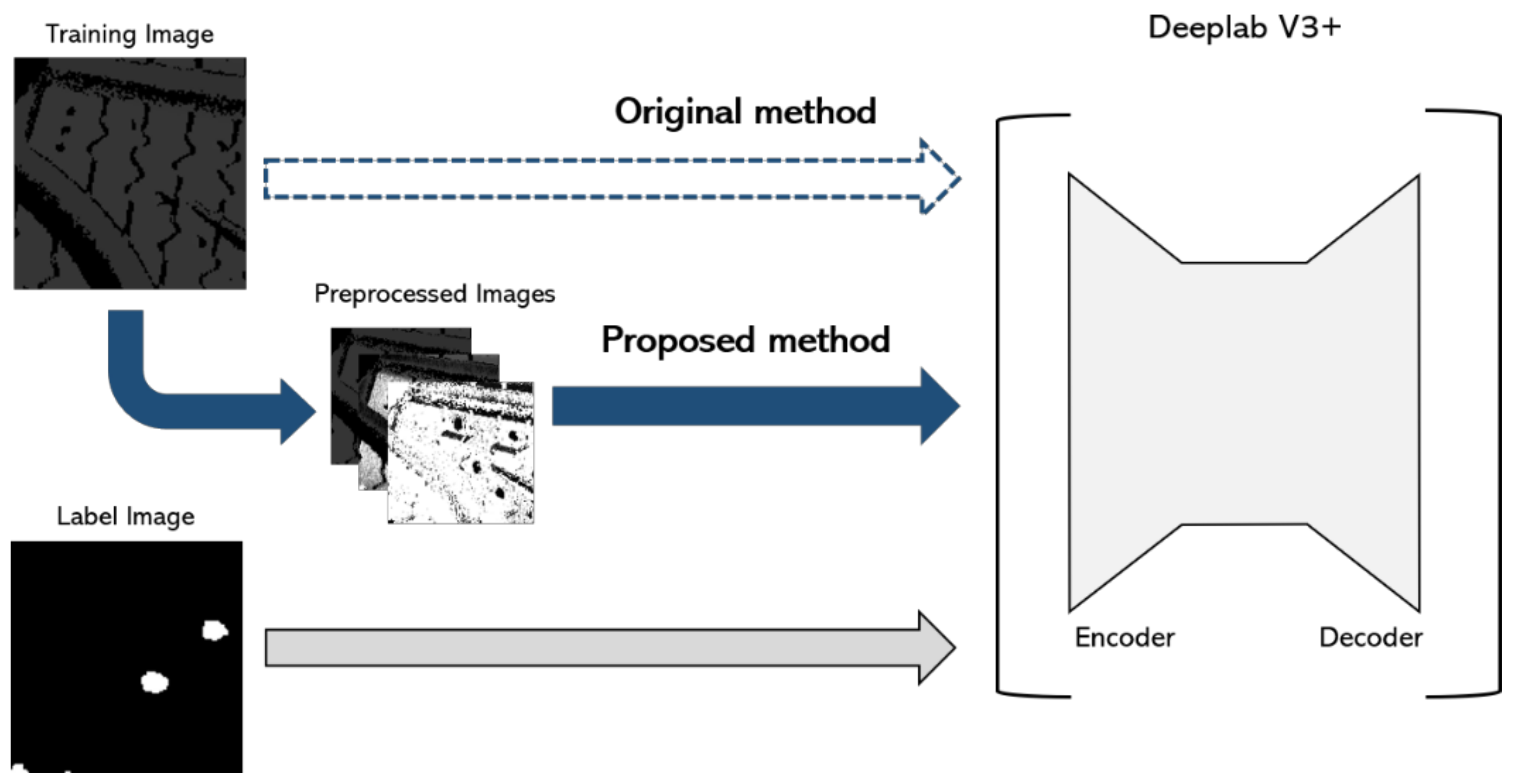
2. Materials and Methods

This section introduces the process and architecture of preprocessing depth image data for efficient tire defect detection and training. For tire error detection, a depth image having tire height information is acquired, using a 3D camera, and this image is used to detect defects in the tire.
The tire depth image contains depth information that best describes the error that may occur in the tire. However, (1) the height value is concentrated in a narrow section, and (2) with the same tire error, the shape is often different. For these two reasons, there is a limit to the error detection accuracy when the deep learning model trains using only pure depth images. Although this paper aims to classify the area of vent spew error, it must have the robustness to classify additional errors in the future. In other words, it should not damage the original data, and show maximum classification performance.
Therefore, this paper generates three images based on the original depth image: (1) the original image, (2) a histogram equalization depth image, and (3) a height information heatmap image. A heatmap is a graphical representation of data in which data values are represented as colors. These images are stacked into one three-channel image and used for deep learning network training. Histogram equalization data can compensate for the phenomenon that height data are concentrated in a narrow section, and heatmap data inform the degree of the anomaly of height values in depth images. By providing these additional data as training information, better results are obtained. Figure 1 compares deep learning, using original depth images and the learning method presented in this paper.

2.1. System Process

This paper uses the depth image containing 16-bit depth information. The vent spew error, which is the target of detection, mainly appears in the form of a protrusion from the tire’s surface. However, errors can be found at low height points in the depth image, such as tears and dents. Therefore, data preprocessing that is specialized for vent spew errors, such as filtering values above a certain height, is unsuitable for the training and detection of different errors, as it loses information on the lower height part.
This section introduces a depth image preprocessing process that efficiently trains and detects tire vent spews and prevents the loss of existing information. The image preprocessing process consists of 4 steps: (1) image input, (2) highlighted image creation, (3) image stacking, and (4) image training. Figure 2 shows the four-step process of preprocessing the depth image before training the tire error.
In this paper, we use the DeeplabV3+ model—one of the image segmentation models—to train and detect atypical errors. Figure 3 shows a schematic detailing the application of the four-step process to train the DeepLab model.

2.2. Step 1: Image Input

This step is the step of loading the image to train the tire depth image. We created tire depth images for training and labeled images that indicate errors in the training images to train the image segmentation model. In this paper, we defined a vent spew error, which is more than 2 mm from the tire surface among vents. Figure 4 shows the vents on the tire tread. Since it is difficult to judge an image expressed in depth with the naked eye, this is an example taken with an RGB camera. Figure 4 shows the tire tread taken with a general RGB camera to help understand the vent spew error. In Figure 4a, the vents are points protruding from the tire surface. The green circle in Figure 4a indicates one of the vents. Among these vents, a vent with a length of 2 mm or more is a vent spew error. Figure 4b shows the results of labeling vent spew errors in yellow. The green circle in Figure 4b indicates one of the vent spew errors.
To express the tire surface as a depth image, we used the following method. (1) First, a laser is fired on the tire tread surface that rotates with a constant angular velocity. (2) The fired laser is photographed with a 3D camera positioned at an angle of 30 degrees. (3) The captured image is converted into a depth image. Because the 3D camera captures the tire surface at an angle of 30 degrees, shadows may appear when photographing the vent spew error, which shows the shape protruding from the tire surface. Areas of unknown depth, such as shadow areas, have a value of 0. The depth image is mapped to an integer range (0 to 65,535), according to the degree of protrusion. Figure 5 shows the conversion of the surface of the tire into a depth image, using a laser.
We compared the actual tire with the depth image taken to label the vent spew error, and measured a vent greater than 2 mm. Since the depth image composed of 16-bit integers has an extensive range of values, it is difficult for the naked eye to distinguish between high and low points. Therefore, we performed labeling by comparing it with the depth image converted to 3D form and the actual location. Figure 6 shows a part of the photographed tire tread depth image labeled accordingly.

2.3. Step 2: Highlight Image Creation

In Step 2, creating a highlight image provides the classifier with additional information other than depth information. The tire depth image taken in this paper expresses height information as a 16-bit integer (0 to 65,535), but errors, such as vent spew, occurring in tires have a small height difference of about 0.1 mm. In addition, since the difference in the height change of the tire surface is not large, the data are concentrated in a certain section in the entire range. Such data concentration may cause difficulties in training, because height difference information is lost in the data normalization process before training, or the distance difference between pixels is very narrow. Therefore, in Step 2, additional image data based on the original data are created to reinforce this problem.

2.3.1. Histogram Equalization

In order to compensate for data loss that may occur in data normalization and the minimization of the height difference between pixels, an image obtained by performing histogram normalization on the present image is generated. Since there is almost no difference in height, except for areas where errors do not occur, the height data are concentrated in one section. In the process of normalizing the height values concentrated in a narrow range to a real number (between 0 and 1) for training, information on the height difference between pixels may be lost. In addition, in scanning the tire surface with a 3D camera, all values of the tire surface that were not measured due to shadows are filled with zeros, so the ratio of zero values in the depth image is high. We performed histogram smoothing, using the accumulated values of the image histograms.
Histogram smoothing is a method of rearranging contrast values to emphasize the contrast in grayscale images [55,56,57]. We measured the distribution of image brightness values through the histogram distribution of depth images. The histogram of an image can be obtained by calculating the frequency of the image pixel values. Algorithm 1 shows the process of histogram smoothing of the image, while Figure 7 compares the original image and the histogram smoothed image.
ALGORITHM 1: 16BIT IMAGE HISTOGRAM EQUALIZATION
Applsci 11 10376 i001

2.3.2. Histogram Heatmap

When looking at the defect detection process in the tire from an anomaly detection point of view, the height information of the defect location is more likely to have an exceptional value than elsewhere in the image. Thus, an image weighing the pixel value of the image is created and included in the training data. The pixel value weight is defined as the number of current pixel values for the entire image. Therefore, the weight value of the normal tire surface is higher than the weight value of the abnormal surface. This weighted image cannot be computed by convolution by an image filter. Therefore, the weighted image provides additional data, and the DeepLabV3+ network cannot infer that through the inside convolution layer. In addition, it helps to improve the training speed by expressing unusual parts of the tire surface with a low value during the training process. Figure 8 shows the weighted image calculated based on the input image. The normal tire surface is expressed brightly in this weighted image, while the abnormal or rare value is expressed darkly.

2.4. Step 3: Image Stacking

In Step 3, (1) the original image, (2) the histogram smoothed image, and (3) the weighted images are stacked to create a three-channel image. We normalized the data since the original image, the histogram smoothed image, and the weighted image all have different pixel values. Figure 9 shows a three-channel image created by stacking three images. Before stacking images, we changed the image data format to a 32-bit float type and normalized it to a range of (0 to 255). This operation minimizes data loss during deep learning model training.

2.5. Step 4: Image Training

DeepLab V3+ model training is performed based on images and labels with added information. The average size of the images taken with the actual 3D camera is vast, with a width of 10,000 px and a height of 1024 px, so the training is carried out through a separate process, as follows: (1) Crop the tire image into a square shape suitable for DeepLabV3+ training, and save it. (2) Load the saved image. (3) Preprocess through Steps 1–3. (4) Put the image and label into the DeepLabV3+ model to train it. When cropping and saving the tire image, the sliding window is moved and cut by half the crop size to compensate for the defective part being divided, and the overall shape is not trained. When the sliding window moves to the edge of the image, if the size of the tire image included is smaller than the window, it is stored with 0 paddings.

2.6. System Architecture

The tire fault detection system consists of a depth image scan and labeling that creates a depth image for training and actual tire inspection, and a tire fault inspection system that trains a deep learning model, and detects defects. Figure 10 shows the overall system architecture.

2.6.1. Depth Image Scan and Labeling

A 3D camera scans the finished tire to create a depth image. If it is not a training tire, it sends the image to the tire defect inspection system. When used as training data for the system, pixel-by-pixel labeling of erroneous and healthy pixels is performed.

2.6.2. Tire Fault Inspection System

The system trains tire defects and inspects defects, using the trained weights. When the tire inspection is completed, the detected defect area is visually communicated to the operator. If erroneous detection or non-detection error occurs, the operator re-labels relevant parts, and includes them in the training data.
  • Data loader
The data loader loads tire depth images for defect detection and training. If the load data are training, the label data paired with the training data are also loaded.
Data matching module: This module lists data for training and inspection and loads in order. When importing training data, it lists label data pairs that match the data. In addition, it separates the data into training data and validation data. When one epoch is finished during training, the training data set is randomly shuffled, and then loaded in order.
Data slice module: The tire depth image is a long horizontal rectangle and is very large. Therefore, a significant amount of GPU memory is required for training and detection. Thus, the imported tire data are cut and used for training and detection. Tire data are cut into a square shape. If the error region is located on the cut surface, it may not train the complete error form. Considering this, when slicing the image, we slide by 1/2 of the slice size. In this paper, data are sliced with a step of 64 px in a 128 px square shape. The excess area that may occur while cutting the data is solved by filling the remaining area with zeros.
Data stacking module: A three-channel image is created through the four processes proposed in this paper. Finally, we use this image for training and error detection.
  • Inspector
Deep learning network training is performed through preprocessed data. Tire defect inspection is performed based on the weights that are trained.
Model training module: If previously trained model weights exist, deep learning model training is performed based on those model weights. If there are no trained model weights, training is performed from the beginning.
Weight applying module: The training result weight is applied to the tire inspection module. One of two types of weights can be used: (1) the weight of the epoch with the highest validation accuracy during training, or (2) the weight of the last epoch considering further training.
Fault inspecting module: Defect areas are detected in the tire image based on the applied weights.
  • Visualizer
The visualizer visually shows the training process or actual tire error detection results.
Result visualizing module: When training, this module shows various training indicators, such as test, validation data-based loss, mean IoU, and validation results in real-time. In the case of tire error detection, the cut-out tire images are merged to show the area of the defect in the entire tire image.
Feedback module: As a result of detecting a tire defect, false detection or data requiring additional training may be generated. At this time, the corresponding data are additionally labeled, and later included in the training data.

3. Experimental Evaluation

This chapter describes (1) tire depth image training using a general method, and (2) tire depth image training through the preprocessing proposed in this paper. For accurate experiments, we use the same hyperparameters and datasets. For the quantitative evaluation of the investigation, the precision, recall, and f-score for each training result are compared. Additionally, we compare the training results for several sub-models that can be applied to the DeepLabV3+ model. Table 1 shows the device specifications used for model training in this paper.
A total of 18 types of tire images were used for model training. We cropped the whole tire image in an 8:2 ratio for training, then used 80% of the images for training, and the rest for validation. Each image was cropped in a square shape with a width of 128 px and a height of 128 px.
Since the proportion of vent spew errors in tire images is very small, most of the cropped images are images without vent spew errors. Since the imbalance in the normal data and bad data in the training data can lead to poor training results [58], we included only 5% of images with no vent spew error in the training and validation images. As a result, 5686 training data and 1425 validation data were generated. Figure 11 shows a sample image and labeling data used for training.
We trained all training data through 1000 iterations (1000 epochs). The initial value of the learning rate was 0.001. In this experiment, weight decay was set to 0.0001, and momentum to 0.9. Additionally, we applied a polynomial strategy, such as Equation (1) [59], to the training process. That caused the learning rate to gradually decrease, so that as the learning parameter approached the optimal value, the performance was stable.
p o l y = 1 c u r   i t e r t o t a l   i t e r p o w e r
Finally, the output stride of DeepLabV3+ was 8, and the convolution neural network inside the model was resnet-101. The batch size was set to 150. Data segmentation divides the classes into units of pixels. Since the number of pixels in the vent spew error in the training data set image is relatively small, the number of pixels per class is highly unbalanced. Therefore, in this experiment, in calculating the training loss using the cross-entropy function, weights for each class were applied to compensate for the imbalance. The pixels in the vent spew error region occupy about 5% of the total pixels in the training data, so a weight of 0.05 was applied to the normal class, and 0.95 to the vent spew class.

3.1. Evaluation Methods for the Segmentation

3.1.1. Precision, Recall, and F1-Score Analysis

Precision is the ratio of the number of positive pixels predicted correctly to all predictive positive pixels. Recall is the ratio of the number of correctly predicted positive pixels to the total of true positive pixels. Equations (2) and (3) define the precision and recall.
P r e c i s i o n = T P T P + F P
R e c a l l = T P T P + F N
where TP is true positive, which is a pixel that is predicted to be positive and is actually positive; FP is false positive, which is a pixel predicted to be positive, but is actually negative; FN is false negative, which is a pixel predicted to be negative but is actually positive.
The F1-score is a combination of precision and recall. Since precision and recall are in a trade-off relationship, they might have extreme values. Additionally, like the data used in this paper, when the imbalance between the number of normal classes and error classes is severe, it compensates for this. Equation (4) shows the F1-score.
F 1   score = 2   P r e c i s i o n R e c a l l P r e c i s i o n + R e c a l l

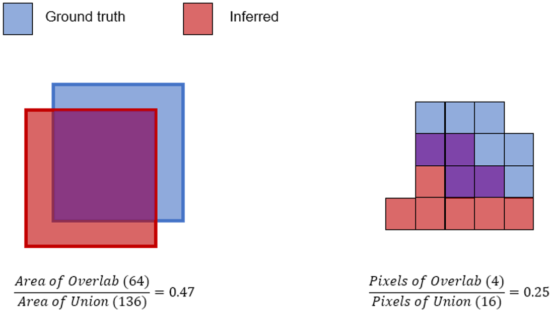
3.1.2. Intersection of Union (IoU)

IoU is the most popular evaluation method for object detection benchmarks. Many object detection methods in computer vision use a bounding box to indicate the interest object’s location. IoU is calculated using the bounding box of the ground truth and the bounding box inferred from the object detection method. Equation (5) shows the calculation for IoU.
IoU = Ground   truth   area   Inferred   area Ground   truth   area   Inferred   area
Object segmentation methods–based deep learning describes object location using pixel-wise, not bounding box. So, we calculate IoU using the pixel count but with the bounding box’s area. Figure 12 describes the comparison of two methods: the bounding box-based and pixel-based methods.

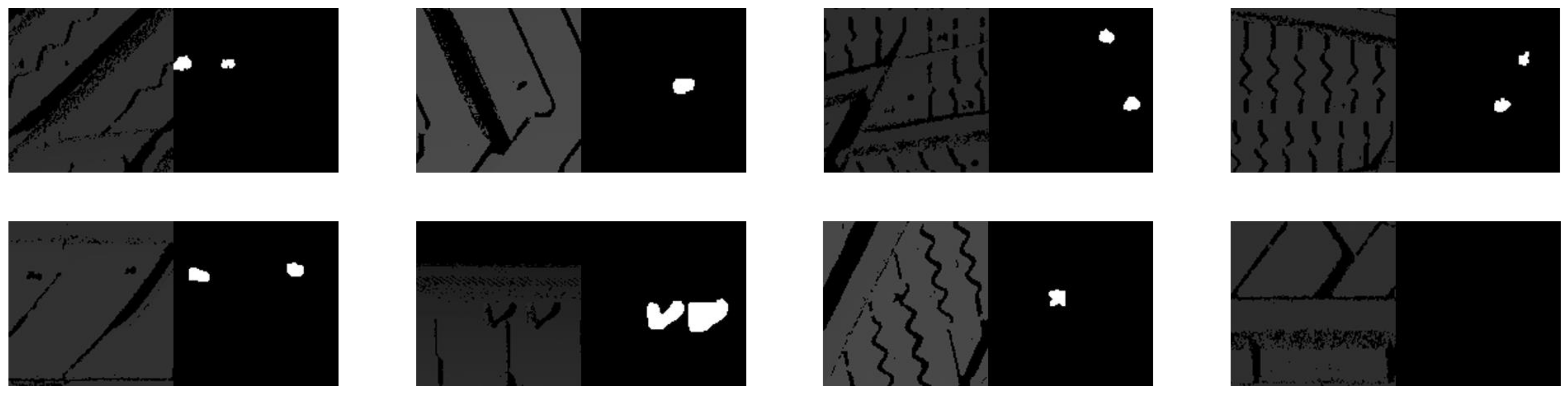
3.2. Training Results

We compare the mean IoU of the proposed method and the original method to evaluate. The original method uses the raw depth image data (one channel) for training without extending it to three channels though the proposed method. At the end of data training for one epoch, IoU is calculated from the validation data. We use the average value of the IoUs of this verification data as the accuracy index of the deep learning model.
For comparison, (1) original 1-channel depth image, and (2) 3-channel image with additional information were used as training data, based on the same model and hyperparameters. As a result of training, the proposed method showed a mean IoU improvement of about 7%, compared to the original method. Figure 13 compares the validation of the mean IoU of the original method and the proposed method. Defect areas were inferred from the test image based on the weights in the last epoch. Figure 14 shows the inference results.
We measured the average IoU data for the training set and the separate validation set with 1000 iterations of training. In Figure 13, it can be seen that the proposed method converges more stable than the original, and training proceeds. In the original method, the time point at which the mean IoU was stably maintained above 0.61 was 516 epochs, but in the case of the proposed method, the time was shortened by about 80% to 100 epochs.
In addition, various performance indicators were derived through various CNN networks (Mobilenet, Resnet-50, and Resnet-101) that can be applied inside the DeepLabV3+ model. As a result of the test, the precision/recall values in units of image pixels were derived, and the harmonic average of these values, the F1-score, was calculated.
When the model using Resnet-101 with the best performance was compared, the precision result of the proposed method was found to be lower than that of the existing method. However, it was deduced that the F1-score value, which is the harmonic average with recall, increased, resulting in reliable results, compared to the existing method. Table 2 shows the results of these indicators.

3.3. Discussion

The method proposed in this paper preserves the existing original data; at the same time, it generates additional data that cannot be extracted through the CNN network, and performs training based on the data, showing higher performance compared to the existing method. In addition, maintaining the original data without data preprocessing through filters, such as height threshold values, shows robustness to additional error training in the future.
The proposed method has improved precision, recall, and F1-score values, compared to the previous one, but it is not excellent given absolute value. The reasons for this are the (1) lack of data and (2) inclusion of human error.
It takes a long time to collect enough tire error data of the same kind for training. The methodology presented in this paper also has the purpose of compensating for the lack of data. However, as the number of data increases, the absolute precision and recall values will increase.
In the data labeling performed in this paper, a person directly measures the length of the vent spew error and labels the depth image data. Additionally, since the area of error data is determined by the person, it is inconsistent. For example, it is ambiguous whether only the pixels of the rubber hair where the error occurred is taken as the error area or the area around it. A more accurate error measurement and labeling method will improve the results.
Furthermore, in the training process, the training loss converges to 0 in both methods, but the validation loss diverges after a certain epoch. Figure 15 shows the training/validation loss in the training processes of the original and proposed methods.
This type of graph occurs because the error criteria and labeling for the vent spew error are ambiguous. The vent spew error is a vent protruding more than 2 mm from the tire surface, and the vents protruding from the tire surface are clustered around this 2 mm. Because differences in increments of 0.1 mm are difficult to recognize by the ordinary person and by the naked eye, data labels are ambiguous, unless vents larger than 2 mm are clearly identified. In addition, data according to the degree of inclination of the vent protrusion is not considered, so if it exceeds 2 mm but is attached to the tire surface, it can be recognized as a normal vent.
Therefore, in future research, for improving precision, recall, and training loss, we will study the classification method that considers the accurate measurement criteria of vent spew error and the protrusion angle of the vent.

4. Conclusions

This paper introduced and implemented the process of segmenting the vent spew error, a type of tire failure error, through the four steps of (1) image input, (2) highlight images creation, (3) image stacking, and (4) image training. Detecting a vent spew error in which rubber hairs protrude more than 2 mm from the tire tread is an inefficient task because it is necessary to measure the protrusion lengths for the number of rubber hairs existing in one tire. Therefore, in this paper, the vent spew error was easily and quickly detected by acquiring the height value of the tire surface with a 3D camera, and training a deep learning network with it during the tire inspection process. However, since the height values measured by the 3D camera were concentrated in a narrow range, the performance when training only the depth image of one channel was not good.
Therefore, in this paper, based on the existing data, it was easy to train for other errors in the future, so additional data of the (1) histogram equalization, and (2) histogram heatmap images were generated and included in the training data. In this proposed method, the original data were not lost.
The existing one channel depth image training results were compared with the results trained through the proposed process for experiments and evaluations. As a result of the experiment, both the mean IoU and the vent spew error detection rate increased by about 7–10%, respectively. The epoch was shortened by 80% during training, until the average IoU remained stable at 61%. However, there was limited accuracy to classify the atypical rubber hairs that protrude more than 2 mm from the tire surface based on the depth image with only a tiny difference in one-dimensional height information. This limitation is explained by a graph in which the training and validation losses do not converge but diverge. In addition, since the tire tread photographed with a 3D camera has a curved shape, it is necessary to correct the height of the center part and the edge part of the tire. To solve these limitations, we plan to research more accurate vent spew error measurement in the future: methods, standards, and depth image generation.
The introduction of artificial intelligence technology into the visual inspection stage, which can be the last stage of the manufacturing process, is expected to greatly increase productivity by eliminating inspection errors that arise because each operator has different skill levels and error evaluation standards.

Author Contributions

Conceptualization, D.K. and H.K.; methodology, D.K.; software, D.K. and H.K.; validation, S.K., W.L. and Y.B.; formal analysis, J.P.; investigation, D.K. and S.K.; resources, W.L.; data curation, D.K.; writing—original draft preparation, D.K.; writing—review and editing, S.K.; visualization, D.K.; supervision, J.P.; project administration, Y.B.; funding acquisition, Y.B. All authors have read and agreed to the published version of the manuscript.

Funding

This work was supported by the Ministry of Science and ICT (MSIT), Korea, through the Grand Information Technology Research Center Support Program supervised by the Institute for Information and communications Technology Planning and Evaluation (IITP) under Grant IITP-2020-0-101741.

Institutional Review Board Statement

Not applicable.

Informed Consent Statement

Not applicable.

Data Availability Statement

The data availability statements are listed as follows: the experiment results data used to support the findings of this study are partly available from the corresponding author upon request.

Conflicts of Interest

The authors declare that they have no conflict of interest.

References

  1. Uysal, M.P.; Mergen, A.E. Smart manufacturing in intelligent digital mesh: Integration of enterprise architecture and software product line engineering. J. Ind. Inf. Integr. 2021, 22, 100202. [Google Scholar] [CrossRef]
  2. Gao, G.; Zhou, D.; Tang, H.; Hu, X. An intelligent health diagnosis and maintenance decision-making approach in smart manufacturing. Reliab. Eng. Syst. Saf. 2021, 216, 107965. [Google Scholar] [CrossRef]
  3. Kang, H.S.; Lee, J.Y.; Choi, S.; Kim, H.; Park, J.H.; Son, J.Y.; Kim, B.H.; Do Noh, S. Smart manufacturing: Past research, present findings, and future directions. Int. J. Precis. Eng. Manuf. Green Technol. 2016, 3, 111–128. [Google Scholar] [CrossRef]
  4. Davis, J.; Edgar, T.; Porter, J.; Bernaden, J.; Sarli, M. Smart manufacturing, manufacturing intelligence and demand-dynamic performance. Comput. Chem. Eng. 2012, 47, 145–156. [Google Scholar] [CrossRef]
  5. Mittal, S.; Khan, M.A.; Romero, D.; Wuest, T. Smart manufacturing: Characteristics, technologies and enabling factors. Mech. Eng. Part B J. Eng. Manuf. 2019, 233, 1342–1361. [Google Scholar] [CrossRef]
  6. Li, Q.; Wang, L.; Shi, L.; Wang, C. A data based production planning method for multi-variety and small-batch production. In Proceedings of the 2nd International Conference on Big Data Analysis, Beijing, China, 1–12 March 2017; pp. 420–425. [Google Scholar]
  7. Wang, Y.; Ma, H.-S.; Yang, J.-H.; Wang, K.-S. Industry 4.0: A way from mass customization to mass personalization production. Adv. Manuf. 2017, 5, 311–320. [Google Scholar] [CrossRef]
  8. Wu, Z.-G.; Lin, C.-Y.; Chang, H.-W.; Lin, P.T. Inline inspection with an industrial robot (IIIR) for mass-customization production line. Sensors 2020, 20, 3008. [Google Scholar] [CrossRef]
  9. Robertson, I.D.; Yourdkhani, M.; Centellas, P.J.; Aw, J.E.; Ivanoff, D.G.; Goli, E.; Lloyd, E.M.; Dean, L.M.; Sottos, N.R.; Geubelle, P.H.; et al. Rapid energy-efficient manufacturing of polymers and composites via frontal polymerization. Nat. Cell Biol. 2018, 557, 223–227. [Google Scholar] [CrossRef]
  10. Schleinkofer, U.; Laufer, F.; Zimmermann, M.; Roth, D.; Bauernhansl, T. Resource-efficient manufacturing systems through lightweight construction by using a combined development approach. Procedia CIRP 2018, 72, 856–861. [Google Scholar] [CrossRef]
  11. Wu, B.; Hu, B.; Lin, H. Toward efficient manufacturing systems: A trust based human robot collaboration. In Proceedings of the 2017 American Control Conference, Seattle, WA, USA, 24–26 May 2017. [Google Scholar]
  12. Mourtzis, D. Simulation in the design and operation of manufacturing systems: State of the art and new trends. Int. J. Prod. Res. 2020, 58, 1927–1949. [Google Scholar] [CrossRef]
  13. Hu, H.; Wu, Q.; Zhang, Z.; Han, S. Effect of the manufacturer quality inspection policy on the supply chain decision-making and profits. Adv. Prod. Eng. Manag. 2019, 14, 472–482. [Google Scholar] [CrossRef]
  14. Lopes, R. Integrated model of quality inspection, preventive maintenance and buffer stock in an imperfect production system. Comput. Ind. Eng. 2018, 126, 650–656. [Google Scholar] [CrossRef]
  15. Iglesias, C.; Martínez, J.; Taboada, J. Automated vision system for quality inspection of slate slabs. Comput. Ind. 2018, 99, 119–129. [Google Scholar] [CrossRef]
  16. Chen, S.; Xiong, J.; Guo, W.; Bu, R.; Zheng, Z.; Chen, Y.; Yang, Z.; Lin, R. Colored rice quality inspection system using machine vision. J. Cereal Sci. 2019, 88, 87–95. [Google Scholar] [CrossRef]
  17. Lee, S.; Kim, J.; Lim, H.; Ahn, S.C. Surface reflectance estimation and segmentation from single depth image of ToF camera. Signal Process. Image Commun. 2016, 47, 452–462. [Google Scholar] [CrossRef]
  18. Frangez, V.; Salido-Monzú, D.; Wieser, A. Surface finish classification using depth camera data. Autom. Constr. 2021, 129, 103799. [Google Scholar] [CrossRef]
  19. Du Plessis, A.; Yadroitsava, I.; Yadroitsev, I. Effects of defects on mechanical properties in metal additive manufacturing: A review focusing on X-ray tomography insights. Mater. Des. 2020, 187, 108385. [Google Scholar] [CrossRef]
  20. Liu, W.; Chen, C.; Shuai, S.; Zhao, R.; Liu, L.; Wang, X.; Hu, T.; Xuan, W.; Li, C.; Yu, J.; et al. Study of pore defect and mechanical properties in selective laser melted Ti6Al4V alloy based on X-ray computed tomography. Mater. Sci. Eng. A 2020, 797, 139981. [Google Scholar] [CrossRef]
  21. Millon, C.; Vanhoye, A.; Obaton, A.-F.; Penot, J.-D. Development of laser ultrasonics inspection for online monitoring of additive manufacturing. Weld. World 2018, 62, 653–661. [Google Scholar] [CrossRef]
  22. Xiang, Y.; Zhang, C.; Guo, Q. A dictionary-based method for tire defect detection. In Proceedings of the 2014 IEEE International Conference on Information and Automation, Cluj-Napoca, Romania, 22–24 May 2014; pp. 519–523. [Google Scholar]
  23. Li, J.; Huang, Y.; Junfeng, L. Automatic inspection of tire geometry with machine vision. In Proceedings of the 2015 IEEE International Conference on Mechatronics and Automation, Beijing, China, 2–5 August 2015; pp. 1950–1954. [Google Scholar]
  24. Fachada, S.; Bonatto, D.; Schenkel, A.; Lafruit, G. Depth image based view synthesis with multiple reference views for virtual reality. In Proceedings of the 3DTV-Conference: The True Vision—Capture, Transmission and Display of 3D Video, Piscataway, NJ, USA, 3–5 June 2018; pp. 1–4. [Google Scholar]
  25. Han, T.; Nunes, V.X.; Souza, L.F.D.F.; Marques, A.G.; Silva, I.C.L.; Junior, M.A.A.F.; Sun, J.; Filho, P.P.R. Internet of medical things—Based on deep learning techniques for segmentation of lung and stroke regions in CT scans. IEEE Access 2020, 8, 71117–71135. [Google Scholar] [CrossRef]
  26. Du, Z.; Hu, Y.; Buttar, N.A.; Mahmood, A. X-ray computed tomography for quality inspection of agricultural products: A review. Food Sci. Nutr. 2019, 7, 3146–3160. [Google Scholar] [CrossRef]
  27. Zhang, G.; Jiang, S.; Yang, Z.; Gong, L.; Ma, X.; Zhou, Z.; Bao, C.; Liu, Q. Automatic nodule detection for lung cancer in CT images: A review. Comput. Biol. Med. 2018, 103, 287–300. [Google Scholar] [CrossRef] [PubMed]
  28. Zhang, R.; Zhuo, L.; Zhang, H.; Zhang, Y.; Kim, J.; Yin, H.; Zhao, P.; Wang, Z. Vestibule segmentation from CT images with integration of multiple deep feature fusion strategies. Comput. Med. Imaging Graph. 2021, 89, 101872. [Google Scholar] [CrossRef] [PubMed]
  29. Gudsoorkar, U.; Bindu, R. Fatigue crack growth characterization of re-treaded tire rubber. Mater. Today Proc. 2021, 43, 2303–2310. [Google Scholar] [CrossRef]
  30. Liu, H.; Lei, D.; Zhu, Q.; Sui, H.; Zhang, H.; Wang, Z. Single-image depth estimation by refined segmentation and consistency reconstruction. Signal Process. Image Commun. 2021, 90, 116048. [Google Scholar] [CrossRef]
  31. Turkoglu, M. COVID-19 detection system using chest CT images and multiple kernels-extreme learning machine based on deep neural network. IRBM 2021, 42, 207–214. [Google Scholar] [CrossRef] [PubMed]
  32. Grundy, L.; Ghimire, C.; Snow, V. Characterisation of soil micro-topography using a depth camera. MethodsX 2020, 7, 101144. [Google Scholar] [CrossRef] [PubMed]
  33. Wang, X.-B.; Li, A.-J.; Ci, Q.-P.; Shi, M.; Jing, T.-L.; Zhao, W.-Z. The study on tire tread depth measurement method based on machine vision. Adv. Mech. Eng. 2019, 11, 1–12. [Google Scholar] [CrossRef]
  34. Zheng, Z.; Zhang, S.; Yu, B.; Li, Q.; Zhang, Y. Defect inspection in tire radiographic image using concise semantic segmentation. IEEE Access 2020, 8, 112674–112687. [Google Scholar] [CrossRef]
  35. Zhang, Y.; Cui, X.; Liu, Y.; Yu, B. Tire defects classification using convolution architecture for fast feature embedding. Int. J. Comput. Intell. Syst. 2018, 11, 1056–1066. [Google Scholar] [CrossRef] [Green Version]
  36. Noh, H.; Seunghoon, H.; Bohyung, H. Learning deconvolution network for semantic segmentation. In Proceedings of the IEEE International Conference on Computer Vision, Las Condes, Chile, 11–18 December 2015; pp. 1520–1528. [Google Scholar]
  37. Ban, K.D.; Kim, J.H.; Yoon, H.S. Gender Classification of Low-Resolution Facial Image Based on Pixel Classifier Boosting. ETRI J. 2016, 38, 347–355. [Google Scholar] [CrossRef]
  38. Chen, L.C.; Papandreou, G.; Kokkinos, I.; Murphy, K.; Yuille, A.L. Deeplab: Semantic image segmentation with deep convolutional nets, atrous convolution, and fully connected crfs. IEEE Trans. Pattern Anal. Mach. Intell. 2017, 40, 834–848. [Google Scholar] [CrossRef]
  39. Yin, P.; Yuan, R.; Cheng, Y.; Wu, Q. Deep guidance network for biomedical image segmentation. IEEE Access 2020, 8, 116106–116116. [Google Scholar] [CrossRef]
  40. Wang, G.; Li, W.; Zuluaga, M.A.; Pratt, R.; Patel, P.A.; Aertsen, M.; Doel, T.; David, A.L.; Deprest, J.; Ourselin, S.; et al. Interactive medical image segmentation using deep learning with image-specific fine tuning. IEEE Trans. Med. Imaging 2018, 37, 1562–1573. [Google Scholar] [CrossRef]
  41. Chen, L.C.; Papandreou, G.; Schroff, F.; Adam, H. Rethinking atrous convolution for semantic image segmentation. arXiv 2017, arXiv:1706.05587. [Google Scholar]
  42. Chen, L.-C.; Zhu, Y.; Papandreou, G.; Schroff, F.; Adam, H. Encoder-decoder with atrous separable convolution for semantic image segmentation. In Advances in Autonomous Robotics; Springer: Berlin, Germany, 2018; pp. 833–851. [Google Scholar]
  43. Pang, G.; Shen, C.; Cao, L.; Hengel, A.V.D. Deep learning for anomaly detection. ACM Comput. Surv. 2021, 54, 1–38. [Google Scholar] [CrossRef]
  44. Al-Amri, R.; Murugesan, R.; Man, M.; Abdulateef, A.; Al-Sharafi, M.; Alkahtani, A. A review of machine learning and deep learning techniques for anomaly detection in IoT data. Appl. Sci. 2021, 11, 5320. [Google Scholar] [CrossRef]
  45. Sultani, W.; Chen, C.; Shah, M. Real-world anomaly detection in surveillance videos. In Proceedings of the 2018 IEEE/CVF Conference on Computer Vision and Pattern Recognition, Salt Lake, UT, USA, 18–23 June 2018; pp. 6479–6488. [Google Scholar]
  46. Wen, L.; Weixin, L.; Dongze, L.; Shenghua, G. Future frame prediction for anomaly detection—A new Baseline. In Proceedings of the 2018 IEEE/CVF Conference on Computer Vision and Pattern Recognition, Salt Lake, UT, USA, 18–23 June 2018. [Google Scholar]
  47. Lindemann, B.; Fesenmayr, F.; Jazdi, N.; Weyrich, M. Anomaly detection in discrete manufacturing using self-learning approaches. Procedia CIRP 2019, 79, 313–318. [Google Scholar] [CrossRef]
  48. He, Z.; Yuexiang, L.; Nanjun, H.; Kai, M.; Leyuan, F.; Huiqi, L.; Yefeng, Z. Anomaly detection for medical images using self-supervised and translation-consistent features. IEEE Trans. Med. Imaging 2021. [Google Scholar]
  49. Himeur, Y.; Ghanem, K.; Alsalemi, A.; Bensaali, F.; Amira, A. Artificial intelligence based anomaly detection of energy consumption in buildings: A review, current trends and new perspectives. Appl. Energy 2021, 287, 116601. [Google Scholar] [CrossRef]
  50. Pustokhina, I.V.; Pustokhin, D.A.; Vaiyapuri, T.; Gupta, D.; Kumar, S.; Shankar, K. An automated deep learning based anomaly detection in pedestrian walkways for vulnerable road users safety. Saf. Sci. 2021, 142, 105356. [Google Scholar] [CrossRef]
  51. Du, M.; Li, F.; Zheng, G.; Srikumar, V. Deeplog: Anomaly detection and diagnosis from system logs through deep learning. In Proceedings of the ACM SIGSAC Conference on Computer and Communications Security, Dallas, TX, USA, 3 November 2017; pp. 1285–1298. [Google Scholar]
  52. Lee, S.; Kwak, M.; Tsui, K.-L.; Kim, S.B. Process monitoring using variational autoencoder for high-dimensional nonlinear processes. Eng. Appl. Artif. Intell. 2019, 83, 13–27. [Google Scholar] [CrossRef]
  53. Mei, S.; Wang, Y.; Wen, G. Automatic fabric defect detection with a multi-scale convolutional denoising autoencoder network model. Sensors 2018, 18, 1064. [Google Scholar] [CrossRef] [PubMed] [Green Version]
  54. Aguilar, J.J.C.; Carrillo, J.A.C.; Fernández, A.J.G.; Pozo, S.P. Optimization of an optical test bench for tire properties measurement and tread defects characterization. Sensors 2017, 17, 707. [Google Scholar] [CrossRef] [PubMed] [Green Version]
  55. Kansal, S.; Purwar, S.; Tripathi, R.K. Image contrast enhancement using unsharp masking and histogram equalization. Multimed. Tools Appl. 2018, 77, 26919–26938. [Google Scholar] [CrossRef]
  56. Khan, M.F.; Khan, E.; Abbasi, Z. Segment dependent dynamic multi-histogram equalization for image contrast enhancement. Digit. Signal Process. 2014, 25, 198–223. [Google Scholar] [CrossRef]
  57. Wang, C.; Ye, Z. Brightness preserving histogram equalization with maximum entropy: A variational perspective. IEEE Trans. Consum. Electron. 2005, 51, 1326–1334. [Google Scholar] [CrossRef]
  58. He, H.; Garcia, E.A. Learning from imbalanced data. IEEE Trans. Knowl. Data Eng. 2009, 21, 1263–1284. [Google Scholar] [CrossRef]
  59. Rong, G.; Sham, M.K.; Rahul, K.; Praneeth, N. The step decay schedule: A near optimal, geometrically decaying learning rate procedure for least squares. arXiv 2019, arXiv:1904.12838. [Google Scholar]
Figure 1. Comparison of the existing training method and the proposed method.
Applsci 11 10376 g001
Figure 2. System process.
Applsci 11 10376 g002
Figure 3. Proposed image preprocessing step.
Applsci 11 10376 g003
Figure 4. Tire tread image was taken with an RGB camera: (a) original image; (b) overlapped image with vent spew error label.
Applsci 11 10376 g004
Figure 5. Tire depth image capture using a laser and 3D camera.
Applsci 11 10376 g005
Figure 6. Tire tread image taken with a 3D camera: (a) original image; (b) label image in pixels, and (c) depth image expressed in 3D.
Applsci 11 10376 g006
Figure 7. Comparison of the original image and the histogram equalized image: (a) original depth image (left), and its histogram (right); (b) histogram equalized depth image (left) and its histogram (right).
Applsci 11 10376 g007
Figure 8. Comparison of the original image and weighted image: (a) original image labeled with vent spew error; (b) weighted image based on the original image.
Applsci 11 10376 g008
Figure 9. Stacked image.
Applsci 11 10376 g009
Figure 10. The tire fault inspection system.
Applsci 11 10376 g010
Figure 11. Sample image data were used to train the model. In each image, the image on the left is the tire depth image (.tif), and the image on the right is the image marked vent spew error.
Applsci 11 10376 g011
Figure 12. Example of calculating intersection of union; the traditional object detection methods calculate IoU through the bounding box area of the detection object (left), but the segmentation methods perform pixel-wise calculations (right).
Applsci 11 10376 g012
Figure 13. Comparison of the mean IoU (validation set) per epoch between the original and the proposed methods.
Applsci 11 10376 g013
Figure 14. Trained network–based test results; the left side of each image is the ground truth, while the right side is the inference result.
Applsci 11 10376 g014
Figure 15. Training/validation loss for the (a) original and the (b) proposed method training.
Applsci 11 10376 g015
Table 1. Specs of the training machine.
Title 1Title 2
CPUIntel Core i9-10980XE
GPUNVIDIA GeForce RTX 3090, 24 GB Memory
MemoryDDR4, 128 GB
FrameworkPyTorch 1.8.0, CUDA 11.1, CUDNN 11.2
Table 2. Original/proposed training results for various underlying networks.
OriginalProposed
MobilenetResnet-50Resnet-101MobilenetResnet-50Resnet-101
Mean IoU0.60660.63620.62300.62890.66700.6791
Class IoU
(Vent spew error)
0.21920.27730.26710.26240.33830.3621
Precision0.37690.42350.59670.36640.48170.5010
Recall0.34370.44780.32600.48010.53190.5662
F1-Score0.35950.43420.42170.41570.50550.5316
Publisher’s Note: MDPI stays neutral with regard to jurisdictional claims in published maps and institutional affiliations.

