
Hierarchical Concept Learning by Fuzzy Semantic Cells


1
College of Computer Science, Zhejiang University, Hangzhou 310007, China
2
College of Industrial Design, Hubei University of Technology, Wuhan 430068, China
*
Author to whom correspondence should be addressed.
Appl. Sci. 2021, 11(22), 10723; https://0-doi-org.brum.beds.ac.uk/10.3390/app112210723
Submission received: 7 September 2021
/
Revised: 3 November 2021
/
Accepted: 10 November 2021
/
Published: 13 November 2021
(This article belongs to the Topic Methods for Data Labelling for Intelligent Systems)
Abstract
:Concept modeling and learning have been important research topics in artificial intelligence and knowledge discovery. This paper studies a hierarchical concept learning method that requires a small amount of data to achieve competitive performances. The method starts from a set of fuzzy prototypes called Fuzzy Semantic Cells (FSCs). As a result of FSC parameter optimization, it creates a hierarchical structure of data–prototype–concept. Experiments are conducted to demonstrate the effectiveness of our approach in a classification problem. In particular, when faced with limited training data, our proposed method is comparable with traditional techniques in terms of robustness and generalization ability.
1. Introduction
This work is mainly concerned with concept learning. Concept learning categorizes the process to partition samples into classes for the purpose of generalization, discrimination, and inference [1]. Concepts are the basis of most cognitive processes such as inference, learning, and reasoning [2,3,4]. Concept modeling is fundamental in the fields of cognitive science and artificial intelligence. The learning and modeling of fuzzy concepts, in particular, has been a hot topic in these two fields. One prominent work on the cognitive representations of concepts in natural language is the prototype theory [5,6]. Many classic machine learning algorithms are related to the prototype theory, such as K-means algorithm, KNN algorithm and so on. The modeling of concept vagueness in artificial intelligence has been dominated by ideas from fuzzy set theory as originally proposed by Zadeh [7,8]. Then Goodman and Nguyen provided a solid framework foundation for fuzzy conceptual representations [9]. Lawry and Tang introduced an approach to uncertainty modeling for vague concepts by combining the prototype theory and the random set theory [10,11]. In the following in-depth studies, they developed a semantic representation of modeling uncertain concepts called Information Cell [12,13,14]. Tang and Xiao [15] also adopt Fuzzy Semantic Cell (FSC) to name this model. Based on FSC, Tang and Xiao provided an efficient way for unsupervised concept learning [15].
Our motivation is to model concepts underlying data and to represent concepts as partitions of samples for further classification. Our work builds on the model given in [15] and is inspired by the set partition method based on conditional entropy described in [16]. The model called fuzzy semantic cell (FSC) comprises a prototype P, a distance function d, and a probability density function of granularity. This structure is considered as the smallest unit of vague concepts and the building brick of concept representation. In Tang and Xiao’s study, they proposed three principles for developing reasonable FSC: Maximum coverage, maximum specificity, and maximum fuzzy entropy. In this paper, we focus on solving supervised concept learning problems, particularly those with sparse data. We learn from Śmieja and Geiger [16] that the consistency of set segmentation can be measured using conditional entropy. This viewpoint has greatly impacted our understanding of fuzzy semantic cell optimization. We combine the above two approaches from a supervisory point of view to obtain a simplified way to build the FSC by replacing three principles with the conditional entropy minimization principle with the help of the Adam algorithm [17]. The Adam algorithm is an efficient method for solving unconstrained nonlinear optimization problems, and it has been widely used in the optimization of neural networks in recent years. Moreover, we also propose a hierarchical concept learning structure for modeling and learning abstract concepts to which the sample pertains. Our method’s direct applicability is to solve the classification task in the case of a few training samples (only 10% samples as the training set). In our experiments, our method is not only competitive on the classification accuracy but also has robustness and generalization capabilities. As for conventional methods, we choose the NaiveBayes algorithm [18], k-nearest neighbor (KNN) [19], Decision Tree (DT) [20], Support Vector Machine (SVM) [21], AdaBoost [22] and neural network algorithm to apply control experiments.
The remainder of this paper is organized as follows. In Section 2, we revisit the ideas of [15], which presents a cognitive structure of vague concepts named Fuzzy Semantic Cell (FSC). In Section 3, we present a detailed introduction to our proposed supervised hierarchical concept learning method based on FSC. Section 4 reports and analyzes various experimental results to demonstrate the effectiveness of our proposed method. Conclusions are presented in Section 5. Our source code in PyTorch [23] is publicly available on github.com/Ming0405/HCL_.
2. Fuzzy Semantic Cell
Tang and Lawry [10,11] introduced a novel cognitive structure to model the vague concept having the form “about P”, “similar to P” or “close to P”. In this paper, we continue the definition in Tang and Xiao’s work [15] named Fuzzy Semantic Cell.
Definition 1.
A fuzzy semantic cell for a vague concept on the domain Ω is a triple representation where is the prototype of , d is the distance metric which measures the neighborhood size of , and is the probability density function of the neighborhood size of the vague concept .
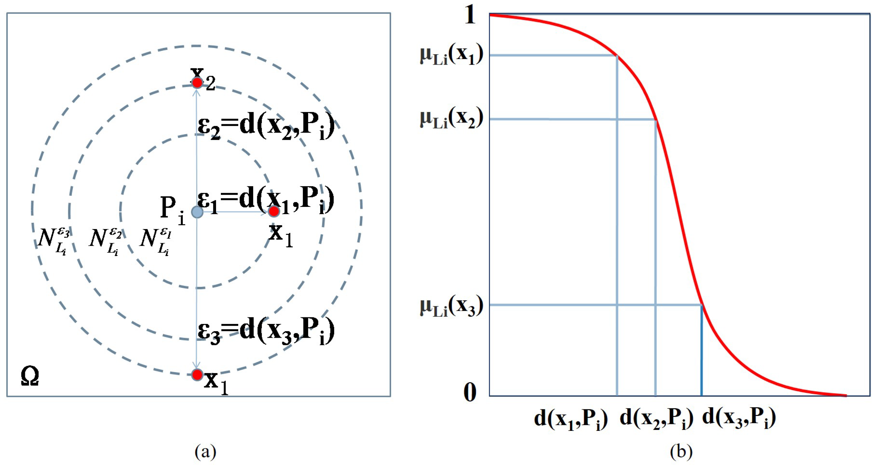
In other words, a fuzzy semantic cell for a vague concept is made up of a semantic cell nucleus represented by the prototype and a semantic cell membrane represented by an uncertain boundary of using d and . Hence, the fuzzy semantic cell is assumed to be the smallest semantic unit of vague concepts. Figure 1a shows a fuzzy semantic cell in two-dimensional space as an illustrative example.
Definition 2.
On the domain Ω, for any fuzzy semantic cell , and neighborhood size , the ϵ-neighborhood of is defined as follows:
According to Definition 2, the -neighborhood includes all the elements whose distance to the prototype is less than the given neighborhood size of , as shown in Figure 1a. Since is a random variable with the probability density function , can be considered as a random set neighborhood of . Therefore, for any , the degree of x belonging to the fuzzy semantic cell should be equal to the probability that the -neighborhood of is a set containing x, denoted by . Then, the neighborhood function of can be defined as follows.
Definition 3.
On the domain Ω, for any fuzzy semantic cell , and , the neighborhood function of is defined as follows:
We note that and is a decreasing function of the distance . In particular, when , ; when , . Thus can be the belief of a sample x being a neighbor of the the fuzzy semantic cell . Figure 1b shows an example of the neighborhood function of . Since is a decreasing function of the distance , an exponential form of is defined in [24] as follows:
where is the parameter of the probability density function , and it is related to the extent of the distribution. According to (2), the probability density function can be readily derived as follows:
Moreover, we use the following semimetric for d in this paper: . A semimetric on is a function that satisfies iff. and for .
3. Method
This section suggests a method for obtaining a hierarchical structure from data concerning the concept using the appropriate fuzzy semantic cells. First, a theoretical analysis of the proposed method is provided to demonstrate the rationality of this hierarchical structure. Then we explain The classification decision method based on the hierarchical structure. Finally, we present the principles of learning fuzzy semantic cell of a hierarchical structure, followed by the developed algorithm.
3.1. Hierarchical Structure of Concept Leaning
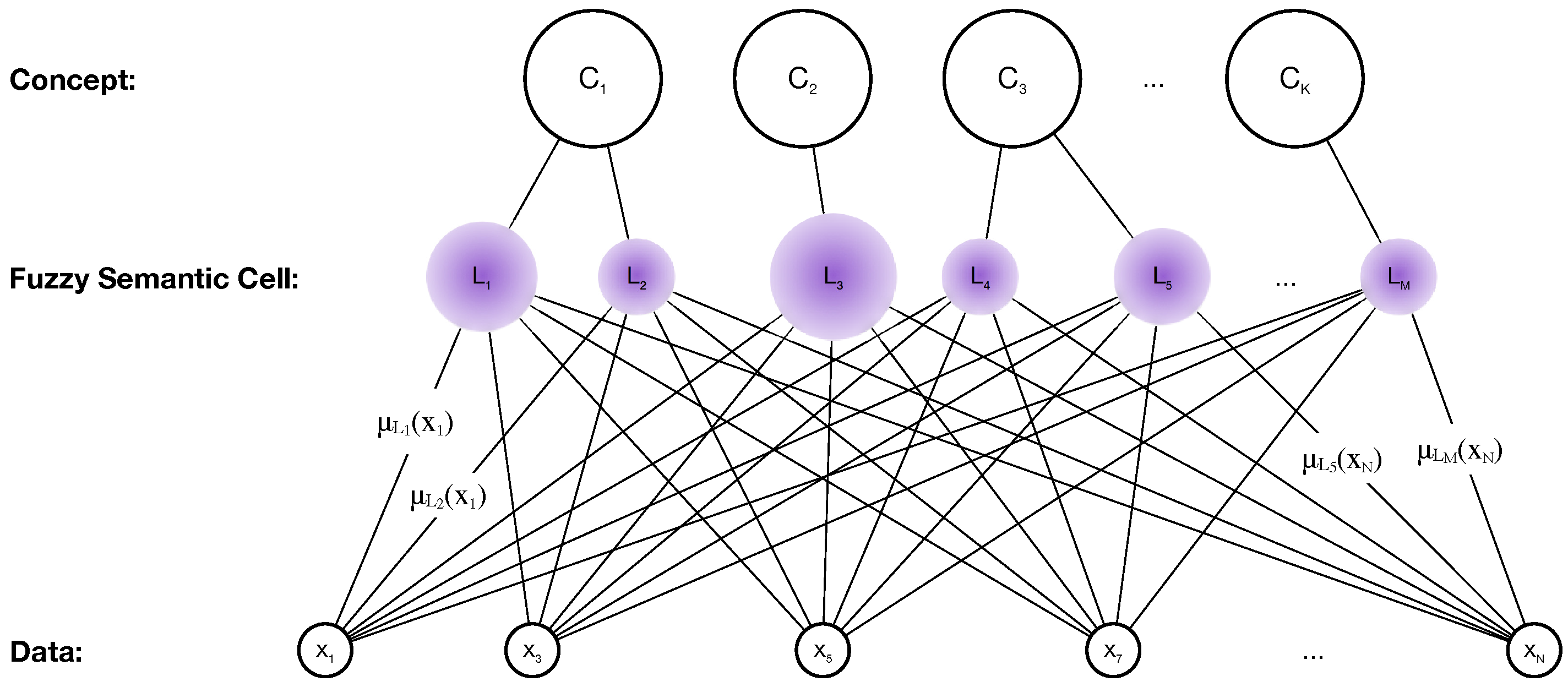
When people describe an abstract concept corresponding to a specific object, they may use one or more familiar prototypes in the explanation. These prototypes are highly relevant, and the boundaries between them are somewhat vague. Within a certain range, each prototype can explain the meaning of the object. Then, starting with these prototypes, we can achieve a higher level of abstraction to determine the concept’s meaning. We may only need one prototype for relatively clear and simple data; however, some more ambiguous and broad concepts may necessitate multiple prototypes to cover all interpretable ranges adequately. Considering account the ambiguous nature of abstract concepts, we develop a hierarchical concept learning model based on the fuzzy semantic cell. As shown in Figure 2, the hierarchical structure is composed of three layers. The bottom is the data layer, and the middle is the fuzzy semantic cell layer, the top is the conceptual layer. The membership degrees characterize the relationship between the samples in the data layer and the fuzzy semantic cells in the middle layer. In particular, indicates how well the semantic cell can interpret the sample x. Conversely, each fuzzy semantic cell can explain a range of different radii, covering a different number of samples in the data layer. Each concept is partitioned at the concept level by one or more FSCs. Because of the uncertainty and overlap of the boundaries between FSCs, this partition is ambiguous.
Formally, suppose we have a dataset with category information. This category information is a series of the abstract concepts. The can be partitioned into K subsets by category information:
where K is the number of categories, and we mark this partition way as S. In other words, is a subset of , and all of the elements x in belong to the same category.
At the same time, assume that can also be partitioned into , where is a fuzzy semantic cell with a prototype , a density function defined on , and a distance metric d on . Then, we will obtain the appropriate fuzzy semantic cell partition using the method described in Section 3.3.
3.2. Decision Rule of Classification
Based on the above discussion, we have got the hierarchical structure from known data to the concept. For a new sample x, the method to identify the abstract concept it belongs to is as follows:
- for new data , compute for all fuzzy semantic cells
- take the corresponding of maximum
- choose the concept that the belongs to as the abstract concept of x
3.3. Optimization of Fuzzy Semantic Cells
In this section, we will introduce the principles of learning FSCs. The proper partition means this partition makes the concepts of elements belonging to each are as consistent as possible. That is to say, the concept purity of elements covered by every is as high as possible.
To this end, for each concept (category), we compute the sum of the membership of all the elements under that concept to every fuzzy semantic cell marked . In fact, approximates the average number of samples covered by in :
Then we normalize all ’s for every to estimate the probability that samples covered by in :
As a result, the relative entropy of every is defined as:
We minimize to get the prior distribution for every fuzzy semantic cell.
As mentioned above, our goal is to get the which maximizes the concept purity. In other words, we need to find a partition of fuzzy semantic cells that is highly consistent with the concept partition. Our solution is inspired by the work [16]. In [16], the authors give the following definition of consistency of dataset segmentation:
Definition 4.
Let X be a finite dataset and let be the set of labeled data points that is partitioned into . A partition of X is consistent with Z, if for every there exists at most one such that .
Based on this, they proved that conditional entropy can be used to measure the consistency of dataset segmentation:
The smaller the conditional entropy is, the higher the consistency is. Inspired by this idea, we give the following definition of partition consistency of and S:
Definition 5.
Let be a finite dataset and is partitioned into . A partition of Ω is consistent with S, if for every there exists at most one such that .
Then we introduce the conditional entropy to our objective function to ensure is consistent with S. The conditional entropy in our scenario is defined as:
By minimizing the conditional entropy, we update the fuzzy semantic cells. The updating rule allows having the highest possible purity. At the same time, the parameter M controls the fine degree of FSCs. A proper number of M ensures that the fuzzy semantic cells are neither too rough nor too fine. is too fine means . In this case, too many FSCs correspond to the same category, although each has high internal purity, and each fuzzy semantic cell covers a very small radius. This will cause great redundancy. Especially in extreme circumstances, the partition will be perfect when is separated into a small portion which only contains one element, that is to say, M is equal to the number of items x. Because there are too many fuzzy semantic cells at this time, the computational complexity is high. Therefore, according to the premise of high purity, the FSCs in the same category, the better. As a result, we should include the constraint that M be as small as possible while be as pure as possible.
Finally, the learning problem of the hierarchical structure becomes an optimization problem of the objective function. Due to the difficulty in calculating the closed-form solution of this optimization problem, we use the iterative method instead. To obtain the optimal fuzzy semantic cell, we apply to Adam method [17], which is an efficient method to solve the unconstrained nonlinear optimization problems to minimize the objective function Equation (4). Existing works also use gradient descent [24], evolutionary optimization [26] or particle swarm optimization [27] to optimize the models. We believe numerical methods are more stable in optimization and Adam can avoid saddle points compared with gradient descent. The procedure of the hierarchical concept learning with fuzzy semantic cells is summarized in Algorithm 1.
| Algorithm 1 Hierarchical Concept Learning by Fuzzy Semantic Cells |
| Require: Training set of K categories with concept information where |
| Ensure: Fuzzy semantic cell |
| 1: function ()
: The dataset with concept information M: The numbers of fuzzy semantic cells |
| 2: Begin |
| 3: Partition: |
| 4: Initialize: |
| 5: for each data do |
| 6: Compute: |
| 7: Compute: |
| 8: end for |
| 9: Compute: minimize the following by Adam:
|
| 10: return |
| 11:end function |
The main runtime in our training is the computation of Equation (4), namely the conditional entropy. The computation complexity of Equation (4) is . This scales linearly with n, the number of samples. Empirically the computation only takes less than a second on a CPU of Intel Xeon 4116 in Ubuntu 16.04. Prototypes and are the parameters of our fuzzy semantic cells to optimize, and the only hyper-parameter having an influence is the number of prototypes. We will discuss it in Section 4.3.
In summary, we describe the learning method to build the hierarchical structure from the data to the concepts. Based on this structure, given a new sample x, we also introduce the decision-making approach to infer its abstract concept.
3.4. Discussion
In this part we discuss the similarity and differences between our proposed method and related supervised learning methods. The discussion is from four aspects: Prototype classification, hard/soft margin, limited samples and unsupervised learning.
Prototype classification. Prototype classification has been a thriving area in artificial intelligence. Mean-of-class prototype classification is a typical method to learn prototypes based on which classification is done [28]. There are three kinds of mean-of-class prototype classification methods. Non-margin classifiers, such as linear discriminant analysis (LDA) [29,30], form non-overlapping areas to represent concepts. Such methods use a similar strategy as our method to construct concepts. Other advanced works [31,32] introduce deep models to extract features for learning prototypes. However, one concept may have multiple prototypes and a non-margin classifier assumes only one prototype, while our method assumes multiple prototypes intrinsically.
Hard/soft margin. Hard margin classifiers include Support Vector Machine [21] and similar methods. They assume a hard hyper-plane or hyper-sphere to separate concepts. Such assumption does not consider the vagueness and uncertainty among samples, while our fuzzy semantic cells assume vagueness with an uncertain margin. Soft margin classifiers obtain prototypes by applying a regularized preprocessing and then classifying samples using hard margin classifiers [21]. This kind of methods also fail to consider multiple prototypes. Another typical soft margin classifier is mixture classification models [33,34]. The main idea is to fit Gaussian mixture models on samples in each class respectively and then to classify new samples with linear discriminant analysis. The fitting process is similar to our prototype learning procedure. However, our method further considers the exclusion among concepts with conditional entropy.
Limited samples. How to learn concepts with limited data is also a fundamental topic. As the number of samples is limited, prior knowledge [35], strong assumptions [36], appropriate augmentation [37,38] or transferred knowledge [39] is important. They can serve as an important inductive bias for out-of-distribution samples or regularize the model to avoid potential overfitting. The virtue that learning concepts from data can prevent adversarial attacks is also discussed [40]. Our method is based on the assumption of prototype theory [11] and the hierarchical structure of prototypes and concepts [24,25]. These two assumptions are from the perspective of how humans form concepts. Given the no-free lunch theorem, there is no universally applicable assumption. However, as our motivation is to model concepts, our assumptions of hierarchical prototypes are instructive.
Unsupervised learning. Prototypes and concepts learning has also been an important topic in unsupervised learning. With the assumption of density peaks [41], message propagation [42], mixture of distributions [43] or disjunctive combination [44], the underlying concepts can also be learned. A recent work [45] also extracts deep features for clustering. The motivation of the introduced unsupervised learning methods is also to learn concepts from samples, but the learning procedures are not supervised by labels. In summary, how to learn fuzzy concepts unsupervisedly with a reasonable assumption is an important topic in our future work.
4. Experiments
In this section, we conduct experimental studies of the proposed approach on five datasets.
4.1. Datasets
The description of each dataset is given as follows.
Synthetic dataset [15]: The synthetic two-dimensional dataset contains three classes. Each class follows the Gaussian distribution. The dataset contains 750 samples, and there are 250, 300 and 200 samples in each class, respectively.
Forest [46]: The Forest dataset is from UCI Machine Learning Repository. This dataset contains training and testing data from a remote sensing study which mapped different forest types based on their spectral characteristics at visible-to-near infrared wavelengths of four types (“s”-“Sugi” forest, “h”-“Hinoki” forest, “d”-“Mixed deciduous” forest, “o”-“Other” non-forest land). The original data contains 27 attributes, of which 1–9 are numerical spectral properties, 10–27 are non-numerical attributes. We only took the first nine columns of numerical properties for the experiment followed by merging the training set and the test set in the original data, a total of 523 samples as a 523 × 9 array.
Pendigits [47]: The dataset which is a digit database by collecting 250 samples from 44 writers stored in a 10,992 × 16 array. It is also from UCI Machine Learning Repository.
MNIST [48]: The MNIST database contains a total of 70,000 examples of handwritten digits of size 28 × 28 pixels. It is a subset of a larger set available from NIST. The digits have been size-normalized and centered in a fixed-size image.
MIT face [49]: This dataset from MIT contains synthetic face images of 10 subjects with 324 images per item. These synthetic images were rendered from 3D head models and stored as a 64 × 64 size figure. The final dataset is stored as an array of 3240 × 4096, containing ten different categories for a different subject.
Table 1 shows the summarized characteristics of five datasets involved in the experiment.
4.2. Initialization Method
The dataset needs to be preprocessed before starting the classification experiment. To ensure the rationality of the dataset segmentation, the data of each category is firstly extracted proportionally and then spliced together as the training set. Finally, we shuffle the samples in the training set, and the remaining data is regraded as the test set.
For the initialization of the parameter P, we try a variety of methods.
- The first one is to perform K-means on each type of training set and get the clustering centers as the initial prototypes.
- The second way is to get the clustering centers by K-means in the entire training set to get the initial prototypes.
- The third way is to select samples in each category as prototypes randomly.
- The last way is to take the average of each category of data as initialization.
Along with our paper, we assume the number of clusters in initialization is equal to the number of prototypes. The first three methods take a proportional number of prototypes M to the number of categories K. Notice that we define K is the number of categories, and K is not related to K-means in our scenario. The final method takes the mass centers of the samples from each class as the prototypes, and it assumes the number of prototypes equal to the number of categories. In the experimental section, we will compare these four initialization methods to investigate the effects of different prototype initialization methods.
For the parameter , as a parameter for controlling the bell-shaped distribution width, experiments show that the initialization of will affect the convergence speed and the classification result of the algorithm. Empirically we discovered that a better classification result can be obtained when the value of is one-third of the average distance between training set samples and the corresponding prototype. However, no additional theoretical support for this phenomenon has been discovered. We will leave it for future work.
4.3. Experimental Results
Table 2 shows the changes of classification accuracy under different training set scales. We repeat the experiment 100 times to obtain the mean and standard deviation of the classification results, considering the randomness of the dataset segmentation and differences in initializing parameters. In this experiment, we use the second initialization method of P. In particular, we use K-means to initialize one prototype in each class and then combine them together as the prototype initialization. As an initialization for , we take one-third of the average distances between the samples of each category and the prototypes. From the experimental results, we can see that our method is robust. Even in the case of a small amount of data (only 10%), we can get an acceptable classification result.
For the initialization of the prototype, we can limit the initialization method and the number of initial prototypes. In the following two experiments, 30% (3290 samples) of the Pendigits dataset were used as the training set and the rest as the test set (7702 samples).
Table 3 shows the difference in classification results for different numbers of prototypes. We initialize one to four prototypes in each category (a total of 10 categories) by K-means, so the number of prototypes ranges from 10 to 40 in the prototype initialization. We also set as one-third of the average distance that the samples of each category to the prototypes. We also repeated the experiment 10 times to obtain the mean and standard deviation of the classification results, taking into account the randomness of dataset segmentation and differences in initializing parameters. The experimental results are consistent with the above analysis. The classification effect will improve as the number of prototypes increases. As a result, as the number of prototypes grows, so the computational complexity also increases. At the same time, if there were too many prototypes, most fuzzy semantic cell will become too small and redundant. As a result, we must select the appropriate number of prototypes to strike a balance between computational efficiency and classification effect.
In the following experiment, we conducted a controlled trial in four ways as described in Section 4.2 to show the classification accuracy under different initialization methods of prototypes on Pendigits dataset as shown in Table 4. We used ten prototypes (), and the initialization method of is the same as before. The experiment is repeated six times. The experimental results show that the training accuracy decays slightly since more samples are difficult to fit. However, the testing accuracy increases substantially as the model learns more about the training distribution. Despite the objective function being a non-convex problem, the classification effect is nearly stable across the different prototype initialization methods. When prototypes are initialized by category, the results are consistent after repeated experiments, and the standard deviation is low. When the prototypes are initialized with a global method, the overall classification accuracy is not significantly worse, though the result is slightly different and the standard deviation is relatively larger. In the last prototype initialization with 0.3 and 0.5 as the training ratio, the average training accuracy is slightly lower than the testing accuracy. However, when considering the deviation, such difference is not significant. We attribute this phenomenon to randomness.
Using Adam [17] is based on the following empirical findings. The learning problem of our method is an unconstrained non-convex optimization, and the loss is estimated within batches of samples. It has been shown Adam converges faster than other first-order optimization methods do [17], like SGD and RMSprop [50]. For second-order optimization methods, Newton and Quasi-Newton require expensive computation and memory cost. Besides, L-BFGS is an efficient Quasi-Newton approximation. We conduct experiments on SGD, RMSprop and L-BFGS. We use the fourth initialization method of prototypes and compares the test accuracy in Table 5. The L-BFGS introduce instability when the ratio is 0.1. The performances of other methods are worse than Adam in this scenario. Evolutionary optimization and particle swarm optimization are also used in related works [26,27], but we believe numerical optimization methods are more reproducible.
In the final experiment, we compared the differences between the proposed method and the six conventional classification methods. We conduct this experiment with packages in scikit-learn [51]. SVM uses the polynomial kernel function, and AdaBoost’s learning rate is set to . The Neural Network is a multi-layer perceptron model of two hidden layers, which have five and two neurons, respectively. The nonlinear activation is ReLU, and the out neurons are softmaxed to give a probability distribution. To optimize the model, a cross-entropy loss and an L-BFGS optimizer are used. Other settings are the default. We test typical classification methods (DecisionTree, NaiveBayes, KNN, SVM, AdaBoost, Neural Network) in classification accuracy for five different datasets. For each dataset, we select 10% as the training set and the remaining 90% as the test set to compare the classification effects in the case of a small size of the training set. Because fewer samples are employed for training, most algorithms can achieve outstanding performances on the training set, but algorithms perform variedly on the test set. The classification accuracy on the test set is shown in Table 6.
From the results in Table 6, we can conclude that seven algorithms have similar performance on the synthetic datasets. When the sample size used for the training is relatively large, the neural network algorithm has the best consequences, such as in handwritten datasets Pendigits and MNIST. However, when the number of training samples are small, the neural network algorithm stability rapidly declines. Not only does the classification effect deteriorate, but it also fluctuates dramatically (high standard deviation) in the Forest and MIT face datasets. In contrast, regardless of the amount of data, the algorithm proposed in this paper produces a stable output. Moreover, we also found that the KNN algorithm also has outstanding performance on different datasets. However, a better performance of KNN is reached when the parameter of neighborhood is manually chosen.Accordingly, in our algorithm, the same parameter initialization method is utilized for all datasets, and a general classification algorithm is obtained without further human intervention. In this experiment, we use K-means (K = 3) in each category as the prototype initialization and take one-third of average distances that the samples of each class to the prototypes as corresponding initialization. The Naive Bayes algorithm is more sensitive to datasets and has diverse experimental results for different datasets. For example, it has a better performance on Forest datasets but lags behind other methods on MIT face datasets. This shows that the NaiveBayes algorithm does not have a strong generalization ability. The performance of the SVM algorithm on each dataset is neither remarkable nor bad. As for the DecisionTree algorithm and AdaBoost algorithm, the performance lags behind other algorithms when only 10% of the data is used as a training set. In general, the method proposed in this paper has strong competitiveness both in terms of classification effect, robustness and generalization ability.
Further experiments show that the Euclidean distance measurement method is not applicable in high-dimensional data spaces. However, after dimension reduction, the data can produce notable experimental results. As a result, the classification results for the high-dimensional data in this experiment are based on the data after dimension reduction.
In most of our experiments, we repeat six times. The reason for this is to reduce estimation error. We find most existing works repeat experiments three times to get the average and standard deviation of performances for comparison. Suppose the standard variance of the ground-truth performance as a random variable is , so the standard variance of an average of three repeats is . As the mean is an unbiased estimation of the expectation, the standard variance is equivalent to the estimation error. The three-time repeat is an acceptable balance between computational cost and estimation accuracy. As our method is trained on a small number of samples, we are able to repeat six times to get a more precise estimation, with a standard variance of .
5. Conclusions
In this paper, we propose a hierarchical concept learning model based on the fuzzy semantic cell. There are two main contributions of this model. Firstly, the model can be used to model and learn abstract concepts in a supervised manner. Secondly, this model can be used to achieve a good learning effect with a small amount of data (even only 10%). According to the experimental results, our proposed method is comparable with typical techniques in terms of robustness and generalization ability under the circumstances of limited training data.
In the future, we will improve the objective function to make it more modeling capable while also looking for a better strategy to initialize parameters and to solve non-convex problems. We will concentrate on combining the proposed concept learning mechanism with other common models and investigating a feasible method of expanding more complex abstract concepts to improve concept learning performance.
Author Contributions
Conceptualization, Y.T. and L.Z.; software, L.Z. and W.L.; writing—original draft preparation, L.Z. and W.L.; writing—review and editing, Y.T. and L.Z.; supervision, Y.T. All authors have read and agreed to the published version of the manuscript.
Funding
Projects supported by the National Science and Technology Innovation 2030 Major Project of the Ministry of Science and Technology of China (No. 2018AAA0100703) and the National Natural Science Foundation of China (No. 61773336).
Institutional Review Board Statement
Not applicable.
Informed Consent Statement
Not applicable.
Data Availability Statement
Not applicable.
Acknowledgments
We would like to extend our gratitude to data providers.
Conflicts of Interest
The authors declare no conflict of interest.
Abbreviations
The following abbreviations are used in this manuscript:
| FSC | Fuzzy Semantic Cell |
| KNN | K-Nearest Neighbor |
| DT | Decision Tree |
| SVM | Support Vector Machine |
References
- Shanks, D.R. Concept learning and representation. In Handbook of Categorization in Cognitive Science, 2nd ed.; Elsevier: Amsterdam, The Netherlands, 2001. [Google Scholar]
- Wang, Y. On concept algebra: A denotational mathematical structure for knowledge and software modeling. Int. J. Cogn. Informatics Nat. Intell. 2008, 2, 1–19. [Google Scholar] [CrossRef] [Green Version]
- Yao, Y. Interpreting Concept Learning in Cognitive Informatics and Granular Computing. IEEE Trans. Syst. Man Cybern. Part B 2009, 39, 855–866. [Google Scholar] [CrossRef] [PubMed] [Green Version]
- Li, J.; Mei, C.; Xu, W.; Qian, Y. Concept learning via granular computing: A cognitive viewpoint. Inf. Sci. 2015, 298, 447–467. [Google Scholar] [CrossRef] [PubMed]
- Rosch, E.H. Natural categories. Cogn. Psychol. 1973, 4, 328–350. [Google Scholar] [CrossRef]
- Rosch, E. Cognitive representations of semantic categories. J. Exp. Psychol. Gen. 1975, 104, 192–233. [Google Scholar] [CrossRef]
- Zadeh, L.A. Information and control. Fuzzy Sets 1965, 8, 338–353. [Google Scholar]
- Zadeh, L.A. Probability measures of fuzzy events. J. Math. Anal. Appl. 1968, 23, 421–427. [Google Scholar] [CrossRef] [Green Version]
- Goodman, I.R.; Nguyen, H.T. Uncertainty Models for Knowledge-Based Systems; Technical Report; Naval Ocean Systems Center: San Diego, CA, USA, 1991. [Google Scholar]
- Lawry, J.; Tang, Y. Relating prototype theory and label semantics. In Soft Methods for Handling Variability and Imprecision; Springer: Berlin/Heidelberg, Germany, 2008; pp. 35–42. [Google Scholar]
- Lawry, J.; Tang, Y. Uncertainty modelling for vague concepts: A prototype theory approach. Artif. Intell. 2009, 173, 1539–1558. [Google Scholar] [CrossRef] [Green Version]
- Tang, Y.; Lawry, J. Linguistic modelling and information coarsening based on prototype theory and label semantics. Int. J. Approx. Reason. 2009, 50, 1177–1198. [Google Scholar] [CrossRef] [Green Version]
- Tang, Y.; Lawry, J. Information cells and information cell mixture models for concept modelling. Ann. Oper. Res. 2012, 195, 311–323. [Google Scholar] [CrossRef]
- Tang, Y.; Lawry, J. A bipolar model of vague concepts based on random set and prototype theory. Int. J. Approx. Reason. 2012, 53, 867–879. [Google Scholar] [CrossRef] [Green Version]
- Tang, Y.; Xiao, Y. Learning fuzzy semantic cell by principles of maximum coverage, maximum specificity, and maximum fuzzy entropy of vague concept. Knowl. Based Syst. 2017, 133, 122–140. [Google Scholar] [CrossRef]
- Śmieja, M.; Geiger, B.C. Semi-supervised cross-entropy clustering with information bottleneck constraint. Inf. Sci. 2017, 421, 254–271. [Google Scholar] [CrossRef] [Green Version]
- Kingma, D.; Ba, J. Adam: A method for stochastic optimization. arXiv 2014, arXiv:1412.6980. [Google Scholar]
- Zhang, H. The optimality of naive Bayes. In Proceedings of the Seventeenth International Florida Artificial Intelligence Research Society Conference, Miami Beach, FL, USA, 12–14 May 2004; Volume 1, pp. 562–567. [Google Scholar]
- Altman, N.S. An introduction to kernel and nearest-neighbor nonparametric regression. Am. Stat. 1992, 46, 175–185. [Google Scholar]
- Quinlan, J.R. C4. 5: Programs for Machine Learning; Elsevier: Amsterdam, The Netherlands, 2014. [Google Scholar]
- Vapnik, V. The Nature of Statistical Learning Theory; Springer Science & Business Media: Berlin/Heidelberg, Germany, 2013. [Google Scholar]
- Freund, Y.; Schapire, R.; Abe, N. A short introduction to boosting. J. Jpn. Soc. Artif. Intell. 1999, 14, 1612. [Google Scholar]
- Paszke, A.; Gross, S.; Massa, F.; Lerer, A.; Bradbury, J.; Chanan, G.; Killeen, T.; Lin, Z.; Gimelshein, N.; Antiga, L.; et al. PyTorch: An imperative style, high-performance deep learning library. In Advances in Neural Information Processing Systems; Curran Associates, Inc.: New York, NY, USA, 2019; pp. 8024–8035. [Google Scholar]
- Tang, Y.; Xiao, Y. Learning hierarchical concepts based on higher-order fuzzy semantic cell models through the feed-upward mechanism and the self-organizing strategy. Knowl. Based Syst. 2020, 194, 105506. [Google Scholar] [CrossRef]
- Lewis, M.; Lawry, J. Hierarchical conceptual spaces for concept combination. Artif. Intell. 2016, 237, 204–227. [Google Scholar] [CrossRef] [Green Version]
- Mls, K.; Cimler, R.; Vaščák, J.; Puheim, M. Interactive evolutionary optimization of fuzzy cognitive maps. Neurocomputing 2017, 232, 58–68. [Google Scholar] [CrossRef]
- Salmeron, J.L.; Froelich, W. Dynamic optimization of fuzzy cognitive maps for time series forecasting. Knowl. Based Syst. 2016, 105, 29–37. [Google Scholar] [CrossRef]
- Graf, A.B.A.; Bousquet, O.; Rätsch, G.; Schölkopf, B. Prototype Classification: Insights from Machine Learning. Neural Comput. 2009, 21, 272–300. [Google Scholar] [CrossRef] [PubMed]
- DrEng, S.A. Pattern Classification; Springer: London, UK, 2001. [Google Scholar]
- Mika, S.; Rätsch, G.; Weston, J.; Schölkopf, B.; Smola, A.; Müller, K. Constructing Descriptive and Discriminative Nonlinear Features: Rayleigh Coefficients in Kernel Feature Spaces. IEEE Trans. Pattern Anal. Mach. Intell. 2003, 25, 623–633. [Google Scholar] [CrossRef]
- Hecht, T.; Gepperth, A.R.T. Computational advantages of deep prototype-based learning. In Proceedings of the International Conference on Artificial Neural Networks (ICANN), Barcelona, Spain, 6–9 September 2016. [Google Scholar]
- Kasnesis, P.; Heartfield, R.; Toumanidis, L.; Liang, X.; Loukas, G.; Patrikakis, C.Z. A prototype deep learning paraphrase identification service for discovering information cascades in social networks. In Proceedings of the 2020 IEEE International Conference on Multimedia & Expo Workshops (ICMEW), London, UK, 6–10 July 2020; pp. 1–4. [Google Scholar]
- Hastie, T.J.; Tibshirani, R. Discriminant Analysis by Gaussian Mixtures. J. R. Stat. Soc. Ser. B-Methodol. 1996, 58, 155–176. [Google Scholar] [CrossRef]
- Fraley, C.; Raftery, A.E. Model-Based Clustering, Discriminant Analysis, and Density Estimation. J. Am. Stat. Assoc. 2002, 97, 611–631. [Google Scholar] [CrossRef]
- Lake, B.M.; Salakhutdinov, R.; Tenenbaum, J.B. Human-level concept learning through probabilistic program induction. Science 2015, 350, 1332–1338. [Google Scholar] [CrossRef] [PubMed] [Green Version]
- Li, J.; Huang, C.; Qi, J.; Qian, Y.; Liu, W. Three-way cognitive concept learning via multi-granularity. Inf. Sci. 2017, 378, 244–263. [Google Scholar] [CrossRef]
- Andriyanov, N.A.; Andriyanov, D.A. The using of data augmentation in machine learning in image processing tasks in the face of data scarcity. J. Phys. Conf. Ser. 2020, 1661, 012018. [Google Scholar] [CrossRef]
- Iwana, B.K.; Uchida, S. An empirical survey of data augmentation for time series classification with neural networks. PLoS ONE 2021, 16, e0254841. [Google Scholar] [CrossRef] [PubMed]
- Andriyanov, N.; Dementev, V.; Tashlinskiy, A.; Vasiliev, K. The study of improving the accuracy of convolutional neural networks in face recognition tasks. In Pattern Recognition. ICPR International Workshops and Challenges; Del Bimbo, A., Cucchiara, R., Sclaroff, S., Farinella, G.M., Mei, T., Bertini, M., Escalante, H.J., Vezzani, R., Eds.; Springer International Publishing: Cham, Switzerland, 2021; pp. 5–14. [Google Scholar]
- Andriyanov, N. Methods for Preventing Visual Attacks in Convolutional Neural Networks Based on Data Discard and Dimensionality Reduction. Appl. Sci. 2021, 11, 5235. [Google Scholar] [CrossRef]
- Rodriguez, A.; Laio, A. Clustering by fast search and find of density peaks. Science 2014, 344, 1492–1496. [Google Scholar] [CrossRef] [Green Version]
- Frey, B.; Dueck, D. Clustering by Passing Messages Between Data Points. Science 2007, 315, 972–976. [Google Scholar] [CrossRef] [Green Version]
- Andriyanov, N.; Tashlinsky, A.; Dementiev, V. Detailed clustering based on gaussian mixture models. In Intelligent Systems and Applications; Arai, K., Kapoor, S., Bhatia, R., Eds.; Springer International Publishing: Cham, Switzerland, 2021; pp. 437–448. [Google Scholar]
- Tang, Y.; Xiao, Y. Learning disjunctive concepts based on fuzzy semantic cell models through principles of justifiable granularity and maximum fuzzy entropy. Knowl. Based Syst. 2018, 161, 268–293. [Google Scholar] [CrossRef]
- Caron, M.; Bojanowski, P.; Joulin, A.; Douze, M. Deep clustering for unsupervised learning of visual features. In Proceedings of the European Conference on Computer Vision (ECCV), Munich, Germany, 8–14 September 2018. [Google Scholar]
- Johnson, B.; Tateishi, R.; Xie, Z. Using geographically weighted variables for image classification. Remote Sens. Lett. 2012, 3, 491–499. [Google Scholar] [CrossRef]
- Dua, D.; Graff, C. UCI Machine Learning Repository; University of California, School of Information and Computer Science: Irvine, CA, USA, 2019; Available online: http://archive.ics.uci.edu/ml (accessed on 9 November 2021).
- LeCun, Y.; Bottou, L.; Bengio, Y.; Haffner, P. Gradient-based learning applied to document recognition. Proc. IEEE 1998, 86, 2278–2324. [Google Scholar] [CrossRef] [Green Version]
- Weyrauch, B.; Heisele, B.; Huang, J.; Blanz, V. Component-based face recognition with 3D morphable models. In Proceedings of the IEEE Conference on Computer Vision and Pattern Recognition Workshop, Washington, DC, USA, 2–27 July 2004; pp. 85–89. [Google Scholar]
- Hinton, G.; Srivastava, N.; Swersky, K. Overview of mini-batch gradient descent. In Neural Networks for Machine Learning Lecture; Coursera: Online, 2012; p. 14. [Google Scholar]
- Pedregosa, F.; Varoquaux, G.; Gramfort, A.; Michel, V.; Thirion, B.; Grisel, O.; Blondel, M.; Prettenhofer, P.; Weiss, R.; Dubourg, V.; et al. Scikit-learn: Machine Learning in Python. J. Mach. Learn. Res. 2011, 12, 2825–2830. [Google Scholar]
Figure 1.
The illustration of a fuzzy semantic cell in two-dimensional space . (a) The fuzzy semantic cell with the prototype and the uncertain neighborhood size . (b) The corresponding neighborhood function of .
Figure 1.
The illustration of a fuzzy semantic cell in two-dimensional space . (a) The fuzzy semantic cell with the prototype and the uncertain neighborhood size . (b) The corresponding neighborhood function of .

Figure 2.
The hierarchical structure diagram of concept learning model.


Table 1.
The description of five datasets.
| Datasets | Instances | Attributes | Classes |
|---|---|---|---|
| Synthetic dataset | 750 | 2 | 3 |
| Forest | 523 | 9 | 4 |
| Pendigits | 10,992 | 16 | 10 |
| MNIST | 70,000 | 784 | 10 |
| MIT face | 3240 | 4096 | 10 |
Table 2.
The classification accuracy in percentage (mean ± standard deviation) under different proportions of the training set on the Forest dataset.
Table 2.
The classification accuracy in percentage (mean ± standard deviation) under different proportions of the training set on the Forest dataset.
| Ratio as Training Sets | Train | Test | Accuracy on Training Sets | Accuracy on Test Sets |
|---|---|---|---|---|
| 10% | 52 | 471 | 86.46 ± 1.58 | 82.64 ± 1.43 |
| 20% | 104 | 419 | 89.91 ± 0.85 | 81.42 ± 1.19 |
| 30% | 156 | 367 | 89.53 ± 1.26 | 79.69 ± 1.58 |
| 40% | 208 | 315 | 90.57 ± 0.93 | 80.97 ± 1.54 |
| 50% | 260 | 263 | 89.10 ± 1.25 | 76.81 ± 2.03 |
| 60% | 312 | 211 | 87.08 ± 1.15 | 79.11 ± 3.79 |
Table 3.
The classification accuracy in percentage (mean ± standard deviation) under different numbers of prototypes on Pendigits dataset (30% as training set).
Table 3.
The classification accuracy in percentage (mean ± standard deviation) under different numbers of prototypes on Pendigits dataset (30% as training set).
| Prototypes | Accuracy on Training Sets | Accuracy on TEST Sets |
|---|---|---|
| 10 | 86.64 ± 0.05 | 83.78 ± 0.05 |
| 20 | 92.52 ± 0.11 | 91.46 ± 0.07 |
| 30 | 94.49 ± 0.30 | 92.27 ± 0.49 |
| 40 | 95.47 ± 0.20 | 94.03 ± 0.10 |
Table 4.
The classification accuracy (%) under different prototype initialization methods on Pendigits dataset. The ratio of training samples varies from to . All results are the summary of repeated six runs on different training sets.
Table 4.
The classification accuracy (%) under different prototype initialization methods on Pendigits dataset. The ratio of training samples varies from to . All results are the summary of repeated six runs on different training sets.
| Ratio as Training Set | 0.1 | 0.3 | 0.5 | 0.7 |
|---|---|---|---|---|
| Prototypes Initialization | Train Acc/Test Acc | Train Acc/Test Acc | Train Acc/Test Acc | Train Acc/Test Acc |
| K-means in categories | / | / | / | / |
| K-means the training set | / | / | / | / |
| Randomly selection | / | / | / | / |
| Average in categoryies | / | / | / | / |
Table 5.
The classification accuracy in percentage (mean ± standard deviation) when using different optimization methods. All results are the summary of repeated six runs.
Table 5.
The classification accuracy in percentage (mean ± standard deviation) when using different optimization methods. All results are the summary of repeated six runs.
| 0.1 | 0.3 | 0.5 | 0.7 | |
|---|---|---|---|---|
| Adam [17] | 82.37 ± 0.64 | 83.10 ± 0.44 | 83.07 ± 0.60 | 82.71 ± 0.66 |
| SGD | 78.72 ± 1.07 | 79.71 ± 0.61 | 79.54 ± 0.39 | 79.36 ± 0.73 |
| RMSprop [50] | 82.32 ± 0.71 | 82.27 ± 0.50 | 82.56 ± 0.27 | 82.25 ± 0.41 |
| L-BFGS | 44.89 ± 37.8 | 80.68 ± 0.01 | 80.45 ± 0.01 | 81.17 ± 0.01 |
Table 6.
The classification accuracy in percentage (mean ± standard deviation) of test set on five datasets (only 10% as training set). All results are the summary of repeated six runs. The best and second best results are in bold.
Table 6.
The classification accuracy in percentage (mean ± standard deviation) of test set on five datasets (only 10% as training set). All results are the summary of repeated six runs. The best and second best results are in bold.
| Synthetic Dataset | Forest | Pendigits | MNIST | MIT Face | |
|---|---|---|---|---|---|
| DecisionTree | 96.07 ± 1.21 | 79.45 ± 2.09 | 88.00 ± 0.31 | 76.24 ± 0.16 | 53.02 ± 8.44 |
| NaiveBayes | 98.81 ± 0.00 | 82.59 ± 0.00 | 85.41 ± 0.00 | 78.65 ± 0.00 | 57.53 ± 0.00 |
| KNN | 97.93 ± 0.00 | 83.86 ± 0.00 | 95.58 ± 0.00 | 90.63 ± 0.00 | 90.34 ± 0.00 |
| SVM | 97.93 ± 0.00 | 82.80 ± 0.00 | 95.35 ± 0.71 | 90.78 ± 0.00 | 71.76 ± 0.02 |
| AdaBoost | 96.74 ± 0.00 | 77.49 ± 1.73 | 69.01 ± 0.00 | 72.12 ± 0.00 | 60.96 ± 0.74 |
| Neural Network | 96.89 ± 0.31 | 31.66 ± 14.94 | 98.29 ± 0.00 | 92.37 ± 0.11 | 75.42 ± 4.95 |
| FSC (ours) | 98.50 ± 0.04 | 82.93 ± 1.66 | 96.27 ± 0.14 | 90.88 ± 0.43 | 91.32 ± 0.59 |
Publisher’s Note: MDPI stays neutral with regard to jurisdictional claims in published maps and institutional affiliations. |
© 2021 by the authors. Licensee MDPI, Basel, Switzerland. This article is an open access article distributed under the terms and conditions of the Creative Commons Attribution (CC BY) license (https://creativecommons.org/licenses/by/4.0/).
Share and Cite
MDPI and ACS Style
Zhu, L.; Li, W.; Tang, Y. Hierarchical Concept Learning by Fuzzy Semantic Cells. Appl. Sci. 2021, 11, 10723. https://0-doi-org.brum.beds.ac.uk/10.3390/app112210723
AMA Style
Zhu L, Li W, Tang Y. Hierarchical Concept Learning by Fuzzy Semantic Cells. Applied Sciences. 2021; 11(22):10723. https://0-doi-org.brum.beds.ac.uk/10.3390/app112210723
Chicago/Turabian StyleZhu, Linna, Wei Li, and Yongchuan Tang. 2021. "Hierarchical Concept Learning by Fuzzy Semantic Cells" Applied Sciences 11, no. 22: 10723. https://0-doi-org.brum.beds.ac.uk/10.3390/app112210723
Note that from the first issue of 2016, this journal uses article numbers instead of page numbers. See further details here.