Strategies for 3D Modelling of Buildings from Airborne Laser Scanner and Photogrammetric Data Based on Free-Form and Model-Driven Methods: The Case Study of the Old Town Centre of Bordeaux (France)

Abstract

This paper presents a data-driven free-form modelling method dedicated to the parametric modelling of buildings with complex shapes located in particularly valuable Old Town Centres, using Airborne LiDAR Scanning (ALS) data and aerial imagery. The method aims to reconstruct and preserve the input point cloud based on the relative density of the data. The method is based on geometric operations, iterative transformations between point clouds, meshes, and shape identification. The method was applied on a few buildings located in the Old Town Centre of Bordeaux (France). The 3D model produced shows a mean distance to the point cloud of 0.058 m and a standard deviation of 0.664 m. In addition, the incidence of building footprint segmentation techniques in automatic and interactive model-driven modelling was investigated and, in order to identify the best approach, six different segmentation methods were tested. The segmentation was performed based on the footprints derived from Digital Surface Model (DSM), point cloud, nadir images, and OpenStreetMap (OSM). The comparison between the models shows that the segmentation that produces the most accurate and precise model is the interactive segmentation based on nadir images. This research also shows that in modelling complex structures, the model-driven method can achieve high levels of accuracy by including an interactive editing phase in building 3D models.

1. Introduction

Three-dimensional (3D) building models play a key role in many applications related to the study of cities, such as urban planning, calculation of solar radiation, analysis of the impact of shadows, assessment of visibility, mapping, creation of emergency plans, cadastral inventories, creation of virtual environments for entertainment, etc. [1,2,3,4].

In recent decades, point clouds have emerged as one of the major input data for 3D city modelling [5]. Point clouds are mainly collected and generated by LiDAR (Light Detection and Ranging) scanning and photogrammetric techniques. Point cloud post-processing is a multidisciplinary research field involving, for example, geomatics, computer graphics, computer vision, artificial intelligence, architecture, and others [5,6,7,8,9].

LiDAR scans can be derived from terrestrial (Terrestrial LiDAR Scanning—TLS), mobile (Mobile LiDAR Scanning—MLS), and airborne (Airborne LiDAR Scanning—ALS) surveys [10,11]. In 3D building modelling, MLS and TLS data are used for the construction of façades, and ALS data can be used for modelling the whole buildings but are essential in roof modelling.

In the literature, there are several methods for the classification of point clouds modelling generated from ALS data. In this paper, considering the simplicity and ease of application, we will focus on two methods: data-driven and model-driven methods [8,10,12].

The data-driven method can be divided, in turn, into modelling by primitives and free-form modelling. Modelling by primitives is historically more popular and does not require particularly dense point clouds. This method uses a bottom-up approach [8], geometric primitives (e.g., planes, cylinders, cones, spheres, and tori), topological analysis, intersection of the primitives, and construction of the model [13,14,15,16,17,18]. Modelling by primitives is used to model simple or medium complex buildings. Instead, free-form modelling is used to model 3D buildings with a high level of complexity and which cannot be formally represented by primitives only. Free-form modelling, instead, constructs 3D buildings by creating a triangular mesh (tri-mesh) directly from the point cloud, without intermediate steps. Two well-known methods are the Delaunay method [19,20,21,22] and the Poisson surface reconstruction method [21,22,23,24], but often the output models are heavy and difficult to manage. In order to work with manageable models, there are several options: transformation into quadrangular mesh [25,26], into Non-Uniform Rational Basis-Splines (NURBS) [27], decimation of triangular mesh [28,29,30], quadtree simplification [5,31], tetrahedral simplification [5,32], 3D octree simplification [5,33], and polygonisation [34].

The main benefit of free-form modelling is its capability to model complex structures; for example, it is possible to model curvilinear roofs, parametric structures, rock habitats, monuments, etc. [5,26,35,36]. Some problems may derive from insufficient point cloud density, lack of point cloud closure, noise, and the presence of outliers [5]. Due to the angle of data acquisition, one of the main challenges in ALS free-form modelling is the reconstruction of building façades that are located in shaded areas during the survey phases; this produces a loss of data in the point cloud. Small losses of data can be corrected by the use of “Close holes” algorithms or contour line smoothing algorithms; large data losses, instead, can be corrected, for example, by using building symmetry [36] or vertical extrusion of contour lines [37]. In order to compensate the massive lack of façade data obtained with ALS survey, the point cloud could be generated by a terrestrial sensor, such as TLS or MLS. The merging of the two types of datasets provides a complete point cloud and allows excellent free-form modelling even in the most complex scenarios [38,39].

Model-driven modelling uses a top-down approach [5]. In this method, on the basis of the input data (e.g., Digital Surface Model—DSM, Digital Terrain Model—DTM, normalised Digital Surface Model—nDSM, and the building footprint) and the pre-recorded models contained in the database of the software used, the most suitable roof model for the point cloud is first selected and then the model is generated, verified, and if necessary corrected. Model-driven, since it uses models of pre-recorded “roof primitives”, is close to modelling by geometric primitives [40].

The main advantage of model-driven modelling is the ability to quickly reconstruct large urban scenes composed by flat or multi-level prismatic buildings and polyhedral buildings composed by multi-pitch roofs [41,42,43]. In contrast, automatic construction is limited to pre-recorded models that applications can recognise automatically. For example, ESRI’s 3D Basemaps Solution builds a database consisting of eight roof types of which three are automatically recognised (flat, gable, and hip) and five (shed, mansard, dome, vault, spherical) must be interactively selected by the operator in the verification and correction phases [44]. One strategy to partially extend the model database and construct complex roofs in 3D is to transform the complex roofs into a set of simple pre-registered roofs. In some situations, the application of this strategy may result in a loss of automaticity of the method. In any case, it is difficult to perfectly match the variety of existing buildings with a limited number of models.

In general, the tests conducted on the proposed data-driven and model-driven methods in the literature did not deal specifically with the reconstruction of historical buildings with a complex structure from ALS data. Therefore, we have developed a method for the reconstruction of historical buildings with a complex structure based on data-driven free-form and model-driven modelling; in particular, we used the point cloud generated by hybrid sensors, i.e., sensors able to acquire ALS data and photographic images. The proposed modelling method, reconstructive and conservative, is based on geometric operations, iterative transformations between point clouds and meshes, and shape detection. In addition, the research on model-driven modelling is aimed at understanding the limitations of automatic and interactive methods for building footprint segmentation and the effects of this input data on the final 3D models.

2. Materials and Methods

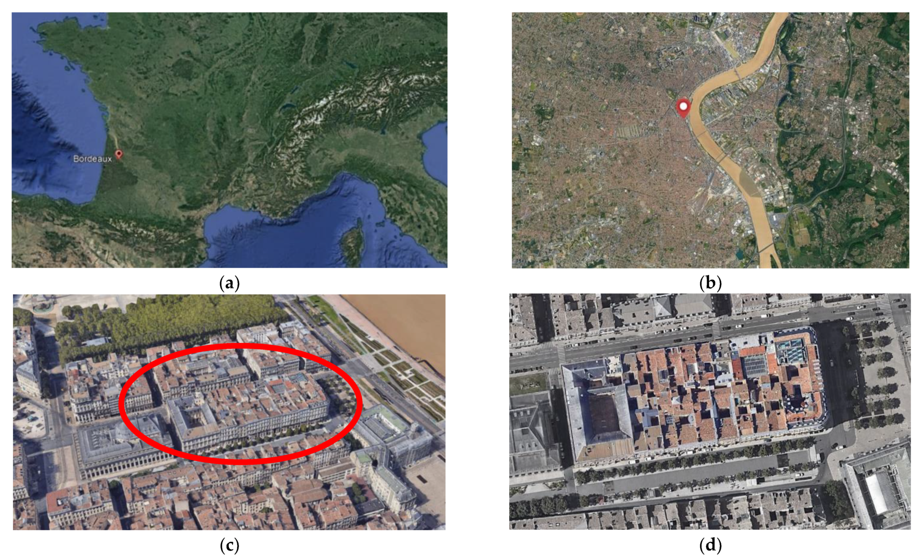
2.1. The Case Study

The modelling methods presented in this paper were applied to a particular and paradigmatic case study structure located in the city of Bordeaux, located in south-western France (Figure 1a,b). Bordeaux has an important historic urban centre built during the Enlightenment period, which was declared by UNESCO to be a World Heritage Site in 2007. The structure chosen as a case study (φ = 44°50′34″; λ = 0°34′19″) is located near the Grand Theatre de Bordeaux and is composed of at least 29 buildings (Figure 1c). The individual roofs of the buildings form a continuous roof of approximately 162 elements with some empty areas created by the interior gardens of the single buildings (Figure 1d). The roof and the façades present a certain intricacy of form where straight and curved elements are variously intersected. The geometries of these buildings lend themselves well to the application of the several 3D modelling methods proposed; therefore, this approach may also be extended to other structures of equal or greater complexity than those considered.

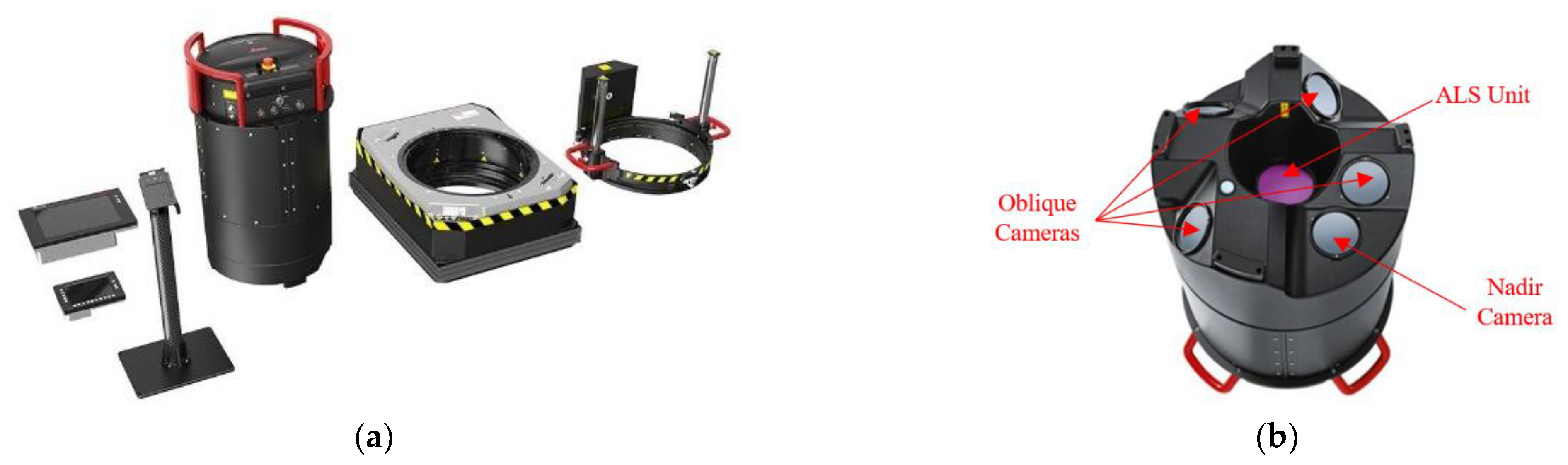
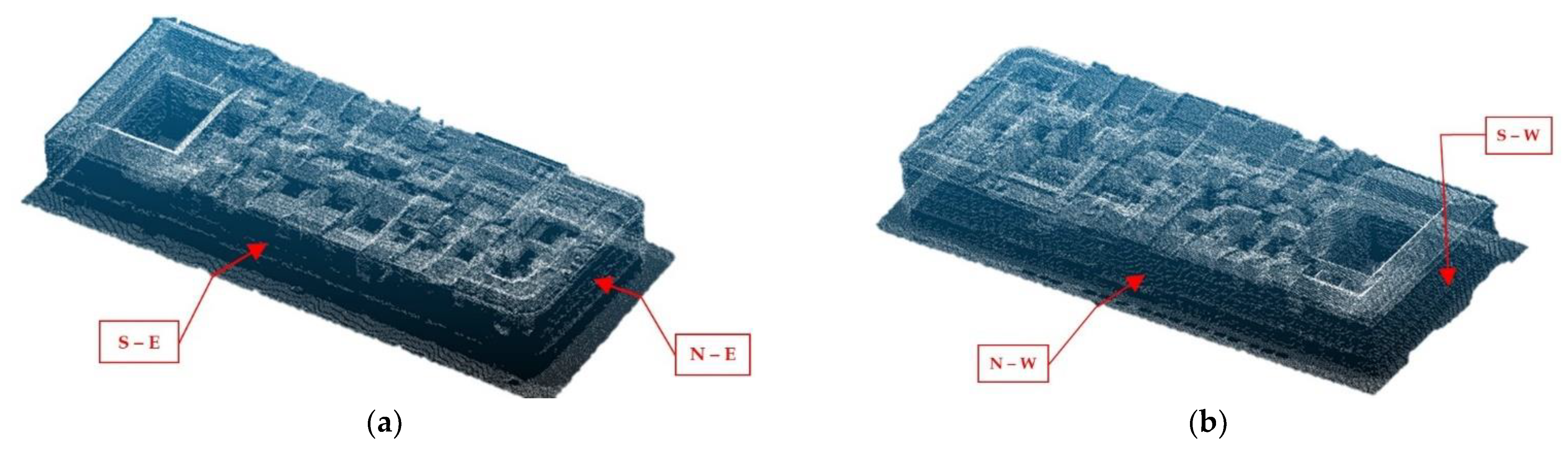
2.2. Dataset

The dataset used for the modelling of the structures is composed of a point cloud (generated by ALS sensors) and a dataset of colour images (generated by one nadir and four oblique cameras) [45]. For the data collection, a flight was carried out over the city of Bordeaux with a twin-engine aircraft (Partenavia P68C) at an altitude of 850 m above ground (850 m Average Ground Level—AGL) and using a “Leica CityMapper” hybrid sensor (Leica Geosystems AG—Part of Hexagon AB, Heerbrugg, Switzerland), which is specifically designed for airborne urban mapping (Figure 2).

The main data used in the geometric modelling of the structure is the point cloud (*.LAS) that was detected by the Leica Hyperion LiDAR ALS unit. The main features of the sensor are:

• Pulse repetition frequency up to 700 KHz;
• Return pulses programmable up to 15 returns, including intensity, pulse width, area;
• Under curve and skewness waveform attributes;
• Full waveform recording option at down-sampled rates;
• Oblique scanner, with various scan patterns;
• Real time LiDAR waveform analysis, including waveform attribute capture.

The survey produced a point cloud of 100,924 points (Figure 3), with a density on the horizontal surfaces (roofs and ground) of 7–8 pts/sqm and georeferenced in UTM Zone 30 North.

As can be seen in Figure 3, the density drops considerably on the vertical surfaces (the façades). The point cloud on the north-east (N-E) and south-east (S-E) façades (Figure 3a) is sparse while on the north-west (N-W) and south-west (S-W) façades (Figure 3b), it is sufficiently dense to be used for modelling.

The aerial images (Figure 4) were acquired by one Leica RCD30 CH82 multispectral nadir camera and four Leica RCD30 CH81 oblique cameras. The nadir camera uses a lens with an 83 mm focal length, while the oblique cameras use lenses with a 156 mm focal length. Nadir and oblique cameras use a 10,320 × 7752 pixels (80 MP) sensor. The flight plan on the Old Town Centre of Bordeaux was designed to obtain a Ground Sample Distance (GSD) of 5 cm for the nadir image.

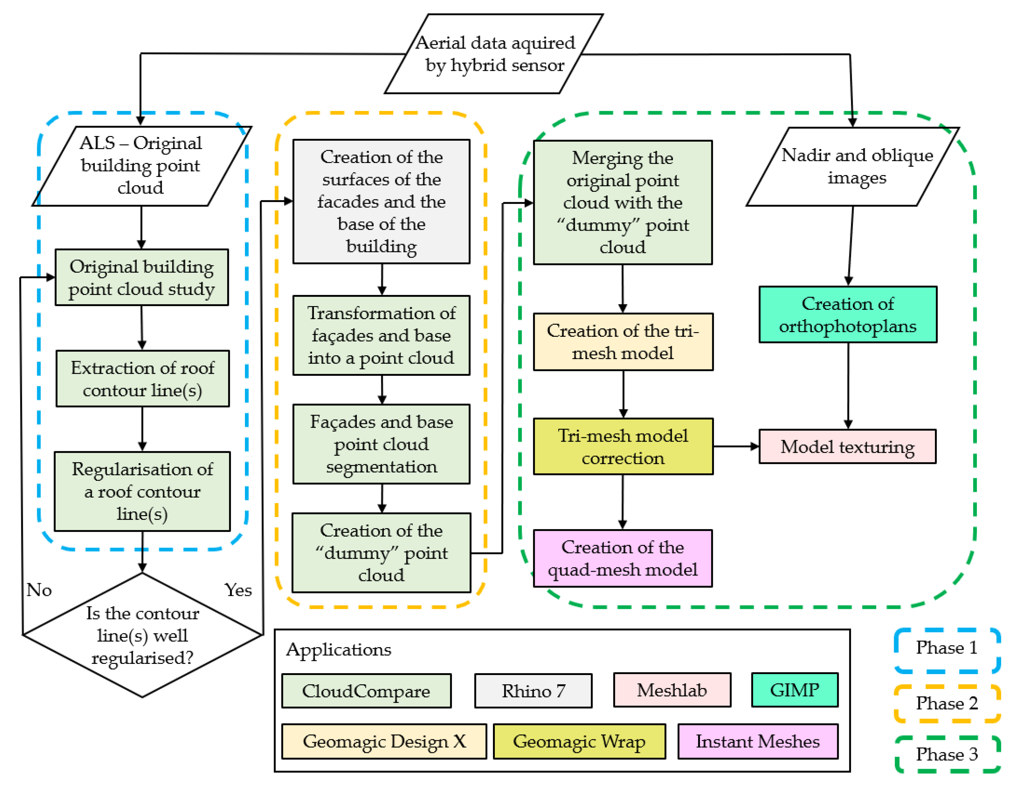
2.3. Data-Driven Free-Form Modelling

In the proposed data-driven free-form modelling method, the parts of the point cloud corresponding to the damaged N-E and S-E façades and the base were reconstructed by the creation of a supporting “dummy” point cloud. The roof and the N-W and S-W façades, where there was sufficient data for modelling, were preserved and modelled according to the input point cloud.

The pipeline of the developed method can be divided into three main phases, as shown in Figure 5.

The first step of the method (Phase 1) provides that contour lines of the roofs are extracted and regularised through iterative transformations from point cloud to mesh and vice versa. Subsequently, the polysurfaces of the façades and the base of the structure are created from the regularised contour lines (Phase 2). The polysurfaces are converted into a single point cloud and, through a segmentation and merging operation, the “dummy” point cloud is created. In Phase 3, the original point cloud and the “dummy” point cloud are merged. From the resulting point cloud, the triangular mesh (tri-mesh) model is created, and imperfections are automatically corrected. Finally, the tri-mesh model can be textured using nadir and oblique images or it can be transformed into a quadrangular mesh (quad-mesh) model.

The generated mesh model is based on the Poisson surface reconstruction method. In the most general form, proposed by Kazhdan et al. [23], given in input a point set S consisting of samples points s.p with s ∈ S and normal s.N facing inwards, which are assumed to be over or near a surface $\partial M$ of an unknown M solid model; the surface is reconstructed by solving a standard Poisson problem:

$$\mathsf{\Delta }\tilde{X}=\nabla ·\overrightarrow{V}$$

(1)

where $\overrightarrow{V}$ is the vector field and the gradient of the smoothed indicator function XM of M is equal to the vector field obtained by smoothing the field normal to the surface:

$$\nabla (X_M\ast \tilde{F})\left(q_0\right)={{\displaystyle \int }}_{\partial M}^{}{\tilde{F}}_p\left(q_0\right){\overrightarrow{N}}_{\partial M}\left(p\right)dp$$

(2)

where ${\overrightarrow{N}}_{\partial M}\left(p\right)$ is the inward surface normal in point $p\in \partial M$, $\tilde{F}\left(q\right)$ is a smoothing filter, and ${\tilde{F}}_p\left(q\right)=\tilde{F}\left(q-p\right)$ is the translation to the point p.

The surface integral cannot be solved since we do not know the geometric surface. So, the integral is approximated to the discrete summation. The approximation method consists of using the input point set S to divide ∂M into distinct patches $P_s\subset \partial M$, and then approximate the integral over a patch Ps at the value of the sample point s.p, scaled by the area of the patch:

$$\nabla (X_M\ast \tilde{F})\left(q\right)={\displaystyle \sum }_{s\in S}{{\displaystyle \int }}_{P_s}^{}{\tilde{F}}_p\left(q\right){\overrightarrow{N}}_{\partial M}\left(p\right)dp\approx {\displaystyle \sum }_{s\in S}\left|P_s\right|{\tilde{F}}_{s.p}\left(q\right)s.\overrightarrow{N}\equiv \overrightarrow{V}\left(q\right)$$

(3)

A graphic representation of the Poisson surface reconstruction method applied to a generic figure is given below (Figure 6).

The Poisson surface reconstruction method solves the Poisson problem for a watertight surface, so a failure to close the point cloud on the damaged façades and at the base, during processing with a surface reconstruction algorithm, would result in unacceptable artefacts that would be hard to modify automatically during post-processing.

Different tools and software were used for experimentation: CloudCompare (EDF R&D/TELECOM ParisTech ENST-TSI, Paris, France) [21], Rhinoceros^® (Robert McNeel & Associates, Seattle, Washington, DC, USA), Geomagic Design X and Geomagic Wrap (3D Systems, Rock Hill, SC, USA) [46], Instant Meshes (Interactive Geometry Lab, Zürich, Switzerland) [25], Meshlab (Visual Computing Lab—ISTI—CNR, Pisa, Italy) [22], and GIMP (The GIMP Development Team). As far as the hardware component is concerned, a PC with the following features was used: AMD Ryzen 7 4700U CPU, integrated Radeon Graphics 2.00 GHz GPU (Advanced Micro Devices, Inc., Santa Clara, CA, USA), and 16 GB of RAM.

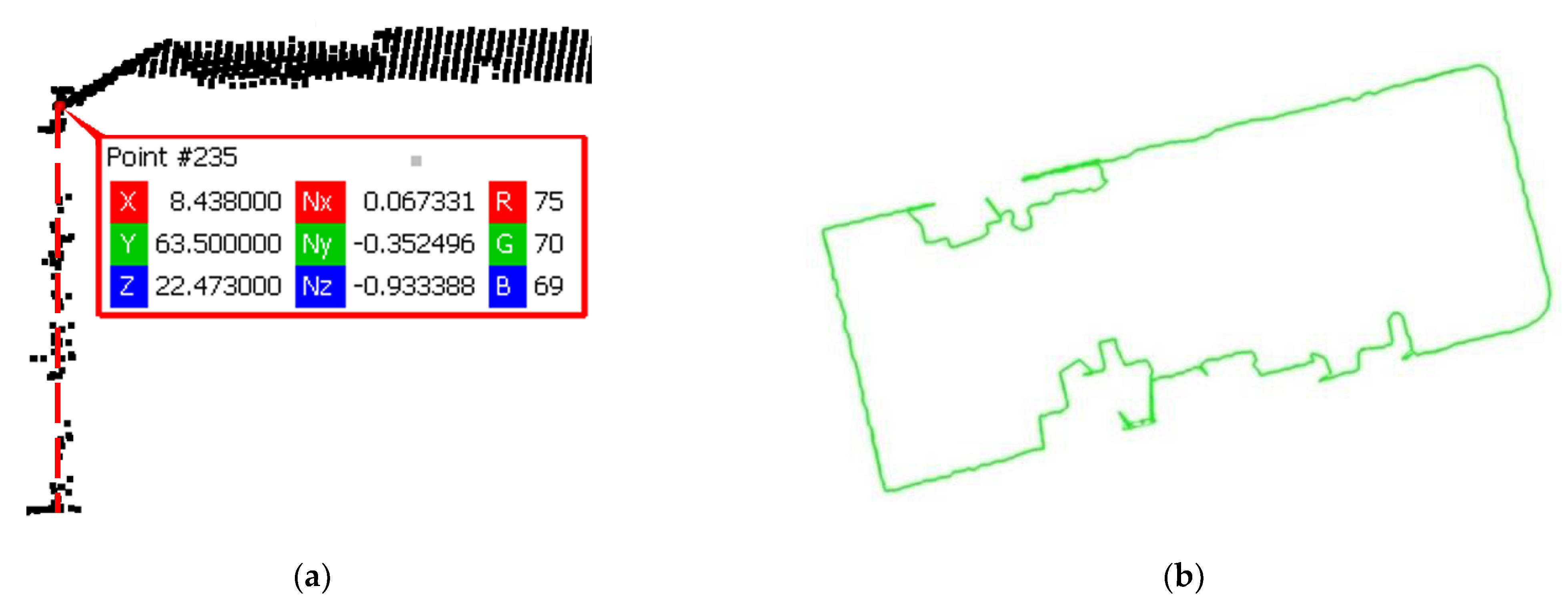
2.3.1. Phase 1: Extraction and Regularisation of Contour Lines

Once the point cloud was imported into CloudCompare software, it was possible to analyse features, such as spatial coordinates, colorimetric information, etc. (CloudCompare: Point picking); subsequently, we identified the parts of the roof where the contour lines could be extracted. In general, the criteria to be used to identify the part of the point cloud suitable for the extraction of contour lines are as follows: select the parts capable of generating sufficiently regular contour lines and the parts that allow for the contour lines produced to be aligned with the point cloud of the façades (Figure 7a). According to these criteria, a contour line inside the roof (line 1 Figure 7b) and a contour line at the eaves line (line 2 Figure 8a) were extracted. In the “Cross Section” tool, a Box Thickness of 1 m was set along the Z axis; in “Contour”, the “Contour type Full” was set; a value of 2.064 m was entered in “Max edge length”; and “project slice(s) points on their best fit plane” was selected.

Due to the density of the point cloud, the contour lines were irregular (Figure 8a) and in order to regularise contour lines, three operations were performed:

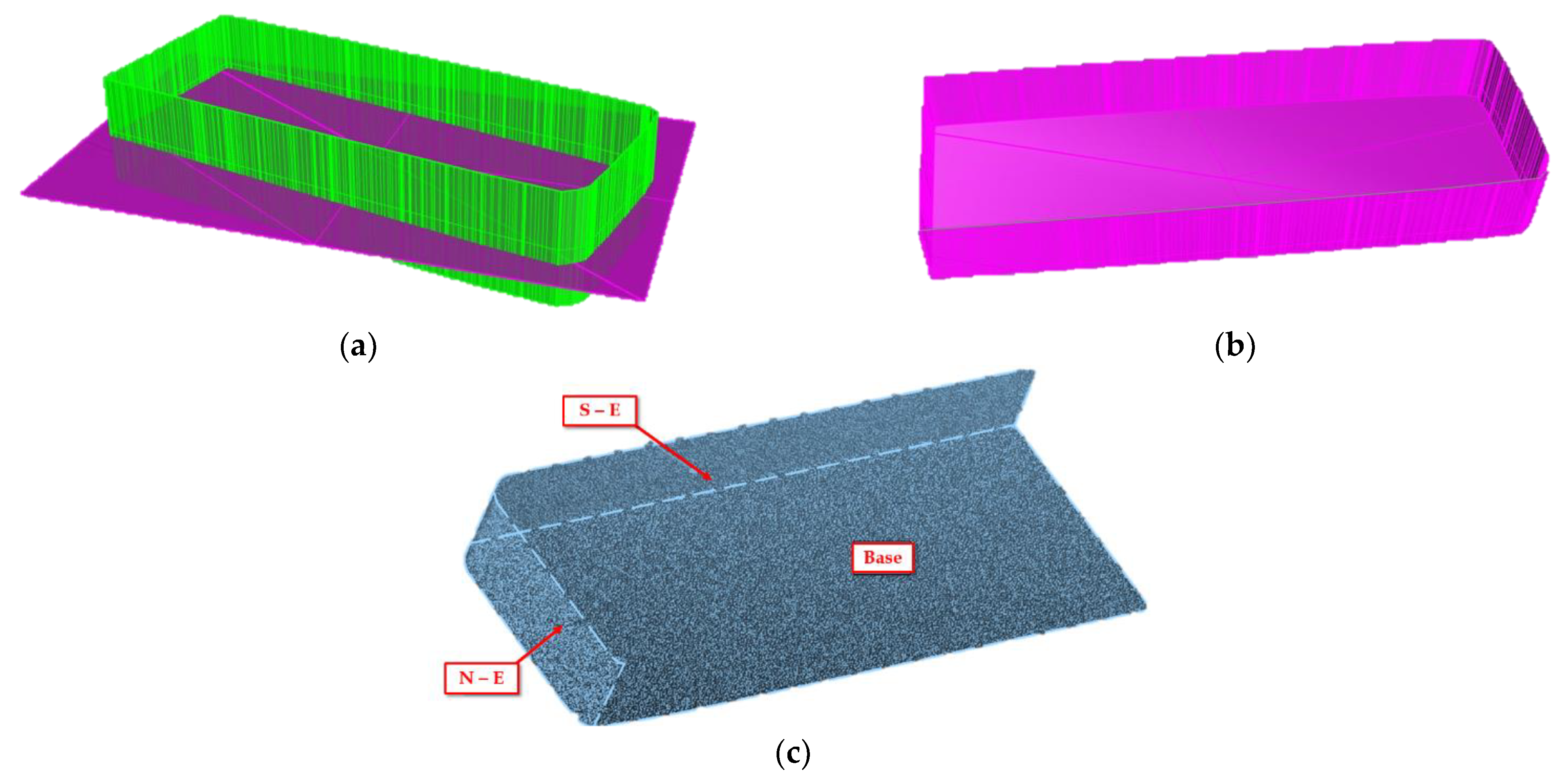
• Conversion of the contour line into a mesh plane (projection dimension: Z) where the contour line determines the edges of the output triangles (CloudCompare: Contour plot (polylines) to mesh—Figure 8b);
• Creation of a flat point cloud from the mesh surface (CloudCompare: Sample points on a mesh—Figure 8c);
• Extraction of a new regularised contour line from the flat point cloud (CloudCompare: Cross Section—Figure 8d).

At the end of these operations, we checked whether the contour line was regularised; if this was not the case, we repeated this operation iteratively.

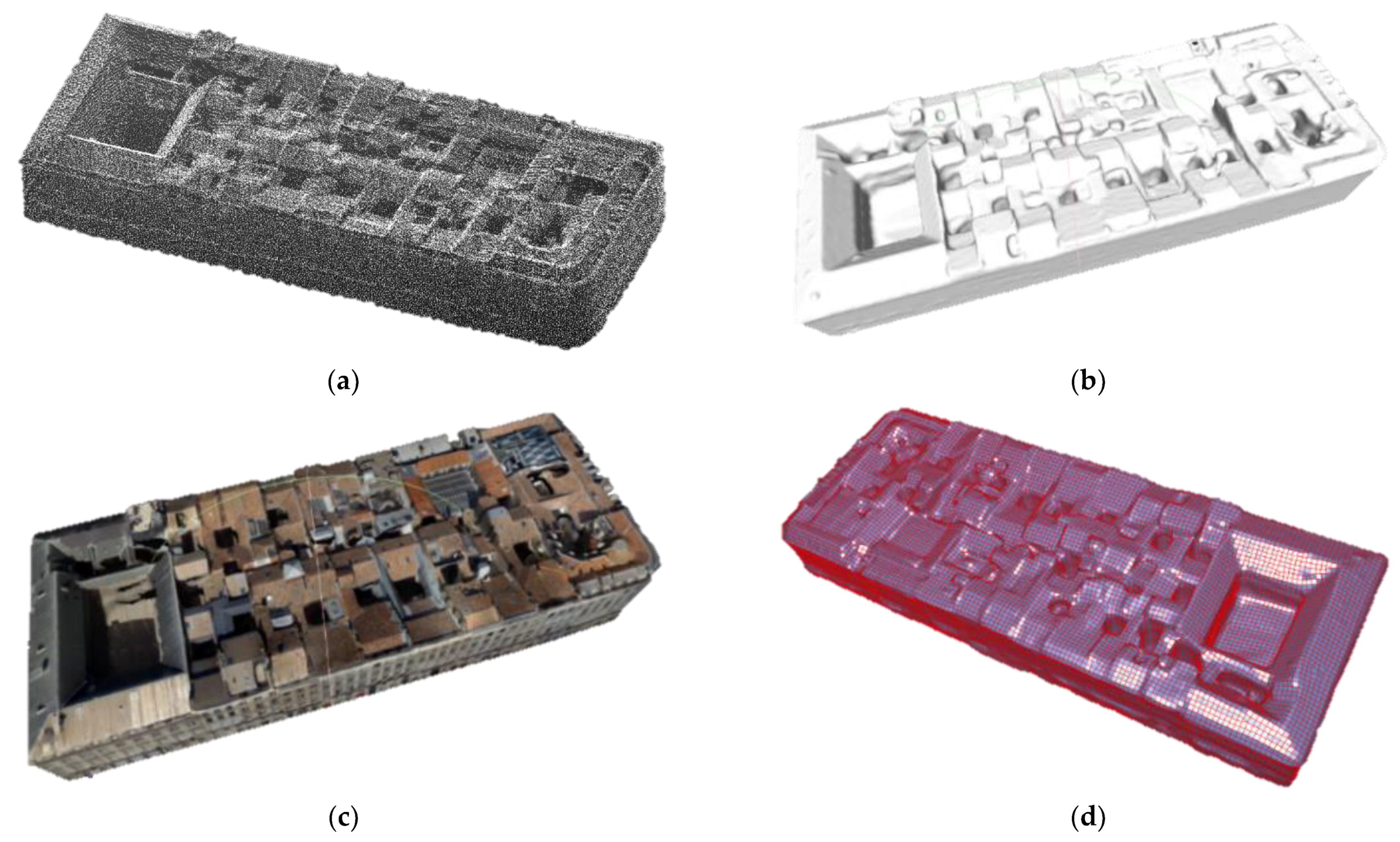
2.3.2. Phase 2: Creation of the “Dummy” Point Cloud

Contour line 2 was transformed into a point cloud (CloudCompare: Polyline, Sample points), and contour line 1 was cloned (CloudCompare: Clone) and shifted down along the Z-axis below the ground line generating contour line 3 (see Figure 9).

Using RanSac Shape Detection in CloudCompare [47], a mesh plane through the ground line was created. In RanSac Shape Detection, Plane was selected in “Primitives” and a value of 1000 was entered in “Min support points per primitive”. With RanSac Shape Detection giving a point cloud in input:

$$P=\left\{p_1,\dots ,p_n\right\}$$

(4)

With the normals associated:

$$N=\left\{n_1,\dots ,n_n\right\}$$

(5)

The algorithm of Schnabel et al. [47] provides in outputs a set of primitive shapes (plane, sphere, cylinder, cone, and torus):

$$\psi =\left\{{\psi }_1,\dots ,{\psi }_n\right\}$$

(6)

With the corresponding disjointed point cloud:

$$P_{\psi 1}\subset P,\dots , P_{\psi n}\subset P$$

(7)

As well as a set of remaining points:

$$R=P/\left\{P_{\psi 1},\dots ,P_{\psi n}\right\}$$

(8)

Contour line 1, contour line 3, and the mesh plane were imported into Rhino 7. The mesh plane was transformed into a polysurface (Rhino: MeshANurbs) and another polysurface was created between line 1 and 3, i.e., the façades indicated in green in Figure 10a (Rhino: Loft). By means of a Boolean operation, the polysurface of the façades was intersected with the polysurface of the ground; in this way, a 3D model consisting of the base and the façades was obtained (Figure 10b). In CloudCompare, the surface created in Rhino 7 was transformed into a point cloud (CloudCompare: Sample points on a mesh). In order to preserve the original point cloud of the N-W and S-W façades, it was necessary to segment the point cloud; this latter task was performed using RanSac Shape Detection implemented in CloudCompare. The segmented point cloud was reassembled (CloudCompare: Merge) and reconstructed (base, N-E, and S-E façades); the result of this operation was a “dummy” point cloud (Figure 10c). In this case, we selected (in RanSac Shape Detection) Plane in “Primitives” and entered a value of 100 in “Min support points per primitive”.

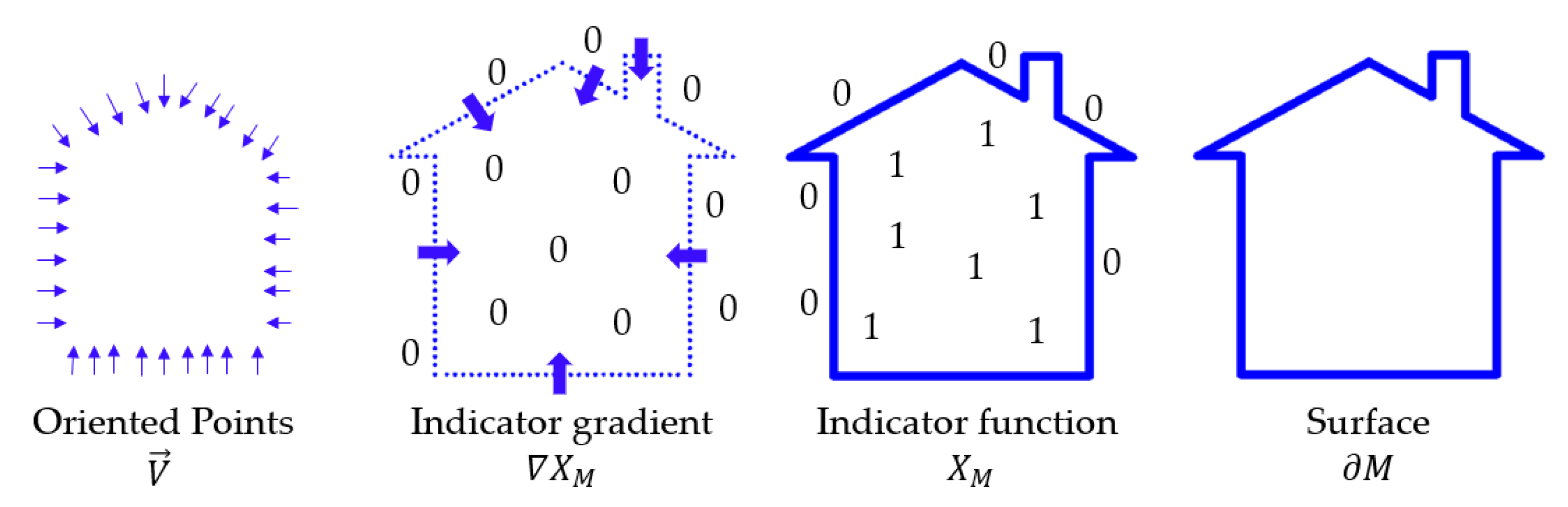
2.3.3. Phase 3: Generation of the Mesh Model

The original point cloud, the “dummy” point cloud, and the point cloud of the contour line 2 were merged (CloudCompare: Merge—Figure 11a).

In this case, the contour line 2 was used as a connection between roofs and façades. In general, the use of a connector is not mandatory and must be evaluated according to the case study.

The resulting point cloud was imported into Geomagic Design X. A “Cluster Filter” was applied to the point cloud in order to eliminate initial noise; for this reason, a value of 20 was set in “Max vertex count per cluster” (Geomagic Design X: Remove Noise). Subsequently, the triangular mesh model (tri-mesh) was generated by means of surface reconstruction (Geomagic Design X: triangulate) and after several tests, suitable values for the process of “HD mesh model”, “High definition filter”, “Noise reduction level”, “Extend contours to fill holes”, and “Shape of Filled area” were used.

The model generated in this way showed some imperfections; therefore, to improve its quality, the model was imported into Geomagic Wrap and corrected by removing non-manifold edges, self-intersections, high-fold edges, spikes, small components, small tunnels, small holes (Geomagic Wrap: Mesh Doctor), larger holes (Geomagic Wrap: Fill All), and smoothing the surface (Geomagic Wrap: Quicksmooth). The correct tri-mesh model is shown in Figure 11b.

Subsequently, the model was textured in Meshlab (Parameterization + texturing from registered raster) using the nadir and oblique images (Figure 11c).

Finally, the tri-mesh model was automatically simplified into a quadrangular mesh (quad-mesh) model with Instant Meshes; in this way, a lighter and more manageable 3D model for possible further processing was obtained (Figure 11d).

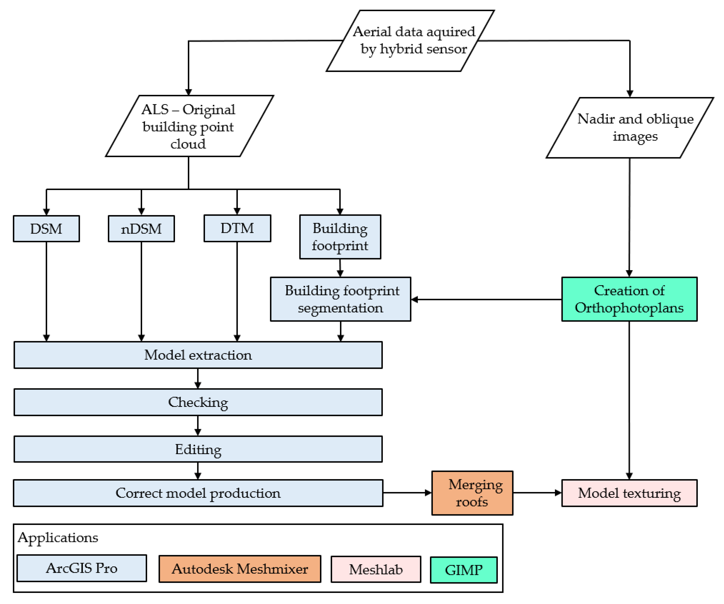
2.4. Model-Driven Modelling

Model-driven structure modelling was carried out using several software programs, such as 3D Basemaps Solution implemented in ESRI’s Arcgis Pro (ESRI, Redlands, CA, USA) [44], Whitebox Tools (Whitebox Geospatial Inc., Guelph, Ontario, Canada) [48], OpenStreetMap (OpenStreetMap Foundation, Cambridge, England, UK), Autodesk Meshmixer (Autodesk Inc., San Rafael, CA, USA), and MeshLab.

The quality of the 3D models is related to the density of the point cloud and the accuracy of the segmentation of the building footprint. In order to obtain satisfactory results, ESRI’s 3D Basemaps Solution requires an input point cloud with a point spacing of 1 metre or less; a recommended value for the spacing between points is 0.3 m. The point cloud taken into consideration respects the minimum value required and also the value recommended by ESRI.

To create a 3D model of the buildings, we need four input data: DTM, DSM, normalized Digital Surface Model, and nDSM and building footprint.

Figure 12 shows the building footprint segmentation based on the nadir images of the implemented method. To simplify the process of constructing the 3D model and, at the same time, increase the readability of the paper, only one of the six segmentation methods tested is shown in Figure 12. Since the geometry of the analysed structure is quite complex, the roofs were merged and, consequently, the final model could be textured by using nadir and oblique images.

In general, DTM, DSM, and nDSM can be derived even from external sources (e.g., the building footprint may be derived from a regional database). In this case, these geomatics data were automatically generated in 3D Basemaps starting from the point cloud (Figure 13) using two tasks: “Extract Elevation from LAS Dataset” (DTM, DSM, and nDSM) and “Extract building footprints” (building footprint).

The roof of the structure was very complex to be contained in the 3D Basemaps database; for this reason, to model the roof, it was necessary to apply the “divide and conquer” strategy. In this way, the entire roof was divided into a set of elementary roofs that could be recognized and modelled by 3D Basemaps.

In practice, we segmented the building footprint (Figure 13d) in order to separate contiguous buildings. 3D Basemaps was assigned a roof in the database to each individual building extracted from the segmented structure footprint.

In order to test how the segmentation modality affects the 3D model of the structure, we segmented the footprint in different modes:

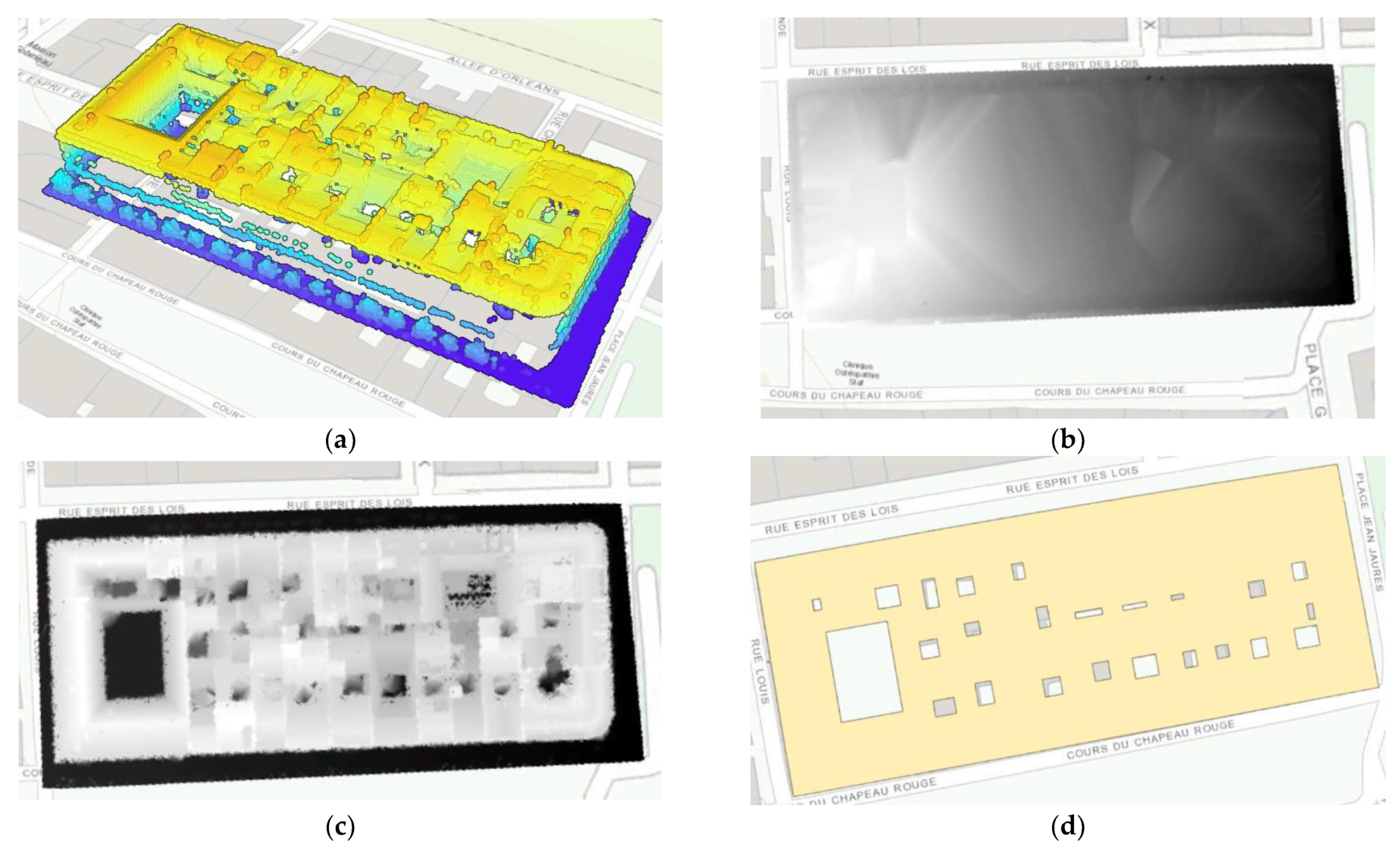
• Segmentation based on DSM;
• Segmentation based on the point cloud;
• Automatic segmentation based on nadir images;
• Segmented building footprint from OpenStreetMap—OSM;
• Segmentation based on the OSM features;
• Interactive segmentation based on nadir images.

A 3D model was automatically extracted from each segmented footprint, DTM, DSM, and nDSM (3D Basemaps: Create 3D Buildings). The models were numbered from 1 to 6 corresponding to the type of segmentation (Figure 14).

The models were analysed to determine the quality of the 3D model in relation to the segmented footprint building. In particular, in ArcGIS Pro software, the value of “RMSE” was verified, calculated between the model and DSM, and contained in the field of attribute tables of the 3D model generated in this environment.

In Cloud Compare software, the cloud-to-mesh distance (C2M) was performed.

Model 1 was derived from the building footprint segmented using DSM (3D Basemaps: Segment building footprints using elevation). The model has an RMSE of 3.641, a mean C2M of 1.254 m, and a C2M standard deviation of 1.725 m. The problem of this model is its inability to divide the model’s roof into elementary roofs (Figure 14b). This problem depends on the failure in segmenting the building footprint suitably (Figure 14a).

Model 2 was derived from the building footprint segmented using point cloud with Lidar Rooftop Analysis by Whitebox Tools. The model has an RMSE of 1.867, a mean C2M of 0.237 m, and a C2M standard deviation of 0.813 m. Because the segmented building footprint is fragmented (Figure 14c), this produces a model with fractured and irregular roofs, which is difficult to use for practical purposes (Figure 14d).

Model 3 was produced from the automatically segmented building footprint based on nadir image (ArcGis PRO: Segmentation). The model has an RMSE of 1.186, a mean C2M of 0.174 m, and a C2M standard deviation of 0.603 m. The problems of fragmentation and irregularities observed in model 2 are also observed in model 3.

Model 4 was extracted directly from the building footprint available in Open Street Map (OSM) [49,50,51,52,53]. The model has an RMSE of 2.679, a mean C2M of 0.240 m, and a C2M standard deviation of 1.200 m. The building footprint does not report all internal patios (Figure 14g) and this absence is reflected in the extracted model 4 (Figure 14h).

Model 5 was produced from a building footprint (Figure 14i) segmented using the OSM map as featured in 3D Basemaps (3D Basemaps: Split building footprints using features). The model has an RMSE of 2.060, a mean C2M of 0.266 m, and a C2M standard deviation of 1.040 m. Because model 5 can be considered as the union between model 1 and model 4, with this union it was possible to reconstruct some of the patios missing in model 4 (Figure 14j).

Model 6 was generated from the building footprint segmented interactively based on the nadiral image (Figure 14k) [12]. The model has an RMSE of 1.413, a mean C2M of 0.127 m, and a C2M standard deviation of 0.767 m. Model 6, with model 3, has the best combination of RMSE and C2M values, but some roofs were not modelled correctly by the software due to errors in the automatic recognition of the roof type. Compared to model 3, model 6 has no problems with fracturing and roof irregularities, and this makes model 6 better than model 3 (Figure 14l).

Therefore, the editing phase was applied to model 6 and two interactive editing operations were performed:

• Building footprint correction based on DSM (3D Basemaps: Modify Roof Tools);
• Parametric correction of the roofs through the modification of one or more fields of the attributes table (RoofForm, RoofDirAdjust, BldgHeight, EaveHeight).

The corrected model 6 has an RMSE of 1.167 and was renamed “model 7”.

This new model was built as a solid in Autodesk Meshmixer (Autodesk Meshmixer: Make Solid) to merge the various elementary roofs together and recreate the composite roof of the structure.

Subsequently, the model was textured in MeshLab like the tri-mesh model described in Section 2.3.3 (Figure 15).

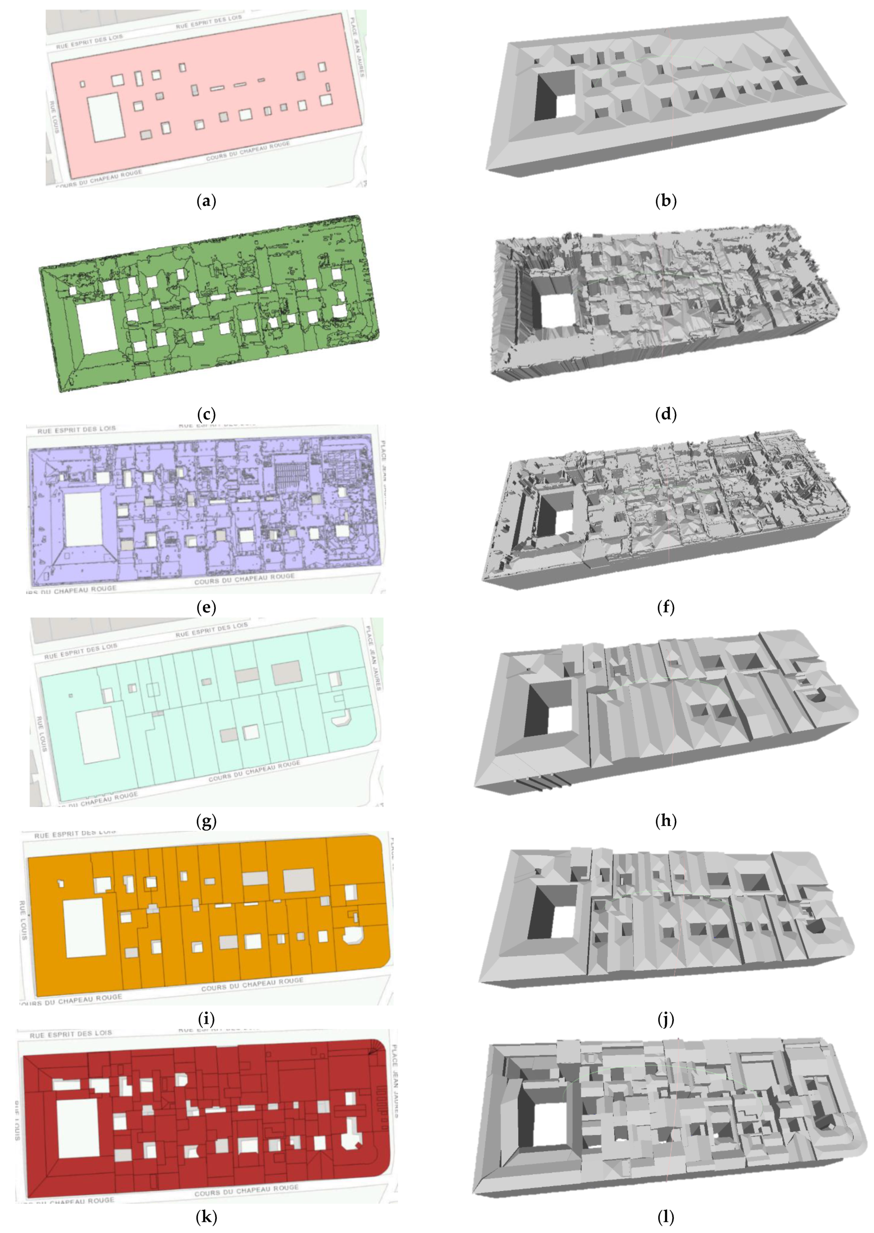
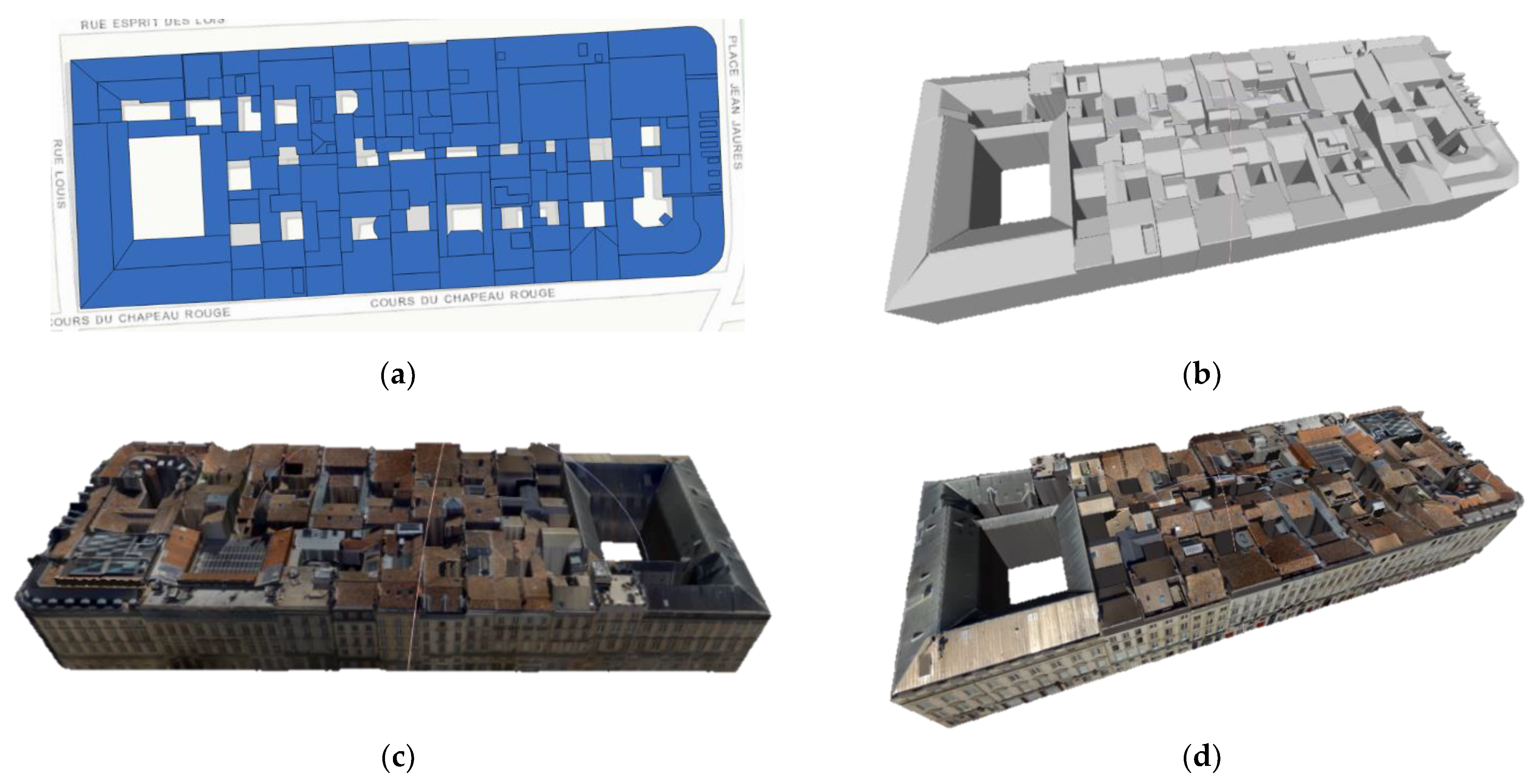
3. Results

In order to estimate the accuracy and precision of the models, we performed in CloudCompare software the Cloud to Mesh (C2M) distance between the original point cloud and the models created by the data-driven and model-driven methods.

Table 1. Mean and standard deviation values of the C2M distance of data-driven and model-driven models.

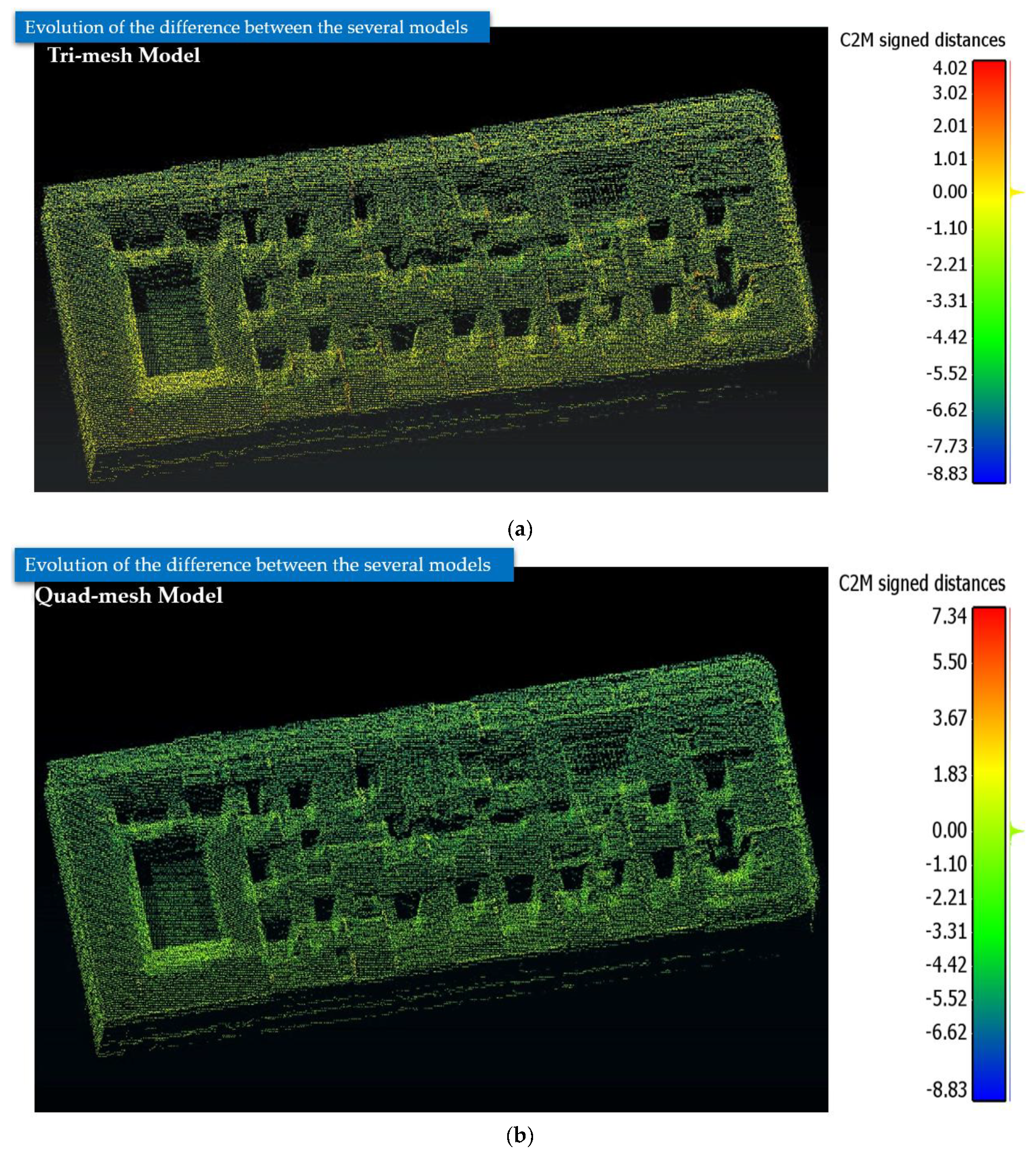
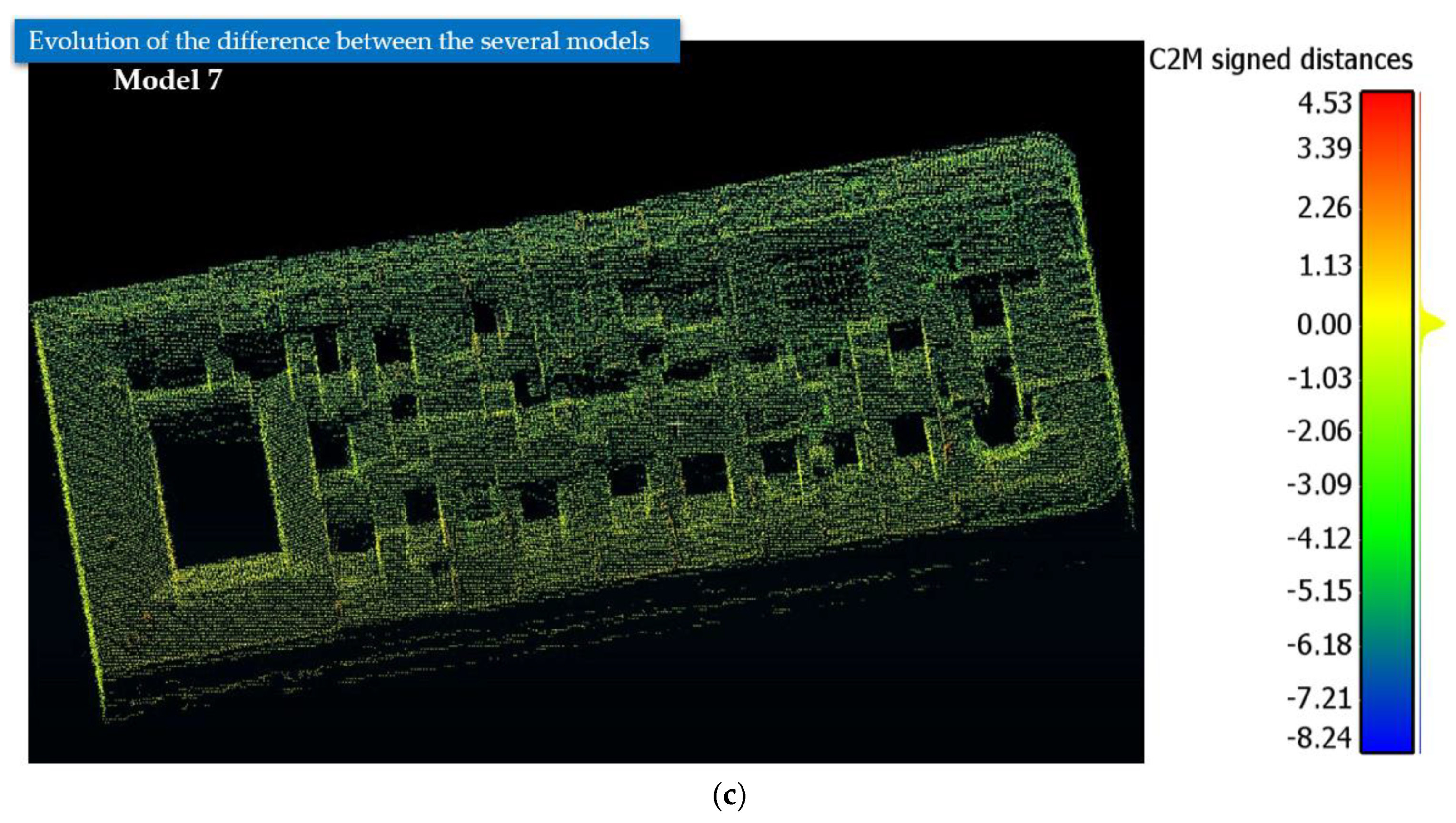
Modelling Type	Model	Formal Result	Mean C2M [m]	Standard Deviation C2M [m]
Data-driven free-form	Tri-mesh		0.066	0.612
	Quad-mesh		0.058	0.664
Model-driven	Model 1 (Segmented footprint based on DSM)		1.254	1.725
	Model 2 (Segmented footprint based on the point cloud)		0.237	0.813
	Model 3 (footprint automatically segmented according to nadir image)		0.174	0.603
	Model 4 (OSM footprint)		0.240	1.200
	Model 5 (OSM segmented footprint)		0.266	1.040
	Model 6 (footprint segmented interactively based on nadir image)		0.127	0.767
	Model 7 (interactive editing of the footprint and roof)		0.008	0.567

summarises the means and standard deviations of the Cloud to Mesh distances for all models.

In Appendix A, the results of tri-mesh, quad-mesh, and model 7 were reported for full reading. These latter 3D models showed the best values of the mean and standard deviation.

In addition, the simplification rate obtained by transforming a tri-mesh model into a quad-mesh model was assessed according to three reduction indicators: number of models vertices, number of model faces, and size of the files with the * PLY extension (expressed in kiloBytes).

Table 2. Simplification rate in the transformation from triangular mesh to quadrangular mesh.

Model	Vertices [n.]	Faces [n.]	Dimension [kB]
Triangular mesh	405,944	701,396	14,852
Quadrangular mesh	25,556	50,166	1012
Simplification rate	93.70 %	92.85 %	93.19 %

shows the results achieved in relation to triangular and quadrangular mesh; from the observation of this table, it is possible to note that for all three indicators taken into consideration, there is a simplification rate higher than 92%.

4. Discussion

The reconstruction of 3D models was achieved using various methods based on data-driven and model-driven modelling.

In the parametric reconstruction of complex structures and roofs, as shown in Table 1, the best results were obtained through the data-driven free-form method proposed (tri- and quad-mesh model).

The most significant technical aspects of the proposed method are:

• Regularisation of the roof contour lines by conversion into a mesh plane, in phase 1;
• Production of a “dummy” point cloud segmented according to the surveyed façades, in phase 2;
• Quad-mesh simplification as the preferred method for simplifying 3D models, in phase 3.

Regularization of contour lines through the conversion into the mesh plane is based on the principle of transforming convex parts of contour lines into plane edges and filling concave parts of contour lines with mesh triangles. Generally, smoothing algorithms are used to regularize the contour lines, but, in the case studied, the contour lines were too damaged for these methods (Figure 8a). However, using the method of conversion into the mesh plane, it was possible to reconstruct and regularise the contour lines of the roof (Figure 8d).

One of the most popular methods for reconstructing façades in 3D modelling using ALS data consist in the vertical extrusion of roof contour lines (e.g., using 3D Base-maps by ESRI). This method is very useful but when applied to historic buildings results in the loss of façade data. Instead, through the production of a “dummy” point cloud segmented and tailored specifically around the façades surveyed, it is possible to preserve, during the modelling phase, relevant data of the historical and artistically valuable façades.

During the research, various methods were tested to simplify the tri-mesh model: transformation into an NURBS model by Rhino 7, decimation of tri-mesh by Autodesk Meshmixer, and polygonisation by Geomagic Design X. All of these methods resulted in a loss of formal coherence of the model with a loss of roof definition. The method that produced the best results in the formal preservation of the 3D model was the transformation into a quad-mesh model with Instant Meshes. In addition, by observing and comparing the results reported in Table 1 and Table 2, it can be seen that a simplification of the tri-mesh model by more than 92% did not produce a significant loss of accuracy in the quad-mesh model. For these reasons, we believe that simplification by quad-mesh model transformation is preferable in the simplification of tri-mesh models of complex structures.

To investigate the limitations of modelling of complex structures by primitives, some modelling tests were performed using the Polyfit method. This method was able to model the structure as a simple prismatic shape. However, it is not possible to represent structures with a high degree of complexity. The data-driven free-form method proposed, instead, allows modelling of shapes with any degree of complexity.

An interesting point is the possibility of replacing, in the pipeline, the Poisson surface reconstruction method with the Delaunay method. To evaluate this possibility, we tried to model the original point cloud and the point cloud processed with the first two phases of the pipeline with the Delaunay method. In both cases, the result was a mesh model of the structure characterised by excessively irregular façades and a very noisy roof with many aberrations. These results were incompatible with the aims of the study conducted and for this reason, we do not recommend replacing the Poisson surface reconstruction method with the Delaunay method in this type of pipeline.

In order to evaluate the modelling limits in different operational scenarios (e.g., different areas, areas with modern buildings, natural areas, different countries, etc.) we produced four models named D.S. (Different Scenarios) and numbered from 1 to 4. D.S.1 is the model of a building with a multifaceted roof located at φ = 44°50′21″ and λ = 0°34′42″, model D.S.2 is derived from a modern building in Bordeaux located at φ = 44°50′9″ and λ = 0°35′15″, the building that generated the D.S.3 model has a layout similar to a triquetra and is located near Riverwalk Park in Naperville, Illinois (φ = 41°46′9″and λ = 88°9′33″), and D.S.4 was generated from a building with an interior patio located in the Naperville residential area (φ = 41°46′37″and λ = 88°9′2″).

The mean C2M and standard deviation C2M results are shown in Appendix B. Generally, the results are coherent with the results of tri- and quad-mesh models. In model D.S.2, we noted a difficulty of the method in reconstructing the technical installations located on the roof of the building.

We compared the results obtained with the results of Song et al. 2020. The results are shown in

Table 3. Comparison of free-form modelling methods.

Method	Model	Mean C2M [m]
Free-form modelling by Song et al., 2020	I	0.2749
	II	0.2777
	III	0.3312
	IV	0.3495
	V	0.1745
Free-form modelling proposed	Tri-mesh	0.066
	Quad-mesh	0.058
	D.S.1	0.029
	D.S.2	0.098
	D.S.3	0.088
	D.S.4	0.008

. The results, in this particular case study, are comparable to, if not better than, those obtained by those authors.

The model-driven method of 3D Basemaps (implemented by ESRI) gave the best results of C2M mean distance (0.008 m) and standard deviation (0.567 m) for Model 7. The method proposed in 3D Basemaps can be considered more efficient than the parametric free-form data-driven method if interactivity is included in the footprint segmentation phase and a final editing phase is added.

With regard to the automatic reconstruction of a complex roof using the model-driven method, it was noted that a segmentation of the footprint refined to the isolation of individual roof pitches does not automatically lead to an improvement in the model, since the application does not automatically recognise single-pitch roofs. This issue produces an error in the reconstruction of these roofs (e.g., shed roofs modelled as gable), which can only be resolved in an interactive way.

5. Conclusions

In this paper, we presented a free-form data-driven modelling method that aims to model buildings with complex shapes that are difficult to model automatically. The geodata used in this experimentation was obtained using a hybrid sensor, which is able to generate a georeferenced point cloud and produce nadir and oblique images. The proposed method was applied to some complex buildings located in the Old Town Centre of the city of Bordeaux, France.

The fundamental advantages of the proposed method are:

• Modelling buildings with any kind of shape using a parametric method;
• The possibility of choosing which building façades to model and which to reconstruct;
• To build photorealistic 3D models through the use of hybrid sensors;
• To obtain light and manageable 3D models without loss of accuracy and precision.

In order to present as complete a framework for modelling methods as possible, an analysis on the impact of footprint segmentation methods for buildings with complex roofs in model-driven modelling was performed. The segmentation was performed based on DSM, point cloud, nadir images, and OSM footprints. The comparison between the automatically extracted models shows that the building footprint segmentation that produces the most accurate model is the interactive segmentation based on nadir images. As shown in model 7, the model-driven method allowed a high level of accuracy to be achieved through the use of interactive editing.

By comparing the results obtained from the free-form data-driven models (tri- and quad-mesh) with automatically produced model-driven models (from one to six), it was shown that the best automatic method for reconstructing buildings with complex structures is the proposed free-form data-driven method. However, the 3D reconstruction of an entire city must take into account the geometry of the buildings, which can be either simple or complex. Therefore, it can be deduced that the best strategy for automatically modelling an entire city is to use the free-form data-driven method and the model-driven method together and sequentially.

According to this strategy, in the first step, large portions of the city (e.g., newly built districts) consisting of prismatic buildings and simple polyhedral buildings are automatically recognised and modelled with the model-driven method. Once the part of the city featuring simple geometries is modelled, in the second step, the complex buildings can be modelled in the data-driven free-form.

The proposed strategy allows the modelling of large urban areas (model-driven method) and the detailed reconstruction of complex shapes (free-form data-driven method).

References

- Biljecki, F.; Stoter, J.; Ledoux, H.; Zlatanova, S.; Çöltekin, A. Applications of 3D city models: State of the art review. ISPRS Int. J. Geo-Inf. 2015, 4, 2842–2889. [Google Scholar] [CrossRef] [Green Version]
- Bitelli, G.; Girelli, V.A.; Lambertini, A. Integrated Use of Remote Sensed Data and Numerical Cartography for The Generation of 3D City Models. Int. Arch. Photogramm. Remote Sens. Spat. Inf. Sci. 2018, 42, 97–102. [Google Scholar] [CrossRef] [Green Version]
- Pepe, M.; Costantino, D.; Alfio, V.S.; Angelini, M.G.; Restuccia Garofalo, A. A CityGML Multiscale Approach for the Conservation and Management of Cultural Heritage: The Case Study of the Old Town of Taranto (Italy). ISPRS Int. J. Geo-Inf. 2020, 9, 449. [Google Scholar] [CrossRef]
- Pepe, M.; Costantino, D.; Alfio, V.S.; Vozza, G.; Cartellino, E. A Novel Method Based on Deep Learning, GIS and Geomatics Software for Building a 3D City Model from VHR Satellite Stereo Imagery. ISPRS Int. J. Geo-Inf. 2021, 10, 697. [Google Scholar] [CrossRef]
- Wang, R.; Peethambaran, J.; Chen, D. Lidar point clouds to 3-D urban models: A review. IEEE J. Sel. Top. Appl. Earth Obs. Remote Sens. 2018, 11, 606–627. [Google Scholar] [CrossRef]
- Musialski, P.; Wonka, P.; Aliaga, D.G.; Wimmer, M.; Van Gool, L.; Purgathofer, W. A survey of urban reconstruction. Comput. Graph. Forum 2013, 32, 146–177. [Google Scholar] [CrossRef]
- Wang, R. 3D building modeling using images and LiDAR: A review. Int. J. Image Data Fusion 2013, 4, 273–292. [Google Scholar] [CrossRef]
- Haala, N.; Kada, M. An update on automatic 3D building reconstruction. ISPRS J. Photogramm. Remote Sens. 2010, 65, 570–580. [Google Scholar] [CrossRef]
- Brenner, C. Building reconstruction from images and laser scanning. Int. J. Appl. Earth Obs. Geoinf. 2005, 6, 187–198. [Google Scholar] [CrossRef]
- Shan, J.; Toth, C.K. Topographic Laser Ranging and Scanning: Principles and Processing, 2nd ed.; CRC Press: Boca Raton, FL, USA, 2018. [Google Scholar]
- Ebolese, D.; Dardanelli, G.; Lo Brutto, M.; Sciortino, R. 3D survey in complex archaeological environments: An approach by terrestrial laser scanning. Int. Arch. Photogramm. Remote Sens. Spat. Inf. Sci. 2018, 42, 325–330. [Google Scholar] [CrossRef] [Green Version]
- Buyukdemircioglu, M.; Kocaman, S.; Isikdag, U. Semi-automatic 3D city model generation from large-format aerial images. ISPRS Int. J. Geo-Inf. 2018, 7, 339. [Google Scholar] [CrossRef] [Green Version]
- Borrmann, D.; Elseberg, J.; Lingemann, K.; Nüchter, A. The 3d hough transform for plane detection in point clouds: A review and a new accumulator design. 3D Res. 2011, 2, 3. [Google Scholar] [CrossRef]
- Vosselman, G. Building reconstruction using planar faces in very high density height data. Int. Arch. Photogramm. Remote Sens. 1999, 32, 87–94. [Google Scholar]
- Maas, H.G.; Vosselman, G. Two algorithms for extracting building models from raw laser altimetry data. ISPRS J. Photogramm. Remote Sens. 1999, 54, 153–163. [Google Scholar] [CrossRef]
- Sohn, G.; Huang, X.; Tao, V. Using a binary space partitioning tree for reconstructing polyhedral building models from airborne lidar data. Photogramm. Eng. Remote Sens. 2008, 74, 1425–1438. [Google Scholar] [CrossRef] [Green Version]
- Dorninger, P.; Pfeifer, N. A comprehensive automated 3D approach for building extraction, reconstruction, and regularization from airborne laser scanning point clouds. Sensors 2008, 8, 7323–7343. [Google Scholar] [CrossRef] [Green Version]
- Nan, L.; Wonka, P. Polyfit: Polygonal surface reconstruction from point clouds. In Proceedings of the IEEE International Conference on Computer Vision, Venice, Italy, 22–29 October 2017; pp. 2353–2361. [Google Scholar]
- Bowyer, A. Computing dirichlet tessellations. Comput. J. 1981, 24, 162–166. [Google Scholar] [CrossRef] [Green Version]
- Watson, D.F. Computing the n-dimensional Delaunay tessellation with application to Voronoi polytopes. Comput. J. 1981, 24, 167–172. [Google Scholar] [CrossRef] [Green Version]
- Girardeau-Montaut, D. Cloud Compare; EDF R&D Telecom ParisTech: Paris, France, 2016. [Google Scholar]
- Cignoni, P.; Callieri, M.; Corsini, M.; Dellepiane, M.; Ganovelli, F.; Ranzuglia, G. Meshlab: An open-source mesh processing tool. In Proceedings of the Eurographics Italian Chapter Conference, Eurographics, Salerno, Italy, 1 January 2008; Volume 2008, pp. 129–136. [Google Scholar]
- Kazhdan, M.; Bolitho, M.; Hoppe, H. Poisson surface reconstruction. In Proceedings of the Fourth Eurographics Symposium on Geometry Processing, Cagliari, Italy, 26–28 June 2006; Volume 7. [Google Scholar]
- Kazhdan, M.; Hoppe, H. Screened poisson surface reconstruction. ACM Trans. Graph. (ToG) 2013, 32, 1–13. [Google Scholar] [CrossRef] [Green Version]
- Jakob, W.; Tarini, M.; Panozzo, D.; Sorkine-Hornung, O. Instant field-aligned meshes. ACM Trans. Graph. 2015, 34, 189:1–189:5. [Google Scholar] [CrossRef]
- Pepe, M.; Costantino, D.; Alfio, V.S.; Restuccia, A.G.; Papalino, N.M. Scan to BIM for the digital management and representation in 3D GIS environment of cultural heritage site. J. Cult. Herit. 2021, 50, 115–125. [Google Scholar] [CrossRef]
- Costantino, D.; Pepe, M.; Restuccia, A.G. Scan-to-HBIM for conservation and preservation of Cultural Heritage building: The case study of San Nicola in Montedoro church (Italy). Appl. Geomat. 2021, 1–15. [Google Scholar] [CrossRef]
- Schroeder, W.J.; Zarge, J.A.; Lorensen, W.E. Decimation of triangle meshes. In Proceedings of the 19th Annual Conference on Computer Graphics and Interactive Techniques, Chicago, IL, USA, 27–31 July 1992; pp. 65–70. [Google Scholar]
- Li, M.; Nan, L. Feature-preserving 3D mesh simplification for urban buildings. ISPRS J. Photogramm. Remote Sens. 2021, 173, 135–150. [Google Scholar] [CrossRef]
- Pepe, M.; Costantino, D. Techniques, tools, platforms and algorithms in close range photogrammetry in building 3D model and 2D representation of objects and complex architectures. Comput. Aided Des. Appl. 2020, 18, 42–65. [Google Scholar] [CrossRef]
- Zhou, Q.Y.; Neumann, U. 2.5D dual contouring: A robust approach to creating building models from aerial lidar point clouds. In European Conference on Computer Vision; Springer: Berlin/Heidelberg, Germany, 2010; pp. 115–128. [Google Scholar]
- Vo, H.T.; Callahan, S.P.; Lindstrom, P.; Pascucci, V.; Silva, C.T. Streaming simplification of tetrahedral meshes. IEEE Trans. Vis. Comput. Graph. 2006, 13, 145–155. [Google Scholar] [CrossRef] [Green Version]
- Ju, T.; Losasso, F.; Schaefer, S.; Warren, J. Dual contouring of hermite data. In Proceedings of the 29th Annual Conference on Computer Graphics and Interactive Techniques, San Antonio, TX, USA, 23–26 July 2002; pp. 339–346. [Google Scholar]
- Bouzas, V.; Ledoux, H.; Nan, L. Structure-aware Building Mesh Polygonization. ISPRS J. Photogramm. Remote Sens. 2020, 167, 432–442. [Google Scholar] [CrossRef]
- Song, J.; Wu, J.; Jiang, Y. Extraction and reconstruction of curved surface buildings by contour clustering using airborne LiDAR data. Optik 2015, 126, 513–521. [Google Scholar] [CrossRef]
- Song, J.; Xia, S.; Wang, J.; Chen, D. Curved buildings reconstruction from airborne LiDAR data by matching and deforming geometric primitives. IEEE Trans. Geosci. Remote Sens. 2020, 59, 1660–1674. [Google Scholar] [CrossRef]
- Lafarge, F.; Mallet, C. Creating large-scale city models from 3D-point clouds: A robust approach with hybrid representation. Int. J. Comput. Vis. 2012, 99, 69–85. [Google Scholar] [CrossRef]
- Rashidi, M.; Mohammadi, M.; Sadeghlou Kivi, S.; Abdolvand, M.M.; Truong-Hong, L.; Samali, B. A Decade of Modern Bridge Monitoring Using Terrestrial Laser Scanning: Review and Future Directions. Remote Sens. 2020, 12, 3796. [Google Scholar] [CrossRef]
- Mohammadi, M.; Rashidi, M.; Mousavi, V.; Karami, A.; Yu, Y.; Samali, B. Quality Evaluation of Digital Twins Generated Based on UAV Photogrammetry and TLS: Bridge Case Study. Remote Sens. 2021, 13, 3499. [Google Scholar] [CrossRef]
- Huang, H.; Brenner, C.; Sester, M. A generative statistical approach to automatic 3D building roof reconstruction from laser scanning data. ISPRS J. Photogramm. Remote Sens. 2013, 79, 29–43. [Google Scholar] [CrossRef]
- Poullis, C.; You, S. Photorealistic large-scale urban city model reconstruction. IEEE Trans. Vis. Comput. Graph. 2008, 15, 654–669. [Google Scholar] [CrossRef] [PubMed]
- Poullis, C.; You, S.; Neumann, U. Rapid creation of large-scale photorealistic virtual environments. In Proceedings of the IEEE Virtual Reality Conference, Reno, NV, USA, 8–12 March 2008; pp. 153–160. [Google Scholar]
- Henn, A.; Gröger, G.; Stroh, V.; Plümer, L. Model driven reconstruction of roofs from sparse LIDAR point clouds. ISPRS J. Photogramm. Remote Sens. 2013, 76, 17–29. [Google Scholar] [CrossRef]
- Sims, B.; Hedges, D.; van Maren, G. Creating and Maintaining Your 3D Basemap. In Esri User Conference Technical Workshops; ESRI: San Diego, CA, USA, 2017. [Google Scholar]
- Pepe, M.; Fregonese, L.; Crocetto, N. Use of SfM-MVS approach to nadir and oblique images generated throught aerial cameras to build 2.5D map and 3D models in urban areas. Geocarto Int. 2019, 1–22. [Google Scholar] [CrossRef]
- Li, Z.; Xiang, H.Y.; Li, Z.Q.; Han, B.A.; Huang, J.J. The research of reverse engineering based on geomagic studio. In Applied Mechanics and Materials; Trans Tech Publications Ltd.: Freienbach, Switzerland, 2013; Volume 365, pp. 133–136. [Google Scholar]
- Schnabel, R.; Wahl, R.; Klein, R. Efficient RANSAC for point-cloud shape detection. In Computer Graphics Forum; Blackwell Publishing Ltd.: Oxford, UK, 2007; Volume 26, pp. 214–226. [Google Scholar]
- Lindsay, J.B. The whitebox geospatial analysis tools project and open-access GIS. In Proceedings of the GIS Research UK 22nd Annual Conference, The University of Glasgow, GISRUK, Liverpool, UK, 16 April 2014; pp. 16–18. [Google Scholar]
- Girindran, R.; Boyd, D.S.; Rosser, J.; Vijayan, D.; Long, G.; Robinson, D. On the reliable generation of 3D city models from open data. Urban Sci. 2020, 4, 47. [Google Scholar] [CrossRef]
- Gröger, G.; Kolbe, T.H.; Czerwinski, A.; Nagel, C. OpenGIS® City Geography Markup Language (CityGML) Implementation Specification. 2008. Available online: http://www.opengeospatial.org/legal (accessed on 20 May 2021).
- Over, M.; Schilling, A.; Neubauer, S.; Zipf, A. Generating web-based 3D City Models from OpenStreetMap: The current situation in Germany. Comput. Environ. Urban Syst. 2010, 34, 496–507. [Google Scholar] [CrossRef]
- Fan, H.; Zipf, A. Modelling the world in 3D from VGI/Crowdsourced data. Eur. Handb. Crowdsourced Geogr. Inf. 2016, 435–446. [Google Scholar]
- Haklay, M.; Weber, P. Openstreetmap: User-generated street maps. IEEE Pervasive Comput. 2008, 7, 12–18. [Google Scholar] [CrossRef] [Green Version]