
Local Modal Frequency Improvement with Optimal Stiffener by Constraints Transformation Method

1
School of Astronautics, Beihang University, Beijing 100191, China
2
Beijing Institute of Spacecraft System Engineering, Beijing 100094, China
*
Authors to whom correspondence should be addressed.
Appl. Sci. 2021, 11(22), 11072; https://0-doi-org.brum.beds.ac.uk/10.3390/app112211072
Submission received: 19 October 2021
/
Revised: 10 November 2021
/
Accepted: 16 November 2021
/
Published: 22 November 2021
(This article belongs to the Special Issue Structural Vibration: Analysis, Control, Experiment, and Applications II)
Abstract
:Local modal vibration could adversely affect the dynamical environment, which should be considered in the structural design. For the mode switching phenomena, the traditional structural optimization method for problems with specific order of modal frequency constraints could not be directly applied to solve problems with local frequency constraints. In the present work, a novel approximation technique without mode tracking is proposed. According to the structural character, three reasonable assumptions, unchanged mass matrix, accordant modal shape, and reversible stiffness matrix, have been used to transform the optimization problem with local frequency constraints into a problem with nodal displacement constraints in the local area. The static load case is created with the modal shape equilibrium forces, then the displacement constrained optimization is relatively easily solved to obtain the optimal design, which satisfies the local frequency constraints as well. A numerical example is used to verify the feasibility of the proposed approximation method. Then, the method is further applied in a satellite structure optimization problem.
1. Introduction
The structural complexity of mechanical systems has significantly increased due to the increase of requirements in dynamic performance. Dynamic optimization has also become the most critical issue in structure design, especially for spacecraft structures with strict dynamic requirements [1]. As well known, satellite structures support all the functional components that are housed in it. If the natural frequency of the satellite structure overlaps with the frequency of excitation coming from the engine of launch vehicle, resonance will happen and high-amplitude vibration transmitting through the satellite structure will cause destruction to the payloads inside. Therefore, being one of the most important indicators of dynamic performance, the optimal design of structure with frequency constraint is extremely useful in manipulating the dynamic characteristics in a variety of ways. The ability to manipulate the selected frequency can remarkably improve the performance of the structure [2].
Many studies [3,4,5,6] related to the optimization of structures with frequency constraints are available. Du and Olhoff [7] considered different approaches for topology optimization involving simple and multiple eigenfrequencies. Yamada and Kanno [8] presented an algorithm with relaxation approach to solve the topology optimization with frequency constraints in frame structures. Li [9] studied the topology optimization with frequency band constraints for resonance avoidance. However, most of these papers consider a single or multiple frequency constraints in the general structural optimization, which use only the information about the global vibration frequency, such as the first-order lateral and the first-order vertical natural frequency. Few studies focus on local frequency requirements, which are sometimes also very important to improve the structural local stiffness for the key payloads installation areas.
There are no significant differences between the optimization problems with local and global frequency constraints [10]. One of the most intractable problems in local frequency optimization seems to be the switching of local modes due to structural size modifications [11]. The order of a certain local frequency is usually not constant and is hard to be identified automatically, especially during the structural optimization process, which will cause convergence difficulties to the optimizer [12,13]. Therefore, the method for structural optimization problems with global frequency constraints could not be directly applied in solving that with local frequency constraints.
Mode switching is the main problem in the process of dynamic structure optimization with local frequency constraints. Several survey papers in the field of local modes have been put forward. Tenek and Hagiwara [14] restricted the element density to a larger threshold to avoid local mode, which is why distinct gray areas showed in the optimization result of the material layout in the design of frequency maximization of dynamic structures. Pedersen [15] proposed an improved method of variable penalty factors to avert local mode SIMP. Cheng and Wang [16] put forward an approach to punish the element stiffness matrix of low-density areas by using polynomials. However, most of the presented works focus on the topology optimization for continuum structures, few works could be obtained for the sizing optimization problems.
In the present work, a new method is proposed to solve the structural optimization problem with local frequency constraints. In order to avoid the obstruction of mode switching, the essential idea of the new method is to transform the original structural dynamic optimization problem with local frequency constraints into an approximate static optimization problem with nodal displacements constraints. The nodal displacement constraints are derived by the initial modal shape of the local area and the ratio between the initial local frequency and the expected local frequency. A numerical example is used to verify the feasibility of the proposed approximation method. Then, the method is further applied in satellite structural optimization problem.
2. Problem Formulation
The dynamic structural optimization problem with frequency constraint to be solved is: find the set of design variables that will minimize the objective with local frequency constrained to a required value, which can be formulated as follow.
where the mass of the structure, , is taken as the objective function. The constraint, , is about the local frequency, is the local frequency in the initial design, is the local frequency in the optimal design, and is the magnification of the constrained local frequency. and are the corresponding lower and upper limits on , and is the number of design variables.
It is a common practice that available reinforcement structures are added in local area to enhance the rigidity, as well as the local mode frequency. Therefore, in our optimization problem, the dimension parameters of the reinforcement structures are treated as design variables.
3. Optimization Strategy
As already mentioned in the introduction, because of the serious mode-switching phenomenon of local mode, it becomes especially complicated to determine the optimum when taking the local frequency constraint into consideration. The typical optimization process is not suitable for optimization with a local frequency constraint. Accordingly, we proposed an approximate method using the information of nodes displacements in local areas to be optimized, which avoids using the order of the local mode and its identification.
3.1. The Three Assumptions
First of all, according to the structure model and optimization problem, three assumptions have been used to guarantee an accurate and reasonable transformation process of the displacements constraint from the local frequency constraint. The three assumptions are as follows.
Assumption 1.
During the process of optimization, the dependence between design variables and mass matrix is small enough to the neglected.
Assumption 2.
The modal shape of the specified local frequency is accordant before and after optimization, that is , is the modal eigenvector.
Assumption 3.
There is no rigid body mode in the structure, which means that the element stiffness matrix of the structure is reversible.
3.2. Equilibrium Forces
An essential point for the local frequency constraint transformation is to establish the static load case.
Since the gained weight of reinforcement structural is small relative to the weight of original structure, there is little to no impact in the element mass matrix, which corresponded to Assumption 1. However, structural modification has a major impact on the element stiffness and the change in it should not be overlooked [17]. Therefore, the stiffness matrix is assumed to be a linear function of design variables in optimization problem.
when analyzing the dynamics of an undamped structure, the characteristic equation can be expressed in the following matrix form
where is the natural frequency or eigenvalue of the i-th mode, and is the corresponding natural modal shape or eigenvector.
The mode of the normalization of the mass matrix can be expressed as
According to Equation (3), considering the local mode of initial design, it can be written as
where is the element stiffness matrix of the initial design. Similarly, considering the local mode of current design, the equation can be written as
where is the element stiffness matrix of the current design and the mass matrix remains constant.
According to Assumption 2, Equation (6) can be expressed as
Combining Equations (5) and (7), and removing the common item from both equations, we can further relate the element stiffness matrix in the initial and current design as
To further transform the modal frequency information, reading the specified local modal shape for reference, we can define a virtual equivalent external load as
when the modal analysis of the initial structure is conducted, the equivalent external load can be obtained as well.
3.3. Transformation into Displacement Constraints
With applied to the structure of current design, the static analysis, formulation can be expressed as
where is the vector of nodal displacements. Substitution of Equation (9) into Equation (8) gives the expression
Substitution of Equation (10) into Equation (11) gives the expression
According to Assumption 3, that matrix has inverse matrix, the two ends of Equation (14) are multiplied by . Then, we obtain the relationship between the nodal displacements and the local frequency
Here, the relationship can be used for the transformation. According to the frequency constraints in Equation (1), that is
Substitution of Equation (13) into Equation (14) gives the expression of nodal displacement constraint
At this point, the frequency constraints of the original problem can be transformed into the displacement constraints of the approximate problem.
It can be evidenced from the final that the displacements of each node of the structure are required to be constrained, which brings a lot of work on the establishment of the approximate optimization model as well as the complexity of problem-solving. However, the nodal displacements of the structure mean the same as the modal shape of the structure. That is to say, for local vibration mode, the relatively obvious nodal displacements are almost limited in local vibration area. Thus, as a reasonable simplification approach, the nodal displacements in local vibration area are only constrained in establishing the approximate optimization model.
3.4. Optimization Model with Displacement Constraint
With the transformed constraint, the approximate optimization model for the current approximation can be stated as follows: find the set of variables that will minimize structural weight with the nodal displacements constraints and the equivalent external load applied, expressed as
where the mass of the structure, , is taken as the objective function. The constraint, , is transformed the local frequency constraint, is the local modal shape in the initial design, is the vector of nodal displacements, is the magnification of the constrained local frequency. and are the corresponding lower and upper limits on , and is the number of design variables.
The approximate optimization model is no longer affected by local mode. That is to say, the local mode switching phenomenon will not alter the constraints in the optimization model. Instead, the static analysis with the equivalent external load is needed.
4. Approximate Optimization Process
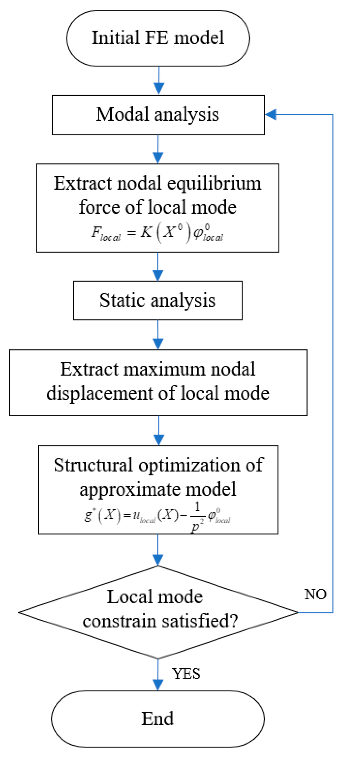
An outline of the optimization process using the approximation method is given as follows:
- Establish the initial FE model and perform a detailed mode analysis to get and ;
- Extract the nodal equilibrium forces of local vibration mode from mode analysis results, ;
- Establish a static load condition according to above-obtained nodal equilibrium forces and perform a static analysis;
- Extract the maximum nodal displacement from static analysis results;
- Create a high-quality approximation using the aforementioned information and then perform the optimization with constraint, ;
- Update the analysis model and perform a complete analysis. Check for convergence to an optimum. If satisfied, terminate. Otherwise, repeat from step 2.
Repeat steps 2–4 until the convergence requirements are satisfied. Steps 2–4 constitute one iteration. The flow chart shown in Figure 1 illustrates the proposed approximate method.
We need to mention at this point that in order to obtain a high-quality optimization, artificial modeling is required. Due to part of the needed date, the orders of the local mode, for instance, must be manually selected. How to obtain the nodal equilibrium forces of local mode and establish static load condition in FE model are two difficult and important issues in artificially forming the approximation. Here, we accomplish both operations with the help of Msc. Patran/Nastran. In the software, the Grid Point Force Balance is optional in the output request of mode analysis subcase, which is the virtual equivalent load in Equation (9). With the Grid Point Force Balance information, we can establish static load with fields table node by node.
5. Numerical Examples
On the basis of the numerical procedure presented in the previous section, two numerical examples were conducted to verify applicability, effectiveness, and accuracy of the approximation method. The first example was inspired by an example in Reference [15] by Pedersen. The second example was a practical optimization problem of a large-scale satellite.
In the following examples, emphasis is placed on the change in the theoretical magnification of the constrained local frequency, , relative to the practical magnification calculated with the optimization result, . Thus, in each example, variation from the relative error was a measure of the accuracy of the approximate method.
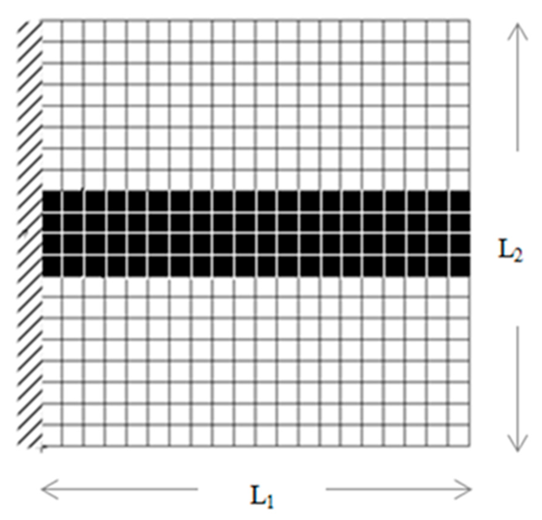
5.1. Example 1: Thin Plate
As described in Reference [15], the minimum structural weight of the plate was to be found with the local frequency constrained to be not lower than 60 Hz. The FE model of the plate clamped at one end is shown in Figure 2, and it used a total of 20 × 20 elements of 50 × 50 mm. The left side of the plate was fixed, and the materials in the white area and the black area were and , respectively, shown in Table 1. The dimensions of the plate were L1 = 1 m, L2 = 1 m and the thickness T = 0.02 m.
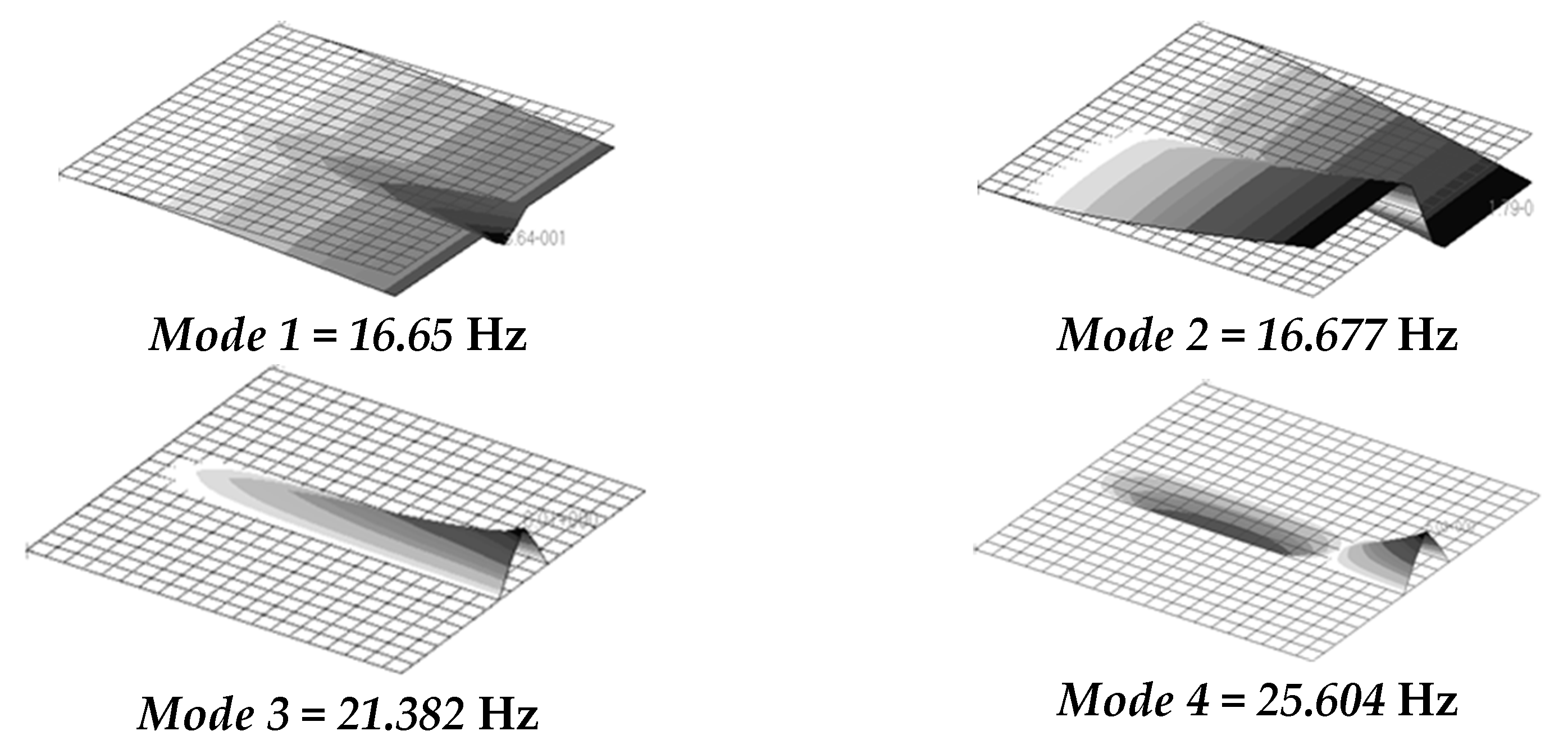
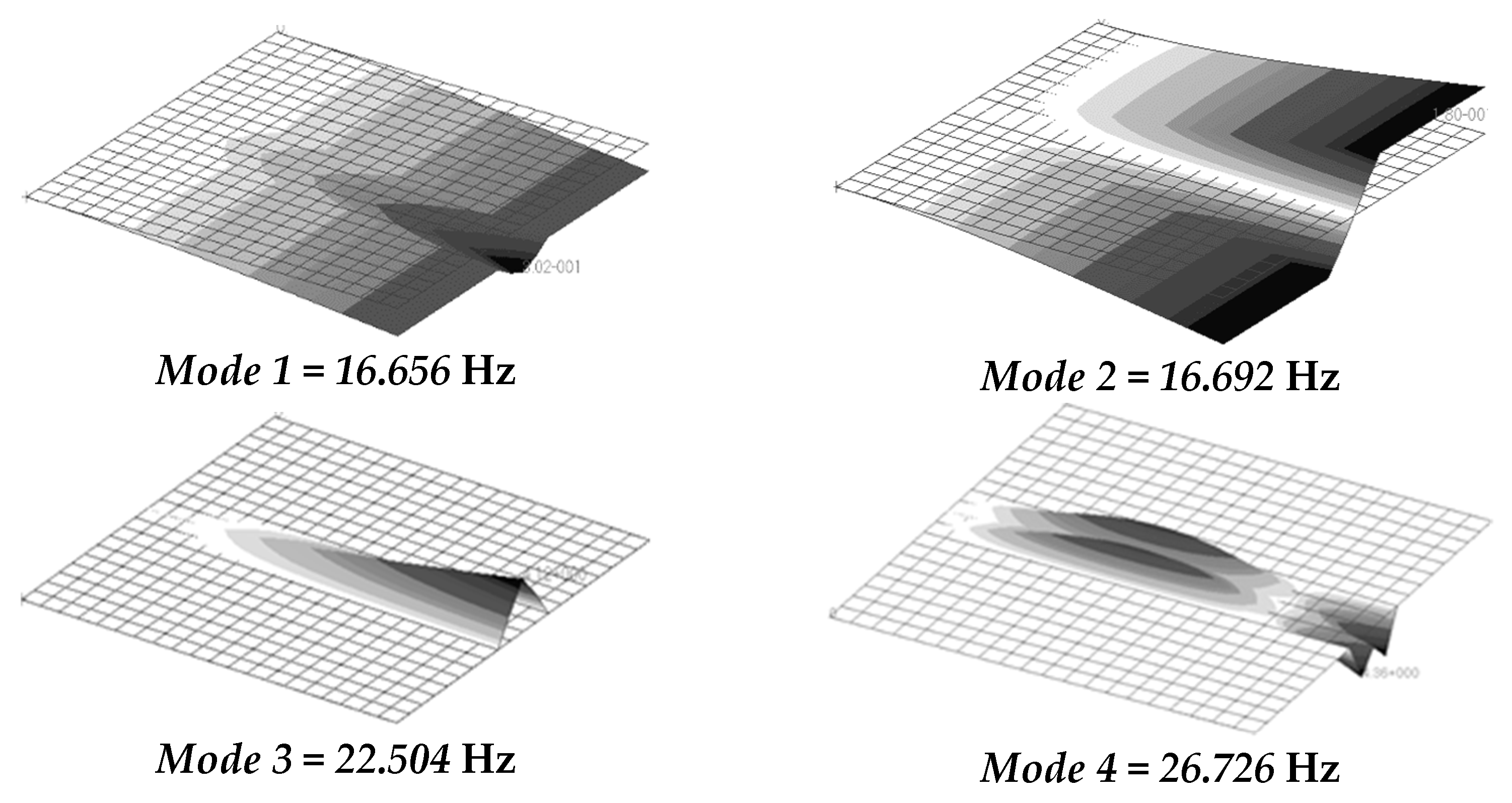
The first four orders of natural frequencies and modal shapes of the initial plate are shown in Figure 3. It was obvious that the third order mode was the local mode of the initial plate and the initial local frequency was 21.382 Hz.
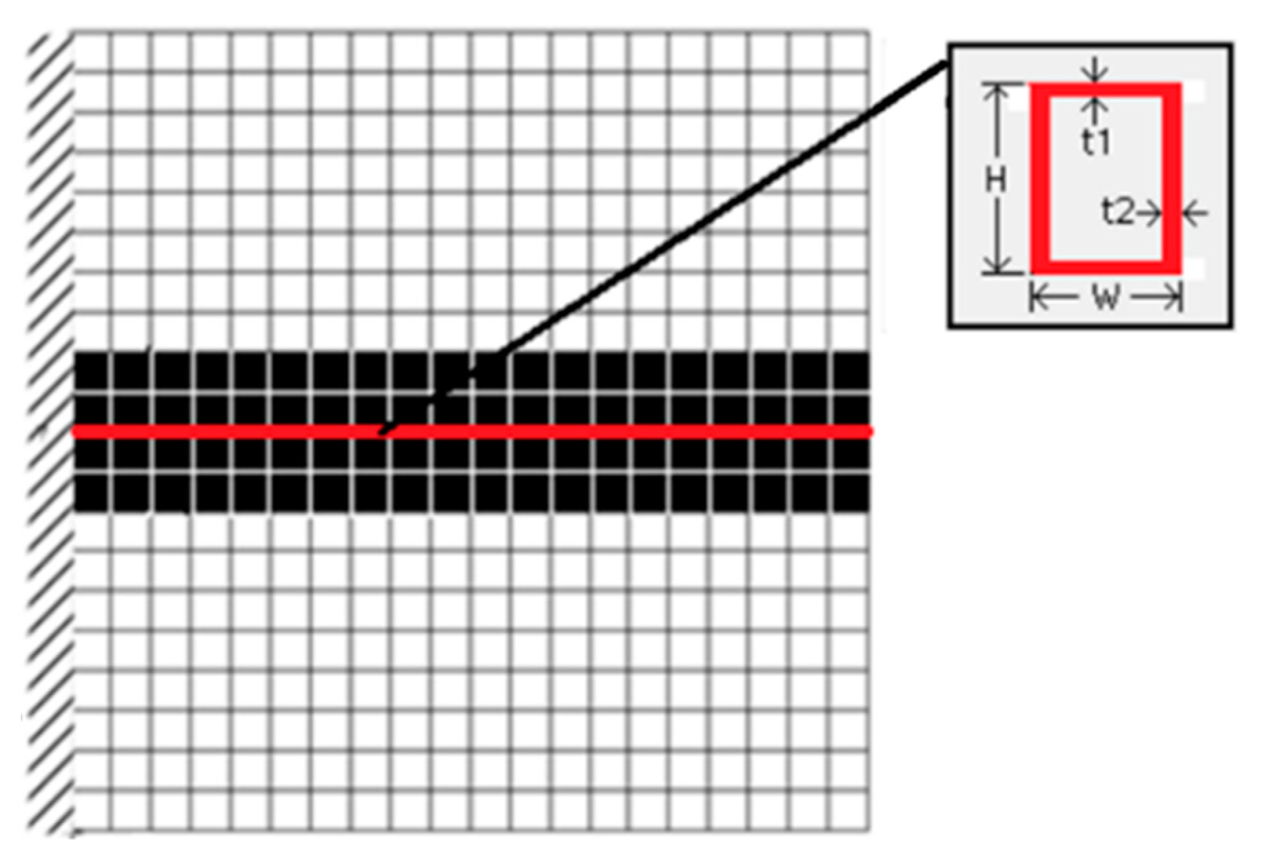
A reinforced stiffener, whose cross section is shown in Figure 4, was placed where the maximum displacement occurred to improve the local frequency. The initial design was H = W = 0.01 m and t1 = t2 = 0.002 m.
Performing a modal analysis and the first four orders of the natural frequencies and modal shapes of the plate with the reinforced stiffener is shown in Figure 5. The natural frequencies changed slightly and the third order mode was also the local mode. In this way, modifying the design of the cross section to satisfying the local frequency constraint with the minimum mass increasement was the optimization problem.
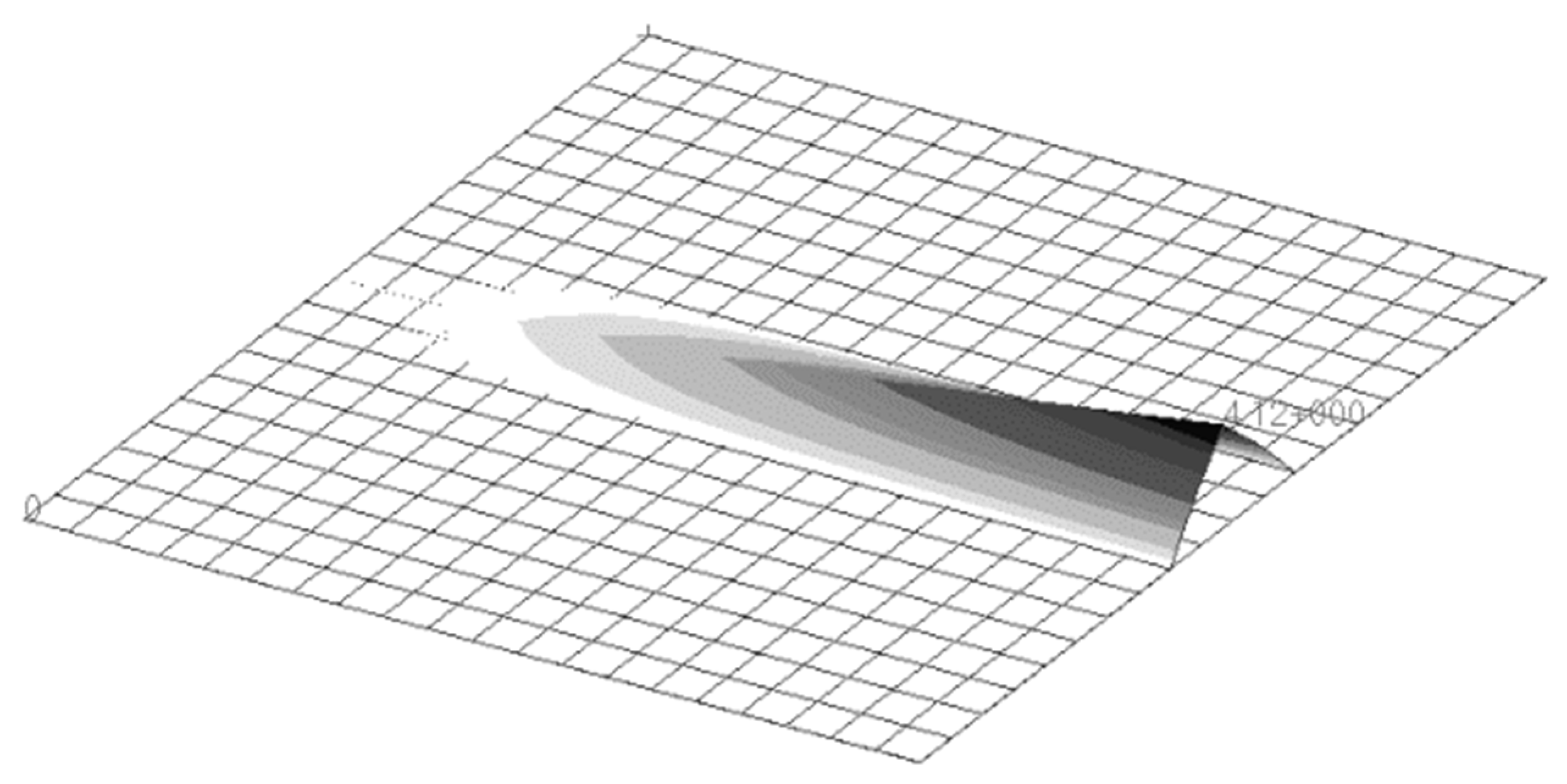
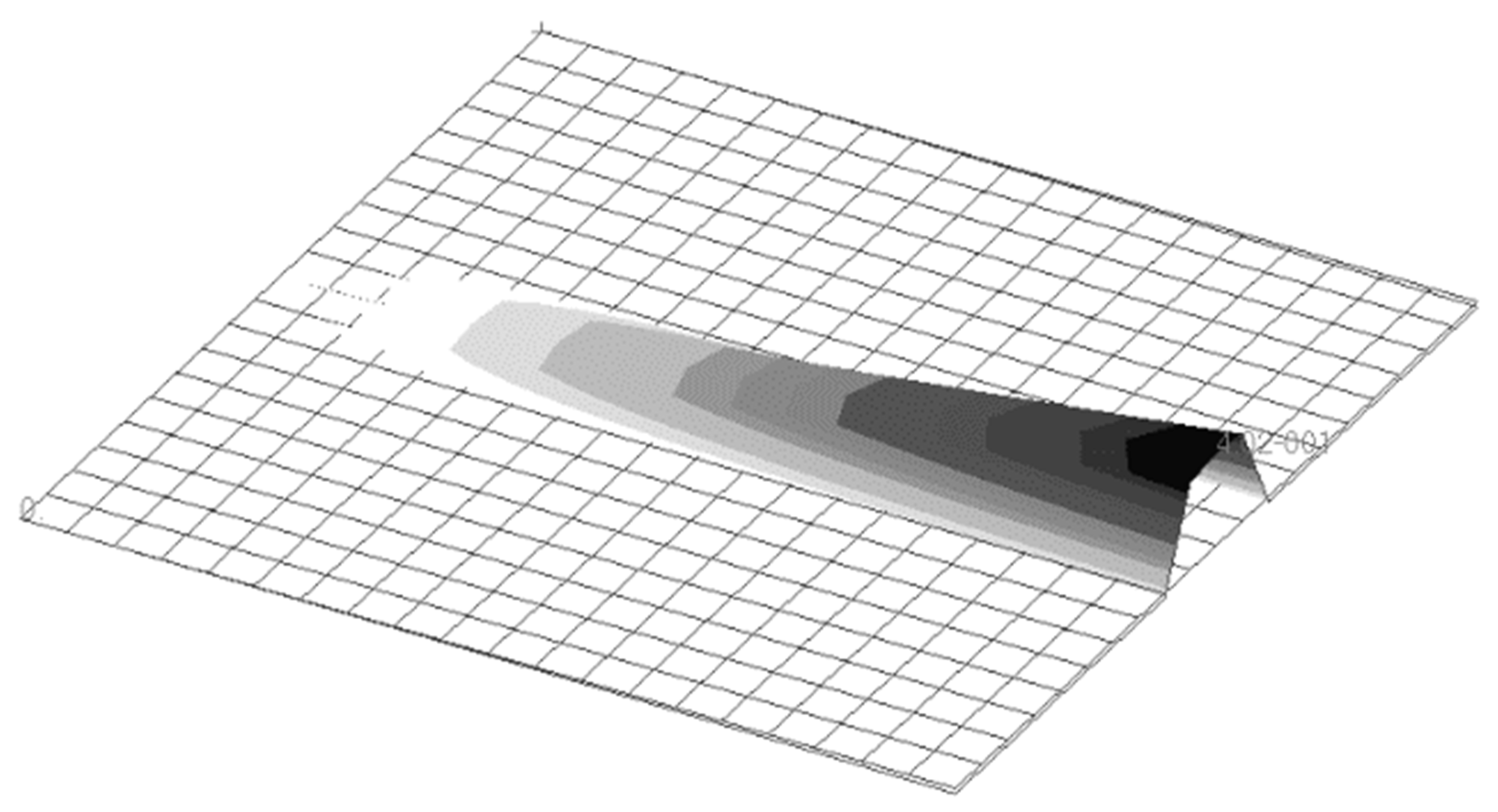
The nodal equilibrium forces of the local mode was obtained directly from the modal analysis, and what followed was to establish a static load condition according to above-obtained forces. Then, we continued the static analysis based on the above-established load condition. It was apparent that the nodal displacements from the static analysis shown in Figure 6 were consistent with the third order modal shape from the modal analysis shown in Figure 5, conforming to the assumptions made when defining static loads.
The approximate optimization model was then established with the objective of structural mass, the design variables of cross-section dimensions shown in Table 2, and the constraint of nodal displacement. In the initial optimization problem, the local frequency was constrained to be not lower than 60 Hz, and the nodal displacements could also be calculated by Equation (16) accordingly. Therefore, in the approximate problem, the magnification of the constrained local frequency was , the nodal displacements on the reinforced stiffener were constrained less than .
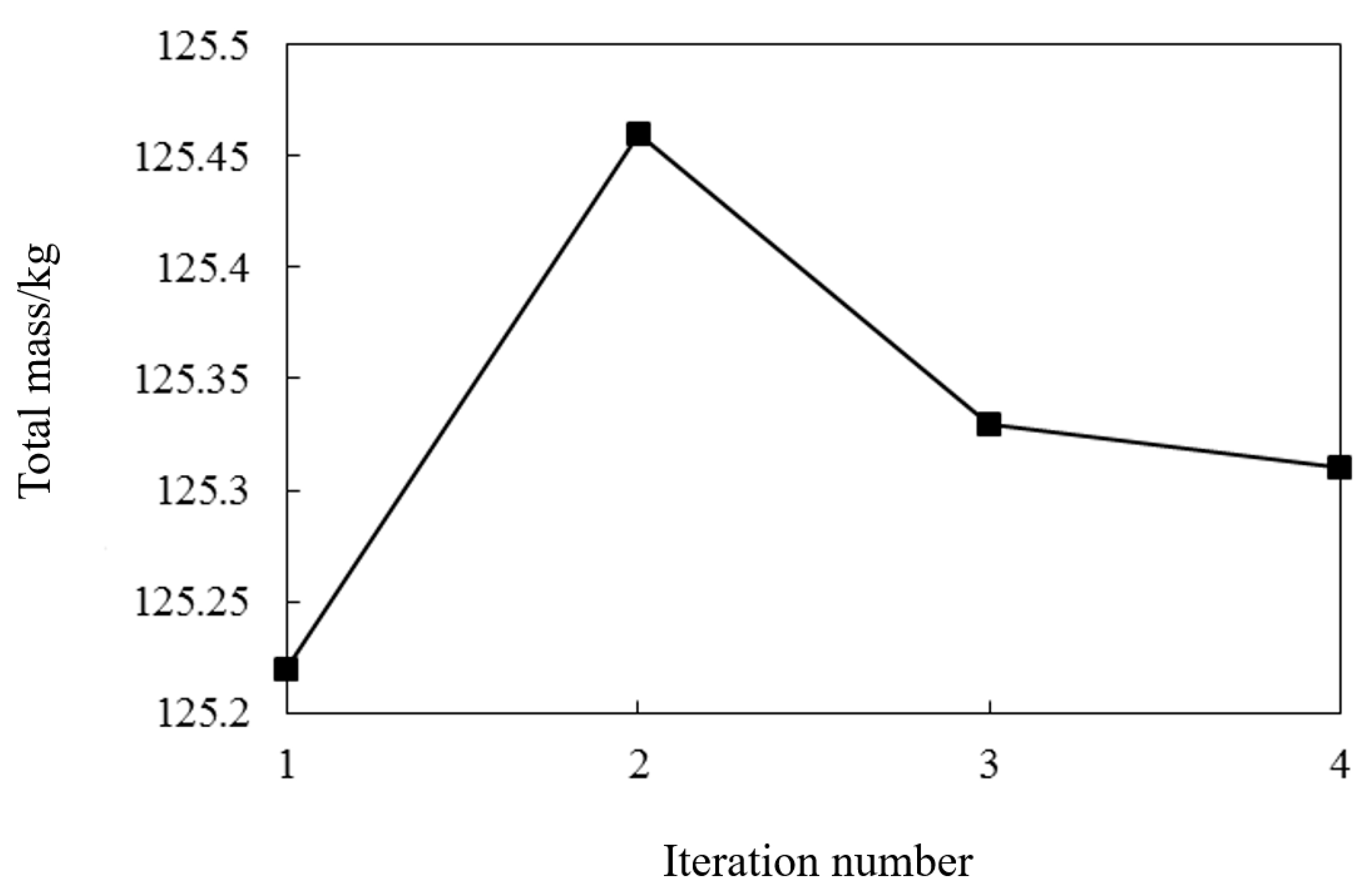
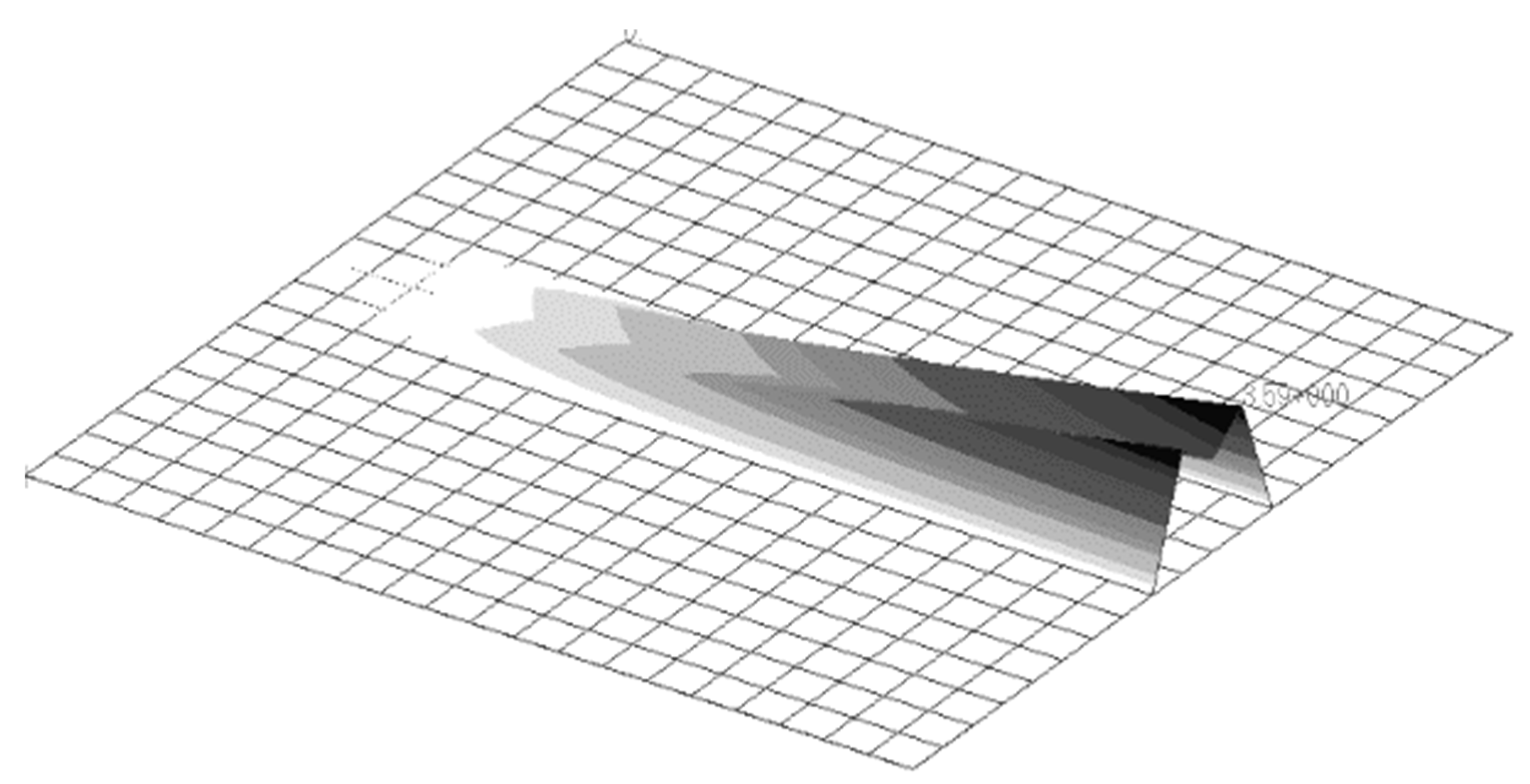
The optimization results are listed in Table 3. The iteration history is shown in Figure 7. The final structural weight increased by 0.09 kg compared with the initial weight, complying with the above Assumption 1. The maximum displacement from the static analysis was 0.359 m, satisfying displacement constraints condition of the approximate optimization model.
To verify the accuracy of the approximation method, we conducted a modal analysis of the plate with the present parameters, which resulted in the local modal shape shown in Figure 8, and the result of static analysis is shown in Figure 9. Approximate similarities of the initial and the present local modal shapes were found from Figure 8, which corresponded to the above Assumption 2. Upon further observation, the local frequency also met the design requirement and there was only a relative error of 1.29%.
In Reference [18], there was the same plate example of local frequency constraint, where the local mode identification technique was applied. The optimal weight was 125.29 kg while the local frequency was 60.003 Hz after five iterations. Compared to the previous result, with the transformation method, the optimal weight was 0.02 kg heavier and the local frequency was 0.7 Hz higher, which were close, but with fewer optimization iterations. That indicated the relative validity of this method.
5.2. Example 2: Satellite Structure
In this example, the proposed method was applied in a practical satellite composed of a service cabin and a payload cabin. Based on the original design, an FE model consisting of shell and beam elements was established. The boundary condition was to fix the bottom of the joint ring in view of the connecting interface between the launch vehicle and the satellite.
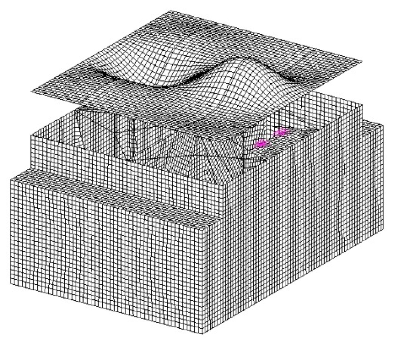
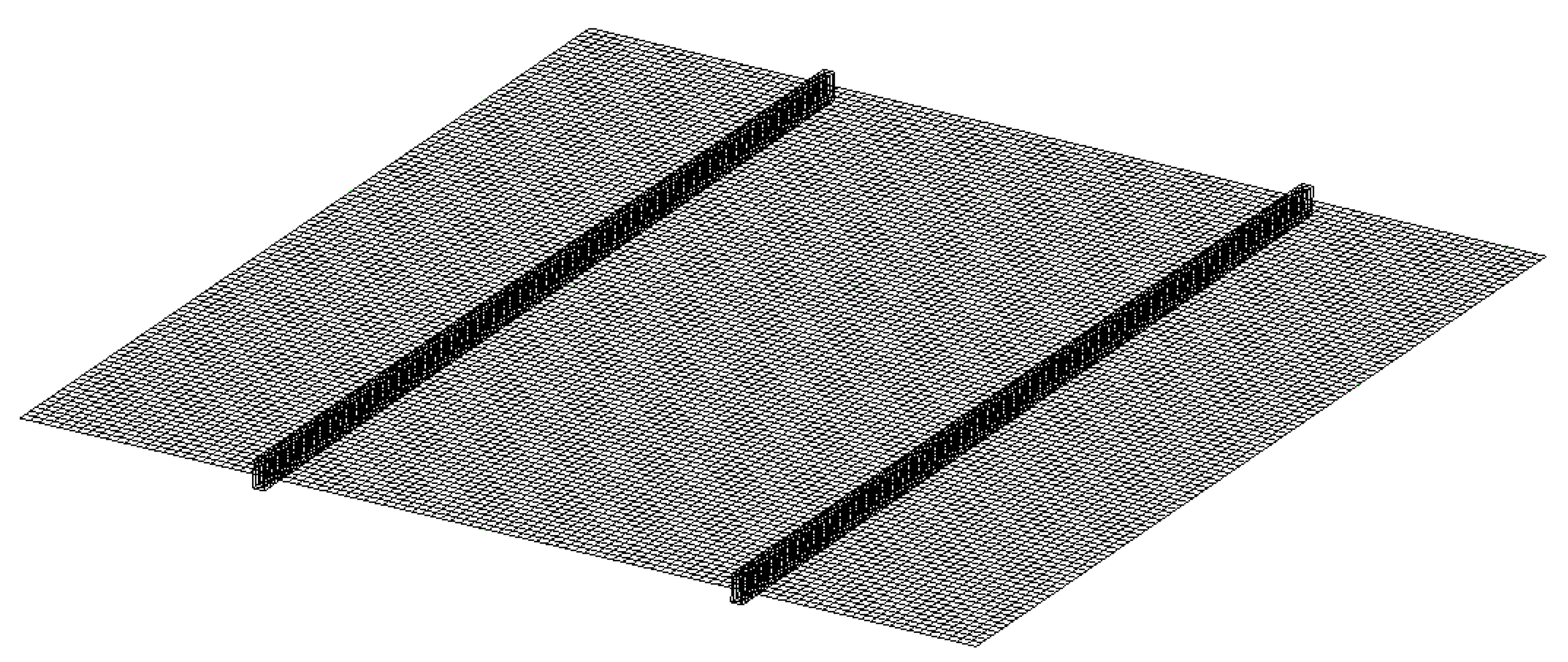
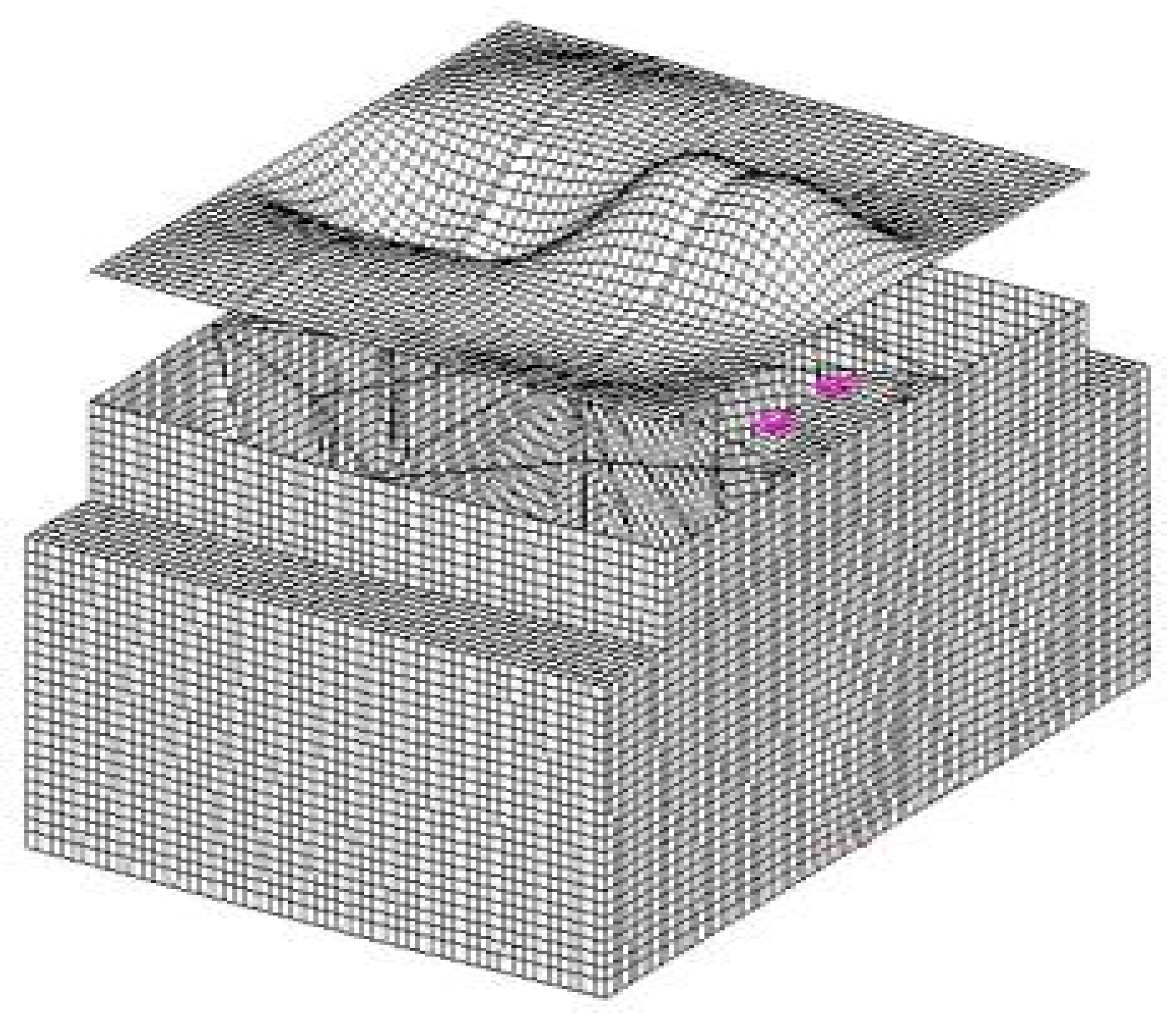
The modal analysis results indicated that there was a high vibration of densities on the horizontal plate of the satellite. Figure 10 shows the local modal shape of the horizontal plate. From this basis, the design domain was specified as the horizontal plate. Figure 11 shows where the stiffener was placed, influenced by the surrounding structures. Here, the minimum structural weight was to be found with the local frequency to be extended beyond 60 Hz to insulate it from the global frequency.
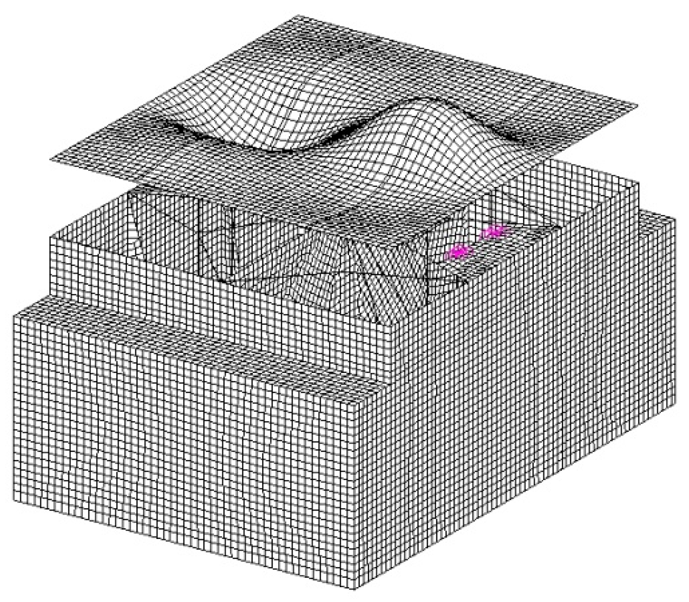
With the same techniques used in the previous example to apply the static load, the nodal displacements in the design domain were obtained. Displacements results of the satellite were shown in Figure 11.
The concordance between the displacements and the local modal shape could be seen directly from Figure 10 and Figure 12, thus, the approximate scalar finite element model could be developed.
A rectangular stiffener was placed where the maximum displacement occurred to increase the local frequency. In the approximate problem, the design variables were the cross-section dimensions of the stiffeners. The minimum structural weight was to be found. The initial design was H = W = 0.01 m; lower bounds of 0.001 m and upper bounds of 0.1 m were imposed on both design variables.
In the optimization problem, the local frequency was constrained to be at least 60 Hz, which is 1.43 times the initial. Therefore, in approximate optimization problem, nodal displacements on the reinforced stiffeners were constrained to be at most 0.029.
The whole optimization took four iterations to reach the optimal solution. In the last two iterations, there was not much change in the objective function. The optimization results are listed in Table 4.
The weight of stiffener accounted for 1.351% of the local plate weight and 0.043% of the initial total weight. The small percentage also reflected that the results were consistent with Assumption 1. The difference of the frequency order between the initial and optimized design indicated that the order change of local frequency was remarkable. Considering verifying the accuracy of our approximate model, an analysis for the local mode using the plate with the optimized parameters resulted in the modal shape shown in Figure 13. The displacements constraint and the frequency were both satisfied, and there was also a small relative error of 0.54%. Upon further observation of the optimized mode, approximate similarity of the optimized and initial modal shape was found, which corresponded to Assumption 2. This example verified the effectiveness of the proposed method in practical problem.
6. Conclusions
In this paper, the minimum weight optimization of structures with local frequency constraints has been addressed. Previous work has illustrated that the mode switching of local mode would cause convergence difficulties to the optimizer. An approximate method of transforming the local frequency constraint into displacements constraint without mode tracking is offered for dealing efficiently with this issue. The process mainly contains modal analysis of the initial design, the nodal equilibrium forces extraction, and optimization with nodal displacement constraint. With the proposed method, the mode identification can be avoided and the static analysis could reduce the computational cost.
The method presented here has been verified with two numerical examples. The first example of the stiffened plate examined the process of the approximation method and showed the reasonability of the three assumptions. The second example was a practical satellite application in which we intended to improve the local frequency of one piece of plate. The approximate method was shown to be very efficient in large practical structure with a small number of iterations. The optimization result indicated the feasibility of the proposed method.
Author Contributions
Conceptualization, J.L.; validation, Z.D.; formal analysis, Y.L.; writing—original draft preparation, Z.D.; writing—review and editing, S.C.; supervision, S.C.; project administration, S.C. and W.S.; funding acquisition, S.C. and W.S. All authors have read and agreed to the published version of the manuscript.
Funding
This work was funded by the National Natural Science Foundation of China; Grant Number: 11672016.
Conflicts of Interest
The authors declare no conflict of interest.
References
- Zhu, J.; Zhang, W.; Qiu, K. Local Modal Analysis of Structural Dynamic Topology Optimization. Chin. J. Aeronaut. 2005, 26, 619–623. [Google Scholar]
- Grandhi, R. Structural optimization with frequency constraints—A review. AIAA J. 1993, 31, 2296–2303. [Google Scholar] [CrossRef]
- Khan, M.R.; Willmert, K.D. An efficient optimality criterion method for natural frequency constrained structures. Comput. Struct. 1981, 14, 501–507. [Google Scholar] [CrossRef]
- Venkayya, V.B.; Tischler, V.A. Optimization of Structures with Frequency constraints. Am. Soc. Mech. Eng. 1983, 54, 239–259. [Google Scholar]
- Garrent, N. An Effective Approximation Technique for Frequency Constraints in Frame Optimization. Int. J. Numer. Methods Eng. 1988, 26, 1067–1069. [Google Scholar]
- Sigmund, O.; Bendsoe, M.P. Topology Optimization-Theory, Methods and Applications; Springer: Berlin, Germany, 2004. [Google Scholar]
- Du, J.; Olhoff, N. Topological design of freely vibrating continuum structures for maximum values of simple and multiple eigenfrequencies and frequency gaps. Struct. Multidiscip. Optim. 2007, 34, 91–110. [Google Scholar] [CrossRef]
- Yamada, S.; Kanno, Y. Relaxation approach to topology optimization of frame structure under frequency constraint. Struct. Multidiscip. Optim. 2016, 53, 731–744. [Google Scholar] [CrossRef]
- Li, Q.; Wu, Q.; Liu, J.; He, J.; Liu, S. Topology optimization of vibrating structures with frequency band constraints. Struct. Multidiscip. Optim. 2021, 63, 1203–1218. [Google Scholar] [CrossRef]
- Li, J.; Chen, S.; Huang, H. Topology optimization of continuum structure with dynamic constraints using mode identification. J. Mech. Sci. Technol. 2015, 29, 1407–1412. [Google Scholar] [CrossRef]
- She, J. Research on Dynamic Topology Optimization of Three Dimension Continuum Structures with Frequency Constraints; Beijing University of Technology: Beijing, China, 2012. [Google Scholar]
- Deaton, J.D.; Grandhi, R.V. A survey of structural and multidisciplinary continuum topology optimization. Struct. Multidiscip. Optim. 2013, 49, 1–38. [Google Scholar] [CrossRef]
- Chou, C.-M.; Pappa, R.S. Identification of Local Modes Using Modal Mass Distributions. In Proceedings of the International Modal Analysis Conference, Las Vegas, NV, USA, 30 January–2 February 1989; Volume 2, pp. 772–776. [Google Scholar]
- Tenek, L.H.; Hagiwara, I. Eigen-Frequency Maximization of Plates by Optimization of Topology Using Homogenization and Mathematical Programming. J. Mater. Sci. Mater. Electron. 1994, 37, 667–677. [Google Scholar]
- Pedersen, N.L. Maximization of Eigenvalues Using Topology Optimization. Struct. Multidiscip. Optim. 2000, 20, 2–11. [Google Scholar] [CrossRef]
- Cheng, G.D.; Wang, B. Constraint Continuity Analysis Approach to Structural Topology Optimization with Frequency Objective/Constraint. In Proceedings of the Seventh Word Congress on Structural and Multidisciplinary Optimization, Seoul, Korea, 21–25 May 2007. [Google Scholar]
- Xu, B.; Jiang, J.; Tong, W.; Wu, K. Topology group concept for truss topology optimization with frequency constraints. J. Sound Vib. 2003, 261, 911–925. [Google Scholar] [CrossRef]
- Chen, S.; Zheng, Y.; Liu, Y. Structural optimization with an automatic mode identification method for tracking the local vibration mode. Eng. Optim. 2018, 50, 1681–1694. [Google Scholar] [CrossRef]
Figure 1.
Optimization flowchart.

Figure 2.
FE model of the plate.

Figure 3.
The first four order mode shape of the initial model.

Figure 4.
FE model of the stiffened plate.

Figure 5.
The first four order mode shape of the model with the reinforced stiffener.

Figure 6.
The displacements result of the static analysis (Max dis = 4.12 m).

Figure 7.
Objective iteration curve.

Figure 8.
Local mode of the optimized model (local frequency = 60.77).

Figure 9.
Static nodal displacement of the optimized model.

Figure 10.
The local modal shape of the satellite.

Figure 11.
The arrangement of the stiffener.

Figure 12.
Displacement results of the satellite.

Figure 13.
The local modal shape of the optimal design (59.677 Hz).


Table 1.
Material property.
| Material | E | ||
|---|---|---|---|
| (white) | 200 × 109 N/m2 | 0.3 | 7800 kg/m3 |
| (black) | 200 × 103 N/m2 | 0.3 | 78 kg/m3 |
Table 2.
Design variables.
| Design Variables | Initial Design | Lower Bound | Upper Bound |
|---|---|---|---|
| H/m | 0.01 | 0.001 | 0.1 |
| W/m | 0.01 | 0.001 | 0.1 |
| t1/m | 0.002 | 0.001 | 0.1 |
| t2/m | 0.002 | 0.001 | 0.1 |
Table 3.
Optimization results for the thin plate example.
| Parameter | Initial Design | Optimized Design | |
|---|---|---|---|
| Design variables | H/m | 0.01 | 0.0436 |
| W/m | 0.01 | 0.0131 | |
| t1/m | 0.002 | 0.001164 | |
| t2/m | 0.002 | 0.0010 | |
| Maximum displacement/m | 4.12 | 0.359 | |
| Local frequency/Hz | 22.504 | 60.771 | |
| Order of the local frequency | 3 | 3 | |
| Total mass/kg | 125.22 | 125.31 | |
Table 4.
Optimization results for the satellite example.
| Parameter | Initial Design | Optimized Design | |
|---|---|---|---|
| Design variables | H/m | 0.01 | 0.0518 |
| W/m | 0.01 | 0.00258 | |
| Maximum displacement/m | 0.059 | 0.022 | |
| Local frequency/Hz | 42.234 | 59.677 | |
| Order of the local frequency | 36 | 71 | |
| Local plate mass/kg | 259 | 262.5 | |
| Total mass/kg | 8186 | 8189.5 | |
Publisher’s Note: MDPI stays neutral with regard to jurisdictional claims in published maps and institutional affiliations. |
© 2021 by the authors. Licensee MDPI, Basel, Switzerland. This article is an open access article distributed under the terms and conditions of the Creative Commons Attribution (CC BY) license (https://creativecommons.org/licenses/by/4.0/).
Share and Cite
MDPI and ACS Style
Chen, S.; Dai, Z.; Shi, W.; Liu, Y.; Li, J. Local Modal Frequency Improvement with Optimal Stiffener by Constraints Transformation Method. Appl. Sci. 2021, 11, 11072. https://0-doi-org.brum.beds.ac.uk/10.3390/app112211072
AMA Style
Chen S, Dai Z, Shi W, Liu Y, Li J. Local Modal Frequency Improvement with Optimal Stiffener by Constraints Transformation Method. Applied Sciences. 2021; 11(22):11072. https://0-doi-org.brum.beds.ac.uk/10.3390/app112211072
Chicago/Turabian StyleChen, Shenyan, Ziqi Dai, Wenjing Shi, Yanjie Liu, and Jianhongyu Li. 2021. "Local Modal Frequency Improvement with Optimal Stiffener by Constraints Transformation Method" Applied Sciences 11, no. 22: 11072. https://0-doi-org.brum.beds.ac.uk/10.3390/app112211072
Note that from the first issue of 2016, this journal uses article numbers instead of page numbers. See further details here.