
Estimating CPT Parameters at Unsampled Locations Based on Kriging Interpolation Method


1
Key Laboratory of Concrete and Prestressed Concrete Structures of Ministry of Education, Nanjing 211189, China
2
School of Civil Engineering, Southeast University, Nanjing 211189, China
3
Department of Statistics and Finance, School of Management, University of Science and Technology of China, Hefei 230026, China
*
Author to whom correspondence should be addressed.
Appl. Sci. 2021, 11(23), 11264; https://0-doi-org.brum.beds.ac.uk/10.3390/app112311264
Submission received: 7 October 2021
/
Revised: 7 November 2021
/
Accepted: 11 November 2021
/
Published: 29 November 2021
(This article belongs to the Special Issue Recent Progress on Advanced Foundation Engineering)
Abstract
:The cone penetrometer test (CPT) has been widely used in geotechnical investigations. However, how to use the limited CPT data to reasonably predict the soil parameters of the unsampled regions remains a challenge. In the present study, we adopted the Kriging method to obtain the CPT data of an unsampled location in Adelaide, South Australia, based on the collected CPT data from six soundings around this location. Interpolation results showed that the trend of the estimated parameters is consistent with the trend of parameters of the surrounding points. From the Kriging interpolation result, we further carried out axial bearing capacity calculation of a precast concrete pile using the CPT-based direct method to verify the reliability of the method. The calculated bearing capacity of the pile is 99.6 kN which is very close to the true value of 102.8 kN. Our results demonstrated the effectiveness of the Kriging method in considering the soil spatial variability and predicting soil parameters, which is quite suitable for the application in engineering practice.
1. Introduction
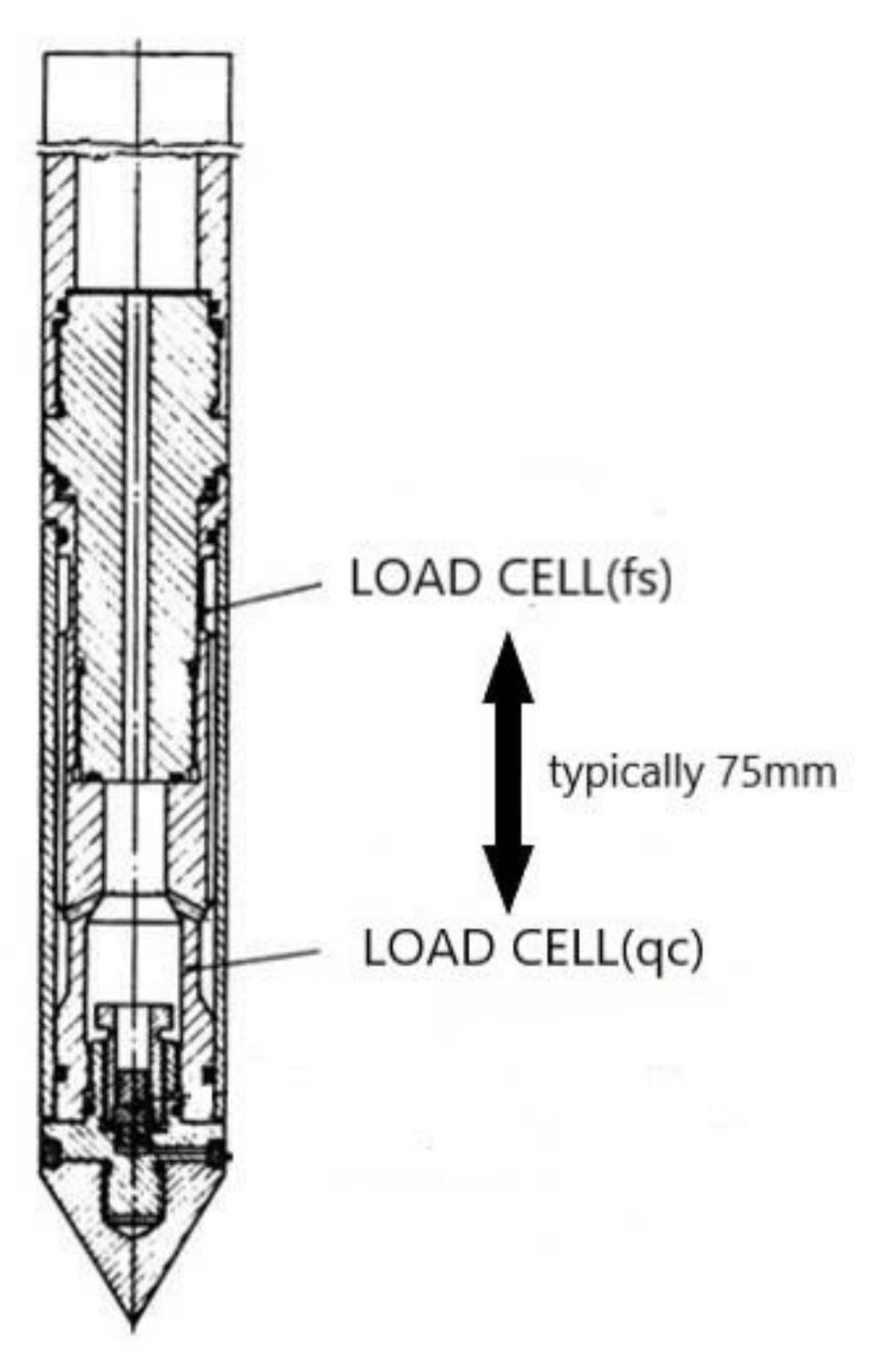
The cone penetration test (CPT) has been widely used as a quick and reliable soil exploration test that provides subsurface soil properties [1]. As the electric cone penetrometer (Figure 1) advances into the soil with a constant speed, parameters such as the cone tip resistance () and the sleeve friction () are simultaneously measured by the load cells on the penetrometer. Compared with other in situ tests, CPT can provide continuous parameter profiles that can yield much more detailed information [2]. As the two major measured parameters and vary significantly with the change of the soil layers, CPT shows advantages in geotechnical investigations to classify soil strata, and several methods have been proposed to classify soils upon CPT data [3,4,5]. Moreover, CPT can also be used to estimate the strength and deformation characteristics of soils, such as the undrained shear strength of soil [6]. Generally speaking, CPT is only conducted at necessary locations to obtain the required soil properties, for example, around the underground structure to be constructed. Considering the spatial variability of the soil, the CPT data obtained from adjacent soundings could be quite different, which makes it difficult to estimate the soil properties at the unsampled locations. Therefore, for large areas, how to reasonably estimate the soil properties of the entire area through limited CPT data is of great importance.
Soil properties are regionalized variables; that is, within a soil layer or rock mass, samples that are close to each other indicate a stronger correlation than distant ones [7]. Because CPT parameters directly depend on the soil properties, they are also autocorrelated. In statistics, there are two ways to consider the correlation of the data sequence with distance: one is random field theory, and the other is geostatistics. Random field theory is often used to analyze time series. Although it has been successfully applied in analyzing soil spatial variability by different researchers [8,9], it is mostly applied to one-dimensional situations.
Geostatistics often refers to the Kriging method, which has been widely used in the field of geographic science. Different from random field theory, the Kriging method can be applied to multi-dimensional analysis since it is an algorithm for spatial modeling and regression interpolation [10]. It has been used by many researchers to analyze the autocorrelation of geotechnical parameters and achieved promising results [11,12]. However, there are only a few case studies on adopting the Kriging method to predict the soil parameters at the unsampled locations, and the data used in previous studies is often scarce, which is not enough to prove the accuracy and effectiveness of the Kriging method. Currently, there have been several studies using Markov chain and machine learning methods combined with CPT test to predict the soil parameters at the unsampled locations [13,14]; however, they need to meet some strong prerequisites. For example, the Markov chain method is suitable when the unsampled location and the sampled CPT boreholes are located on the same horizontal line, while the machine learning method needs to obtain the soil layer information in advance and perform extensive training to obtain a better prediction result, which is difficult to be applied into practical engineering. In this study, we used CPT parameters with small sampling intervals as the research objects to assess the performance of the Kriging method in predicting spatial soil parameters, thus avoiding data insufficiency due to excessive sample spacing. The study was further supplemented by axial bearing capacity calculation, which we used to examine the reliability of the interpolation results and the applicability of the Kriging method in solving practical engineering problems.
2. Materials and Method
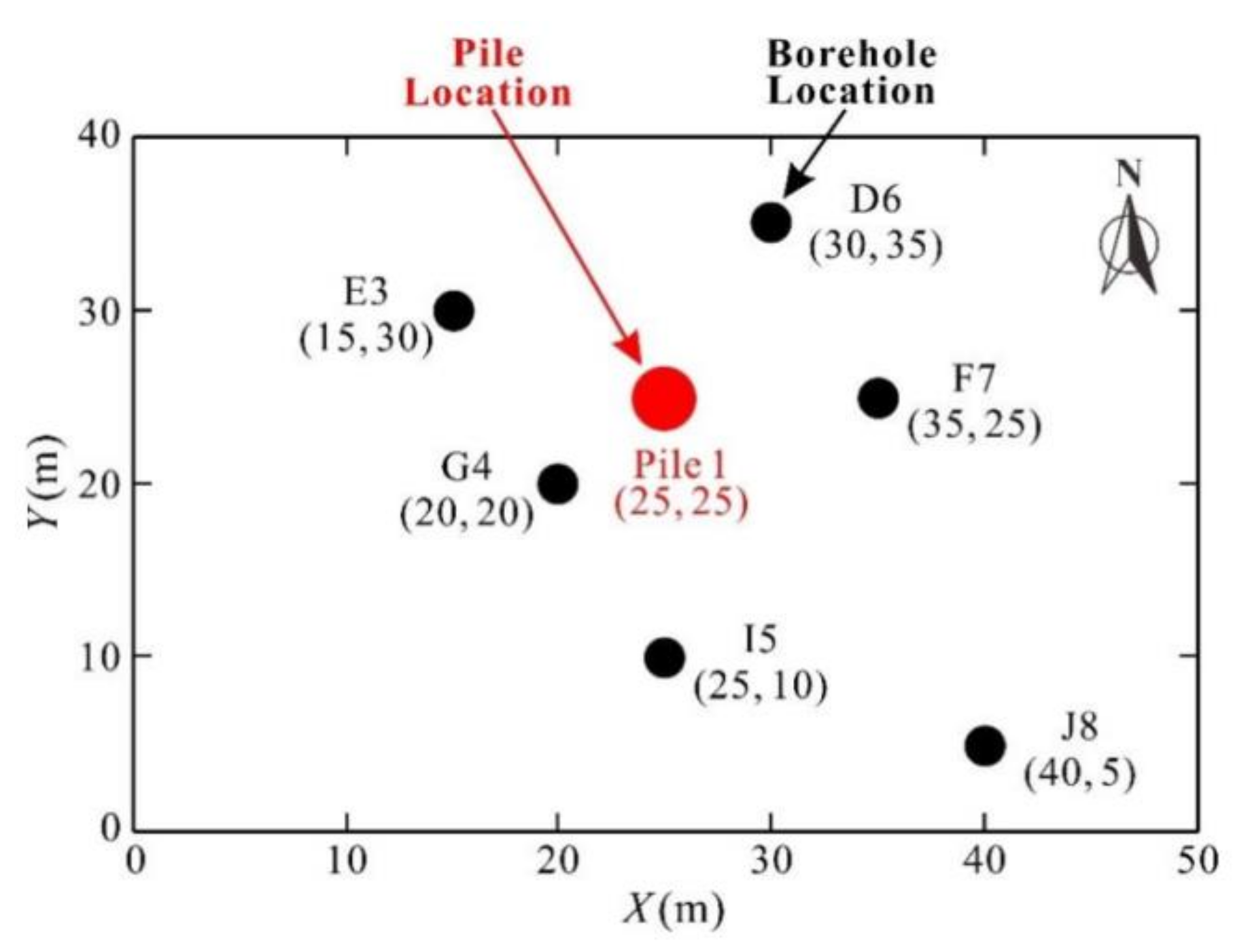
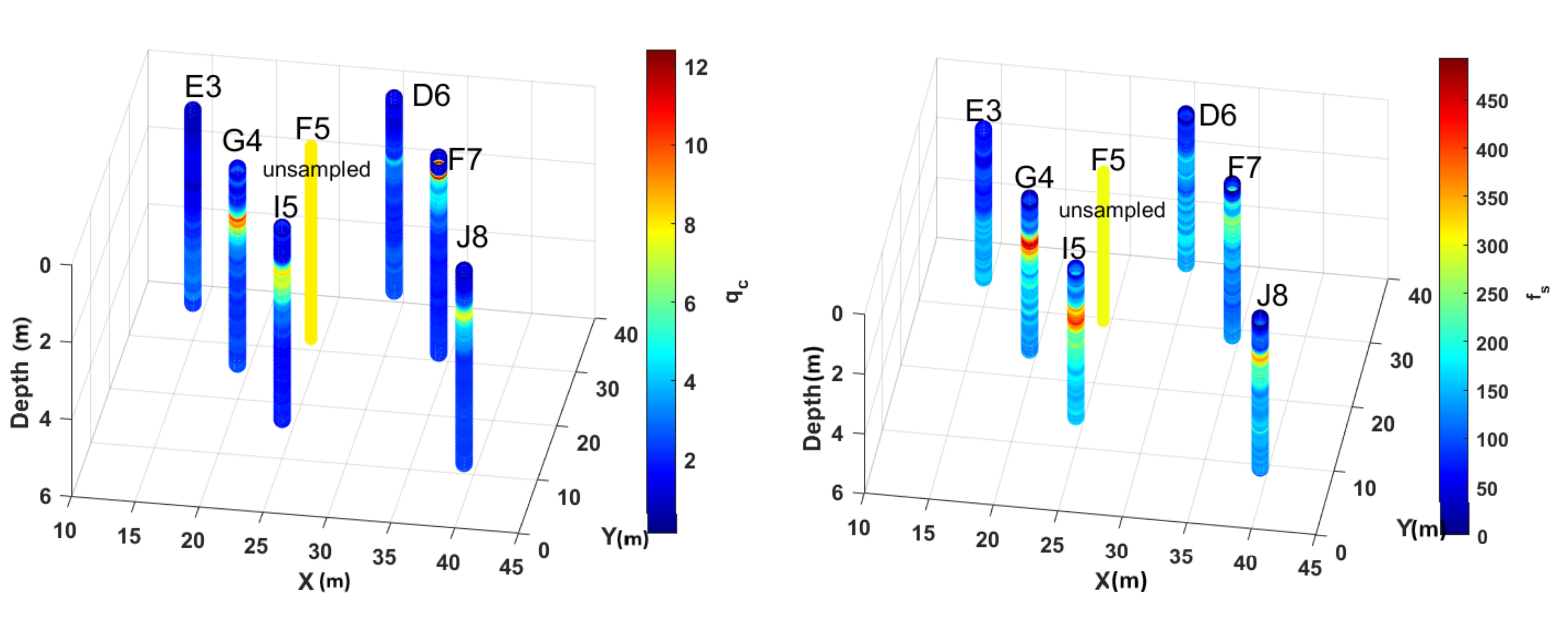
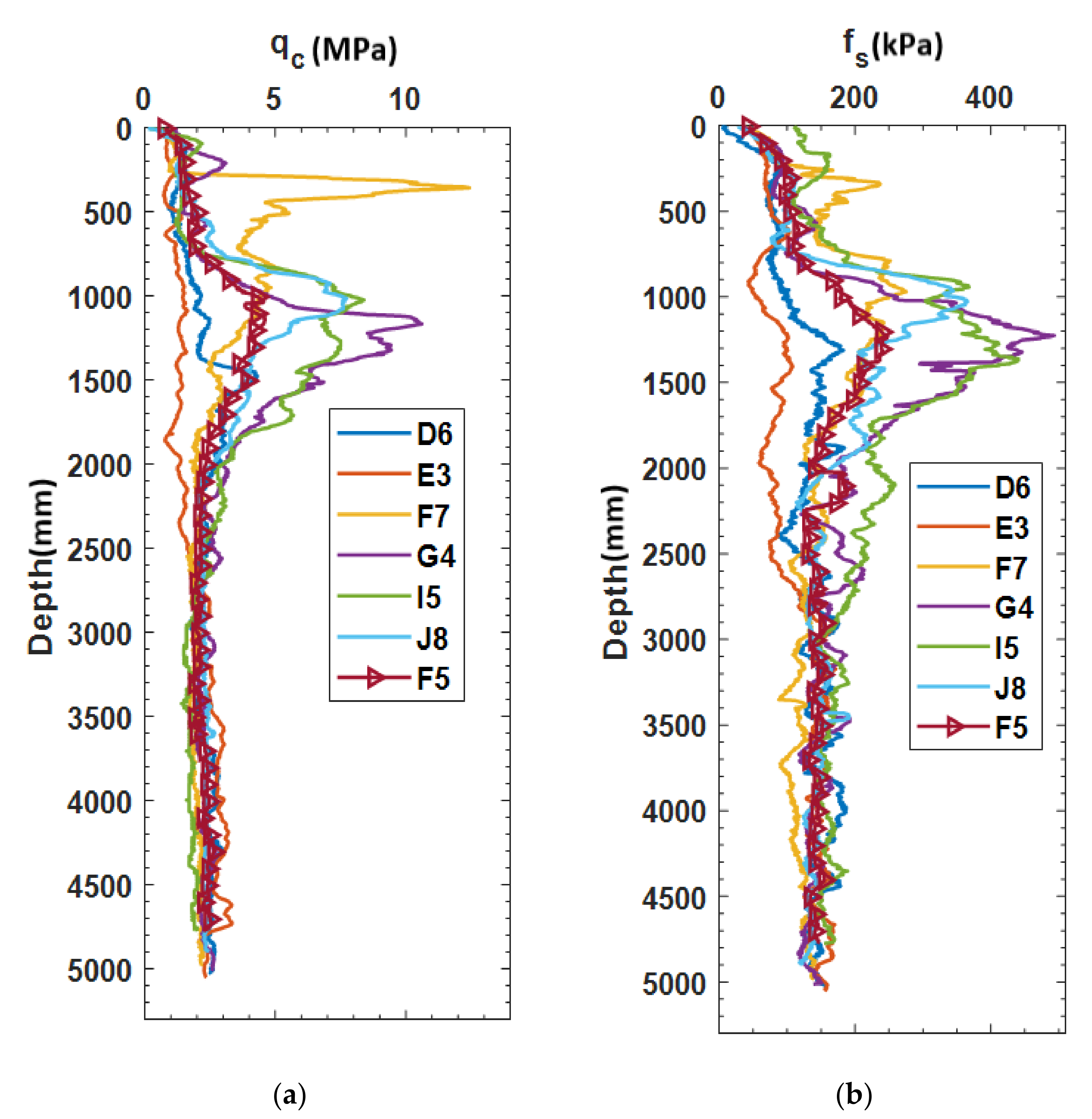
The CPT data is provided by the ISSMSG TC304 Student Contest Committee. As shown in Figure 2, there are six numbered CPT sampled boreholes randomly distributed on this 50 × 40 m field represented by the black points. The typical drilling depth is 5 m below the mud surface, and the measurement spacing is 5 mm (i.e., a total of 1000 and would be obtained for each borehole). Figure 3 shows the profiles of and values with depth at 6 sampled positions. A precast concrete pile was driven at an unsampled location shown by the red point numbered F5. In order to figure out the soil properties and evaluate the ultimate bearing capacity of this pile foundation, the Kriging method is adopted to interpret the and at the pile location based upon the available CPT data. However, the raw CPT data needs preprocessing before it can be used in the Kriging interpolation program.
CPT Data Preprocessing
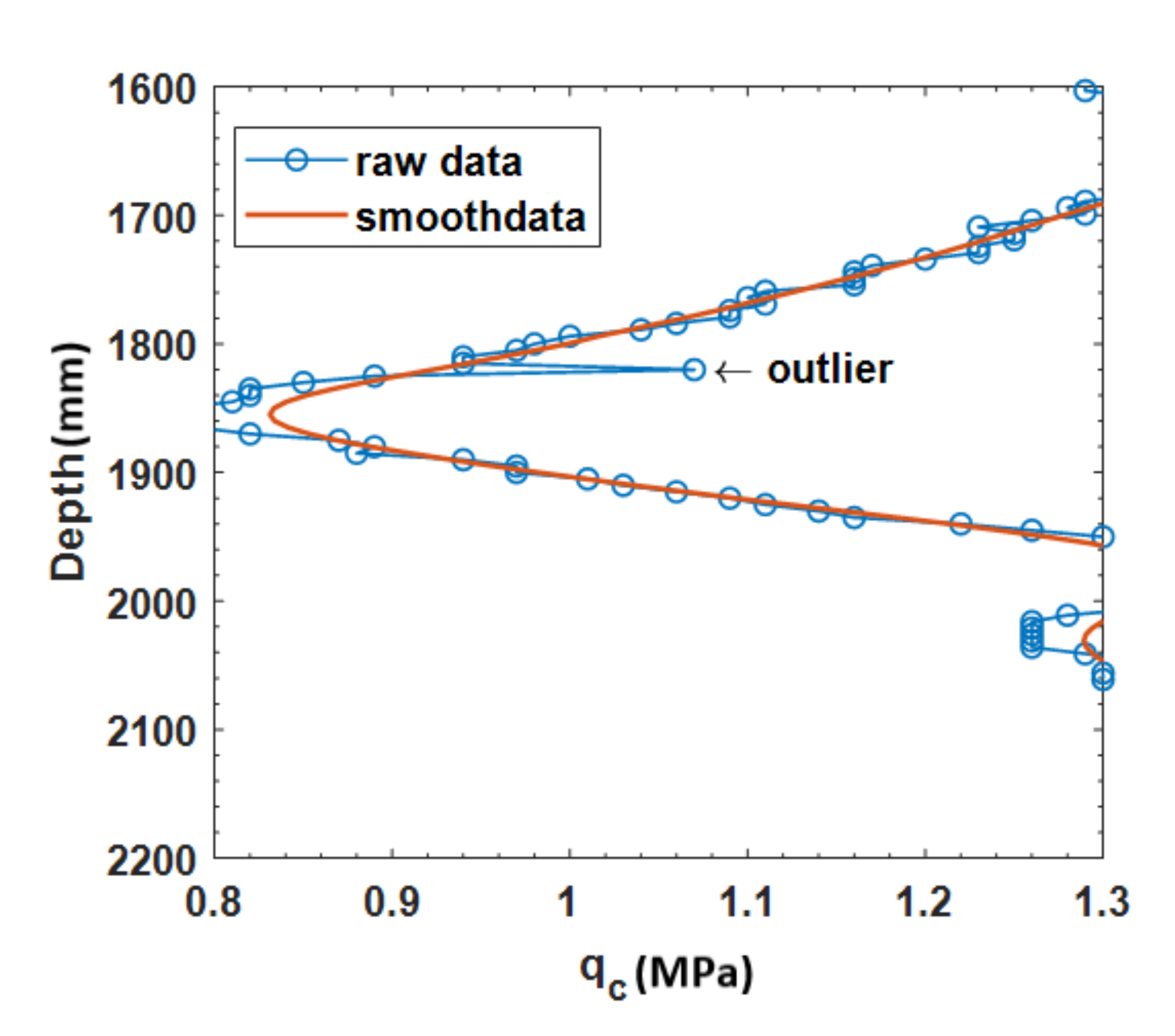
The first step is to remove outliers from the data. Outliers refer to those abnormal points whose values are obviously different from the surrounding sampled points, which is mainly caused by measurement errors or procedural errors such as rod adding [7]. Outliers do not reflect the actual CPT characteristics of the sampled points but affect the estimation accuracy, so they need to be removed first. This process is accomplished by a Gaussian filter, which replaces the value of the abnormal point with the weighted average of 20 samples around the point. The example of outliers and the smoothed curve is shown in Figure 4.
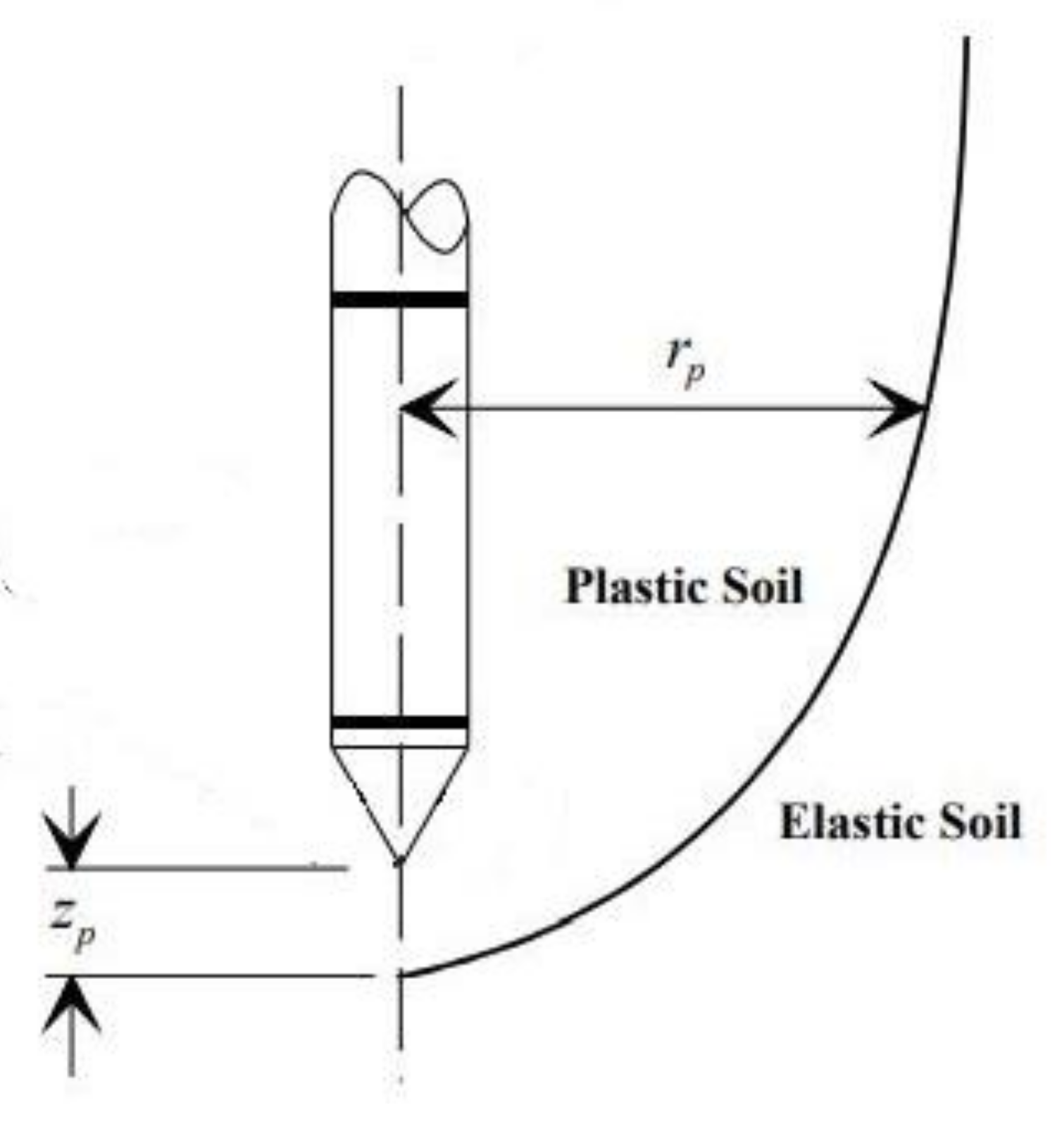
The second step is to shift the data to the right place. Schmertmann [15] emphasized that incorrect analysis will be made unless a depth correction, or shift, is applied to the measurements. This correction is required since the cone tip resistance, and sleeve friction load cells are physically separated by a given distance as shown in Figure 1, and hence measurements of do not refer to the same soil as that at which measurements of are taken. Schmertmann [15] recommended that this shift distance should be equal to the distance between the base of the cone and the mid-height of the sleeve, which, for standard electric cone penetrometers, is approximately 75 mm. Campanella et al. [16] argued that the shift distance, also termed the “friction-bearing offset”, is 100 mm and is dependent on the type of soil being penetrated. Actually, when the cone penetrometer is advanced into the subsoil, it will cause a zone of soil to fail and deform plastically, as shown in Figure 5. The and are not point values but spatially averaged values of the failure zone [17], and the shift distance would be different for different cases. Jaksa [7] recommended cross-correlation function (CCF) to determine the shift distance because of its superiority in demonstrating the cross-correlation between and .
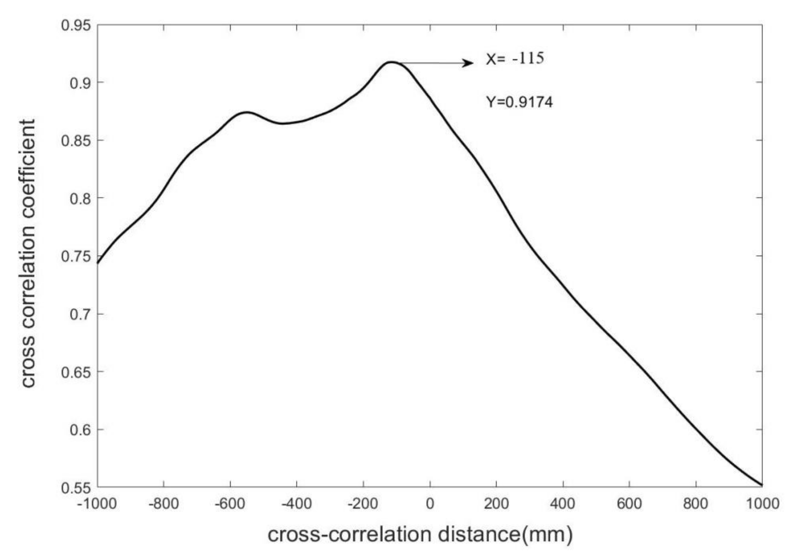
In this study, we adopted the CCF to determine the final shift distance. Taking the and data of borehole F7 as an example, the CCF analysis result is shown in Figure 6. It can be seen clearly from Figure 6 that the maximum cross-correlation coefficient occurs at a spacing of 115 mm, which implies that the optimal shift distance is 115 mm, which is higher than the actual physical spacing of 75 mm. The same process is applied to the other five boreholes, and the final shift distance results are shown in Table 1. Based on the result listed in Table 1, the data of the 6 boreholes will be shifted upward, resulting in a decrease in the maximum available drilling depth of each borehole. The smallest depth is borehole I5, of which the available depth of is reduced to 4775 mm so that in the interpolation part, the maximum interpolation depth is adjusted to 4775 mm. Meanwhile, in order to solve the problem of missing data at some depth in some boreholes, we use linear interpolation to fill in the missing values, and the details are shown in Appendix A.
After the above preprocessing steps, we divided the soil into a total of 956 sections from the ground down every 5 mm until the depth of 4775 mm, then on each section, we estimated the CPT parameter at the unsampled location using the Kriging method.
3. Kriging Interpolation
3.1. Set Up Semivariogram
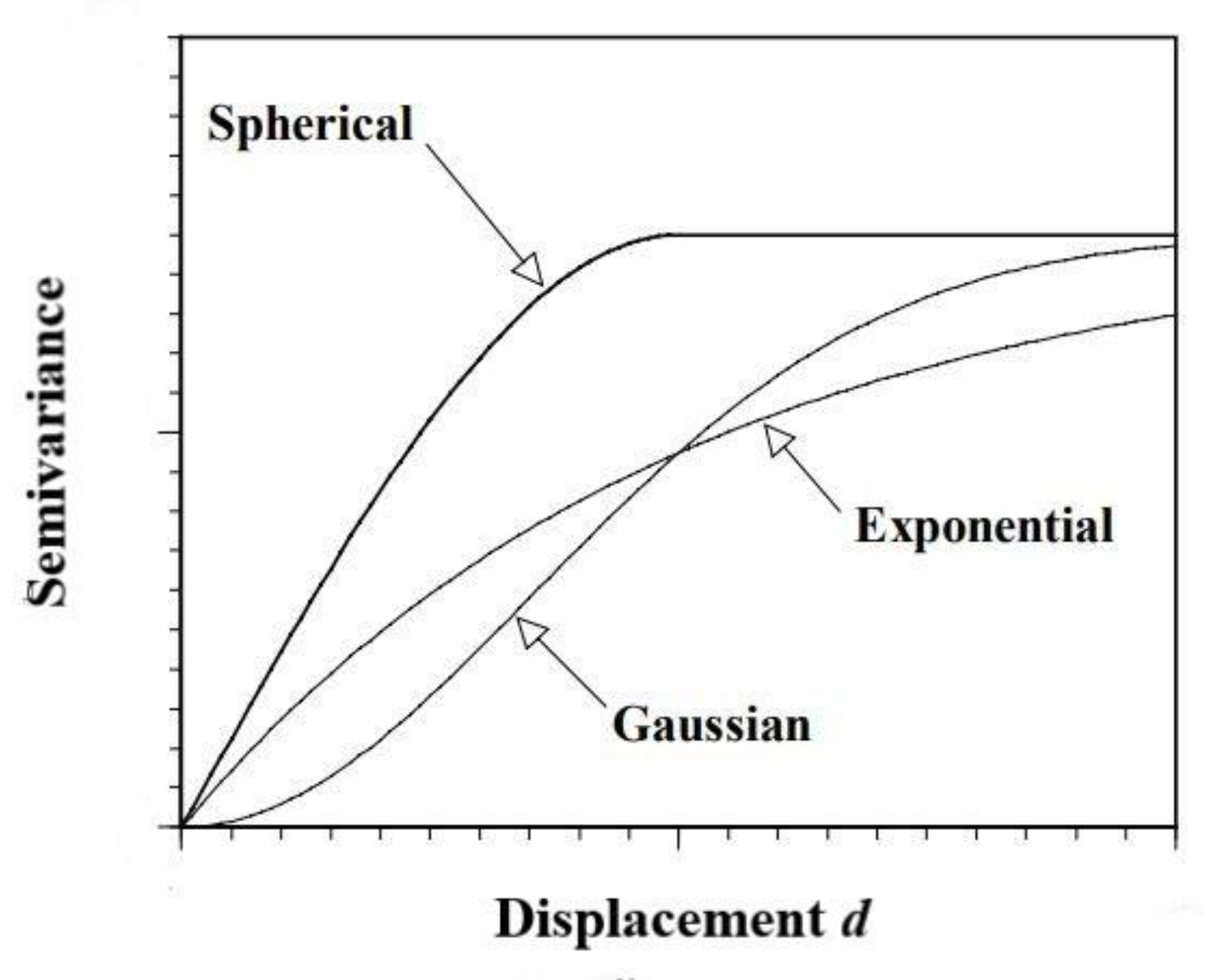
The core theory of the Kriging method is the semivariogram, which is established to reflect the relationship between distance and semivariance between two sampled points. Generally speaking, the semivariogram is an increasing function. The larger the semivariance, the smaller the spatial dependence and mutual influence between the two sample points. According to the different forms of the semivariogram, different models are selected for fitting. Figure 7 shows some commonly used semivariogram models in the literature, such as the spherical model, exponential model, and Gaussian model. Soulié [18] used semivariogram to analyze the spatial variability of CPT data performed in alluvial deposits of sand and gravel in the Mississippi River flood plain, and the results showed that the spherical model was more proper for fitting the actual curve compared with other models. In addition, previous studies also demonstrated that the spherical model can fit well to the semivariogram of various soils [19]. So in this study, we also chose a spherical model to fit the semivariogram.
The semivariogram is defined as follows:
where: is the variable at location, x;
is the variable at location, x + d;
d is the distance between the sample pairs;
Var[x] refers to the variance of x.
Equation (1) implies that the nature of the semivariogram function is half the variance of and , sample pairs separated by d, and for a certain semivariogram, the variance is dependent only on d. This hypothesis, however, is hard to be satisfied for soil, for example, , , and are samples at different depths in the same CPT borehole, and the distance from x2 to x1 and x3 is the same. The hypothesis means that x2 should have the same effect on the other two points, but if x2 and x1 are in the same layer and x3 is in another layer, then x2 will obviously have different effects on the other two points. Although the hypothesis is difficult to meet, the Kriging interpolation is still a reasonable estimation method under the condition that the information of the soil layer at the estimation point is unknown.
The variables used to plot the semivariogram should satisfy the following equation:
where E[x] refers to the expectation of x.
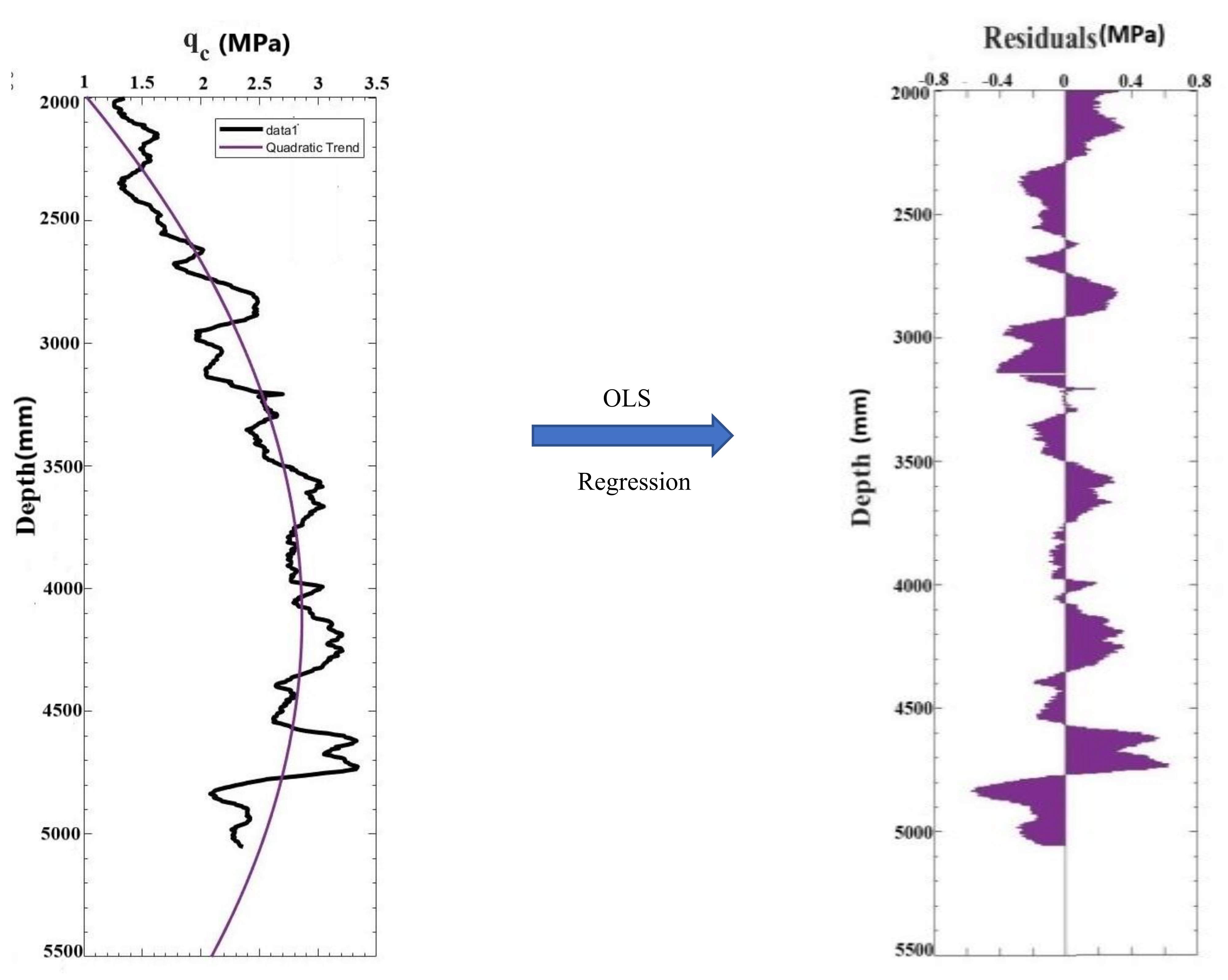
As shown in the above equation, all the variables within the study area should have the same expectations, which are always called stationary variables. Figure 8 shows the profiles of borehole E3, and it is clear from Figure 8 that CPT data are not stationary but with a specific trend. In order to satisfy Equation (2), ordinary least squares regression is performed to estimate the trend. After that, the trend component will be removed from the original CPT data so that the residuals would be stationary, and the semivariogram could be established upon it. The process is shown in Figure 8.
Considering Equation (2), Equation (1) can be simplified as:
In practice, the semivariogram must be estimated from the available discrete data, i.e., the theoretical expectations could be estimated by sample mean:
where N is the number of point pairs that are separated by distance d.
3.2. Build Weight Matrix
After the determination of the semivariogram based on existing data, it is feasible to estimate the CPT parameters at the unsampled location. Specifically, the Kriging method assigns different weights to the sampled CPT parameters at different locations, then linearly combines these parameters with their weights to obtain the estimation as shown by Equations (5) and (6). Where e indexes the unsampled location, i indexes the ith sampled location, Z is the CPT parameter (i.e., or ), is the corresponding weight, and is the number of samples. The weight could be obtained by solving marix presented in Equations (7) and (8).
where is Lagrange constant and is the value of semivariogram corresponding to distance between th and th location. The Kriging method is unbiased implying that the expectation of the estimator obtained from the above equations is equal to the actual value (i.e., the average of the estimation errors will be zero). The final and profiles of the target location F5 obtained by the Kriging method are shown in Figure 9, accompanied by data from the other six sampled boreholes. The detailed program implementation using MATLAB is shown in Appendix A.
4. Bearing Capacity Calculation
In order to examine the reliability of the Kriging interpolation results and its applicability to solve practical engineering problems, we use the interpolated CPT data of F5 to calculate the bearing capacity of a driven procast pile. The length and diameter of the pile are 4.5 and 0.3 m, respectively.
Based on previous studies, researchers held the point that the cone penetrometer can be considered as a mini-pile foundation, whereby the measured tip resistance () and sleeve resistance () correspond to the pile end bearing () and the component of side friction (). So far, many CPT-based axial bearing capacity calculation methods of pile foundation have been proposed [20]. Cai et al. [21] evaluated and graded 10 CPT-based methods by comparing the measured capacity from static load tests with the estimated result from different pile capacity prediction methods, and the results showed that the CPT-based methods had reliability and the Laboratoire Central des Ponts et Chausees method (LCPC, Bustamante and Gianeselli) [22] is one of the most accurate prediction methods. Another research conducted by Abu-Farsakh and Titi [1] obtained the same result that the LCPC method was relatively better when applied to predict the ultimate bearing capacity of square precast prestressed concrete (PPC) piles driven into Louisiana soils. Moreover, Jaksa [7] also recommended LCPC methods as the best prediction method for the soil in Adelaide.
For the LCPC method, the unit tip bearing capacity of the pile () is predicted from the following equation:
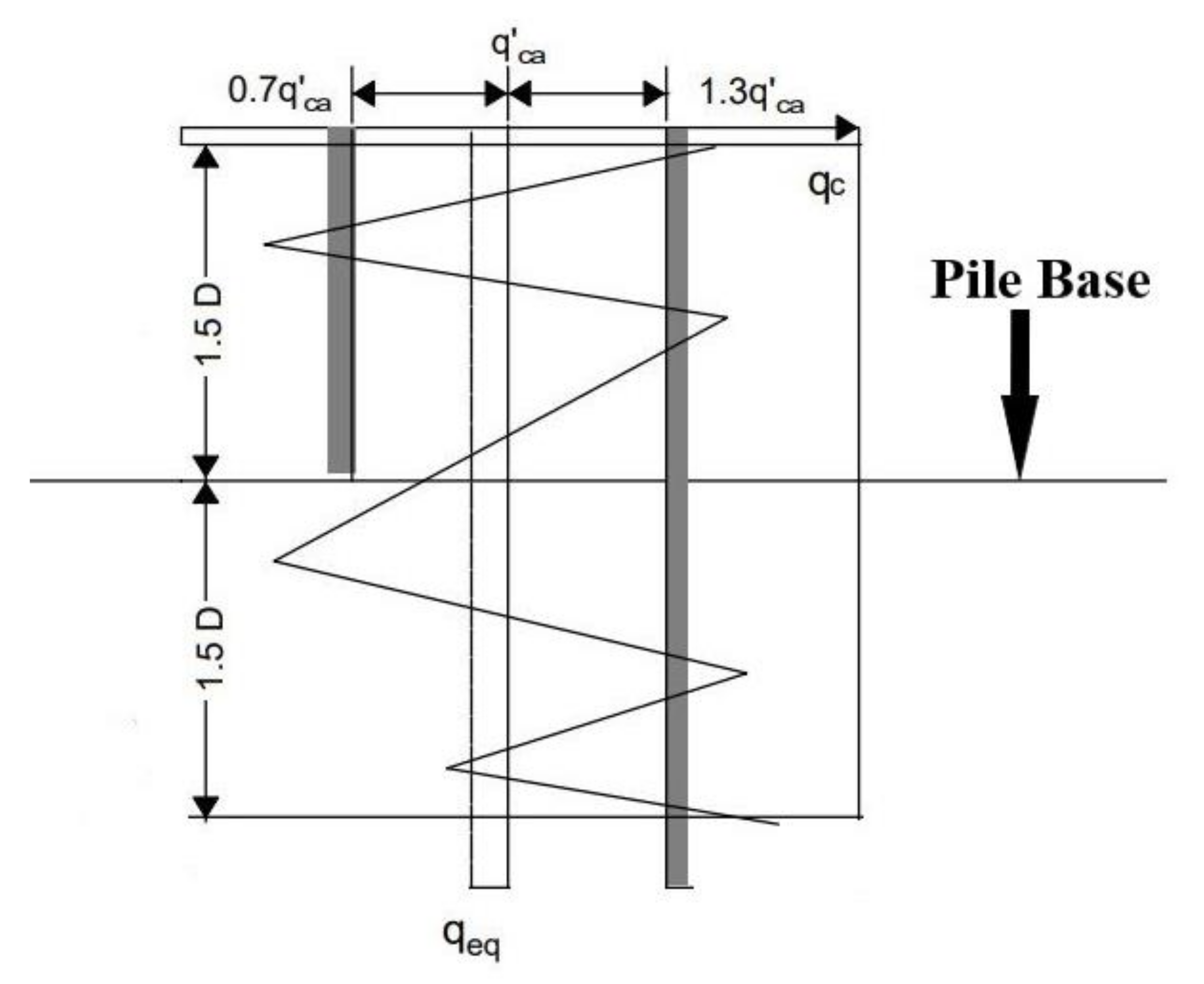
where kb = 0.45 for driven precast piles in clay or silt with values ranging from 1 to 5 MPa, is equivalent average cone tip resistance from 1.5 D above the pile tip to 1.5 D below the pile tip as shown in Figure 10.
Firstly, the average value in the upper and lower 1.5 D range is determined. Then the values higher than 1.3 or lower than 0.7 are eliminated. After that, the could be obtained by averaging the remained values over the same zone. In this study, due to data insufficiency and stability of values around the pile tip, as shown in Figure 9, is determined by averaging the values from 1.5 D above the pile tip to the last available value, and the result of is 1.089 MPa. Now the end bearing capacity can be determined as:
where: Ab is the end area of the pile, and the calculation result is 77 kN.
The pile unit skin friction is estimated by:
where ks is the skin friction coefficient ranging from 30 to 150 and equals 40 for driven procast piles in moderately compact clay ( range: 1 MPa–5 MPa). Bustamante and Gianeselli [22] also imposed different upper limits for depending on pile and soil typology as well as installation methods. In this case, the upper limit is 35 kPa. According to Equation (11), the data is first transformed to , and the data over 35 kPa is replaced with 35 kPa, then the data is used to calculate the total pile skin friction by Equation (12).
where is the side area of the ith layer, and the Qs is calculated to be 148 kN. Finally, Bustamante and Gianeselli [20] suggested that the allowable design load of the pile is defined by the following equation:
Through Equation (13), the final allowable design load is 99.6 kN. Jaksa [7] calculated the axial bearing capacity of the pile under the same condition through a 3D finite element model, of which the soil parameters came from the laboratory test on soil samples of the study area. The result given by Jaksa [7] is 102.8 kN, which is very close to our result.
5. Discussion
The Kriging method treats soil parameters as regionalized variables and considers the mutual influence by assigning different weights according to the semivariogram. In this study, we use the Kriging method combined with CPT data to make a reasonable estimation of the soil parameters at unsampled locations. Since CPT data is continuous and sufficient, our method can estimate parameters of locations within a certain scope and overcome the data insufficiency problem caused by relatively large sample spacings of the previous studies. As shown in Figure 9, line roughly reflects a similar trend as the other six sampled lines, with a fluctuation between depth 700–2000 mm for both and , and the data tends to keep stable under 2.5 m. The bearing capacity analysis further proved the effectiveness of the Kriging method.However, there are also some limitations for this study: The Kriging method relies on semivariograms, which need to be figured out on parameters at sampled locations. However, the number of available CPT soundings is limited, leading to instability of the result. For each cross-section, we only used six known and to set up the experimental semivariogram, which could not be quite accurate. More CPT tests are required for a better estimation. Due to the shift of , the maximum interpolation depth is 4775 mm, which cannot meet the requirement of calculating depth of the LCPC methods, so the calculation may have errors. What is more, the LCPC method poses an upper limit for , which may cause underestimation of the total bearing capacity, and the influence distance above and below the pile tip used in calculation is different for different methods [20]. Cai et al. [21] suggested that the influence distance given by the original method may be improper, and further study is needed to revise it depending on the soil type.
6. Conclusions
In summary, our research demonstrates the feasibility of using the Kriging method to consider the spatial variability of soil and provides a reliable estimation of soil parameters. Kriging methods can be combined with in situ tests and further applied into both geotechnical investigation and the analysis of the underground structures such as piles, bringing new directions and broad prospects in solving practical engineering problems.
Author Contributions
J.L. (Jinhao Liu): Material and Method, Writing—original draft. J.L. (Jinming Liu): Conceptualization, Writing—review and editing. Z.L.: Kriging interpolation, Program implementation. X.H.: Bearing capacity calculation. G.D.: Review and editing, Validation. All authors have read and agreed to the published version of the manuscript.
Funding
This research was funded by the National Natural Science Foundation of China (No.51878160, 52078128, 52008100).
Institutional Review Board Statement
Not applicable.
Informed Consent Statement
Not applicable.
Data Availability Statement
The collected CPT data are provided by ISSMSG TC304 Student Contest Committee, which can be downloaded at any time from publicly available datasets A-CPT/232/2500m2 dataset (Jaksa1995) in the 304 dB webpage (http://140.112.12.21/issmge/tc304.htm?=6) (Accessed on 10 November 2021).
Acknowledgments
The authors would like to express appreciation to the editors and reviewers for their valuable comments and suggestions. Guo-liang Dai is greatly appreciated for his useful suggestions, which have led to a substantial improvement of this paper. The study presented herein is supported by the National Natural Science Foundation of China (Nos. 51878160; 52078128; 52008100), Natural Science Foundation of Jiangsu Province (No. BK20200400). The authors are grateful for their support.
Conflicts of Interest
The authors declare no conflict of interest. The funders had no role in the design of the study, in the collection, analyses, or interpretation of data, in the writing of the manuscript, or in the decision to publish the results.
Appendix A
Linear interpolation program code using MATLAB
The same process is applied to the other five numbered boreholes to divide the soil into slices.
Kriging method program code
This paper uses the DACE toolbox developed based on MATLAB to complete the Kriging interpolation estimation of CPT data. Lophaven et al. (2002) established this toolbox to easily estimate the values of unsampled variables based on sampled data. This toolbox consists of two main functions for building the Kriging interpolation model and using the model to estimate the values of unsampled variables. The program code is as follows:
The description of each item in codes (A1) and (A2) is listed in Table A1. The code (A1) is used to build the model, which is used by the code (A2) to predict the result. As stated before, regpoly2 was used as a regression model to remove the quadratic trend of qc and fs, and corrspherical, that is, the spherical model was adopted to fit the semivariogram.

Table A1.
Description of code (8).
| Name | Description | Options |
|---|---|---|
| Location of sampled CPT borehole | ||
| Value of sampled CPT borehole | ||
| Regression model | * regpoly0, regpoly2 and regpoly3 | |
| Correlation model | * correxp, correpg, corrgauss, corrlin, corrspherical and corrspline | |
| Initial guess of correlation parameter | defaut | |
| Lower limit of correlation parameter | defaut | |
| Upper limit of correlation parameter | defaut | |
| DACE model | ||
x | Information about the optimization location of unsampled point |
* Note: regpoly0, regpoly2, and regpoly3 mean zero-order polynomial, first polynomial, and second-order polynomial; correxp, correpg, corrgauss, corrlin, corrspherical, and corrspline mean exponential model, generalized exponential model, Gaussian model, linear model, spherical model, and cubic spline model.
References
- Abu-Farsakh, M.Y.; Titi, H.H. Assessment of direct cone penetration test methods for predicting the ultimate capacity of friction driven piles. J. Geotech. Geoenviron. Eng. 2004, 130, 935–944. [Google Scholar] [CrossRef]
- Alex, S. Evaluation and Development of CPT Based Pile Design in Nebraska Soils. Civ. Eng. Theses Diss. Stud. Res. 2018, 127. [Google Scholar]
- Robertson, P.K. Soil classification using the cone penetration test. Can. Geotech. J. 1990, 27, 151–158. [Google Scholar] [CrossRef]
- Robertson, P.K.; Campanella, R.G.; Gillespie, D.; Greig, J. Use of piezometer cone data. In Use of In Situ Tests in Geotechnical Engineering; ASCE: New York, NY, USA, 1986; pp. 1263–1280. [Google Scholar]
- Eslami, A.; Fellenius, B.H. Pile capacity by direct CPT and CPTU methods applied to 102 case histories. Can. Geotech. J. 1997, 34, 886–904. [Google Scholar] [CrossRef]
- Jamiolkowski, M.; Presti, D.L.; Manassero, M. Evaluation of Relative Density and Shear Strength of Sands from CPT and DMT. In Symposium on Soil Behavior & Soft Ground Construction Honoring Charles C; Chunk Ladd: Cambridge, MA, USA, 2003. [Google Scholar]
- Jaksa, M.B. The Influence of Spatial Variability on the Geotechnical Design Properties of a Stiff, Overconsolidated Clay. Ph.D. Thesis, University of Adelaide, 1995. [Google Scholar]
- Liu, Y.; Li, J.; Sun, S.; Yu, B. Advances in Gaussian random field generation: A review. Comput. Geosci. 2019, 23, 1011–1047. [Google Scholar] [CrossRef]
- Lloret-Cabot, M.; Hicks, M.A.; van den Eijnden, A.P. Investigation of the reduction in uncertainty due to soil variability when conditioning a random field using kriging. Géotech. Lett. 2012, 2, 123–127. [Google Scholar] [CrossRef] [Green Version]
- Le, N.D.; Zidek, J.V. Statistical Analysis of Environmental Space-Time Processes; Springer Science & Business Media: Berlin/Heidelberg, Germany, 2006; pp. 101–134. [Google Scholar]
- Brooker, P.I.; Winchester, J.P.; Adams, A.C. A geostatistical study of soil data from an irrigated vineyard near Waikerie, South Australia. Environ. Int. 1995, 21, 699–704. [Google Scholar] [CrossRef]
- Chiasson, P.; Lafleur, J.; Soulié, M.; Law, K.T. Characterizing spatial variability of a clay by geostatistics. Can. Geotech. J. 1995, 32, 1–10. [Google Scholar] [CrossRef]
- Zhao, T.; Xu, L.; Wang, Y. Fast non-parametric simulation of 2D multi-layer cone penetration test (CPT) data without pre-stratification using Markov Chain Monte Carlo simulation. Eng. Geol. 2020, 273, 105670. [Google Scholar] [CrossRef]
- Zhao, T.; Wang, Y. Interpolation and stratification of multilayer soil property profile from sparse measurements using machine learning methods. Eng. Geol. 2020, 265, 105430. [Google Scholar] [CrossRef]
- Schmertmann, J.H. Guidelines for Cone Penetration Test, Performance and Design; Rep. No. FHWA-TS-78-209; U.S. Department of Transportation: Washington, DC, USA, 1978; p. 145. [Google Scholar]
- Campanella, R.G.; Robertson, P.K.; Gillespie, D. Cone penetration testing in deltaic soils. Can. Geotech. J. 2011, 20, 23–35. [Google Scholar] [CrossRef]
- Teh, C.I.; Houlsby, G.T. An analytical study of the cone penetration test in clay. Geotechnique 2015, 41, 17–34. [Google Scholar] [CrossRef]
- Soulié, M. Geostatistical Applications in Geotechnics. In Geostatistics for Natural Resources Characterization; Part 2; Springer: Berlin/Heidelberg, Germany, 1984; pp. 703–730. [Google Scholar]
- Soulié, M.; Montes, P.; Silvestri, V. Modelling spatial variability of soil parameters. Can. Geotech. J. 1990, 27, 617–630. [Google Scholar] [CrossRef]
- Niazi, F.S.; Mayne, P.W. Cone Penetration Test Based Direct Methods for Evaluating Static Axial Capacity of Single Piles. Geotech. Geol. Eng. 2013, 31, 979–1009. [Google Scholar] [CrossRef]
- Cai, G.; Liu, S.; Puppala, A.J. Reliability assessment of CPTU-based pile capacity predictions in soft clay deposits. Eng. Geol. 2012, 141–142, 84–91. [Google Scholar] [CrossRef]
- Bustamante, M.; Gianeselli, L. Pile Bearing Capacity Predictions by Means of Static Penetrometer CPT. In Proceedings of the Second European Symposium on Penetration Testing, ESOPT-II, Amsterdam, The Netherlands, 24–27 May 1982; Volume 2, pp. 493–500. [Google Scholar]
Figure 1.
Cone penetrometer of CPT.

Figure 2.
The locations of the sampled CPT boreholes and the pile.

Figure 3.
The qc and fs profiles of the six CPT soundings.

Figure 4.
Outlier of raw CPT data.

Figure 5.
Plastic failure zone caused by the cone penetrometer.

Figure 6.
CCF of borehole F7.

Figure 7.
Commonly used semivariogram models.

Figure 8.
Example of the CPT data detrend.

Figure 9.
The 2D and 3D Kriging interpolation results of the unsampled location F5: (a) 2D; (b) 3D.

Figure 10.
Calculation of the equivalent average tip resistance for the LCPC method.

Table 1.
Shift distance of the six boreholes by CCF.
| Number | E3 | G4 | I5 | D6 | F7 | J8 |
| Shift distance (mm) | 0 | 90 | 230 | 0 | 115 | 130 |
Publisher’s Note: MDPI stays neutral with regard to jurisdictional claims in published maps and institutional affiliations. |
© 2021 by the authors. Licensee MDPI, Basel, Switzerland. This article is an open access article distributed under the terms and conditions of the Creative Commons Attribution (CC BY) license (https://creativecommons.org/licenses/by/4.0/).
Share and Cite
MDPI and ACS Style
Liu, J.; Liu, J.; Li, Z.; Hou, X.; Dai, G. Estimating CPT Parameters at Unsampled Locations Based on Kriging Interpolation Method. Appl. Sci. 2021, 11, 11264. https://0-doi-org.brum.beds.ac.uk/10.3390/app112311264
AMA Style
Liu J, Liu J, Li Z, Hou X, Dai G. Estimating CPT Parameters at Unsampled Locations Based on Kriging Interpolation Method. Applied Sciences. 2021; 11(23):11264. https://0-doi-org.brum.beds.ac.uk/10.3390/app112311264
Chicago/Turabian StyleLiu, Jinhao, Jinming Liu, Zhongwei Li, Xiaoyu Hou, and Guoliang Dai. 2021. "Estimating CPT Parameters at Unsampled Locations Based on Kriging Interpolation Method" Applied Sciences 11, no. 23: 11264. https://0-doi-org.brum.beds.ac.uk/10.3390/app112311264
Note that from the first issue of 2016, this journal uses article numbers instead of page numbers. See further details here.