
Prediction of Ultimate Bearing Capacity of Shallow Foundations on Cohesionless Soils: A Gaussian Process Regression Approach

 , , ,
, , ,  , and
, and
Abstract
:1. Introduction
- To examine the capability of the GPR model for the prediction of qu of shallow foundation on cohesionless soil;
- To undertake a comparative study with the commonly used bearing capacity theories;
- To conduct sensitivity analyses for the determination of the effect of each input parameter on qu.
2. Theoretical Background of Ultimate Bearing Capacity
3. Materials and Methods
3.1. Dataset
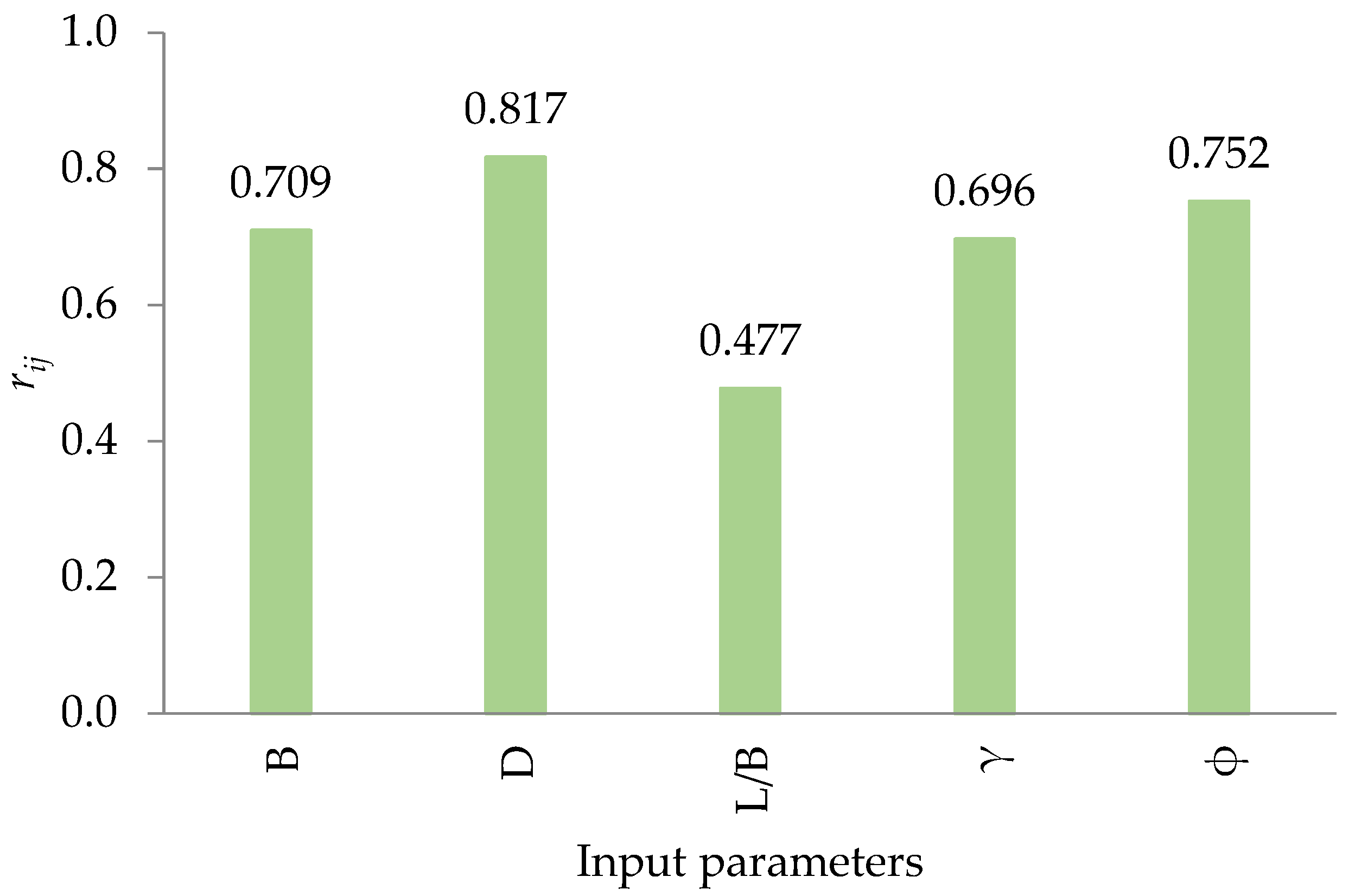
3.2. Correlation Analysis
3.3. Gaussian Processes Regression
3.4. Model Evaluation and Comparison
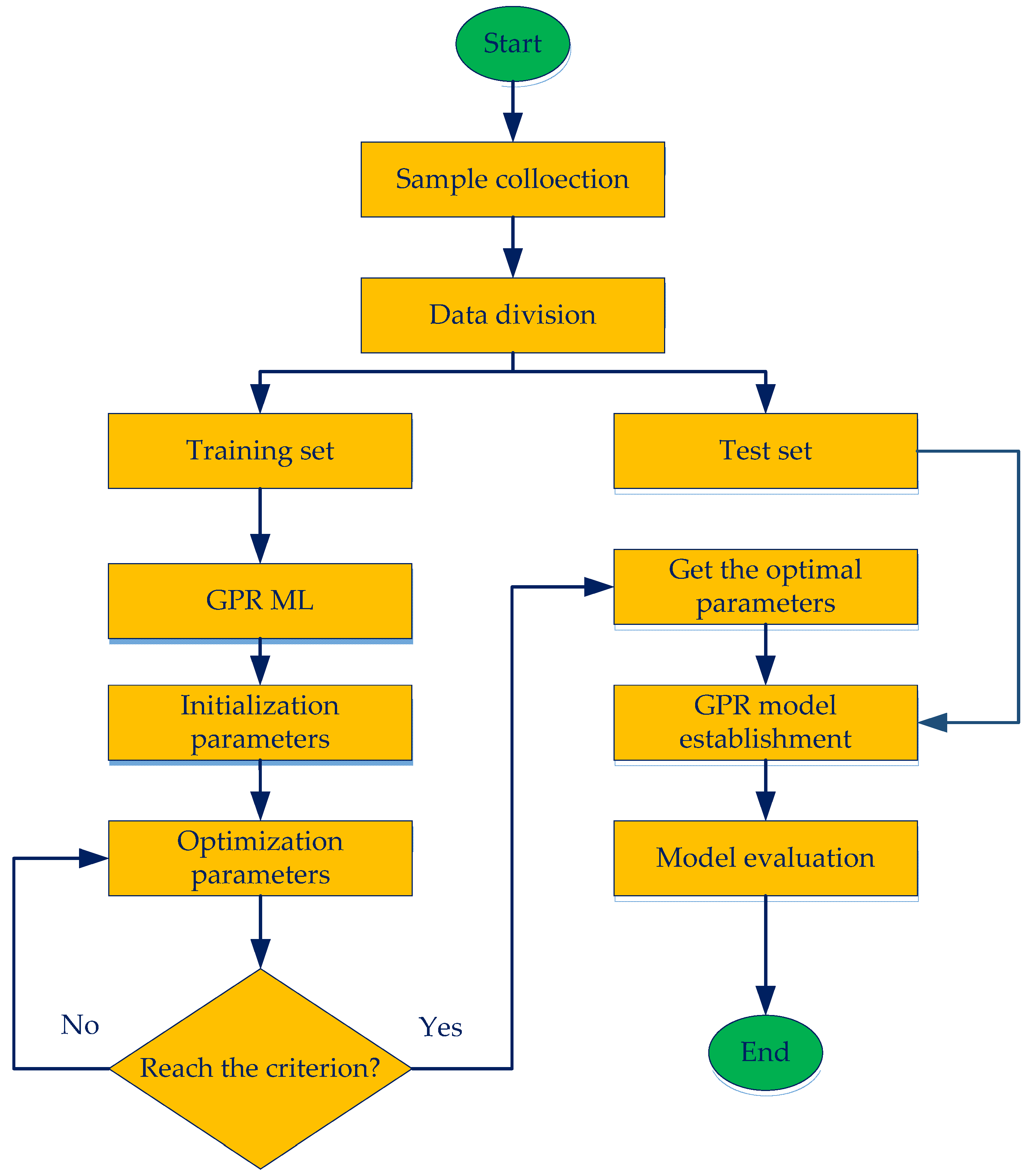
4. Construction of Prediction Model
5. Results and Discussion
6. Conclusions
Author Contributions
Funding
Institutional Review Board Statement
Informed Consent Statement
Data Availability Statement
Conflicts of Interest
Appendix A

| S. No. | B (m) | D (m) | L/B | γ (kN/m3) | ϕ (°) | qu (kPa) |
|---|---|---|---|---|---|---|
| 1 | 0.6 | 0.3 | 2 | 9.85 | 34.9 | 270 |
| 2 | 0.6 | 0 | 2 | 10.85 | 44.8 | 860 |
| 3 | 0.152 | 0.075 | 5.95 | 17.1 | 42.5 | 335.3 |
| 4 | 0.0585 | 0.058 | 5.95 | 16.8 | 41.5 | 184.9 |
| 5 | 0.5 | 0 | 1 | 11.7 | 37 | 111 |
| 6 | 0.5 | 0 | 2 | 11.7 | 37 | 143 |
| 7 * | 0.5 | 0.3 | 1 | 10.2 | 37.7 | 681 |
| 8 | 0.152 | 0.15 | 1 | 16.1 | 37 | 182.4 |
| 9 | 0.0585 | 0.058 | 5.95 | 15.7 | 34 | 70.91 |
| 10 * | 1 | 0 | 3 | 11.93 | 40 | 630 |
| 11 | 0.152 | 0.15 | 5.95 | 15.7 | 34 | 122.3 |
| 12 | 0.152 | 0.15 | 1 | 16.8 | 41.5 | 361.5 |
| 13 * | 0.5 | 0.5 | 4 | 12 | 40 | 1140 |
| 14 | 0.5 | 0.029 | 4 | 11.7 | 37 | 109 |
| 15 | 0.5 | 0 | 1 | 10.2 | 37.7 | 154 |
| 16 | 0.094 | 0.094 | 6 | 17.1 | 42.5 | 279.6 |
| 17 | 0.094 | 0.047 | 1 | 16.1 | 37 | 98.8 |
| 18 | 0.5 | 0.5 | 2 | 12.41 | 44 | 2847 |
| 19 | 0.5 | 0 | 4 | 12.41 | 44 | 797 |
| 20 | 0.0585 | 0.029 | 5.95 | 16.1 | 37 | 82.5 |
| 21 * | 0.152 | 0.075 | 1 | 16.1 | 37 | 135.2 |
| 22 | 0.5 | 0.3 | 1 | 12.41 | 44 | 1940 |
| 23 * | 0.152 | 0.15 | 1 | 16.5 | 39.5 | 264.5 |
| 24 | 0.5 | 0 | 2 | 10.2 | 37.7 | 195 |
| 25 * | 0.6 | 0.3 | 2 | 10.85 | 44.8 | 1760 |
| 26 | 0.991 | 0.711 | 1 | 15.8 | 32 | 1773.7 |
| 27 | 0.5 | 0.3 | 1 | 11.7 | 37 | 446 |
| 28 | 0.5 | 0 | 1 | 10.2 | 37.7 | 165 |
| 29 | 0.5 | 0 | 1 | 11.77 | 37 | 123 |
| 30 | 0.5 | 0.49 | 4 | 12.27 | 42 | 1492 |
| 31 | 0.152 | 0.15 | 5.95 | 16.8 | 41.5 | 342.5 |
| 32 | 0.094 | 0.094 | 6 | 16.5 | 39.5 | 185.6 |
| 33 | 0.5 | 0 | 1 | 11.7 | 37 | 132 |
| 34 | 0.5 | 0 | 2 | 10.2 | 37.7 | 203 |
| 35 * | 0.5 | 0.3 | 4 | 11.7 | 37 | 322 |
| 36 | 0.094 | 0.094 | 1 | 15.7 | 34 | 90.5 |
| 37 | 0.094 | 0.047 | 6 | 16.8 | 41.5 | 206.8 |
| 38 | 0.094 | 0.047 | 6 | 16.1 | 37 | 104.8 |
| 39 | 2.489 | 0.762 | 1 | 15.8 | 32 | 1158 |
| 40 | 0.094 | 0.094 | 1 | 16.5 | 39.5 | 191.6 |
| 41 | 0.152 | 0.075 | 5.95 | 15.7 | 34 | 98.2 |
| 42 | 0.094 | 0.047 | 1 | 16.5 | 39.5 | 147.8 |
| 43 | 0.5 | 0.127 | 4 | 11.7 | 37 | 187 |
| 44 * | 0.5 | 0.5 | 4 | 12.41 | 44 | 2033 |
| 45 * | 0.094 | 0.094 | 1 | 16.8 | 41.5 | 253.6 |
| 46 | 0.5 | 0.3 | 3 | 10.2 | 37.7 | 402 |
| 47 | 3.004 | 0.762 | 1 | 15.8 | 32 | 1019.4 |
| 48 | 0.152 | 0.075 | 1 | 16.8 | 41.5 | 276.3 |
| 49 | 0.094 | 0.047 | 6 | 17.1 | 42.5 | 235.6 |
| 50 | 0.152 | 0.15 | 5.95 | 16.1 | 37 | 176.4 |
| 51 | 0.6 | 0.3 | 2 | 10.2 | 37.7 | 570 |
| 52 | 0.5 | 0.3 | 1 | 11.77 | 37 | 370 |
| 53 | 0.5 | 0.3 | 2 | 10.2 | 37.7 | 530 |
| 54 | 0.094 | 0.047 | 1 | 16.8 | 41.5 | 196.8 |
| 55 * | 0.094 | 0.094 | 6 | 16.8 | 41.5 | 244.6 |
| 56 | 0.094 | 0.094 | 1 | 17.1 | 42.5 | 295.6 |
| 57 | 0.152 | 0.15 | 5.95 | 16.5 | 39.5 | 254.5 |
| 58 | 0.52 | 0 | 3.85 | 10.2 | 37.7 | 186 |
| 59 | 0.152 | 0.15 | 5.95 | 17.1 | 42.5 | 400.6 |
| 60 | 1 | 0.2 | 3 | 11.97 | 39 | 710 |
| 61 | 0.0585 | 0.029 | 5.95 | 15.7 | 34 | 58.5 |
| 62 * | 0.5 | 0.013 | 1 | 11.7 | 37 | 137 |
| 63 | 0.5 | 0.3 | 1 | 12.41 | 44 | 2266 |
| 64 | 0.0585 | 0.029 | 5.95 | 16.5 | 39.5 | 121.5 |
| 65 | 0.5 | 0.5 | 4 | 11.7 | 37 | 425 |
| 66 | 0.094 | 0.094 | 6 | 16.1 | 37 | 127.5 |
| 67 * | 0.0585 | 0.029 | 5.95 | 17.1 | 42.5 | 180.5 |
| 68 | 0.152 | 0.075 | 1 | 15.7 | 34 | 91.2 |
| 69 * | 0.152 | 0.075 | 5.95 | 16.1 | 37 | 143.3 |
| 70 | 0.094 | 0.047 | 1 | 15.7 | 34 | 67.7 |
| 71 | 0.152 | 0.075 | 1 | 17.1 | 42.5 | 325.3 |
| 72 | 0.094 | 0.047 | 1 | 17.1 | 42.5 | 228.8 |
| 73 | 0.5 | 0.3 | 2 | 10.2 | 37.7 | 542 |
| 74 | 0.094 | 0.047 | 6 | 15.7 | 34 | 74.7 |
| 75 | 0.094 | 0.047 | 6 | 16.5 | 39.5 | 155.8 |
| 76 * | 1.492 | 0.762 | 1 | 15.8 | 32 | 1540 |
| 77 | 0.5 | 0 | 1 | 12.41 | 44 | 782 |
| 78 | 0.6 | 0 | 2 | 10.2 | 37.7 | 200 |
| 79 | 0.152 | 0.075 | 5.95 | 16.5 | 39.5 | 211.2 |
| 80 | 0.5 | 0.5 | 2 | 11.7 | 37 | 565 |
| 81 | 0.152 | 0.15 | 1 | 17.1 | 42.5 | 423.6 |
| 82 * | 0.5 | 0.5 | 2 | 11.77 | 37 | 464 |
| 83 | 0.152 | 0.075 | 5.95 | 16.8 | 41.5 | 285.3 |
| 84 * | 0.094 | 0.094 | 1 | 16.1 | 37 | 131.5 |
| 85 | 0.0585 | 0.058 | 5.95 | 17.1 | 42.5 | 211 |
| 86 | 0.152 | 0.075 | 1 | 16.5 | 39.5 | 201.2 |
| 87 | 0.0585 | 0.058 | 5.95 | 16.5 | 39.5 | 142.9 |
| 88 | 0.0585 | 0.058 | 5.95 | 16.1 | 37 | 98.93 |
| 89 | 0.152 | 0.15 | 1 | 15.7 | 34 | 124.4 |
| 90 * | 0.5 | 0 | 3 | 10.2 | 37.7 | 214 |
| 91 | 0.0585 | 0.029 | 5.95 | 16.8 | 41.5 | 157.5 |
| 92 * | 0.094 | 0.094 | 6 | 15.7 | 34 | 91.5 |
| 93 * | 0.5 | 0 | 4 | 12 | 40 | 461 |
| 94 | 0.52 | 0.3 | 3.85 | 10.2 | 37.7 | 413 |
| 95 | 3.016 | 0.889 | 1 | 15.8 | 32 | 1161.2 |
| 96 | 0.5 | 0 | 2 | 11.77 | 37 | 134 |
| 97 | 0.5 | 0.3 | 1 | 11.7 | 37 | 406 |
References
- Terzaghi, K. Theoretical Soil Mechanics; John Wiley and Sons: New York, NY, USA, 1943. [Google Scholar]
- Meyerhof, G.G. Some recent research on the bearing capacity of foundations. Can. Geotech. J. 1963, 1, 16–26. [Google Scholar] [CrossRef]
- Hansen, J.B. A Revised and Extended Formula for Bearing Capacity; Danish Geotechnical Institute: Lyngby, Denmark, 1970. [Google Scholar]
- Vesic, A. Bearing Capacity of Shallow Foundations. In Foundation Engineering Handbook; Winterkorn, F.S., Fand, H.Y., Eds.; Van Nostrand Reinhold: New York, NY, USA, 1975. [Google Scholar]
- Das, B. Principles of Foundation Engineering; Brooks/Cole-Thomson Learning, Inc.: Boston, MA, USA, 2004; p. 489. [Google Scholar]
- Conte, E.; Pugliese, L.; Troncone, A.; Vena, M. A simple approach for evaluating the bearing capacity of piles subjected to inclined loads. Int. J. Geomech. 2021, 21, 04021224. [Google Scholar] [CrossRef]
- Achmus, M.; Thieken, K. On the behavior of piles in non-cohesive soil under combined horizontal and vertical loading. Acta Geotechnica 2010, 5, 199–210. [Google Scholar] [CrossRef]
- De Beer, E. The scale effect on the phenomenon of progressive rupture in cohesionless soils. In Proceedings of the 6th ICSMFE, Montreal, QC, Canada, 8–15 September 1965; pp. 13–17. [Google Scholar]
- Yamaguchi, H. On the scale effect of footings in dense sand. In Proceedings of the 9th ICSMFE, Tokyo, Japan, 10–15 July 1977; pp. 795–798. [Google Scholar]
- Tatsuoka, T. Progressive failure and particle size effect in bearing capacity of footing on sand. ASCE Geotech. Spec. Publ. 1991, 27, 788–802. [Google Scholar]
- Padmini, D.; Ilamparuthi, K.; Sudheer, K. Ultimate bearing capacity prediction of shallow foundations on cohesionless soils using neurofuzzy models. Comput. Geotech. 2008, 35, 33–46. [Google Scholar] [CrossRef]
- Ahmad, M.; Tang, X.-W.; Qiu, J.-N.; Ahmad, F. Evaluation of liquefaction-induced lateral displacement using Bayesian belief networks. Front. Struct. Civ. Eng. 2021, 15, 80–98. [Google Scholar] [CrossRef]
- Ali Khan, M.; Zafar, A.; Akbar, A.; Javed, M.F.; Mosavi, A. Application of Gene Expression Programming (GEP) for the Prediction of Compressive Strength of Geopolymer Concrete. Materials 2021, 14, 1106. [Google Scholar] [CrossRef] [PubMed]
- Ahmad, M.; Hu, J.-L.; Ahmad, F.; Tang, X.-W.; Amjad, M.; Iqbal, M.J.; Asim, M.; Farooq, A. Supervised Learning Methods for Modeling Concrete Compressive Strength Prediction at High Temperature. Materials 2021, 14, 1983. [Google Scholar] [CrossRef] [PubMed]
- Ahmad, M.; Tang, X.-W.; Qiu, J.-N.; Gu, W.-J.; Ahmad, F. A hybrid approach for evaluating CPT-based seismic soil liquefaction potential using Bayesian belief networks. J. Cent. South Univ. 2020, 27, 500–516. [Google Scholar]
- Pirhadi, N.; Tang, X.; Yang, Q.; Kang, F. A new equation to evaluate liquefaction triggering using the response surface method and parametric sensitivity analysis. Sustainability 2019, 11, 112. [Google Scholar] [CrossRef] [Green Version]
- Ahmad, M.; Tang, X.; Ahmad, F. Evaluation of Liquefaction-Induced Settlement Using Random Forest and REP Tree Models: Taking Pohang Earthquake as a Case of Illustration. In Natural Hazards-Impacts, Adjustments & Resilience; IntechOpen: London, UK, 2020. [Google Scholar]
- Ahmad, M.; Al-Shayea, N.A.; Tang, X.-W.; Jamal, A.; Al-Ahmadi, H.M.; Ahmad, F. Predicting the Pillar Stability of Underground Mines with Random Trees and C4. 5 Decision Trees. Appl. Sci. 2020, 10, 6486. [Google Scholar] [CrossRef]
- Ahmad, M.; Tang, X.-W.; Qiu, J.-N.; Ahmad, F.; Gu, W.-J. A step forward towards a comprehensive framework for assessing liquefaction land damage vulnerability: Exploration from historical data. Front. Struct. Civ. Eng. 2020, 14, 1476–1491. [Google Scholar] [CrossRef]
- Zhou, J.; Li, E.; Wang, M.; Chen, X.; Shi, X.; Jiang, L. Feasibility of stochastic gradient boosting approach for evaluating seismic liquefaction potential based on SPT and CPT case histories. J. Perform. Constr. Facil. 2019, 33, 04019024. [Google Scholar] [CrossRef]
- Hamdia, K.M.; Arafa, M.; Alqedra, M. Structural damage assessment criteria for reinforced concrete buildings by using a Fuzzy Analytic Hierarchy process. Undergr. Space 2018, 3, 243–249. [Google Scholar] [CrossRef]
- Kalinli, A.; Acar, M.C.; Gündüz, Z. New approaches to determine the ultimate bearing capacity of shallow foundations based on artificial neural networks and ant colony optimization. Eng. Geol. 2011, 117, 29–38. [Google Scholar] [CrossRef]
- Samui, P. Application of statistical learning algorithms to ultimate bearing capacity of shallow foundation on cohesionless soil. Int. J. Numer. Anal. Methods Geomech. 2012, 36, 100–110. [Google Scholar] [CrossRef]
- Shahnazari, H.; Tutunchian, M.A. Prediction of ultimate bearing capacity of shallow foundations on cohesionless soils: An evolutionary approach. KSCE J. Civ. Eng. 2012, 16, 950–957. [Google Scholar] [CrossRef]
- Tsai, H.-C.; Tyan, Y.-Y.; Wu, Y.-W.; Lin, Y.-H. Determining ultimate bearing capacity of shallow foundations using a genetic programming system. Neural Comput. Appl. 2013, 23, 2073–2084. [Google Scholar] [CrossRef]
- Kohestani, V.R.; Vosoghi, M.; Hassanlourad, M.; Fallahnia, M. Bearing capacity of shallow foundations on cohesionless soils: A random forest based approach. Civ. Eng. Infrastruct. J. 2017, 50, 35–49. [Google Scholar]
- Hewing, L.; Kabzan, J.; Zeilinger, M.N. Cautious model predictive control using gaussian process regression. IEEE Trans. Control. Syst. Technol. 2019, 28, 2736–2743. [Google Scholar] [CrossRef] [Green Version]
- Sun, A.Y.; Wang, D.; Xu, X. Monthly streamflow forecasting using Gaussian process regression. J. Hydrol. 2014, 511, 72–81. [Google Scholar] [CrossRef]
- Roushangar, K.; Shahnazi, S. Prediction of sediment transport rates in gravel-bed rivers using Gaussian process regression. J. Hydroinform. 2020, 22, 249–262. [Google Scholar] [CrossRef]
- Prandtl, L. On the penetrating strengths (hardness) of plastic construction materials and the strength of cutting edges. ZAMM J. Appl. Math. Mech. 1921, 1, 15–20. [Google Scholar] [CrossRef]
- Reissner, H. Zum erddruckproblem. In Proceedings of the 1st International Congress for Applied Mechanics, Delft, The Netherlands, 22–26 April 1924; pp. 295–311. [Google Scholar]
- Taylor, D. Fundamentals of Soil Mechanics; John Wiley & Sons: New York, NY, USA; Chapman & Hall: London, UK, 1948. [Google Scholar]
- Vesić, A.S. Analysis of ultimate loads of shallow foundations. J. Soil Mech. Found. Div. 1973, 99, 45–73. [Google Scholar] [CrossRef]
- Cerato, A. Scale Effects of Foundation Bearing Capacity on Granular Material. Ph.D. Dissertation, Lafayette College, University of Massachusetts Amherst, Amherst, MA, USA, 2005. [Google Scholar]
- Ahmad, M.; Tang, X.-W.; Qiu, J.-N.; Ahmad, F. Evaluating Seismic Soil Liquefaction Potential Using Bayesian Belief Network and C4. 5 Decision Tree Approaches. Appl. Sci. 2019, 9, 4226. [Google Scholar] [CrossRef] [Green Version]
- Javadi, A.A.; Rezania, M.; Nezhad, M.M. Evaluation of liquefaction induced lateral displacements using genetic programming. Comput. Geotech. 2006, 33, 222–233. [Google Scholar] [CrossRef]
- Van Vuren, T. Modeling of Transport Demand–Analyzing, Calculating, and Forecasting Transport Demand; Elsevier: Amsterdam, The Netherlands, 2018; p. 472. [Google Scholar]
- Song, Y.; Gong, J.; Gao, S.; Wang, D.; Cui, T.; Li, Y.; Wei, B. Susceptibility assessment of earthquake-induced landslides using Bayesian network: A case study in Beichuan, China. Comput. Geosci. 2012, 42, 189–199. [Google Scholar] [CrossRef]
- Zhao, K.; Popescu, S.; Meng, X.; Pang, Y.; Agca, M. Characterizing forest canopy structure with lidar composite metrics and machine learning. Remote Sens. Environ. 2011, 115, 1978–1996. [Google Scholar] [CrossRef]
- Pasolli, L.; Melgani, F.; Blanzieri, E. Gaussian process regression for estimating chlorophyll concentration in subsurface waters from remote sensing data. IEEE Geosci. Remote Sens. Lett. 2010, 7, 464–468. [Google Scholar] [CrossRef]
- Rasmussen, C.; Williams, C. Gaussian Processes for Machine Learning; The MIT Press: Cambridge, MA, USA, 2006; Volume 35, pp. 715–719. [Google Scholar]
- Bazi, Y.; Alajlan, N.; Melgani, F.; AlHichri, H.; Yager, R.R. Robust estimation of water chlorophyll concentrations with gaussian process regression and IOWA aggregation operators. IEEE J. Sel. Top. Appl. Earth Obs. Remote Sens. 2014, 7, 3019–3028. [Google Scholar] [CrossRef]
- Kumar, M.; Elbeltagi, A.; Srivastava, A.; Kumari, A.; Ali, R.; Pande, C.; Bajirao, T.S.; Islam, A.R.M.T.; Kushwaha, D.P. Prediction of Daily Streamflow Using Various Kernel Function Based Regression: A Case Study in India. Preprint. 2021. Available online: https://assets.researchsquare.com/files/rs-784271/v1_covered.pdf?c=1631876022 (accessed on 24 September 2021).
- Gandomi, A.H.; Babanajad, S.K.; Alavi, A.H.; Farnam, Y. Novel approach to strength modeling of concrete under triaxial compression. J. Mater. Civ. Eng. 2012, 24, 1132–1143. [Google Scholar] [CrossRef]
- Nush, J.; Sutcliffe, J.V. River flow forecasting through conceptual models part I—A discussion of principles. J. Hydrol. 1970, 10, 282–290. [Google Scholar] [CrossRef]
- Moriasi, D.N.; Arnold, J.G.; van Liew, M.W.; Bingner, R.L.; Harmel, R.D.; Veith, T.L. Model evaluation guidelines for systematic quantification of accuracy in watershed simulations. Trans. ASABE 2007, 50, 885–900. [Google Scholar] [CrossRef]
- Khosravi, K.; Mao, L.; Kisi, O.; Yaseen, Z.M.; Shahid, S. Quantifying hourly suspended sediment load using data mining models: Case study of a glacierized Andean catchment in Chile. J. Hydrol. 2018, 567, 165–179. [Google Scholar] [CrossRef]
- Witten, I.H.; Frank, E.; Hall, M. Data Mining: Practical Machine Learning Tools and Techniques; Morgen Kaufmann: San Francisco, CA, USA, 2005. [Google Scholar]
- Üstün, B.; Melssen, W.J.; Buydens, L.M. Facilitating the application of support vector regression by using a universal Pearson VII function based kernel. Chemom. Intellig. Lab. Syst. 2006, 81, 29–40. [Google Scholar] [CrossRef]
- Vesić, A.S. Closure to “Analysis of Ultimate Loads of Shallow Foundations”. J. Geotech. Eng. Div. 1974, 100, 949–952. [Google Scholar] [CrossRef]
- Yang, Y.; Zhang, Q. A hierarchical analysis for rock engineering using artificial neural networks. Rock Mech. Rock Eng. 1997, 30, 207–222. [Google Scholar] [CrossRef]
- Faradonbeh, R.S.; Armaghani, D.J.; Abd Majid, M.; Tahir, M.M.; Murlidhar, B.R.; Monjezi, M.; Wong, H. Prediction of ground vibration due to quarry blasting based on gene expression programming: A new model for peak particle velocity prediction. Int. J. Environ. Sci. Technol. 2016, 13, 1453–1464. [Google Scholar] [CrossRef] [Green Version]
- Chen, W.; Hasanipanah, M.; Rad, H.N.; Armaghani, D.J.; Tahir, M. A new design of evolutionary hybrid optimization of SVR model in predicting the blast-induced ground vibration. Eng. Comput. 2021, 37, 1455–1471. [Google Scholar] [CrossRef]
- Rad, H.N.; Bakhshayeshi, I.; Jusoh, W.A.W.; Tahir, M.; Foong, L.K. Prediction of flyrock in mine blasting: A new computational intelligence approach. Nat. Resour. Res. 2020, 29, 609–623. [Google Scholar]


| Reference | Equation |
|---|---|
| Terzaghi [1] | |
| Meyerhof [2] | |
| Hansen [3] | = same as Meyerhof above = same as Meyerhof above |
| Vesic [4] | Same as Hansen’s equation = same as Meyerhof above = same as Meyerhof above |
| Dataset | Statistical Parameter | B (m) | D (m) | L/B | γ (kN/m3) | ϕ (°) | qu (kPa) |
|---|---|---|---|---|---|---|---|
| Training | Minimum | 0.0585 | 0 | 1 | 9.85 | 32 | 58.5 |
| Maximum | 3.016 | 0.889 | 6 | 17.1 | 44.8 | 2847 | |
| Mean | 0.398 | 0.156 | 3.126 | 14.279 | 38.492 | 407.899 | |
| Standard deviation | 0.543 | 0.195 | 2.192 | 2.642 | 3.308 | 511.870 | |
| Testing | Minimum | 0.0585 | 0 | 1 | 10.2 | 32 | 91.5 |
| Maximum | 1.492 | 0.762 | 6 | 17.1 | 44.8 | 2033 | |
| Mean | 0.420 | 0.204 | 2.995 | 13.777 | 38.800 | 569.826 | |
| Standard deviation | 0.361 | 0.221 | 1.964 | 2.573 | 3.225 | 600.020 |
| Parameter | B | D | L/B | γ | ϕ | qu |
|---|---|---|---|---|---|---|
| B | 1.000 | |||||
| D | 0.710 | 1.000 | ||||
| L/B | −0.351 | −0.249 | 1.000 | |||
| γ | −0.269 | −0.125 | 0.340 | 1.000 | ||
| ϕ | −0.378 | −0.286 | 0.124 | 0.076 | 1.000 | |
| qu | 0.452 | 0.671 | −0.248 | −0.238 | 0.258 | 1.000 |
| Performance Index | Training | Testing |
|---|---|---|
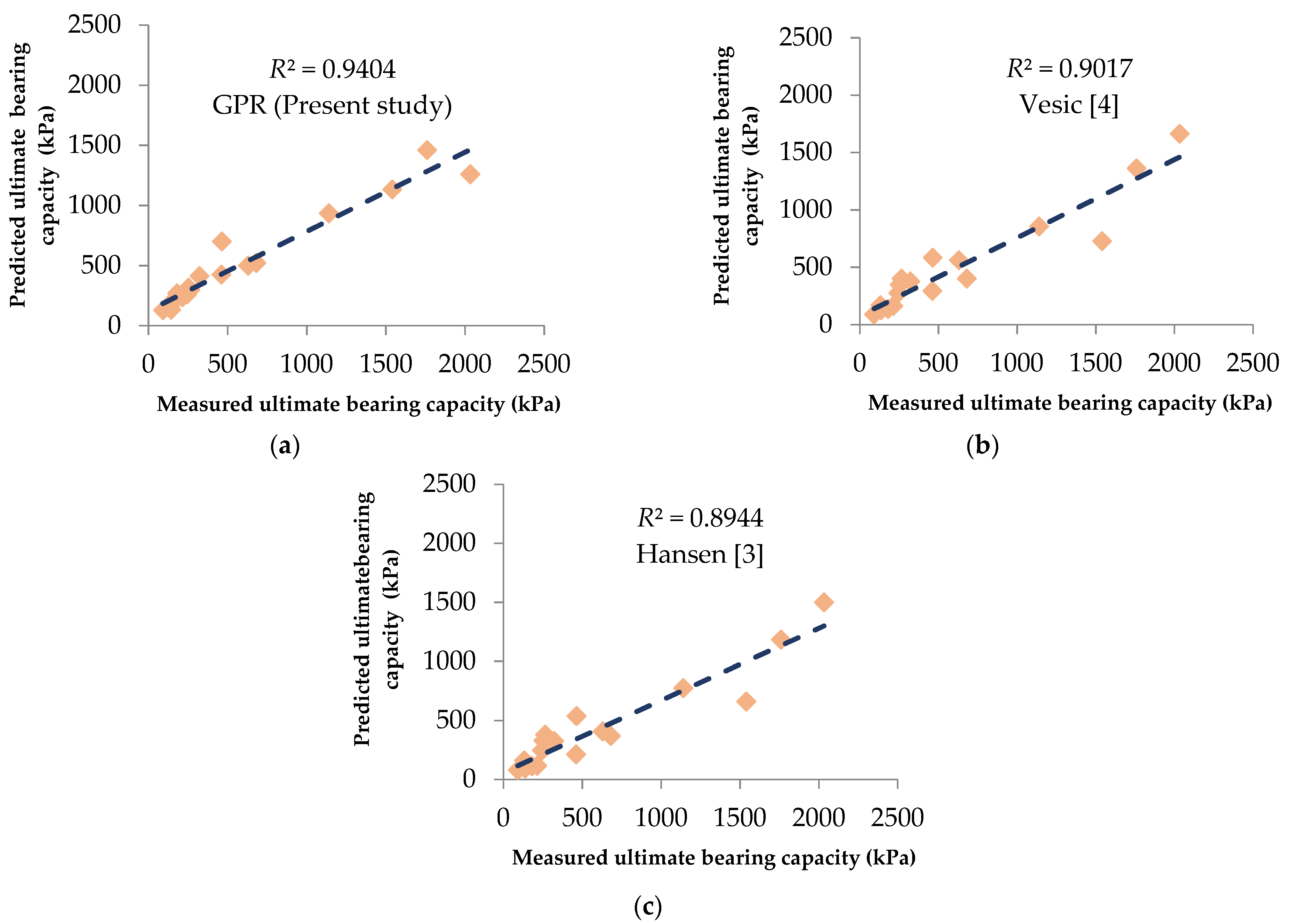
| R2 | 0.9552 | 0.9404 |
| RSR | 0.3428 | 0.3975 |
| NSE | 0.8825 | 0.8420 |
| MBE (kPa) | −10.9661 | −69.3268 |
Publisher’s Note: MDPI stays neutral with regard to jurisdictional claims in published maps and institutional affiliations. |
© 2021 by the authors. Licensee MDPI, Basel, Switzerland. This article is an open access article distributed under the terms and conditions of the Creative Commons Attribution (CC BY) license (https://creativecommons.org/licenses/by/4.0/).
Share and Cite
Ahmad, M.; Ahmad, F.; Wróblewski, P.; Al-Mansob, R.A.; Olczak, P.; Kamiński, P.; Safdar, M.; Rai, P. Prediction of Ultimate Bearing Capacity of Shallow Foundations on Cohesionless Soils: A Gaussian Process Regression Approach. Appl. Sci. 2021, 11, 10317. https://0-doi-org.brum.beds.ac.uk/10.3390/app112110317
Ahmad M, Ahmad F, Wróblewski P, Al-Mansob RA, Olczak P, Kamiński P, Safdar M, Rai P. Prediction of Ultimate Bearing Capacity of Shallow Foundations on Cohesionless Soils: A Gaussian Process Regression Approach. Applied Sciences. 2021; 11(21):10317. https://0-doi-org.brum.beds.ac.uk/10.3390/app112110317
Chicago/Turabian StyleAhmad, Mahmood, Feezan Ahmad, Piotr Wróblewski, Ramez A. Al-Mansob, Piotr Olczak, Paweł Kamiński, Muhammad Safdar, and Partab Rai. 2021. "Prediction of Ultimate Bearing Capacity of Shallow Foundations on Cohesionless Soils: A Gaussian Process Regression Approach" Applied Sciences 11, no. 21: 10317. https://0-doi-org.brum.beds.ac.uk/10.3390/app112110317