
Evaluation of a Novel Condition Indicator with Comparative Application to Hypoid Gear Failures


1
Direct Line Kft., 2330 Dunaharaszti, Hungary
2
AVL List GmbH, 8020 Graz, Austria
3
iba AG, 90762 Fürth, Germany
4
IME (Institute of Machine Components), TU Graz (Graz University of Technology), 8010 Graz, Austria
*
Author to whom correspondence should be addressed.
Appl. Sci. 2021, 11(23), 11499; https://0-doi-org.brum.beds.ac.uk/10.3390/app112311499
Submission received: 24 October 2021
/
Revised: 21 November 2021
/
Accepted: 23 November 2021
/
Published: 4 December 2021
(This article belongs to the Special Issue Alternative Techniques in Vibration Measurement and Analysis)
Abstract
:This paper presents a condition monitoring methodology that uses a novel condition indicator (CI) algorithm, allowing for a confident assessment of system health and an advanced warning of failures. The CI is evaluated in the application of a specialized gear rig utilized for the high-cycle fatigue testing of hypoid gears. The CI is shown in this case study to ensure higher confidence in the prediction of failures than other algorithms, with variations in the results. In the comparison, consideration is given to the signal-to-noise ratio, the ability to differentiate between damages and/or damaged components and the sensitivity of the CI to the failure.
1. Introduction
Condition monitoring (CM), when correctly applied, offers high potential savings on the costs of equipment downtime and repair. By identifying system damages before failures occur, maintenance can be changed from “responsive” to “planned” and the secondary damages that so often accompany failures can be avoided completely. It is estimated that the total cost of downtime in the UK manufacturing industry could be as high as GBP 180bn annually [1,2], where the total estimated costs of repairs and downtime are estimated to be between 15% and 60% [3,4,5,6]. Moving from responsive to planned maintenance has been shown to reduce costs significantly [7,8].
The condition monitoring of the hypoid gear during testing, as described in the current study, is an example of a CM approach in the automotive testing industry, which can be applied to other fields as well.
Naturally, the cost of sensor equipment and monitoring should be considered and offset against the potential savings and, therefore, condition monitoring has conventionally been limited to high-value equipment. This convention is due to change as sensor networks, data transfer and processing are all decreasing in cost and improving in quality. Indeed, many high-value manufacturing industries already have the necessary equipment incorporated into their systems for control, protection and other features. These systems only lack the application of CM as the key components of a CM system already exist within the assembly.
One such application area is electrified automotive drivelines, especially in the design validation phases of testing, which include many thermal sensors as well as e-motor rotor angular resolvers as standard and already have the on-board monitoring capabilities within the control units. For such industries, the missing link in achieving the potential savings is largely down to the identification of condition indicators (CI) capable of accurately and consistently identifying failures. Several CI have been shown in publications for a range of applications [9]; however, a comparison is lacking to assist in selecting a suitable CI for a given application.
This paper will introduce a new CI that is applicable to a wide range of gear monitoring applications but developed with isolated automotive component-level testing. Using recorded test data from several lifetime fatigue tests, the new CI can be compared to many other available CI options to evaluate the key performance attributes needed from CM. Consideration is given to the signal-to-noise ratio, the ability to differentiate between damages and/or damaged components and the sensitivity of the CI to the failure. Through this comparison, it can be shown that some CI algorithms are not suitable for application without a detailed calibration and filtering of the signals, whereas others can produce clear and repeatable trends that reduce the risk of false flags and support the diagnosis and prognosis of the system’s health.
The goal of this paper, based on [10], is not to assess precisely how the crack propagation and breakage in this specific application of CM is influenced by the CI applied. As an in-depth assessment, which would constitute frequent stops, crack detection and examinations, was not possible during the testing, the results from using the CI and the documentation of the damage are summarized to allow for the evaluation of the capabilities and weaknesses of the CI options evaluated. This paper presents an in situ test of the algorithm in an industrial application, where the damage of the components cannot be foreseen and the method is assessed to determine if it can be used to effectively and reliably stop testing.
Gear crack detection is commonly described in the literature based on two approaches. One is the detection of acoustic emissions (AE) in the high-frequency domain, caused by deformation or cracking [11], which is described in [12,13]. The second and more common approach is the evaluation of vibrations, usually caused by transmission error (TE). TE is the difference between the actual instantaneous angular position of the output shaft and the position it would take if the gear were to have the perfect geometrical shape and it were a rigid bogy. A definition of TE can be found in [14], together with an explanation of the resulting system vibrations. A well known approach is to use the structure-borne noise caused by the TE for condition monitoring purposes, which is presented in [15,16,17,18,19], amongst others.
The proposed method and CI is considered to be novel as it combines the evaluation of the complete spectrum. Not only vibration signals but any arbitrary signal (in this study, torque and rotation), by comparing it to a former, undamaged state, thus eliminating the effects of the transmission path. The information of the undamaged state is retrieved—after a running in of the test specimens— in the so-called learning phase, during which the results are time-synchronously averaged to increase the signal-to-noise ratio and statistical confidence. As the calculation of the CI is not very resource intensive, it can be implemented in industrial systems.
2. Test Methodology
2.1. Application
The testing applied here was intended to investigate the fatigue lifetime of an automotive differential hypoid gearset. The conditions were selected to accelerate the test while promoting gear tooth root bending fatigue failure modes.
Differential gears play a universal and important role for automotive powertrains, almost independent of the vehicle type and drivetrain system. Hypoid gears are widely used in this context, to drive the differential gear and hence are an integral element of the drivetrain. Hypoid gears are a special group of bevel gears, with a hypoid offset, which means that the axes of the gears are crossed but not intersected. The offset of the gears can be used to optimize the packaging of the drivetrain of the vehicle while also affecting the gear face width and sliding within the contact. The definition of this offset, depending on the helix direction, and the representation of hypoid gears is depicted in Figure 1.
One main advantage of hypoid gears is the high load-carrying capacity, as in the case of pinion gears, allowing a small number of teeth and a high ratio. With the high transferred loads and good NVH behavior, this gear type provides a compromise between bevel gear and worm gear designs. However, because of the special form of the geometry, rolling and sliding occur as a relative motion while meshing, which leads to losses, reducing the efficiency and increasing the risk of flank wear, pitting, scuffing and spalling [20].
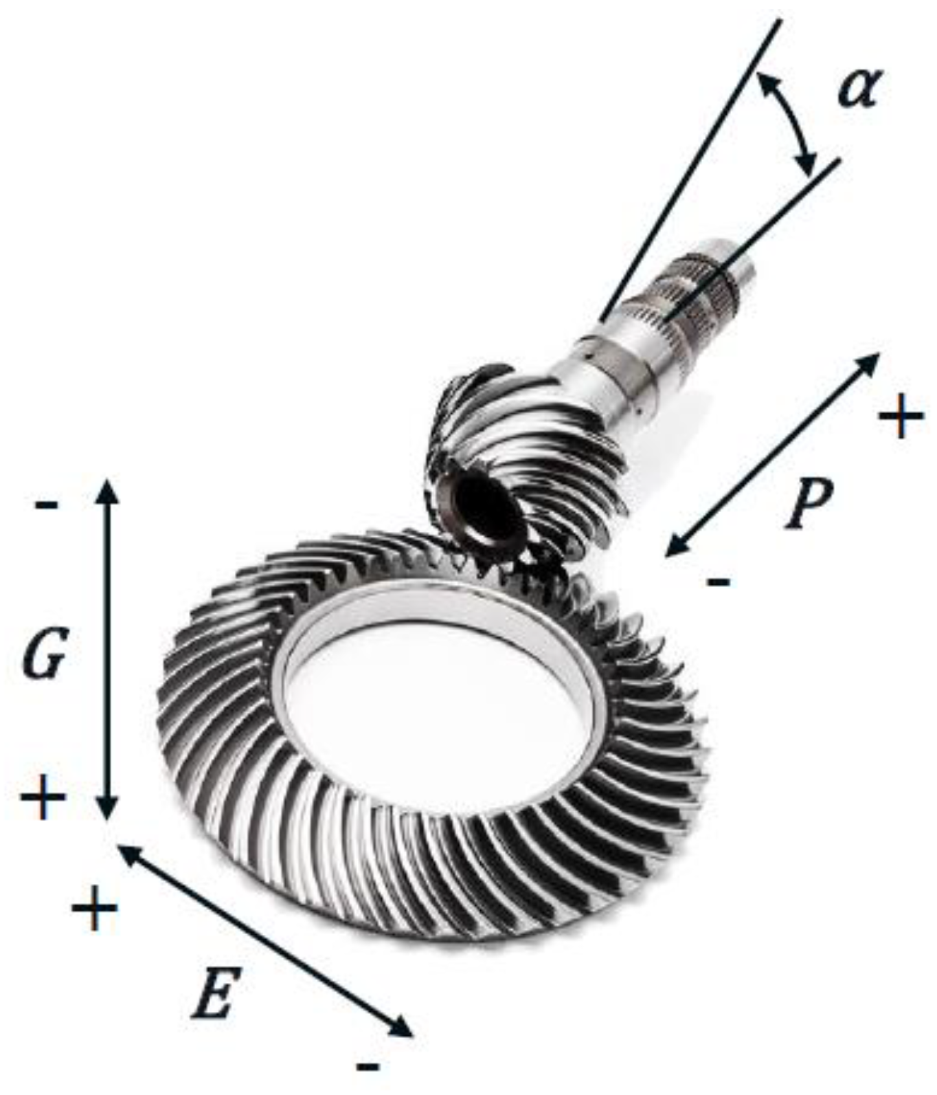
To fully utilize the advantages of hypoid gears without introducing significant losses, a very precise design and macro geometry correction is needed, which is still commonly based on “experience” with a manual variation of parameters [21]. Moreover, the contact pattern, important for the NVH behavior and for the fatigue life, varies with an increasing load because the relative positions of the pinion gear and the ring gear change, due to the stiffness of the bearings and housings in the assembly. This relative position can be defined by 4 variables, depicted in Figure 2 and represented by the letters E, P, G, . P is defined as the axis of the pinion, G as the axis of the gear, E is the shortest distance between the the P and G axes and is the angle between P and G about the E axis. Prefixing any of these terms with indicates the difference in the relative ring gear and pinion positions compared to the unloaded state.
These parameters (EPG) are not fixed but variable with torque, speed and temperature. Additionally, wear during operation leads to an evolution of the contact pattern, micro-geometry and reaction forces over time, further complicating the system response.
2.2. Test Facility
For effective and responsive testing of hypoid gears, a test bed capable of adjusting and maintaining the system variables while also supporting collection of crucial data is essential. The unique test bed utilized for this is the so-called “Specialized Gear Rig” (Figure 3), which is located at the AVL-TU Graz Transmission Center [21]. This rig is capable of applying a wide range of speeds and torques for isolated component/failure mode testing, as well as conditioning of the sample environment and responsive adjustment of EPG during operation.
This rig provides a valuable platform for development of a condition monitoring system as it allows the effective isolation of failure modes by providing a highly controlled and responsive test condition and flexibility in the test set-up. Tooth root bending fatigue is one failure mode that can be isolated easily at the test bed, where condition monitoring and crack detection play an important role.
In addition to failure mode isolation, the rig also allows the measurement of the unloaded (kinematic) TE or loaded (dynamic) TE through high-resolution angular position instrumentation. The measurement of TE provides an additional variable that can be utilized by a condition monitoring system for the evaluation of system health. The task of dynamic TE measurement was handled by the CM System (CMS); however, the TE results with respect to the NVH behavior and vibration spectra will not be presented in this work. TE will be presented in the context of a variable, which can be used for CM.
The layout of the test bed is presented in Figure 4. The gears are driven by two dynos, coupled to two different gearboxes with belt drives. The pinion gear was driven by a 132 kW motor, with a rated rotational speed of 1484 RPM, connected to a gearbox with a ratio of 3.52. The crown gear was connected to a gearbox with a ratio of 7.12, coupled to a motor with a power of 200 kW and a rated speed of 1489 RPM. During testing, the gears were covered in a housing (shown in the pictures), which is connected to an oil conditioning unit. Inside the housing, an oil jet is directed into the gear mesh, which delivers conditioned lubricant.
As depicted in Figure 4, the testing is controlled by the test bed control system, which is connected to the dynos, control system of E, P, G, , oil conditioning and CMS.
2.3. Instrumentation
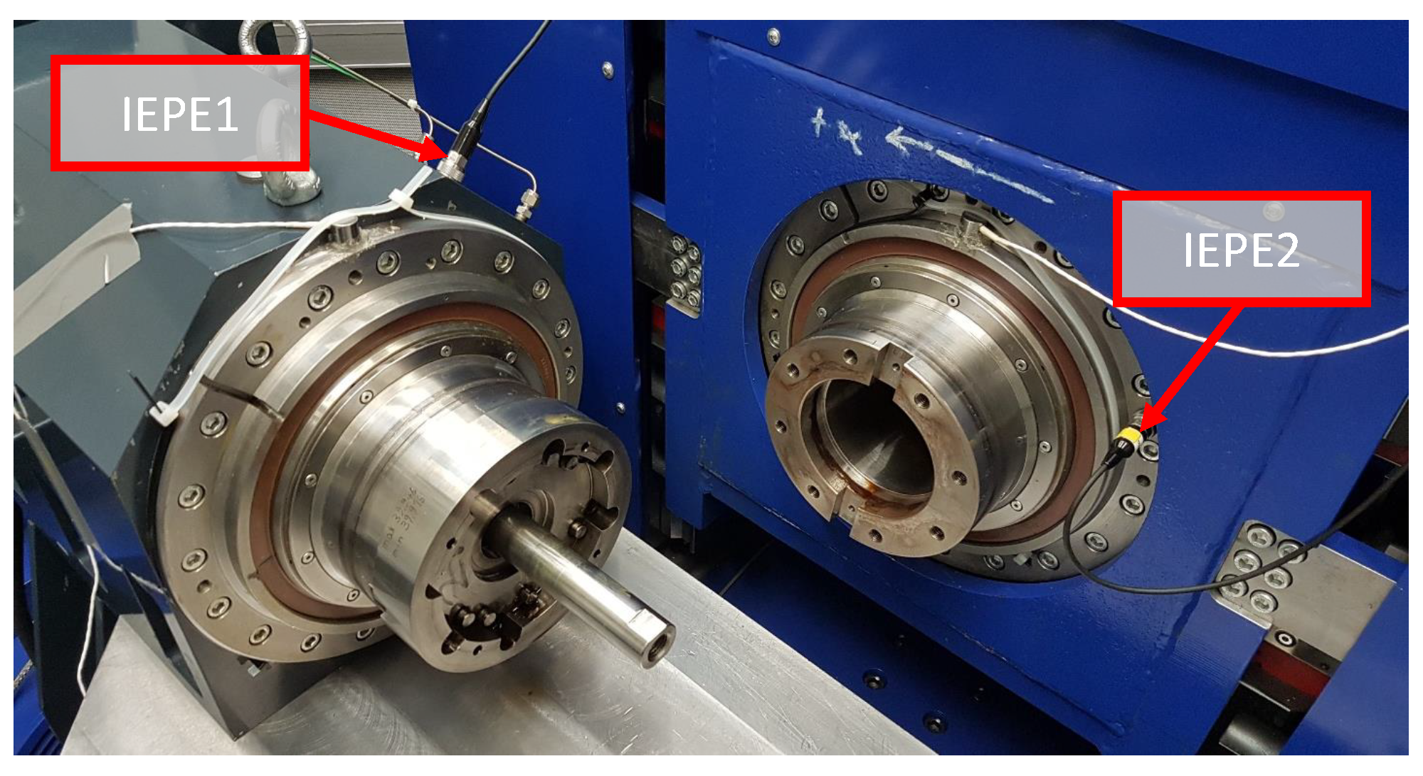
On both sides (ring and pinion gears), the torques and rotation angles are measured with the same sensor types and frequencies. Furthermore, for condition monitoring accelerometers are placed on both sides of the transmission. The sensors are shown in Figure 5. One accelerometer (IEPE1) is on the ring gear side, radially oriented to the shaft of the gear. On the pinion gear side, the accelerometer (IEPE2) is positioned axially to the drive shaft. These orientations were selected to evaluate the acceleration in the direction of the main reaction forces from the gear contact. Both sensors are fixed by magnets. A summary of the used sensors and references can be found in the Table 1.
Additionally, as shown in Figure 4, the CMS receives the torques, temperatures, and speeds at the gears via CAN-bus from the test bed control, while the rotational angle, measured at the gears, is connected directly to the CMS , . The accelerometers , are also connected directly to the CMS. Furthermore, to stop testing in case of damage, the CMS sends an analogue signal to the test bed control . Load cells are also used in determining the gear contact forces and allow a feedback loop with the tower movement to account for assembly stiffness. These load cells, which measure loads in the E, P, G and directions, are not used for condition monitoring but are crucial to correct the positioning of the samples.
The CMS consists of the ibaBM-CAN Bus monitor and the iba Modular System for the directly connected sensors. As a head-station for the iba Modular system, the ibaPADU-S-CM is used with an ibaMS8xIEPE for the IEPE sensors, an ibaMS4xADIO for analog and digital in- and outputs and an ibaMS4xUCO for incremental encoders connected via backplane bus. The hardware modules are connected via fiber optics with an industrial PC, where the signals are processed and recorded with the data-aquisition software ibaPDA. All calculations of indicators described in the following sections were carried out with the software tools ibaPDA and ibaAnalyzer, including the add-on ibaInSpectra.
2.4. Samples
The tested gear sets were produced following the current mass production method using forged alloy steel: cutting the teeth, case-hardening and lapping, optimized for bevel gears, i.e., low warping at hardening and high fatigue strength. The gear pair was applied in the rear axle of a high-power passenger car. The production process and clamping of the gears create geometrical errors when the different teeth mesh, but also every revolution of the pinion and crown wheel. This phenomenon is systematic and less visible with the latest manufacturing process, grinding or hard skiving the teeth after hardening. In the testing reported here, the ring gears had 42 teeth and the pinion gears had 13 teeth. Using a prime number creates a high variance of different tooth contacts or, a high hunting the tooth combination. This means that a high number of revolutions must be completed before a specific pair of teeth mesh again (13 revolutions of the ring gear in this case).
2.5. Testing Procedure
The testing procedure of a ring and pinion gear pair consists of several stages, starting with the assessment of the contact pattern at given loads and EPG positions, with the simultaneous measurement of the TE and contact pattern. This process essentially “tunes” the contact conditions to find the best mesh for load sharing.
After the first assessments, the relevant testing for crack and damage detection starts and the samples are loaded with a defined load and speed. The initial (unloaded) EPG values are set and the rig monitors reaction forces in order to recreate system dynamics by adjusting and maintaining EPG. After running-in for 1 h, the test specimen contact pattern is re-evaluated. If it is necessary, minor adjustments of EPG positions are made to reset the desired contact pattern. After this point, all boundary conditions (oil temperature, torque, speed, position of the gears) are constant during testing until the sample fails.
To stop testing shortly after the first fracture occurs, a preliminary version of the detailed algorithms was used together with torque monitoring. However, it was not intended to stop testing as the first crack was initiated. The goal of stopping the test was only to prohibit secondary damages because of the failure of the samples.
The same failure did not always occur, because of the variation of the loads, EPG positions and aleatoric uncertainties in the gear production (e.g., non-metalic inclusions in the material at random locations). As the test was not stopped during the run, the investigation of the failure modes and crack propagation was not possible. Furthermore, the results of metallurgical investigations are not available for all samples. However, the test data recorded allow off-line evaluation of the CM process to evaluate the effectiveness of the CI.
3. Condition Monitoring
As is described in [22], for the detection of gear cracks, the whole frequency spectrum should be monitored for changes, including increases and decreases in all amplitudes [22]. One possible algorithm is presented in [22] as the the Average-Log-Ratio (ALR) indicator, which indicates changes in the rotational harmonics. For more complex applications, not only should the harmonics of the rotational speed be monitored but also the areas in between, containing the rotational harmonics of the other components and sidebands.
To monitor these frequencies, a family of CIs has been developed and presented for ultra-low-speed applications in [23]. To prove the assumption that these CIs can be used for higher speeds, they are applied amongst other indicators in the current study for the monitoring of hypoid gears. As described in [23], the CI called the relative spectral difference () is defined, whose calculation consists of a learning phase and an evaluation phase, described below.
To determinate the RSD, the Fast-Fourier Transformation (FFT) with of an arbitrary vibration signal of interest has to be calculated, where is a vector with the FFT results for all frequencies f.
3.1. RSD Indicator
The frequency spectrum of the signal is divided into n equidistantly spread bands, up to the highest frequency monitored, , resulting in
where i is the number of the band. The frequency range for each band has to be smaller than the smallest difference between any frequencies of interest. The resulting vector contains the maximum value of for each of the bands, i. The very same FFT settings are used in the learning phase and the evaluation phase. In the learning phase, the sample is considered to be intact. The learning phase has the duration of m frequency spectra where . During the learning phase, the average and the standard deviation of the spectrum are calculated for each band in the frequency domain; , . is the vector displaying the average reference spectrum, while is a vector displaying the standard deviation for each value of for the learning phase.
With these spectra, the so-called upper and lower reference spectra are calculated, , ,
where k is the factor, which defines the distance between the upper and lower references from the . As a first approximation, it was supposed that the frequency bands have a Gaussian distribution in time and that . It must be noted that the standard deviation, more specifically the sample standard deviation, varies with the sampling time. The sample standard deviation should approximate the population standard deviation more precisely with increasing learning time. In this respect, it is important to define the learning phase correctly and, thus, determine the sample standard deviation estimating the population standard deviation well. Similar considerations are also valid for the calculation of the average.
After the learning phase, the evaluation phase begins and the relative difference between the actual spectrum and the upper and lower reference spectra , for each band can be calculated continuously, where i denotes the band.
Additionally, the maximum and minimum values over all m spectra can be learned. These references can be used to set thresholds for the automated shutdown of the test bed, but have not been used for the validation of the indicator.
Based on the relative difference for each band , the can be calculated.
Alternatively, the indicator can be calculated relative to the number of bands used:
3.2. ASD Indicator
Another approach (also described in [23]) is to look at the absolute difference per band for calculating the Absolute Difference Spectrum () condition indicator,
In this application, the was used, since the is mainly depending on the dominant frequency bands and lowers the influence of changes in the other areas of the spectrum.
3.3. FFT Application
The settings of the FFT analysis were selected based on the recommendations of [24], which suggests one should monitor vibrations up to and including the 4th harmonic of the gear meshing frequency. With the given speeds of the gears, the gear meshing frequency can be calculated with Equation (12), where stands for the speed of the pinion gear and for the number of teeth on the pinion gear.
The 4th harmonic of the meshing frequency is therefore Hz. Using the common factor of 2.56, to be able to assess this frequency, it is necessary to have a sampling rate of at least . As most of the signals were originally sampled with 40 kHz, it was decided to resample them with 730 Hz (approx. ) to have some reserve over the 4th meshing harmonic. By resampling of the original signals, after anti-aliasing filtering, the calculation effort of the FFT analysis can be reduced and simultaneously the time window of the analysis can be longer, to achieve a better frequency analysis. The settings of the FFT analysis are shown in Table 2. Furthermore, the calculated spectrum has been divided into 200 equidistant portions called bands. The maximum value of these bands was used for the calculation of the colorplot (colorplot) and (CI). This can be considered as a resampling in the frequency domain and leads to the decrease in the frequency resolution and calculation effort. The frequency resolution of the results yields, after this post-processing, approx 1.42 Hz, which is equal to 0.2925 orders (pinion gear orders). The rotational frequency of the ring gear is 1.50 Hz (0.3095 pinion orders) and so it is very close to the resolution of the calculation. To prove whether increased resolution ring gear defects can be better separated from pinion gear damages, calculations with 512 bands have also been carried out (frequency resolution 0.55 Hz, order resolution in pinion orders: 0.1142). These results did not show any observed improvement in damage detection.
It is expected that order tracking can deliver more accurate results. The decision was made to use the above FFT settings, without order tracking, to prove if the CI and the selected method can also be used for testing the hypoid gears as described.
3.4. Application of the CI to a Procedure with Multiple Operating Points
The algorithm is implemented in such a way that it can monitor processes with changing operating points. In the case of the presented test, changing the condition could be from the speed, torque, the temperature of the lubricant or EPG, but it is possible to define any arbitrary process signal for the identification of the operating point. Operating points describe a constant or dynamic behavior of the process, which is reproducible and can be identified reliably. The workflow of the condition monitoring in the learning and monitoring phase is presented in Figure 6. The operating points can be predefined within the boundaries of one or more process variables, symbolized with IDs on Figure 6. The condition monitoring system recognizes the different operating points automatically and preforms the learning and monitoring phase for each ID separately. The differentiation between different loads is also recommended in [9], as the TE is load-dependent.
In the tests described in this paper, the boundary conditions, such as torque, speed and oil temperature, were kept constant, and therefore only one ID was used.
3.5. Comparison with Other Condition Indicators
There are several CIs which have been used to monitor gear trains. In [25], an overview along with a review is given on the various indicators. To prove if alternative indicators are also capable of detecting the failures of the hypoid gears, selected indicators were calculated using the recorded data during testing. The results using these indicators are presented in Section 4.2.
3.5.1. Crest Factor
The crest factor is used as an indicator for various types of waveform analyses, including electrical and acoustic applications. As an indicator for mechanical vibration monitoring, it is commonly used for roller bearings, but also for transmission monitoring. It is defined as the ratio between the absolute peak value and the Root Mean Square (RMS) value of the signal. Defects in an early stage often show up as short impacts in the time signal. In this case, the RMS value will not change significantly like the peak value, and so the crest factor increases. When the defect develops, the duration of the impact increases while the amplitude of the peak shows no significant change. This increases the RMS value and the crest factor decreases again. Hence, an increase is expected during the early stage of the defect and decrease when the defect gets worse.
3.5.2. Sideband Ratio
The sideband Ratio (SBR) is the ratio between the amplitudes of the first sidebands of a Gear Mesh Frequency (GMF) and the amplitude of the GMF itself. In this study, the fundamental GMF and the next two harmonics of the GMF were taken into account for the sideband ratio.
3.5.3. Sideband Index
The sideband index described in [26] is the average value of the GMF sidebands amplitudes. This indicator showed no significant trend in any of the test data.
3.5.4. Zero-Order Figure of Merit (FM0)
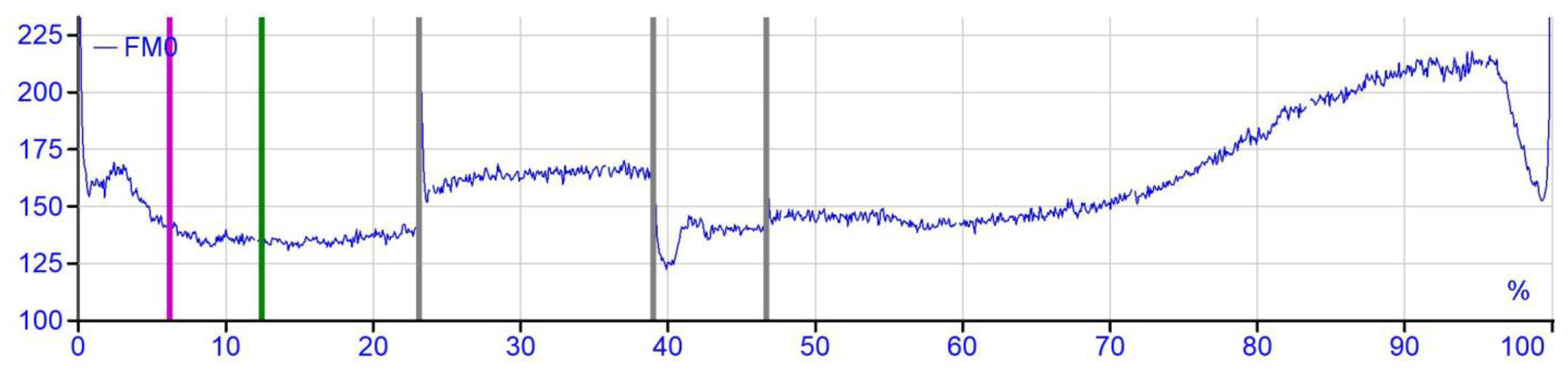
The FM0 [25] is similar to the crest factor, but instead of dividing the maximum peak value by the RMS value, the maximum peak to peak value is divided by the sum of the amplitudes of the meshing frequency harmonics. Therefore, Time Synchronous Averaging (TSA) is applied to the time signal. It is expected to obtain better results for transmission monitoring with this indicator compared with the crest factor.
3.6. Methodology
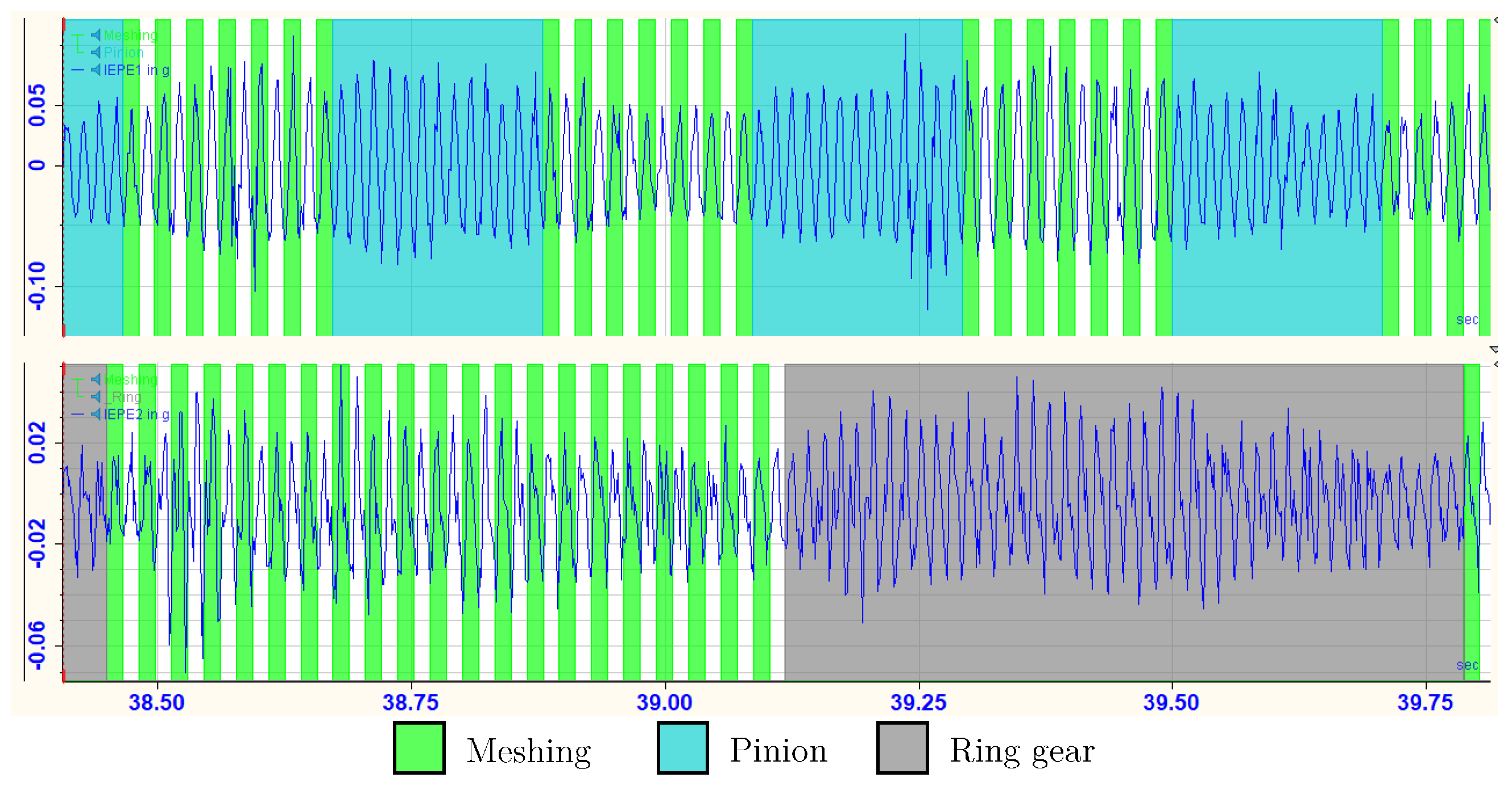
In the following section, all the signals used for damage detection are presented. The signals were resampled as described in the Section 3.3. To present the signals, an arbitrary time section from an undamaged gear is chosen. The abscissas of the diagrams shows the time in seconds. The periods of meshing and the rotation of the gears are shown with different colors on the following figures. Each coloured strip, followed by a white field, stands for one period of meshing or rotation. The legend for the colors is presented below each figure.
The raw acceleration signals in g from the two sensors, IEPE1 (upper diagram) and IEPE2 (lower diagram) are presented in Figure 7. It can be seen that the signals are very similar, with almost no noise. The amplitude modulation of the ring gear is distinguishable. The meshing frequency is also conspicuous in the signal. Considering how clearly the meshing can be seen in these signals, we can conclude that both can be used for monitoring the meshing and the damage to the gears.
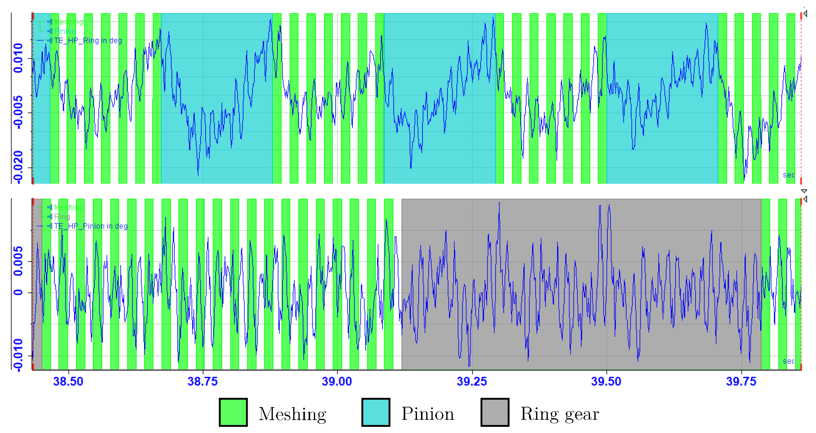
In Figure 8, the torque signal, measured at the pinion gear (), and the TE signal are depicted. The torque signal is shown in the upper part of the diagram, and it is scaled in % of rated torque. TE is presented below, in degrees, and it is calculated based on the ring gear rotation, using the Formula (13) derived from [27]. The period of the ring gear rotation (gray area) can be seen on both diagrams well. The meshing (green stripes) can be seen in the torque and TE diagrams with the calculated meshing frequency. Both diagrams show clear signals with almost no noise. The long wave component of both signals with the ring gear rotation is caused by run-out of the ring gear. This can be either radial or axial run-out. Due to the scaling of the TE, the meshing component cannot be seen well on the diagram. To be able to see the meshing frequency, the signal has been high-pass filtered both with the ring gear and the pinion gear frequency. The filtered signals are presented in Figure 9.
In the upper part of Figure 9, the frequency of the pinion gear is very distinct, together with the meshing frequency. Like in the case of the ring gear described above, this is the result of pinion gear run-out. After high-pass filtering the signal with the pinion gear speed, the frequency of the meshing can be seen more clearly. Summarizing the torque and TE signals, it can be said that due to the low level of noise and the clearness of the meshing in the signals, and it is suspected that these features can be utilized for damage detection.
4. Evaluation of Condition Indicators
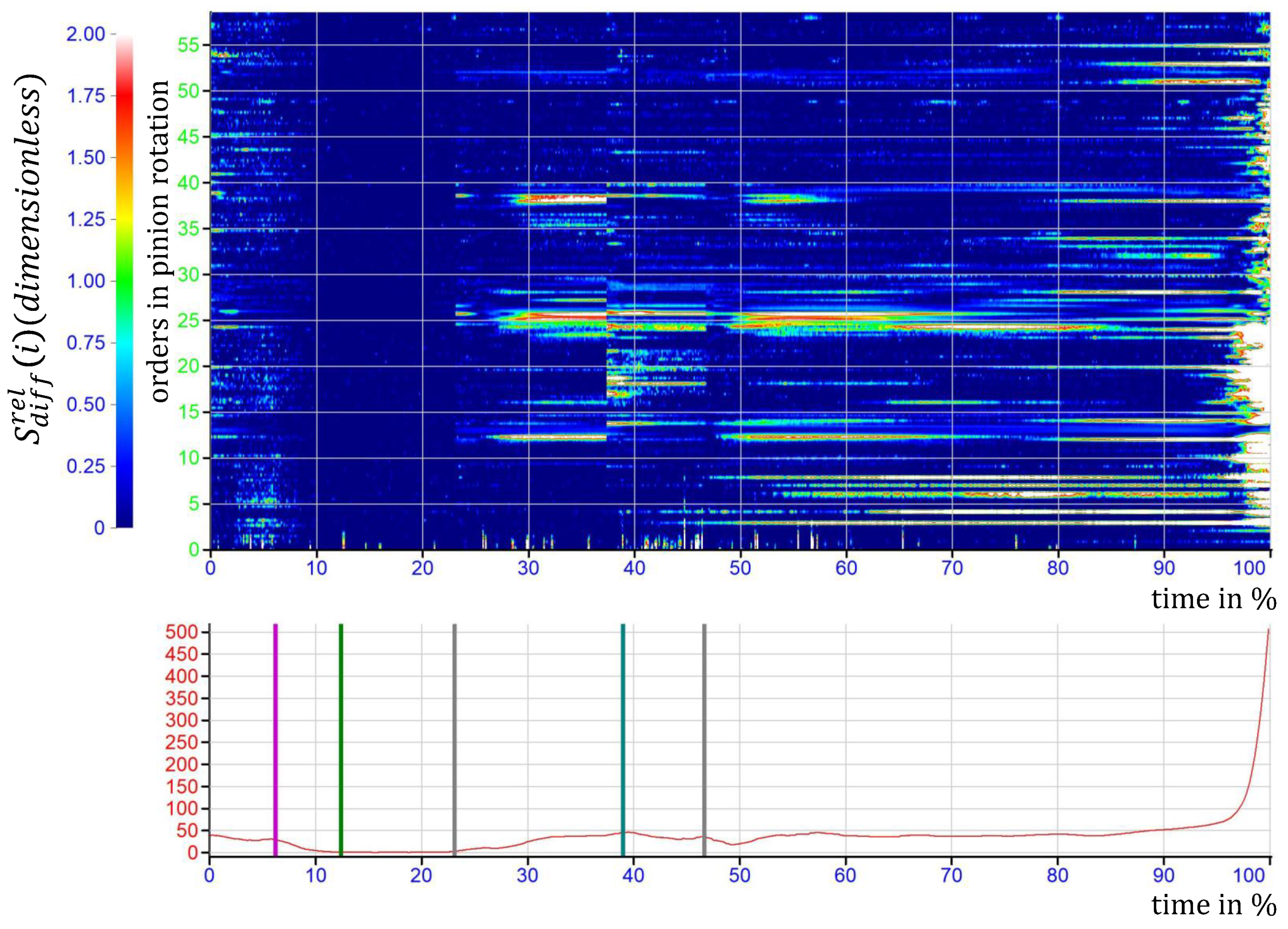
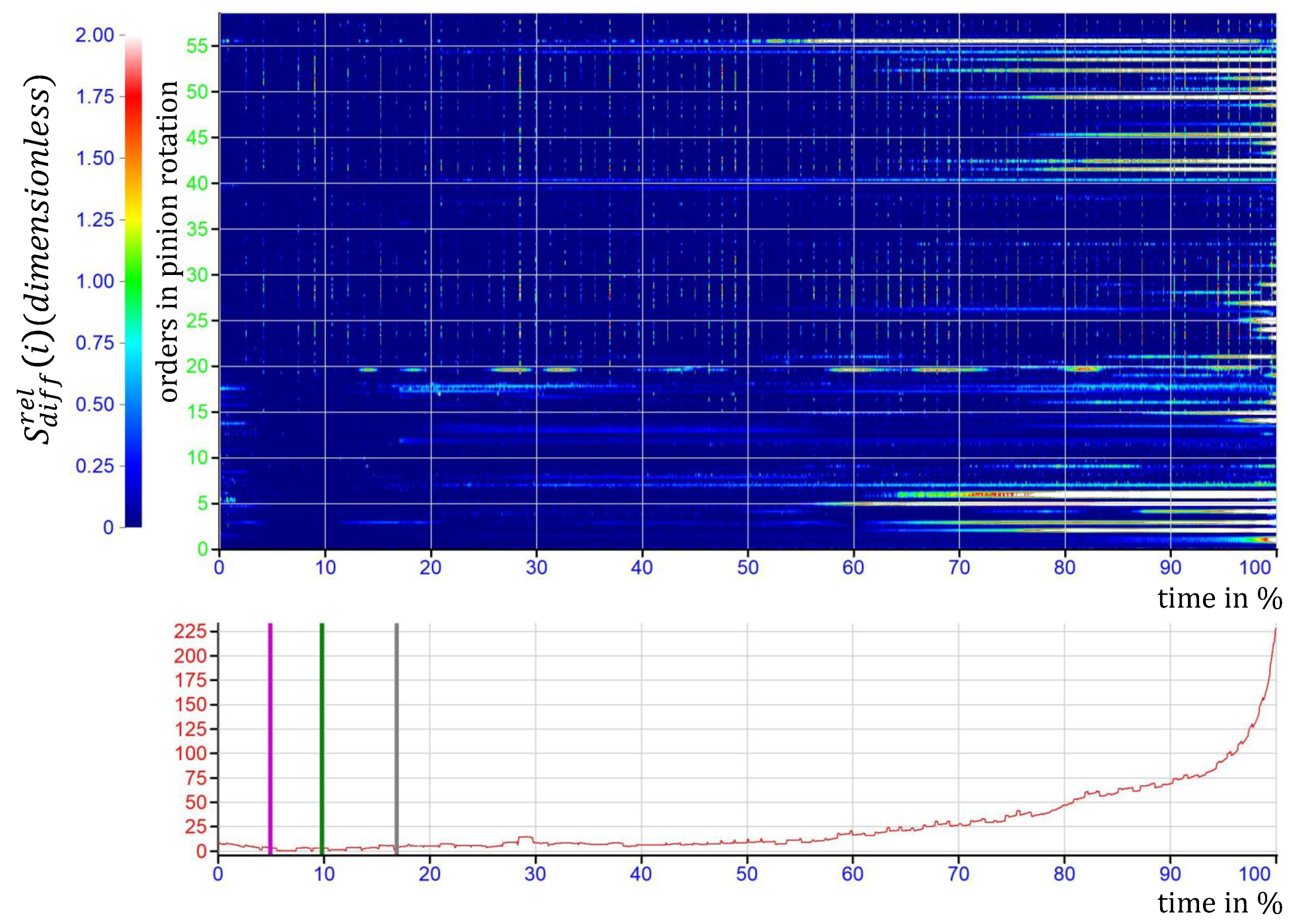
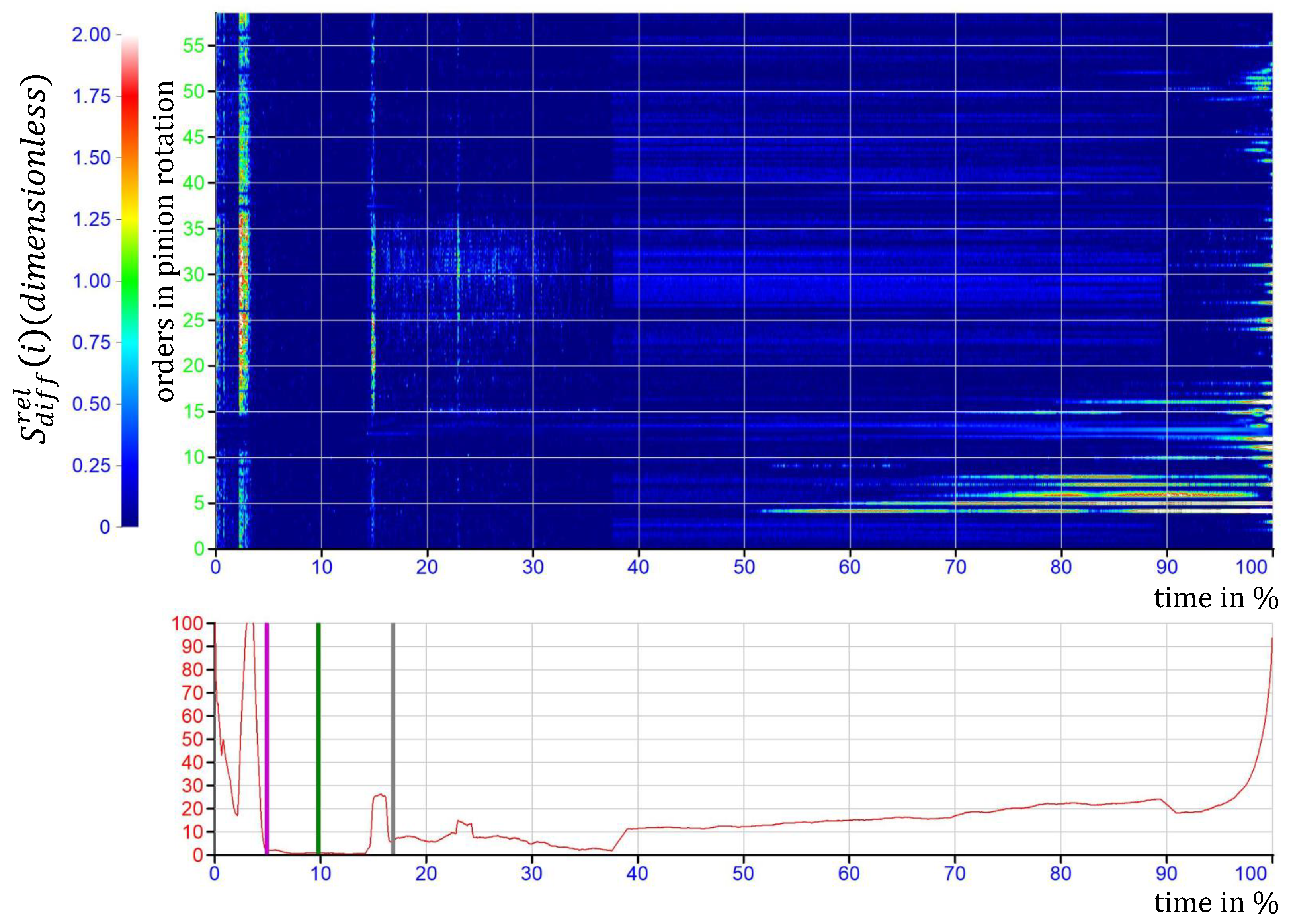
The results of the damage detection were evaluated for two exemplar samples. An overview of the samples, with the applied load and damage, can be found in Table 3. The speed of the test bed was the same for all the samples, , the speed of the pinion gear was 291 RPM, and the speed of the ring gear, was the same, with a ratio of , 89.76 RPM. The results shown as colorplots are scaled to the pinion speed, so the 1st order is equal to the rotation frequency of the pinion gear and the 13th order with the meshing frequency. The order scale is the ordinate of the colorplots. It was decided to present the on the colorplots (third dimension, colour) in order to see the influence of weaker frequency bands as well. The relative spectral difference is dimensionless and represents the relative difference to the learned value of each bin (e.g., 1.5 = 1.5 × more than learned). The abscissas of the colorplot and the trend diagram below, shows the total elapsed testing time from the start until breakage in percentage. The trend line is the of the upper colorplot and it shows dimensionless the sum of the relative spectral difference. In other words, the sum of the changes of all bins in the spectrum.
The learning period was varied widely and the results showed very low sensitivity. The selected learning length of 870 s corresponds to approx. 100 hunting tooth cycles (the period of one hunting tooth at the given speed is 8.66 s ) or 55,000 meshing cycles.
The following representation of the results shows pinion tooth bending fatigue breakage for Sample and Sample .
In the description of the results the observed orders are defined at the discrete bins of the spectrum; hence, the numbers of the orders are not round numbers. The choice was made to present the results in this way to emphasize the discrete resolution of the analysis and not to give the false impression of orders laying exactly at the characteristic frequencies of components. The only exceptions to this are a few cases where several harmonics of a gear are dominant, here the integer orders are listed to keep the description compact. In order to offer an overview in the assessment of the results, only a list of the most significant orders is given to help the interpretation of the diagrams. The purpose of the list is to show if the same orders can be systematically recognized for a certain failure mode. The time indications are given as a percentage of the testing time.
The start and end of the learning phase and the testing stops are indicated with vertical lines in the trends () with the respective colors: magenta, green and gray.
Additionally, indicators were also calculated for the TE spectra. The CIs (sideband ratio (SBR) and sideband index (SBI)) can be calculated for both gears, as the sidebands of the pinion and ring gear are spaced differently from the meshing frequency. This implies the chance of separating the damages on the gears; hence, the indicators have been calculated for the ring gear and pinion gear.
A further objective of the approach using the spectra as the input for the CIs, was to see if the CIs preform better with pre-processed and filtered information while also assessing if any advantage can be generated compared to the manual assessment of the dominant orders, also in terms of separating the damaged gear. As many spectral lines show increased activity on the colorplots, a manual assessment of the spectrum can be difficult and an automated approach may have benefits. The evaluation of the indicators can also be considered as an automated analysis of the results.
In Section 4.1, the results are only briefly summarized at the end of each section. The analysis of all results in terms of the possibility for the usage of damage detection is described in Section 6.
4.1. Test Results
On inspection, the damage to Sample was found to include the fracture and removal of one pinion tooth and the visible cracking of a neighboring tooth. The neighboring tooth was assumed to be a secondary failure as a result of the increased load share once the fully cracked tooth had weakened.
Metallurgical analysis found that the cause of the fracture on the pinion gear was tooth root bending fatigue, which had the initiation at a Non-Metalic Inclusion (NMI). The crack from the fractured surface demonstrated a “fish eye” feature, around the NMI and near the drive flank surface, while ductile failure surfaces, including wide “tidemarks”, were seen towards the tooth core. No cracks were found on the ring gear through visible inspection or with magnetic particle inspection.
In Figure 10, the results from Sample are presented, showing the colorplot and the trend of TE. It can be seen that immediately after the learning period, only the 22.82nd order shows up clearly, and some activity at the 2.63rd order and above the 25th order can be seen. These contribute only to a slight change of the trend. At approx. 23% of the lifetime of the sample, the testing was interrupted for contact pattern measurement and a new position of the samples was set up. This caused a moderate increase in the trend and some orders are also visible in the colorplot from this point. Otherwise, the trend and the colorplot stay stable until around 39% of the testing time, where a restarting of the test occurs and manifests as a peak in the spectrum and trend. From this point in time, some orders are observed in the colorplot that were not visible before, such as the 13.75th and 26.33rd orders. After a stop and restart at approx. 48% of the testing time, the trend increases linearly with slightly changing gradients until around 90% of the lifetime. At this point, a rapid increase in the trend starts, caused by the following orders (exemplary selected orders): 7.03rd, 11.12nd, 16.97th, 19.01st, 23.99th, and 24.86th. The orders between the 11.12nd and the 19.01st are smeared over, so it is not possible to find single orders contributing to the change in the trend in this area of the plot. After the rapid increase, the sample fails with a fatigue breakage removing one pinion tooth completely. The visual inspection shows that all other pinion teeth are cracked in their roots.
Figure 11 depicts the colorplot and the trend of . The development of the trend is very similar to that of the TE. The colorplot is generally also similar to the results with TE. The stop at 23% of the testing time and adjustment of the contact pattern is visible here as well, just like the restart at around 39%. The exponential increase in the trend also starts at approx. 90% of the testing time. The following list shows some of the orders causing a change in the trend: 7.9th, 12.29th, 16.97th 26.62nd, 43rd, and 54.7th.
The results of the accelerometer, named IEPE1 (ring gear side accelerometer, radially oriented), are presented in Figure 12. The bright areas on the colorplot at the beginning of the measurement, before restart from approx. 13% until 23% (restart) and after 38% of the testing time, dominate both diagrams at first sight. This phenomenon has been assessed in detail in [10]. It was found that is caused by continuous impacts from an unknown source, either related to the condition of the gears nor to the meshing. The impacts begin after starting the tests, appearing between 15% and 23% of the testing time. After the restart at 23% of lifetime, the impact reappears and fades out. The same trend can be observed after the restart at 40%, where the impacts fade out and completely disappear. After 50% of the testing time the trend increases linearly, similar to that of TE and , but with some local maximum and minimum until approx. 95%, where an rapid increase in the trend starts. Some of the dominant orders causing the rapid increase are 2.93rd, 4.97th, 5.85th, 7.9th, 13.46th, and 24.86th. On the colorplot between the 12th and 17th orders, the lines are smeared, so it is not possible to identify single orders. Furthermore, between the 36th and the 53rd orders, numerous lines of the colorplot feature increased activity.
In Figure 13, the results of the accelerometer on the pinion gear are shown. The trend and the colorplot are very similar to that of the other accelerometer. The stop of the testing at 23%, 38% and 46% of lifetime is clearly visible in the spectrum. Nevertheless, the change in the trend after restarting the test is minimal. From around 25%, the following dominant orders appear on the colorplot: 11.99th, 25.45th, and 38.03rd. Near breakage, from approx. 95%, the trend increases rapidly. With the use of the same scaling of the color axis as in other diagrams, it is not possible to identify single orders contributing to the change, as most of the orders show a change by at least 75–100%. By changing the scale the following orders are the most dominant: 2.93rd, 7.9th, 10.24th, and 21.06th.
The results calculated using the TE are depicted in Figure 14. The indicators SBR_TE_Pinion, SBR_TE_Ring and SBI_TE_Pinion are similar to the of TE (called CI_TE, on the very top of the figure). The SBR of the ring gear (called SBR_TE_Ring, fifth diagram) has a significantly different development. The absolute value of the SBR_TE_Ring is lower than the same indicator of the pinion gear. This points to the direction that the SBR, based on the can be used to detect the damaged gear, as the SBR of the pinion gear shows the damage as clearly as the CI_TE, whereas the SBR of the ring gear does not exhibit a clear exponential increase with the same magnitude.
On inspection, the damage to Sample was found to be a fatigue tooth root bending crack, which resulted in the breakage of two teeth and the cracking of a further two. The metallurgical analysis found that the cause of the failure had been a fatigue breakage, with an unknown initiation site. No cracks were found on the ring gear through visible inspection or with magnetic particle inspection.
The colorplot and trend calculated using TE, of Sample are shown in Figure 15. Similar to Sample , after the restart and re-positioning of the samples at 16% of the testing time, slight changes could be seen in the spectrum, without significant influence in the trend. The trend stays stable on a low level till around 50% of the lifetime of the sample. After this point, harmonics next to the rotational frequency appear in the spectrum, such as 2.05th, 2.93rd, 4.97th, 5.85th, 7.9th, and 14.92nd, which contribute to a linear increase in the trend. This increase continues more or less linearly till 90%, where an exponential increase in the trend is to be observed until breakage. During this rapid development of the trend, amongst others, the following orders show increased activity: rotational harmonics from the 2nd to the 7th, 14th, 14.04th, 22.82nd, and 24.86th orders.
The torque results of Sample depicted in Figure 16 are comparable with those of TE. The colorplot shows more activity in the higher frequency regions. From 50% of the testing time, as the trend starts to increase linearly, among others, the following orders become dominant: 2.05th, 2.93rd, 4.97th, 6.14th, 41.24th, 42.41st, and 55.28th. Near to the end of the test, from 90%, the 2.93rd, 4.1st, 6.14th, 14.92nd, 26.91st, 45.34th, and 52.36th orders show increased activity. This trend is similar to the trend of TE.
In Figure 17, the results calculated from the acceleration signal of IEPE1 are presented (pinion gear side accelerometer, axially oriented). As for, Sample impacts are visible both in terms of the spectrum and the trend. This broad excitation can be seen before the learning phase starts at approx. 3% of the testing time and shortly before the restart of the test at 16%. Slight impacts are also visible after restart. Except for the effect of the impacts, the trend is similar to that of the TE, but the linear increase starts earlier in time, at 40% instead of 50%, with a smaller slope and a broad activity on the spectrum between approx. the 20th and 50th orders. The exponential rising part of the graph starts after a local minimum at 95%. Here the following dominant orders can be observed: rotational harmonics from the 2nd to the 5th order, most of the rotational harmonics between the 10th and the 17th orders, the 42.12th, 50.31st, 50.84th, and 51.45th orders.
Figure 18 depicts the results of the accelerometer IEPE2. The results are only partly similar to the other parameters. The trend is different from all other above described parameters, apart from a local maximum at around 29% of the testing time. It is nearly constant from around 35% until a linear increase at approx. 80%, followed by a rapid growth from 93%. The restart of the test bed is slightly visible on the colorplot. From around 20%, the following dominant orders appear on the colorplot (it is hard to define single orders, due to the high amplitude in the proximity of the listed orders): 12.29th, 26.62nd, and 28.37th. The contribution of these orders is insignificant to the change of the trend, compared to the increase at the end of testing. Near the end of the lifetime of the sample, the following orders show increased activity: most of the rotational harmonics between the 3rd and the 25th orders, 33.93rd, 43rd, and 52.94th
Figure 19 shows the indicators calculated using the of TE; these are very similar to the results of Sample . Like in the case of Sample the SBR of the ring gear differs very much from SBR of the pinion. The former has a significantly lower level, without the exponential change at the end of the testing. This also indicates in the case of Sample that the determination of the damaged gear is possible with this indicator. All other indicators are similar to of TE and cannot be used to determine which gear is damaged.
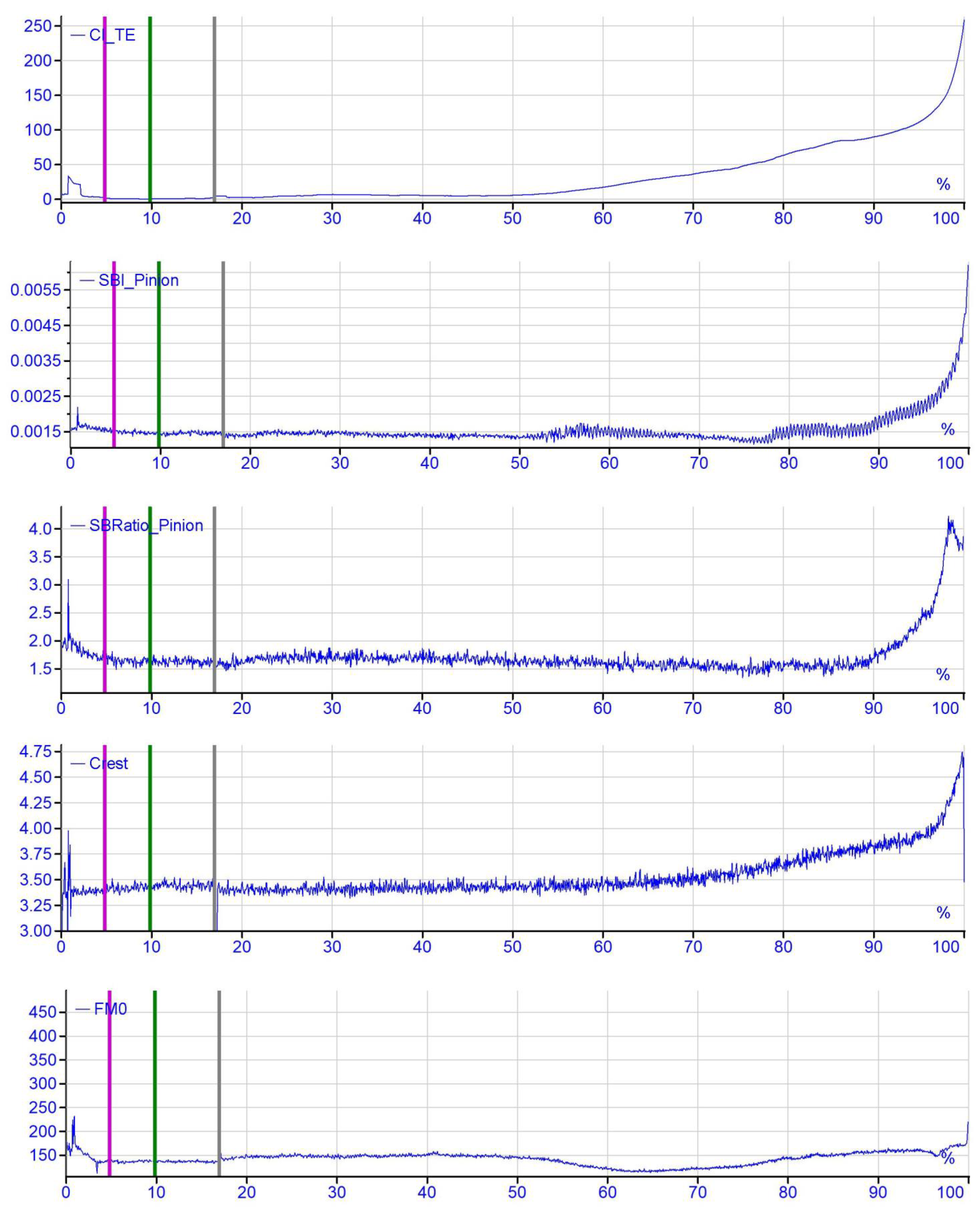
4.2. Results with Alternative Condition Indicators
The figures displaying the results with other CIs can be found for Sample in Figure 20 (pinion gear), Figure 21 (ring gear) and for Sample in Figure 22 (pinion gear), Figure 23 (ring gear). In the following comparison, the indicators are compared with the of TE (presented as on the top of each diagram) as this trend is considered to be usable for the damage detection. The indicators based on the ring gear orders are also calculated and evaluated; this is also the case if the main damage occurred for both samples on the pinion gear. The goal of this is to see if the determination of the damaged gear can give an overview of all the results.
The SBIs of both samples and both gears are similar to the , whereas unlike the , the SBIs of the ring gears has some local maxima near the restart of the test bed and unlike the SBIs of the pinion gears, the trend fluctuates more. This makes the SBI ring gear less ideal for stopping the test bed in case of damage. The SBR of the pinion is very similar for both samples, showing a clear peak near to the breakage, followed by a decrease in the curve. To be able to conclude if the peak in the trend has some connection to the damage to the gears, more testing is needed to draw full conclusions. The SBR of the ring gear is similar to the SBR of the pinion gear in the case of Sample , whereas the SBR of the ring gear of Sample is different from the same indicator of the pinion gear, with a significantly flatter progress. It can be said that for these two samples that the SBR of the ring gear could not be used for both samples for damage detection. The crest factor and FM0 are not similar to the trend of , offering very little information on the samples. The only possible indication of damage can be seen in the crest factor of Sample , as it increases quickly near to the damage.
Summarizing the comparison, many alternative indicators can be used well compared to the of TE. SBI shows the damage consistently for both samples, on the pinion and ring gear, although the determination of the damaged gear is not possible with any of the indicators. It is interesting to note that some indicators show damage on the ring gear (SBI, SBR), whereas during the test the pinion gear was damaged.
5. Discussion
Summarizing the results for Sample , it can be stated that the trend of TE and show the breakage equally well, with a relatively clean spectrum. The most dominant orders are harmonics or close to the harmonics of the rotation frequency. The torque spectrum shows more activity in the high-frequency range. The trends and colorplots of the accelerometers forecast the damage a bit later in time than TE and . The spectrum shows, in the case of acceleration, more variation due to the restarting of the test bed, but these signals could be used to stop testing before breakage occurs as well. Dominant orders are also harmonics of the rotation speed in the case of acceleration spectra. Using the trends of SBR_TE_Pinion and SBR_TE_Ring, based on , it is possible to differentiate between the damaged gear, and it is apparent from these trends that the pinion gear is damaged.
Recapping the results of Sample , it is apparent that stopping the test before the breakage of the tooth occurs is possible with the use of the algorithm, with any of the parameters considered. As for Sample , using the trend of TE and the torque, an earlier stop could have been achieved compared to using the acceleration signals. It is true for all of the parameters that the most dominant orders are harmonics or close to the harmonics of the rotation frequency. The spectrum of the torque also shows more activity for this sample in the higher-frequency regions than the TE spectrum.
Considering the damage of Sample , two broken pinion teeth, it is not possible to find any indication to the event of the breakage of a single tooth using the above presented results. However, with more testing of the gears and the CI, it may be possible to relate the actual damage more effectively to the results. The determination of the damaged gear is possible for this sample as well, using the SBR, calculated from the of TE.
Based on the key performance indicators of signal-to-noise ratio, sensitivity, differentiation of damaged sample and detection time within the sample lifetime, the CIs can be contrasted. The results of this comparison have been summarized in Table 4.
To fully explore and assess the capabilities of the CI and the described method, it is necessary to extend the research work to more samples, different types of gears and also to other types of machine parts.
6. Conclusions
It has been shown for the analyzed samples that the failures are visible in the trend () and colorplot () of all measured signals. With slight time differences in the possibility to determine when the initial failure occurs, all signals considered can be used for this purpose. In addition to demonstrating the strength of the proposed CI, it has been shown that the torque signals can also be used for condition monitoring, in addition to the well known acceleration and TE signals, offering possibilities for wide application of the CI and faster processing.
In comparison of the proposed CI to other well known indicators, the only indicator which was similar to the and could indicate the damage in all cases was the SBI. The SBR showed a different trend from the , but it could be used for damage detection. The crest factor and the FM0 did not produce comparable results to the in any case, and could not consistently indicate the damage. It can be concluded that to determine the gear damage in the shown case, the evaluation of the complete spectrum with the does not offer a benefit over the SBI, which only monitors gear rotational and meshing harmonics.
It has been shown that with the usage of SBR as post-processing of the TE, the determination of the damaged gear is also possible in the case of pinion damage. This indicator is also capable of showing which one of the gears was damaged. This approach should be assessed in the future with more samples and varied test conditions to see if it can be consistently used to determine the damaged gear.
In the testing considered here, the failure modes observed did not allow enough variation to make a significant conclusion on the proposed CI ability to identify between the route causes of the failures. By tracking the variation in the spectrum, it would be possible to identify which frequencies display a disparity and from this determine the likely cause of failure.
It was observed that in the case of TE in the presented cases it is sufficient to monitor and evaluate the spectrum until approx. the 33rd order of the pinion gear (slightly below the third harmonic of the meshing frequency). All other signals showed activity in the complete spectrum, so the recommendation to monitor the frequencies until the fourth harmonic of the meshing frequency, as discussed in the Section 3.3, was useful and this approach delivers acceptable results. However, approaches evaluating more or less spectral lines were not assessed in this study.
Additionally, as presented in Table 4 the is the only indicator with which it is possible to detect the damage of the pinion gear and which can be potentially used for the monitoring of other components than gears. Furthermore, as shown in the comparison with other indicators in [23], the can also be used for the ultra-low -speed monitoring of planetary gears, where the other algorithms fail to detect the damage.
Author Contributions
Conceptualization, M.S. and M.L.; methodology, M.S., M.L. and C.R.; formal analysis, M.S.; investigation, M.S., M.L. and M.B.; data curation, M.S.; writing—original draft preparation, M.S., M.L. and C.R.; writing—review and editing, M.B. All authors have read and agreed to the published version of the manuscript.
Funding
Open Access Funding by the Graz University of Technology.
Institutional Review Board Statement
Not applicable.
Informed Consent Statement
Not applicable.
Data Availability Statement
Not applicable.
Acknowledgments
This research was supported by AVL List GmbH and the authors would like to thank them for their technical support in testing.
Conflicts of Interest
The authors declare no conflict of interest.
References
- Ford, J. Machine Downtime Costs UK Manufacturers £180bn a Year. The Engineer, 13 November 2017. [Google Scholar]
- Williamson, J. Downtime Costs UK Manufacturers £180bn a Year. The Manufacturer, 17 November 2017. [Google Scholar]
- Mobley, R.K. An Introduction to Predictive Maintenance; Elsevier: Amsterdam, The Netherlands, 2002. [Google Scholar] [CrossRef]
- Einabadi, B.; Baboli, A.; Ebrahimi, M. Dynamic Predictive Maintenance in industry 4.0 based on real time information: Case study in automotive industries. IFAC-PapersOnLine 2019, 52, 1069–1074. [Google Scholar] [CrossRef]
- Ahmad, R.; Kamaruddin, S. An overview of time-based and condition-based maintenance in industrial application. Comput. Ind. Eng. 2012, 63, 135–149. [Google Scholar] [CrossRef]
- Curcurù, G.; Galante, G.; Lombardo, A. A predictive maintenance policy with imperfect monitoring. Reliab. Eng. Syst. Saf. 2010, 95, 989–997. [Google Scholar] [CrossRef]
- Nandi, A.; Ahmed, H. Condition Monitoring with Vibration Signals; John Wiley & Sons.: Hoboken, NJ, USA, 2019. [Google Scholar] [CrossRef]
- Rao, B. Handbook of Condition Monitoring; Elsevier: Amsterdam, The Netherlands, 1996. [Google Scholar]
- Randall, R.B. Vibration-Based Condition Monitoring; John Wiley and Sons, Ltd.: Hoboken, NJ, USA, 2011. [Google Scholar]
- Surányi, M. Condition Monitoring Methods for Powertrain Test Beds. Ph.D. Thesis, Institute of Machine Components and Methods of Development, Technical University Graz, Graz, Austria, 2021. [Google Scholar]
- The Japanese Society for Non-Destructive. Practical Acoustic Emission Testing; Springer: Tokyo, Japan, 2016. [Google Scholar]
- Loutas, T.H.; Sotiriades, G.; Kalaitzoglou, I.; Kostopoulos, V. Condition monitoring of a single-stage gearbox with artificially induced gear cracks utilizing on-line vibration and acoustic emission measurements. Appl. Acoust. 2009, 70, 1148–1159. [Google Scholar] [CrossRef]
- Scheer, C.; Reimche, W.; Bach, F.W. Early Fault Detection at Gear Units by Acoustic Emission and Wavelet Analysis. J. Acoust. Emiss. 2007, 25, 331–340. [Google Scholar]
- Mark, W.D. Performance-Based Gear Metrology; Wiley Online Library: Hoboken, NJ, USA, 2012. [Google Scholar]
- Hu, C.; Smith, W.A.; Randall, R.B.; Peng, Z. Development of a gear vibration indicator and its application in gear wear monitoring. Mech. Syst. Signal Process. 2016, 76, 319–336. [Google Scholar] [CrossRef]
- Loutridis, S.J. Damage detection in gear systems using empirical mode decomposition. Eng. Struct. 2004, 26, 1833–1841. [Google Scholar] [CrossRef]
- Endo, H.; Randall, R.B.; Gosselin, C. Differential diagnosis of spall vs. cracks in the gear tooth fillet region: Experimental validation. Mech. Syst. Signal Process. 2009, 23, 636–651. [Google Scholar] [CrossRef]
- Mark, W.D.; Isaacson, A.C.; Wagner, M.E. Transmission-error frequency-domain-behavior of failing gears. Mech. Syst. Signal Process. 2019, 115, 102–119. [Google Scholar] [CrossRef]
- Klingelnberg, J. Bevel Gear; Springer: Berlin/Heidelberg, Germany, 2016. [Google Scholar]
- Schlecht, B. Maschinenelemente 2; Ing. Maschinenbau, Pearson Studium: Cham, Switzerland, 2010. [Google Scholar]
- Braunstingl, M. Advanced Gear Optimization for AWD Systems. Available online: https://eawdcongress.com/download/braunstingl.pdf (accessed on 3 December 2012).
- Mark, W.D.; Lee, H.; Patrick, R.; Coker, J.D. A simple frequency-domain algorithm for early detection of damaged gear teeth. Mech. Syst. Signal Process. 2010, 24, 2807–2823. [Google Scholar] [CrossRef]
- Surányi, M.; Reinbrecht, C.; Huemer, H. Experimental study of failing differential gears and introduction of a new condition indicator for ultra low speed applications. Mech. Syst. Signal Process. 2021, 155, 107588. [Google Scholar] [CrossRef]
- Klein, U. Schwingungsdiagnostische Beurteilung von Maschinen und Anlagen, 3rd ed.; Verl. Stahleisen: Düsseldorf, Germany, 2003. [Google Scholar]
- Večeř, P.; Kreidl, M.; Šmíd, R. Condition indicators for gearbox condition monitoring systems. Acta Polytech. 2005, 45, 35–43. [Google Scholar] [CrossRef]
- Stewart, R. Some Useful Data Analysis Techniques for Gearbox Diagnostics. Machine Health Monitoring Group Report MHM; Technical Report, R/10/77; University of Southampton: Southampton, UK, 1977. [Google Scholar]
- Bassett, D.E.; Houser, D.R. The Design and Analysis of Single Flank Transmission Error Tester for Loaded Gears; Technical Report; Ohio State Univ. Columbus Dept. of Mechanical Engineering: Columbus, OH, USA, 1987. [Google Scholar]
Figure 1.
Definition of hypoid offset.

Figure 2.
Definition of E, P, G, [21].
Figure 2.
Definition of E, P, G, [21].

Figure 3.
Specialized gear rig.

Figure 4.
Test bed structure and control.

Figure 5.
Additional sensors for CM.

Figure 6.
Application of the CI to a procedure with multiple operating points, using ID labels to monitor effectively.
Figure 6.
Application of the CI to a procedure with multiple operating points, using ID labels to monitor effectively.

Figure 7.
Raw acceleration signals in g vs. time in seconds.

Figure 8.
Upper diagram: Raw torque signal in % of rated torque vs. time in seconds. Lower diagram: TE signal in degree vs. time in seconds.
Figure 8.
Upper diagram: Raw torque signal in % of rated torque vs. time in seconds. Lower diagram: TE signal in degree vs. time in seconds.

Figure 9.
High-pass filtered transmission error signals in degree vs. time in seconds. Upper diagram: filtered with ring gear frequency. Lower diagram: filtered with pinion gear frequency.
Figure 9.
High-pass filtered transmission error signals in degree vs. time in seconds. Upper diagram: filtered with ring gear frequency. Lower diagram: filtered with pinion gear frequency.

Figure 10.
Colorplot and trend of TE of Sample .

Figure 11.
Colorplot and trend of M of Sample .

Figure 12.
Colorplot and trend of the accelerometer IEPE1 (ring gear) of Sample .

Figure 13.
Colorplot and trend of the accelerometer IEPE2 (pinion gear) of Sample .

Figure 14.
Alternative indicators calculated with TE 200 bands for Sample pinion and ring gear orders.
Figure 14.
Alternative indicators calculated with TE 200 bands for Sample pinion and ring gear orders.

Figure 15.
Colorplot and trend of TE of Sample .

Figure 16.
Colorplot and trend of M of Sample .

Figure 17.
Colorplot and trend of the accelerometer IEPE1 (ring gear) of Sample .

Figure 18.
Colorplot and trend of the accelerometer IEPE2 (pinion gear) of Sample .

Figure 19.
Alternative indicators calculated with TE 200 bands for Sample pinion and ring gear orders.
Figure 19.
Alternative indicators calculated with TE 200 bands for Sample pinion and ring gear orders.


Figure 20.
Alternative indicators calculated with TE 200 bands for Sample pinion orders.


Figure 21.
Alternative indicators calculated with TE 200 bands for Sample ring orders.

Figure 22.
Alternative indicators calculated with TE 200 bands for Sample pinion orders.

Figure 23.
Alternative indicators calculated with TE 200 bands for Sample ring orders.


Table 1.
Overview of the used sensors for CM.
| Sensor Name | Type |
|---|---|
| Accelerometer | PCB M608A11 |
| Torque transducer | HBM T12HP rated at 5 and 10 kNm |
| Rotation speed | INC-4-225-191001-ABZ2-RFC3-24-AN |
Table 2.
FFT settings.
| Parameter | Setting |
|---|---|
| sampling frequency | 730 Hz |
| number of samples | 4096 |
| 285.15Hz | |
| 0.178 Hz | |
| overlap | 0% |
| update time | 5.61 s |
| averaging | None |
| suppress DC | True() |
| detrend raw data | True() |
| windowing | Hanning |
| normalized | False() |
| spectrum method | magnitude |
Table 3.
Overview of the tests.
| Sample | Testing Time | in Sec | in Sec | Observed Damage | |
|---|---|---|---|---|---|
| Sample | 1.3 × rated torque | Approx. 4 h | 870 | 870 | light spalling and tooth bending fatigue cracks on the pinion |
| Sample | 1.3 × rated torque | Approx. 5 h | 870 | 870 | light spalling and tooth bending fatigue cracks on the pinion |
Table 4.
Summary of the results and comparison of the tested indicators.
| Sample AH | Sample BH | ||||||||
|---|---|---|---|---|---|---|---|---|---|
| SNR | Sensitivity | Differentiation between Failed Gear | Detection Time | SNR | Sensitivity | Differentiation between Failed Gear | Detection Time | Monitoring Other Components than Gears | |
| RSDabs | good | exponential change | no | 90% | good | exponential change | no | 90% | yes |
| SBI_Pinion | good | exponential change | no | 90% | good | exponential change | no | 90% | no |
| SBI_Ring | good | linear change | 90% | good | exponential change | 88% | |||
| SBI_TE_ Pinion | good | exponential change | no | 90% | good | exponential change | no | 95% | no |
| SBI_TE_ Ring | good | exponential change | 90% | good | exponential change | 90% | |||
| SBR_ Pinion | good | exponential change and drop | no | 90% | good | exponential change | maybe, as the sensitivity is different | 90% | no |
| SBR_Ring | good | exponential change and drop | 90% | average | linear change | 88% | |||
| SBR_TE_ Pinion | good | exponential change | yes | 90% | good | exponential change | yes | 90% | no |
| SBR_TE_ Ring | good | slight exponential change and drop | - | good | linear drop and increase | - | |||
| Crest | good | continuous linear change | no | - | good | linear increase | no | 95% | yes |
| FM0 | good | drop and increase at the end of testing | no | - | good | no visible trend | no | - | no |
Publisher’s Note: MDPI stays neutral with regard to jurisdictional claims in published maps and institutional affiliations. |
© 2021 by the authors. Licensee MDPI, Basel, Switzerland. This article is an open access article distributed under the terms and conditions of the Creative Commons Attribution (CC BY) license (https://creativecommons.org/licenses/by/4.0/).
Share and Cite
MDPI and ACS Style
Surányi, M.; Leighton, M.; Reinbrecht, C.; Bader, M. Evaluation of a Novel Condition Indicator with Comparative Application to Hypoid Gear Failures. Appl. Sci. 2021, 11, 11499. https://0-doi-org.brum.beds.ac.uk/10.3390/app112311499
AMA Style
Surányi M, Leighton M, Reinbrecht C, Bader M. Evaluation of a Novel Condition Indicator with Comparative Application to Hypoid Gear Failures. Applied Sciences. 2021; 11(23):11499. https://0-doi-org.brum.beds.ac.uk/10.3390/app112311499
Chicago/Turabian StyleSurányi, Marcell, Michael Leighton, Christian Reinbrecht, and Michael Bader. 2021. "Evaluation of a Novel Condition Indicator with Comparative Application to Hypoid Gear Failures" Applied Sciences 11, no. 23: 11499. https://0-doi-org.brum.beds.ac.uk/10.3390/app112311499
Note that from the first issue of 2016, this journal uses article numbers instead of page numbers. See further details here.