Research of Calibration Method for Industrial Robot Based on Error Model of Position

Abstract

Based on the current situation of high precision and comparatively low APA (absolute positioning accuracy) in industrial robots, a calibration method to enhance the APA of industrial robots is proposed. In view of the “hidden” characteristics of the RBCS (robot base coordinate system) and the FCS (flange coordinate system) in the measurement process, a comparatively general measurement and calibration method of the RBCS and the FCS is proposed, and the source of the robot terminal position error is classified into three aspects: positioning error of industrial RBCS, kinematics parameter error of manipulator, and positioning error of industrial robot end FCS. The robot position error model is established, and the relation equation of the robot end position error and the industrial robot model parameter error is deduced. By solving the equation, the parameter error identification and the supplementary results are obtained, and the method of compensating the error by using the robot joint angle is realized. The Leica laser tracker is used to verify the calibration method on ABB IRB120 industrial robot. The experimental results show that the calibration method can effectively enhance the APA of the robot.

1. Introduction

With the wide application of industrial robot, people have higher requirements for its positioning accuracy. However, due to the influence of manufacturing error, assembly error, joint abrasion, and transmission error of robot parts, the positioning accuracy of robot is not satisfactory, which limits the application of robot in high-precision field. Therefore, it is particularly important to study the positioning accuracy improvement method of industrial robot.

In fact, the positioning accuracy of industrial robots can be divided into two parts: repeated positioning accuracy and absolute positioning accuracy (APA) [1]. In most cases, we only need to improve the repeated positioning accuracy of the robot. For example, when industrial robot welds a workpiece, the repeated accuracy of the robot normally determines the trajectory accuracy of the workpiece directly. At this time, the APA is meaningless. Therefore, people focus on how to improve the repeat positioning accuracy, which can be improved by many methods such as soft computing and machine learning [2,3]. Industrial robots normally have the merit of high repeat positioning accuracy. For some small industrial robots, its repeat positioning accuracy even reach 0.01 mm, while the APA of the robots may be beyond 1mm or worse [4]. So in this field, the research on APA is obviously insufficient. For example, in the application of multi robot cooperation, for kinematics parameter identification and robot off-line programming tasks, it is necessary to calibrate the precise pose of the robot base coordinate frames in the world coordinate system, which requires that the industrial robot must have sufficient APA [5].

The fundamental reason for the low APA of industrial robot is that the pose of TCP (Tool Center Point) are calculated by kinematics mathematical model which contains the structure size of the linkage and motion parameters of joint. Moreover, there are errors between the values taken in calculation and actual parameters of the robot, resulting in a deviation between the calculated results and the actual pose. The following two methods can be used to enhance the robot’s APA: (1) using high accuracy machining equipment and advanced assembly method to reduce robot link machining and assembly errors; (2) combining advanced measurement tools and related algorithms to identify and correct robot structural parameters, that is robot calibration method [6]. The first method is expensive and has limited effect on improving the precision of the robot, and it cannot solve the problem of precision decline caused by wear and deformation. The second method is cheaper than first one, and it is more effective in compensating the precision degradation caused by wear or structural deformation [7]. Therefore, robot calibration is the main method to enhance the APA of robot, and it is also the main research direction of many scholars [8].

In the study of robot calibration method, Knasinski et al. [6] found that the absolute positioning error is mainly caused by the parameter error of robot kinematics model. Therefore, the research of robot calibration technology focuses on the error identification of robot kinematics parameters primarily [9,10,11]. In the current research on the reduction of APA caused by kinematic parameter errors, it usually assumes that the robot base coordinate system (RBCS) and the flange coordinate system (FCS) are known or can be directly measured. However, the fact is that most of the robot flange and base coordinate system are “hidden”—it cannot be directly measured and need to be obtained through special measurement and calculation methods [12].

In reference [13], the position and pose measurement of robot is realized by using coordinate theodolite, and the APA error of the robot is reduced to 0.28 mm after calibration. This instrument is designed according to the principle of angle detecting, and exhibits good measurement accuracy. However, the user needs to have relevant measurement skills, and the measurement results are easy to be interfered by environmental factors. In reference [14], the robot of IRB2400 was calibrated with a laser tracker. In this application, the base coordinate was obtained by means of making axis 1 and axis 2 rotate, respectively, and measuring the base plane, so that the coordinate transformation can be realized between laser tracker and robot base. Reference [15] uses the FARO ARM to calibrate the robot and obtain the RBCS by quaternion form. Nubiola [16] used Faro laser tracker to measure and calibrate ABB IRB1600 (ABB, Zurich, Switzerland) industrial robot from Switzerland. The mean absolute positioning accuracy can be reduced from 0.981 mm to 0.292 mm in eight different measurement points on the robot end effector. The measurement of the equipment is very accurate, and it can further cooperate with other relevant tools to obtain the target attitude. The equipment is easy to operate, but it is very expensive.

In addition to use the above measuring instruments to directly measure the absolute pose of the end of the robot for calibration, some scholars have studied the robot self-calibration method of indirectly measuring the pose of the end of the robot through the algorithm without relying on the measuring instruments. Beenett [17] proposed a closed-loop self-calibration method, which kept the end of the robot at a point unchanged, and changed the pose of the end of robot, so as to finally solve the closed-loop equation. Joubair [18] used multi-plane constraints to calibrate the six axes flexible robot. Legnani [19] used corded sensor to measure the position and pose of the robot and complete the calibration of the kinematic parameters of the robot.

However, in the existing robot calibration and measurement process, the pose errors of the robot caused by base coordinate system and FCS are neglected basically, which is also an important part of the robot pose error model and should be considered in the process of robot calibration, and this part of the error cannot be improved only depending on optimizing the motion algorithm of the manipulator. The absolute positioning error must be measured by a measuring instrument and then improved by the algorithm.

The robot’s calibration can be achieved by establishing the robot’s position error model or pose error model. Since most measuring devices can measure the position of the end of the robot, the position error model is more suitable for a wide range of measuring devices (such as coordinate measuring machine, six or seven axes measuring arm, laser tracker (with a target ball)). It is more versatile. This paper aims to enhance the APA of the robot. The measurement hidden errors from the robot’s flange and base coordinates and the kinematics model parameters errors are unified as the source of the absolute positioning errors. A comparatively general measurement method of robot calibration is proposed, and the algorithms of parameter error identification and compensation are discussed in detail. The algorithms are verified by experiments.

2. Robot Calibration Modeling

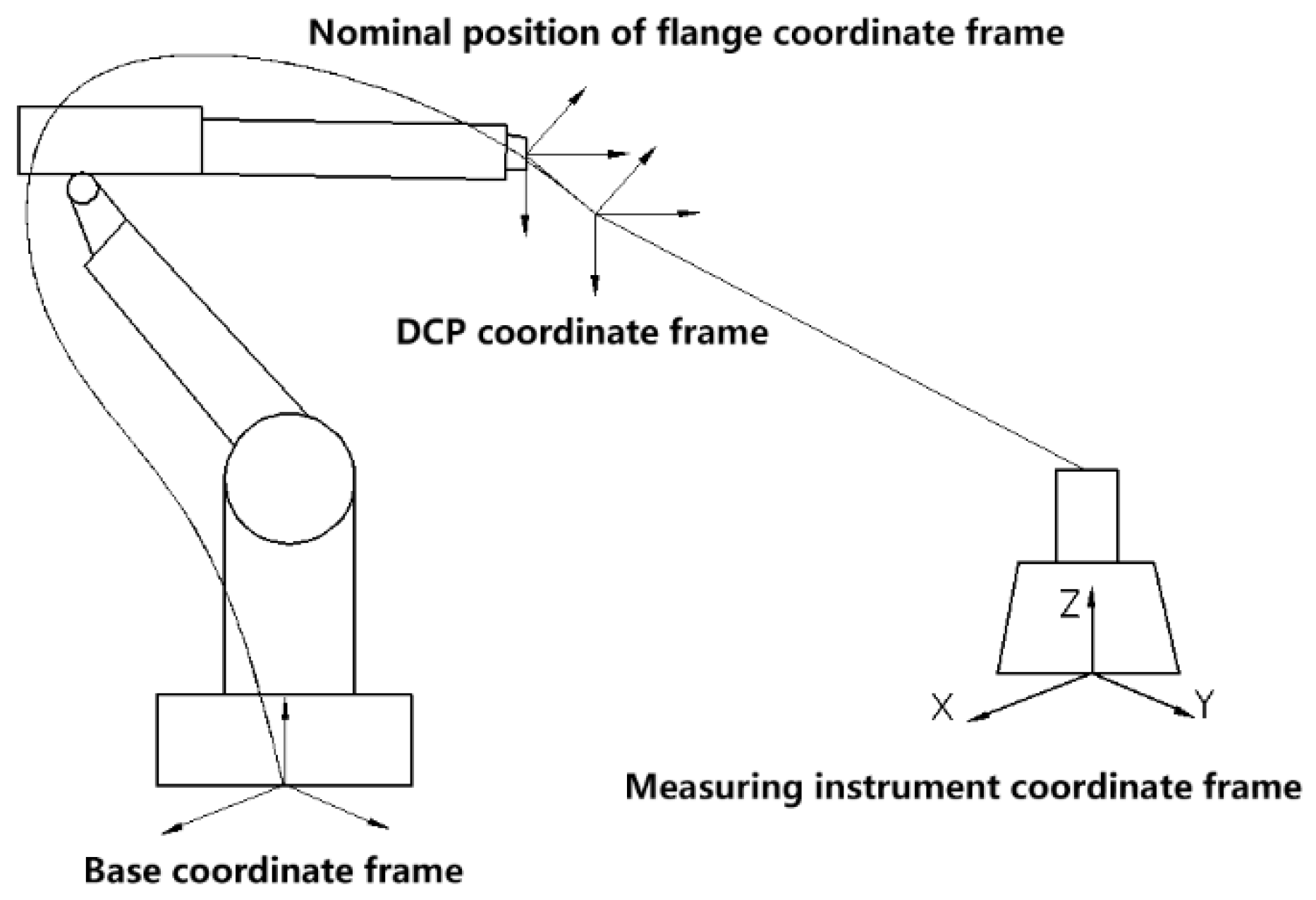
Robot calibration needs to obtain the robot end pose error in the RBCS by means of measurement. However, the actual FCS and RBCS cannot be obtained through direct measurement. Therefore, it need to establish a measurement coordinate system directly related to the measurement results. In this paper, the measured position of the measuring instrument is defined as DCP (Detection Center Point), and establishing a measurement coordinate system with DCP as the origin. When measuring the pose of the end of the robot, it is necessary to obtain the position transformation between the DCP coordinate system and FCS, and between the RBCS and MICS (measuring instrument coordinate system), so that the pose model of the DCP coordinate system in the MICS can be obtained, as expressed in Figure 1. The first step of calibration is to build a robot kinematics model that can reflect the characteristics of the end of the robot.

2.1. Robot Kinematics Modeling

The most common kinematics model of industrial robots is the four-parameter DH model (short for Denavit–Hartenberg model) proposed by Denavit [20] et al. in 1955. This model has good generality and is currently the most widely used. However, in practice, it is found that when two adjacent axes are nominally parallel, the small deviation of their mutual joint will lead to the numerical distortion in the process of parameter identification based on DH model that means the parameters are discontinuous. To avoid this problem, Hayati [21] proposes the MDH model—a modified DH model, which adds a rotational parameter to the Y axis and becomes a five-parameter model with two translations and three rotations.

$$\begin{array}{ll}{}_{i-1}{}^{i}T& =Rot(z_{i-1},{\theta }_i)·Tran(z_{i-1},d_i)·Tran(x_i,a_i)·Rot(x_i,{\alpha }_i)·Rot({\mathrm{y}}_i,{\beta }_i)\\ & =\left(\begin{array}{cccc}c{\theta }_{i}c{\beta }_i-s{\theta }_{i}s{\alpha }_{i}s{\beta }_i& -s{\theta }_{i}c{\alpha }_i& c{\theta }_{i}s{\beta }_i+s{\theta }_{i}s{\alpha }_{i}c{\beta }_i& a_{i}c{\theta }_i\\ s{\theta }_{i}c{\beta }_i-c{\theta }_{i}s{\alpha }_{i}s{\beta }_i& c{\theta }_{i}c{\alpha }_i& s{\theta }_{i}s{\beta }_i-c{\theta }_{i}s{\alpha }_{i}c{\beta }_i& a_{i}s{\theta }_i\\ -c{\alpha }_{i}s{\beta }_i& s{\alpha }_i& c{\alpha }_{i}c{\beta }_i& d_i\\ 0& 0& 0& 1\end{array}\right)\end{array}$$

(1)

In the equation, ${\theta }_i$, $d_i$, $a_i$ and ${\alpha }_i$ respectively represent the joint Angle, joint bias, length, and torsion angle of link i. In the case that joint ${\beta }_i$ exists only when adjacent axes are parallel, in other cases ${\beta }_i=0$ is directly substituted into Equation (1).

According to Equation (1), the kinematic model of a general N degrees of freedom robot can be obtained as

$${}_0{}^{N}T={}_0{}^{1}T{}_1{}^{2}T\cdots {}_{N-1}{}^{N}T=\left(\begin{array}{cccc}{n}_x& o_x& a_x& p_x\\ n_y& o_y& a_y& p_y\\ n_z& o_z& a_z& p_z\\ 0& 0& 0& 1\end{array}\right).$$

(2)

2.2. Robot Flange Coordinate Calibration Model

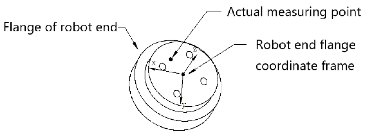
The key step of robot calibration is to obtain the actual pose error of robot end by measuring. However, the FCS of robot end is usually “hidden”, that is, it cannot be directly measured by measuring equipment [22]. There is a certain offset of the actual measured position with respect to the FCS (as expressed in Figure 2).

Let ${}_6{}^{D}T$ denote the transformation from robot FCS to DCP coordinate system. If the pose is neglected, it can be expressed as follows:

$${}_6{}^{D}T=\left(\begin{array}{cccc}1& 0& 0& P_x{}^L\\ 0& 1& 0& P_y{}^L\\ 0& 0& 1& P_z{}^L\\ 0& 0& 0& 1\end{array}\right).$$

(3)

Assuming that the FCS position of the robot is O in a certain state, when the position of the robot’s end remains unchanged, the position coordinates of O point can be obtained by fitting the center of the sphere through only changing the pose of the robot. The spherical center coordinate can be obtained by fitting more than four non coplanar points in space. Suppose the spherical center coordinates are $(a{,}_{}b{,}_{}c)$, radius is R, and the coordinates of the four measuring points are $(x_1,y_1,z_1),(x_2,y_2,z_2),(x_3,y_3,z_3),(x_4,y_4,z_4)$, respectively. The following equations can be obtained from the function expression of the sphere:

$$\{\begin{array}{c}{(x_1-a)}^2+{(y_1-b)}^2+{(z_1-c)}^2=R^2\\ {(x_2-a)}^2+{(y_2-b)}^2+{(z_2-c)}^2=R^2\\ {(x_3-a)}^2+{(y_3-b)}^2+{(z_3-c)}^2=R^2\\ {(x_4-a)}^2+{(y_4-b)}^2+{(z_4-c)}^2=R^2\end{array}.$$

(4)

By solving Equation (4), the origin position of FCS can be obtained, and then the pose of FCS needs to be obtained. As long as the robot controller can control the robot to move along the axes x, y, z of the FCS in its TCP coordinate system, more than two points are taken to determine the direction of the coordinate axis. Finally, the vector $\overrightarrow{n},\overrightarrow{o},\overrightarrow{a}$ of the three axes x, y, z in the FCS can be obtained. On the basis, the pose matrix of the FCS at the end of the robot in the MICS can be obtained:

$${}_C{}^{6}T=\left(\begin{array}{cc}{}_C{}^{6}R& {}_C{}^{6}P\\ 0& 1\end{array}\right).$$

(5)

In Equation (5), the pose of the FCS in the MICS is represented by ${}_C{}^{6}R$, and the position of the center of the FCS in the MICS is represented by ${}_C{}^{6}P$.

Assuming that DCP measured by the measuring instrument under the above robot pose is ${}_C{}^{D}T$, and the coordinate transformation from the robot FCS to the measuring point is ${}_6{}^{D}T$, and the following transformation relations exist:

$${}_C{}^{D}T={}_C{}^{6}T·{}_6{}^{D}T.$$

(6)

The pose transformation equation ${}_6{}^{D}T$ of the robot’s end FCS to DCP point can be obtained:

$${}_6{}^{D}T={}_C{}^{6}T^{-1}·{}_C{}^{D}T.$$

(7)

2.3. Calibration Model of Robot Base Coordinate System

When measuring the pose of robot’s end by measuring instrument, the data is obtained in the MICS. In order to compare the actual pose of robot with the nominal one of robot controller, it is necessary to unify it into the same coordinate system.

Suppose that the nominal position and pose of the FCS at the end of the robot read from the controller are represented by $P^N$ and $R^N$ respectively when the robot is in a certain state, and the position coordinates of a point in the end of the robot which is measured by measuring instruments as $P^C$. In the case of ignoring the pose of the DCP coordinate system, the following relation can be obtained from the spatial geometric transformation:

$$\left(\begin{array}{cc}E& P^C\\ 0& 1\end{array}\right)=\left(\begin{array}{cc}R& T\\ 0& 1\end{array}\right)\left(\begin{array}{cc}{R}^N& P^N\\ 0& 1\end{array}\right)\left(\begin{array}{cc}E& P^L\\ 0& 1\end{array}\right).$$

(8)

In the equation, $T$ and $R$ denote the rotation transformation and translation transformation of the MICS to RBCS, E denotes the unit matrix of 3 × 3, $P^L$ denotes the position transformation from the FCS to the DCP, and the superscript N denotes that the value isnominal.

Set $T^{NL}=\left(\begin{array}{cc}{R}^N& P^N\\ 0& 1\end{array}\right)\left(\begin{array}{cc}E& P^L\\ 0& 1\end{array}\right)$. According to the matrix multiplication rule, the Equation (8) can be expanded into the form of equations:

$$\{\begin{array}{c}{n}_x{T}_{1,4}{}^{NL}+o_x{T}_{2,4}^{NL}+a_x{T}_{3,4}^{NL}+T_x=P_x^C\\ n_y{T}_{1,4}{}^{NL}+o_y{T}_{2,4}^{NL}+a_y{T}_{3,4}^{NL}+T_y=P_y^C\\ n_z{T}_{1,4}{}^{NL}+o_z{T}_{2,4}^{NL}+a_z{T}_{3,4}^{NL}+T_z=P_z^C\end{array}.$$

(9)

In the equation, $T_{i,j}^{NL}$ represents the elements of line j in column i of matrix $T_{}^{NL}$.

For the solution of Equation (9), there are 12 unknowns, and at least 4 sets of data are needed. That is, at least 4 points need to be measured. In fact, more than 4 sets of positions are used to reduce errors, which makes Equation (9) an overdetermined system of equations. Set:

$$X=\left(\begin{array}{cccc}{n}_x& o_x& a_x& T_x\\ n_y& o_y& a_y& T_y\\ n_z& o_z& a_z& T_z\\ 0& 0& 0& 1\end{array}\right).$$

(10)

The system of overdetermined equations can be represented as matrix:

$$XA=B.$$

(11)

In the equation, A is a coefficient matrix composed of elements $T_{}^{NL}$, and B is a matrix consisting of measured values $P^C$.

The least squares method is used to solve Equation (11):

$$X=B{(A{A}^T)}^{-1}{A}^T.$$

(12)

From this, the transformation relation between the MICS and the RBCS can be obtained as X, and then the robot end pose measured by measuring instrument and the pose of the robot end displayed in the robot controller can be unified under the same coordinate system for comparison.

3. DCP Position Error Model

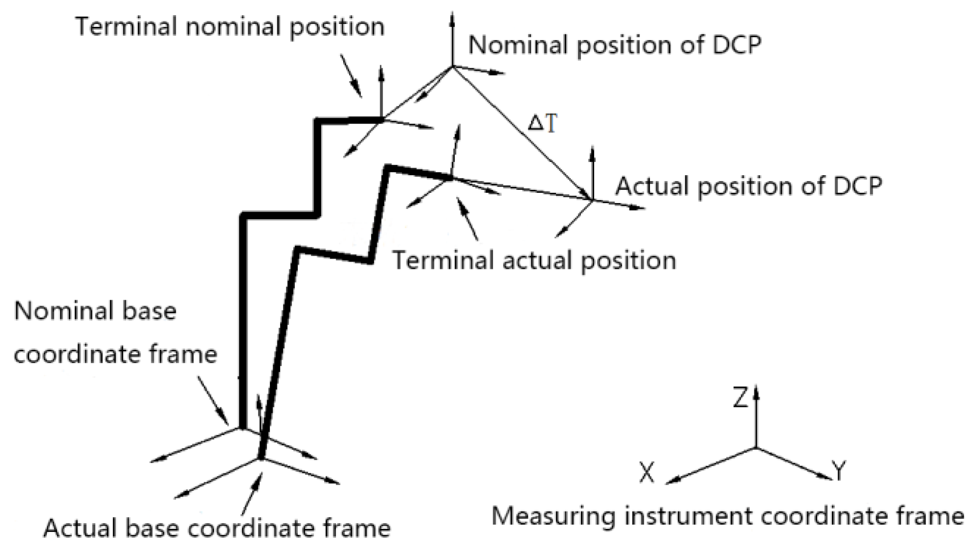
When calculating the RBCS, the position of the end of the robot is read directly from the robot instructor, which is different from the actual position. Therefore, the position of the RBCS obtained by calculation is also different from that of the MICS. Similarly, when measuring and calculating the position of DCP, there are some errors due to the influence of measurement disturbance. The DCP position and the RBCS position calculated by the model are defined as nominal DCP coordinate system and nominal based coordinate system, as shown in Figure 3. The actual position of DCP is measured directly by the measuring instrument. The factors affecting the nominal position and actual position of DCP include robot kinematics parameter error, RBCS position error and DCP coordinate system position error. The following three aspects will be analyzed separately.

3.1. Robot Kinematics Parameter Errors

Because of wear and deformation, the parameters of the robot’s links have errors, which lead to the deviation between the actual value and the nominal value of the robot’s kinematics model parameters. The parameter errors affecting the robot pose error are

$$\begin{gathered} \Delta \theta =\left[\Delta {\theta }_1,\Delta {\theta }_2,\Delta {\theta }_3,\Delta {\theta }_4,\Delta {\theta }_5,\Delta {\theta }_6\right]; \\ \Delta a=\left[\Delta a_1,\Delta a_2,\Delta a_3,\Delta a_4,\Delta a_5,\Delta a_6\right]; \\ \Delta \alpha =\left[\Delta {\alpha }_1,\Delta {\alpha }_2,\Delta {\alpha }_3,\Delta {\alpha }_4,\Delta {\alpha }_5,\Delta {\alpha }_6\right]; \\ \Delta d=\left[\Delta d_1,\Delta d_2,\Delta d_3,\Delta d_4,\Delta d_5,\Delta d_6\right]; \\ \Delta \beta =\left[\Delta {\beta }_1,\Delta {\beta }_2,\Delta {\beta }_3,\Delta {\beta }_4,\Delta {\beta }_5,\Delta {\beta }_6\right]. \end{gathered}$$

where $\Delta {\beta }_i$ only exists parallel axis, the non-parallel axis directly causes $\Delta {\beta }_i=0$.

The actual transformation relationship between the RBCS and FCS can be represented by a model with parameter errors:

$$\begin{gathered} {}_0{}^{6}T={}_0{}^{1}T·{}_1{}^{2}T·{}_2{}^{3}T·{}_3{}^{4}T·{}_4{}^{5}T·{}_5{}^{6}T \\ ={\prod }_{i=1}^{6}R\left(z_{i-1},{\theta }_i+\Delta {\theta }_i\right)·T\left(z_{i-1},d_i+\Delta d_i\right)·T\left(x_i,a_i+\Delta a_i\right)·R\left(x_i,{\alpha }_i+\Delta {\alpha }_i\right)· \\ R\left(y_i,{\beta }_i+\Delta {\beta }_i\right). \end{gathered}$$

(13)

In the equation, $R$ means rotation transformation, and $T$ means translation transformation.

3.2. Parameter Errors of Robot Base Coordinate System

The errors of the RBCS represents the parameter errors of the transformation model from the MICS to the RBCS. Let ${}_C{}^{0}T$ be the transformation model from the MICS to the RBCS. The nominal pose matrix of the RBCS calculated by Equation (13) in the MICS can be represented as follows:

$${}_C{}^{0}T^N=\left(\begin{array}{cccc}{n}_x& o_x& a_x& T_x\\ n_y& o_y& a_y& T_y\\ n_z{}_{}& o_z& a_z& T_z\\ 0& 0& 0& 1\end{array}\right).$$

(14)

In Equation (14), there are 12 parameters representing position and pose. To reduce the number of parameters to be identified, it can be rewritten as a 6-parameter model composed with a translation transformation and three rotational transformations.

$${}_C{}^{0}T^N=T(x_c,y_c,z_c)R(x_c,\theta x_c)R(y_c,\theta y_c)R(z_c,\theta z_c).$$

(15)

Therefore, the parameter errors of the RBCS are: $[\Delta x_c,\Delta y_c,\Delta z_c,\Delta \theta x_c,\Delta \theta y_c,\Delta \theta z_c]$.

The parameter errors are added to ${}_C{}^{0}T$ to get the actual pose model of the RBCS as

$$\begin{array}{c}{}_C{}^{0}T{}^R=T(x_c+\Delta x_c,y_c+\Delta y_c,z_c+\Delta z_c)R(x_c,\theta x_c+\Delta \theta x_c)\\ \begin{array}{ccc}& & \end{array}R(y_c,\theta y_c+\Delta \theta y_c)R(z_c,\theta z_c+\Delta \theta z_c).\end{array}$$

(16)

In the equation, the superscript R represents the actual value.

3.3. DCP Coordinate System Parameter Errors

The parameter errors of the DCP coordinate system represent the parameter errors of the transformation model from the FCS to the DCP coordinate system. Assuming that the pose transformation matrix of the robot’s DCP coordinate system is ${}_6{}^{D}T$ relative to that of the robot’s end FCS, the transformation model from the robot’s end flange to the DCP coordinate system can also be obtained by imitating the error derivation process of the RBCS:

$$\begin{array}{l}{}_6{}^{D}T^R=T\left(x_D+\Delta x_D,y_D+\Delta y_D,z_D+\Delta z_D\right)R\left(x_D,\theta x_D+\Delta \theta x_D\right)\\ R\left(y_D,\theta y_D+\Delta \theta y_D\right)R\left(z_D,\theta z_D+\Delta \theta z_D\right).\end{array}$$

(17)

After the above three pose models are obtained, they can be integrated into the actual DCP pose model in the MICS. Set T as the transformation matrix of the MICS to the robot DCP coordinate system:

$$T=\left(\begin{array}{cc}\mathit{R}& \mathit{P}\\ 0& 1\end{array}\right).$$

(18)

In the equation, $\mathit{R}$ denotes the pose of the DCP coordinate system in the MICS, $\mathit{P}$ denotes the position of the DCP coordinate system in the MICS.

The actual pose of DCP can be represented as

$$T^R={}_C{}^{0}T^R·{}_0{}^{6}T^R·{}_6{}^{D}T^R.$$

(19)

Parameter errors affecting DCP pose accuracy:

$$\begin{gathered} q=\left[\Delta x_C,\Delta y_C,\Delta z_C,\Delta \theta x_C,\Delta \theta y_C,\Delta \theta z_C,\Delta {\theta }_1~\Delta {\theta }_6,\Delta d_1~\Delta d_6, \\ \Delta a_1~\Delta a_6,\Delta {\alpha }_1~\Delta a_6,\Delta {\beta }_1~\Delta {\beta }_6,\Delta x_D,\Delta y_D,\Delta z_D,\Delta \theta x_D,\Delta \theta y_D, \\ \Delta \theta z_D\right]. \end{gathered}$$

Position error model is comparatively more general, so the pose error of DCP is neglected. Assuming the set of parameter errors is $\Delta \mathit{q}$, based on Equation (19), the actual position model of DCP can be expressed as follows:

$${\mathit{P}}^R=\left(\begin{array}{c}{P}_x{}^R\\ P_y{}^R\\ P_z{}^R\end{array}\right)=\left(\begin{array}{c}{f}_{{\mathit{P}}_x}(\mathit{q}+\Delta \mathit{q})\\ f_{{\mathit{P}}_y}(\mathit{q}+\Delta \mathit{q})\\ f_{{\mathit{P}}_z}(\mathit{q}+\Delta \mathit{q})\end{array}\right).$$

(20)

Therefore, the mathematical relationship between the DCP position error and the parameters errors of the model can be represented as

$$\Delta {\mathit{P}}^R=\left(\begin{array}{c}\Delta P_x{}^R\\ \Delta P_y{}^R\\ \Delta P_z{}^R\end{array}\right)=\left(\begin{array}{c}{f}_{{\mathit{P}}_x}(\mathit{q}+\Delta \mathit{q})-f_{{\mathit{P}}_x}(\mathit{q})\\ f_{{\mathit{P}}_y}(\mathit{q}+\Delta \mathit{q})-f_{{\mathit{P}}_y}(\mathit{q})\\ f_{{\mathit{P}}_z}(\mathit{q}+\Delta \mathit{q})-f_{{\mathit{P}}_z}(\mathit{q})\end{array}\right).$$

(21)

In Equation (21), the relationship between the DCP position error and the parameter error is nonlinear, so it is difficult to solve them directly. Therefore, it can be analyzed from the perspectives of partial differential. For the model with n parameter errors, Equation (21) can be rewritten as follows:

$$\Delta {\mathit{P}}^R=\left(\begin{array}{c}\Delta P_x{}^R\\ \Delta P_y{}^R\\ \Delta P_z{}^R\end{array}\right)=\left(\begin{array}{cccc}\frac{\partial f_{{\mathit{P}}_x}}{\partial \Delta q_1}& \frac{\partial f_{{\mathit{P}}_x}}{\partial \Delta q_2}& \dots & \frac{\partial f_{{\mathit{P}}_x}}{\partial \Delta q_n}\\ \frac{\partial f_{{\mathit{P}}_y}}{\partial \Delta q_1}& \frac{\partial f_{{\mathit{P}}_y}}{\partial \Delta q_2}& \dots & \frac{\partial f_{{\mathit{P}}_x}}{\partial \Delta q_n}\\ \frac{\partial f_{{\mathit{P}}_z}}{\partial \Delta q_1}& \frac{\partial f_{{\mathit{P}}_z}}{\partial \Delta q_2}& \dots & \frac{\partial f_{{\mathit{P}}_x}}{\partial \Delta q_n}\end{array}\right)\left(\begin{array}{c}\Delta q_1\\ \Delta q_2\\ ⋮\\ \Delta q_n\end{array}\right).$$

(22)

The Equation (22) can be simplified to

$$\mathit{\epsilon }=M\Delta \mathit{q}.$$

In the equation, $\mathit{\epsilon }$ denotes the DCP position error, $\Delta \mathit{q}$ denotes all the parameter errors of the calibration model, and $M$ denotes the error coefficient matrix.

4. Parameter Error Identification and Compensation

4.1. Redundancy Parameter Analysis

In Section 2.3, the robot DCP position error model is obtained: $\mathit{\epsilon }=M\Delta \mathit{q}$. In the equation, $\mathit{\epsilon }$ can be measured by measuring equipment; $M$ represents the error coefficient matrix, which can be derived by error model; $\Delta \mathit{q}$ is the parameter error need to be solved. Therefore, in order to get the solution of parameter error, it only needs to take the measured pose error $\mathit{\epsilon }$ into the error model and solve $\Delta \mathit{q}$. However, there may be redundancy between the kinematics parameters of the robot, which may lead to the correlation among the columns of the coefficient matrix $M$. And it will directly affect the accuracy of $\Delta \mathit{q}$.

Let ${}_i{}^{i+1}T$ denote the homogeneous transformation from {i} to {i+1} of the LCS (link coordinate system) of robot. When only the pose transformation is considered, $\beta \approx 0$ can be directly brought into Equation (1). The result is as follows:

$${}_i{}^{i+1}T=\left(\begin{array}{cccc}c{\theta }_i& -s{\theta }_{i}c{\alpha }_i& s{\theta }_{i}s{\alpha }_i& a_{i}c{\theta }_i\\ s{\theta }_i& c{\theta }_{i}c{\alpha }_i& -c{\theta }_{i}s{\alpha }_i& a_{i}s{\theta }_i\\ 0& s{\alpha }_i& c{\alpha }_i& d_i\\ 0& 0& 0& 1\end{array}\right).$$

(23)

According to the differential kinematics of the robot, the differential transformation relation between the LCS {i} and {i+1} can be obtained by combining Equation (23):

$$\left(\begin{array}{c}d{x}_{i+1}\\ d{y}_{i+1}\\ d{z}_{i+1}\\ \delta x_{i+1}\\ \delta y_{i+1}\\ \delta z_{i+1}\end{array}\right)=\left(\begin{array}{cccccc}\mathrm{c}{\theta }_i& s{\theta }_i& 0& -d_{i}s{\theta }_i& d_{i}c{\theta }_i& 0\\ -c{\alpha }_{i}s{\theta }_i& c{\alpha }_{i}c{\theta }_i& s{\alpha }_i& a_{i}s{\alpha }_{i}s{\theta }_i-d_{i}c{\alpha }_{i}c{\theta }_i& -a_{i}s{\alpha }_{i}c{\theta }_i-d_{i}c{\alpha }_{i}s{\theta }_i& a_{i}c{\alpha }_i\\ s{\alpha }_{i}s{\theta }_i& -s{\alpha }_{i}c{\theta }_i& c{\alpha }_i& a_{i}c{\alpha }_{i}s{\theta }_i+d_{i}s{\alpha }_{i}c{\theta }_i& -a_{i}c{\alpha }_{i}c{\theta }_i+d_{i}s{\alpha }_{i}s{\theta }_i& -a_{i}s{\alpha }_i\\ 0& 0& 0& c{\theta }_i& s{\theta }_i& 0\\ 0& 0& 0& -c{\alpha }_{i}s{\theta }_i& c{\alpha }_{i}c{\theta }_i& s{\alpha }_i\\ 0& 0& 0& s{\alpha }_{i}s{\theta }_i& s{\alpha }_{i}c{\theta }_i& c{\alpha }_i\end{array}\right)\left(\begin{array}{c}d{x}_i\\ d{y}_i\\ d{z}_i\\ \delta x_i\\ \delta y_i\\ \delta z_i\end{array}\right)={}_i{}^{i+1}J{}_{}\mathrm{D}.$$

(24)

In the equation, ${}_i{}^{i+1}J$ is an error coefficient matrix, representing the transformation matrix from the LCS {i} to {i+1} with differential motion.

In ${}_i{}^{i+1}J$, for a general robot with rotating joints, ${\theta }_i$ are variables and ${\alpha }_i$ are constants. Therefore, only the third and sixth columns of ${}_i{}^{i+1}J$ remain unchanged, and the rest of the columns change with ${\theta }_i$. Let ${}_{i+1}{}^{i+1}J$ represent the differential transformation matrix of the coordinate system {i} relative to itself:

$${}_{i+1}{}^{i+1}J=\left(\begin{array}{cccccc}1& 0& 0& 0& 0& 0\\ 0& 1& 0& 0& 0& 0\\ 0& 0& 1& 0& 0& 0\\ 0& 0& 0& 1& 0& 0\\ 0& 0& 0& 0& 1& 0\\ 0& 0& 0& 0& 0& 1\end{array}\right).$$

(25)

From the relationship between column vectors in ${}_i{}^{i+1}J$ and ${}_{i+1}{}^{i+1}J$, the relation can be found that:

$$\{\begin{array}{l}{}_i{}^{i+1}J_3=s{\alpha }_i{}_{i+1}{}^{i+1}J_2+s{\alpha }_i{}_{i+1}{}^{i+1}J_3\\ {}_i{}^{i+1}J_6=a_{i}c{\alpha }_i{}_{i+1}{}^{i+1}J_2-a_{i}s{\alpha }_i{}_{i+1}{}^{i+1}J_3+s{\alpha }_i{}_{i+1}{}^{i+1}J_4+c{\alpha }_i{}_{i+1}{}^{i+1}J_5\end{array}.$$

(26)

In the Equation (26), ${}_i{}^{i+1}J_k$ and ${}_{i+1}{}^{i+1}J_k$ denote the kth column of matrix ${}_i{}^{i+1}J_k$ and ${}_{i+1}{}^{i+1}J_k$ respectively.

Assuming that the degree of freedom of the robot is N, both sides of above equation are multiplied by ${}_{i+1}{}^{N}J$, so that the differential errors of the two coordinate systems are converted to the end of the robot:

$$\{\begin{array}{l}{}_i{}^{N}J_3=s{\alpha }_i{}_{i+1}{}^{N}J_2+s{\alpha }_i{}_{i+1}{}^{N}J_3\\ {}_i{}^{N}J_6=a_{i}c{\alpha }_i{}_{i+1}{}^{N}J_2-a_{i}s{\alpha }_i{}_{i+1}{}^{N}J_3+s{\alpha }_i{}_{i+1}{}^{N}J_4+c{\alpha }_i{}_{i+1}{}^{N}J_5\end{array}.$$

(27)

Equation (27) shows that the influence of the differential errors $d{z}_i$ and $\delta z_i$ of the LCS {i} on its end can be expressed by the differential errors of the LCS {i + 1}; that is, the differential errors $d{z}_i$ and $\delta z_i$ of the LCS {i} are related to the differential errors of the LCS {i + 1}, and are redundant. It shows that $d{z}_i$ and $\delta z_i$ are redundant parameters in the transformation model of the MICS to the RBCS. The differential error of each LCS of robot model needs to be transformed into kinematic model parameter error:

$$\left(\begin{array}{c}d{x}_i\\ d{y}_i\\ d{z}_i\\ \delta x_i\\ \delta y_i\\ \delta z_i\end{array}\right)=\left(\begin{array}{ccccc}0& 0& 1& 0& 0\\ a_{i}c{\alpha }_i& s{\alpha }_i& 0& 0& 0\\ -a_{i}s{\alpha }_i& c{\alpha }_i& 0& 0& 0\\ 0& 0& 0& 1& 0\\ s{\alpha }_i& 0& 0& 0& 1\\ c{\alpha }_i& 0& 0& 0& 0\end{array}\right)\left(\begin{array}{c}\Delta {\theta }_i\\ \Delta d_i\\ \Delta a_i\\ \Delta {\alpha }_i\\ \Delta {\beta }_i\end{array}\right)=G_i\Delta q_i.$$

(28)

Equation (28) shows that the variables in $G_i$ are only $a$ and $\alpha$. Different values of $a$ and $\alpha$ are analyzed and the results are shown in

Table 1. Redundancy identification of robot kinematics parameters.

Identification Condition	Redundancy Parameter
${\alpha }_i\ne 0$	None
${\alpha }_i=0\&a_i\ne 0$	$\Delta d_i$
${\alpha }_i=0\&a_i=0$	$\Delta d_i$, $\Delta {\theta }_i$

.

4.2. Parameter Identification Algorithm

The differential error model of position and posture of robot DCP is determined as follows:

$$\mathit{\epsilon }=M\Delta \mathit{q}.$$

(29)

Assuming that $\Delta \mathit{q}$ removes redundant parameters, the number of identifiable parameters is N, then $M_p$ and $M_{\delta }$ are both the coefficient matrices of 3 × N. To solve N parameter errors, at least N equations are needed, that is, the position of N/3 sampling points must be measured before the solution to the equations can be obtained. In actual measurement, there may be unavoidable error factors that interfere with the accuracy of the solution. Therefore, a large amount of data needs to be used to fit the model. Assuming that the group K (K > N/3) position data of robot can be measured, the equations can be obtained:

$$\{\begin{array}{c}{M}_{11}\Delta q_1+M_{12}\Delta q_2+\cdots +M_{1N}\Delta q_N=\Delta {\mathrm{P}}_{1x}\\ M_{21}\Delta q_1+M_{22}\Delta q_2+\cdots +M_{2N}\Delta q_N=\Delta {\mathrm{P}}_{1y}\\ M_{31}\Delta q_1+M_{32}\Delta q_2+\cdots +M_{3N}\Delta q_N=\Delta {\mathrm{P}}_{1z}\\ ⋮\\ M_{11}\Delta q_1+M_{12}\Delta q_2+\cdots +M_{1N}\Delta q_N=\Delta {\mathrm{P}}_{Kx}\\ M_{21}\Delta q_1+M_{22}\Delta q_2+\cdots +M_{2N}\Delta q_N=\Delta {\mathrm{P}}_{Ky}\\ M_{31}\Delta q_1+M_{32}\Delta q_2+\cdots +M_{3N}\Delta q_N=\Delta {\mathrm{P}}_{Kz}\end{array}.$$

(30)

Equation (30) is an overdetermined equation set, which can be solved by least square method:

$$\Delta \mathit{q}=M^{+}\mathit{\epsilon }.$$

(31)

The $M^{+}$ in the equation represents the generalized inverse of the coefficient matrix $M$.

4.3. Parameter Error Compensation Algorithm

After the error of each parameter is obtained by the identification algorithm, the revised parameters can be input into robot controller to achieve the robot calibration. However, for most robot controllers, the manufacturer will not authorize the user to modify the robot structure parameters directly. In this case, only the joint angle $\theta$ can be adjusted, while other kinematics parameters cannot be modified directly.

The errors of $d$, $a$, $\alpha$, $\beta$ in kinematics parameters have different effects on pose errors under different robot pose. In this paper, Newton Iteration Method is used to adjust the joint angle $\theta$ to compensate the pose deviation caused by the errors of $d$, $a$, $\alpha$, $\beta$ in kinematics parameters, so as to achieve the compensation of pose accuracy of the robot end. Assuming that the robot’s target pose is $T^N$, $\Delta d_i{,}^{}\Delta a_i{,}^{}\Delta {\alpha }_i{,}^{}\Delta {\beta }_i$ are substituted into the model to obtain $T^R$, and then the difference between the nominal pose and the actual ones is used to calculate the partial derivative of each joint angle:

$$T^N-T^R=\frac{\partial T}{\partial {\theta }_i}\Delta {\theta }^R{}_i+\frac{\partial T}{\partial {\theta }_2}\Delta {\theta }^R{}_2+\frac{\partial T}{\partial {\theta }_3}\Delta {\theta }^R{}_3+\frac{\partial T}{\partial {\theta }_4}\Delta {\theta }^R{}_4+\frac{\partial T}{\partial {\theta }_5}\Delta {\theta }^R{}_5+\frac{\partial T}{\partial {\theta }_6}\Delta {\theta }^R{}_6.$$

(32)

5. Robot Calibration Experiment

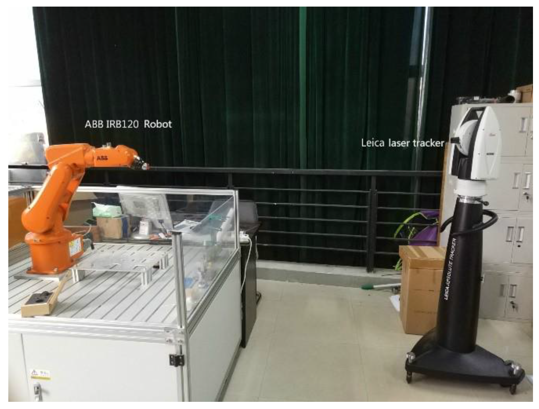
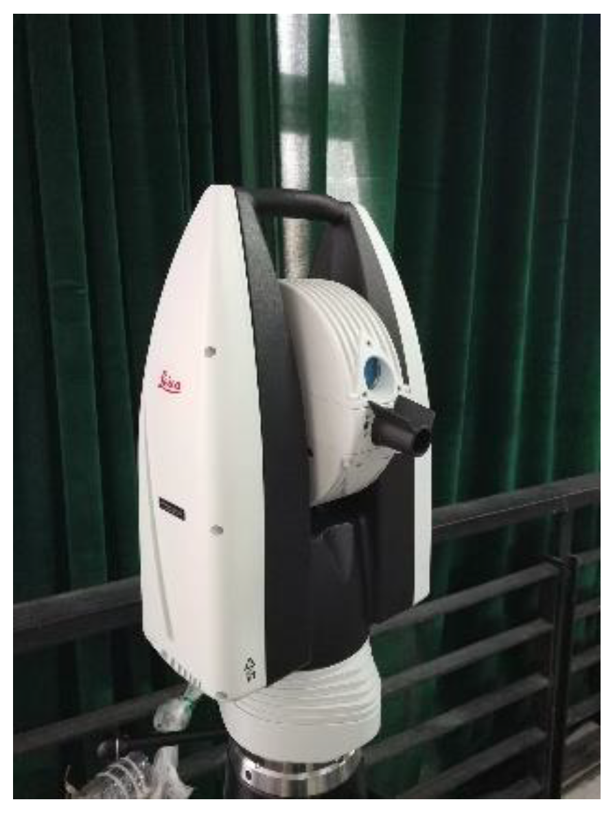
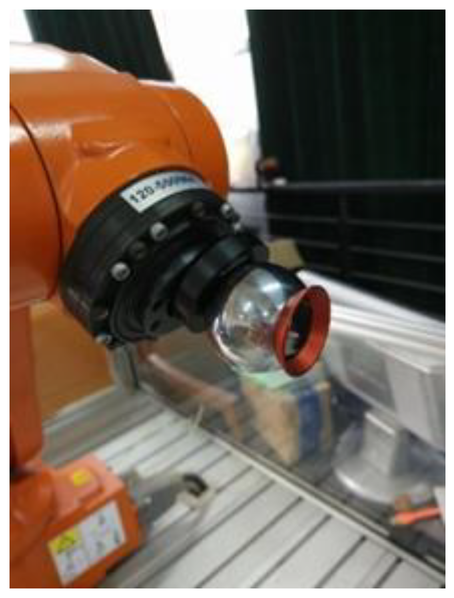
The experimental object of this paper is IRB120 industrial robot. The measurement system is shown in Figure 4. The measuring instrument is Leica AT960MR absolute laser tracker as shown in Figure 5, which can measure the end position of the robot with laser receiving target ball as shown in Figure 6. The software SpatialAnalyzer (SA) can be used for data acquisition connecting Leica AT960MR, data processing, and exporting the data of the robot end position based on its own coordinate system. Using the coordinate conversion method mentioned in Section 2.3, the data in AT960MR coordinate system and the data in the RBCS are fitted with the least square method. The transformational matrix between the coordinate system of AT960MR and the robot base can be obtained by Matlab software. So the data in laser tracker coordinate system can be converted to the RBCS. The measured robot end pose in AT960MR and the robot end pose displayed in the robot controller are unified into the same coordinate system for comparison.

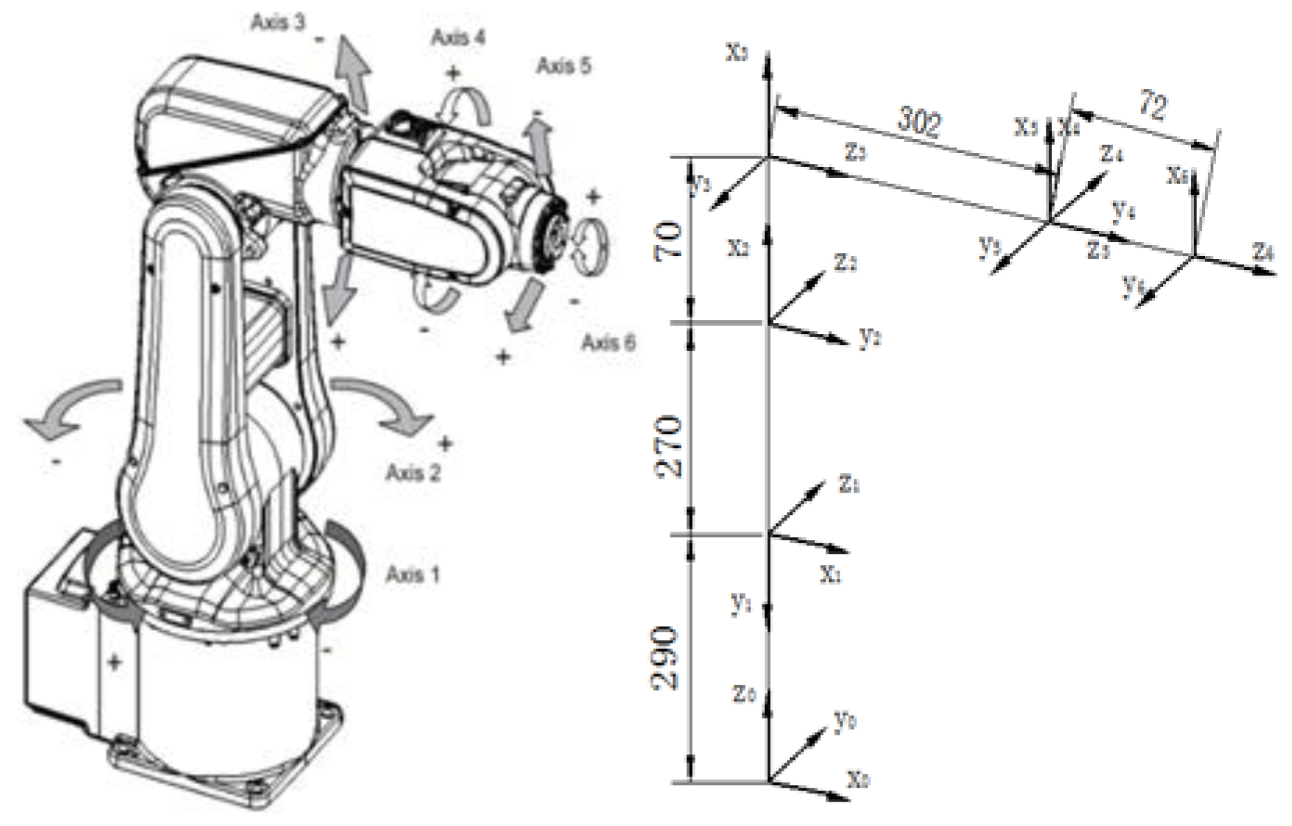
The first step of calibration experiment is modeling. First, the kinematics model of the robot is determined. The MDH model of the ABB IRB120 robot is expressed in Figure 7, and the MDH parameters are expressed in

Table 2. Nominal parameters of robot MDH model.

Axis i	${\mathit{\theta }}_{\mathit{i}}$	${\mathit{d}}_{\mathit{i}}$	${\mathit{a}}_{\mathit{i}}$	${\mathit{\alpha }}_{\mathit{i}}$	${\mathit{\beta }}_{\mathit{i}}$
1	${\theta }_1$	290	0	−90	−
2	${\theta }_2-90$	0	270	0	0
3	${\theta }_3$	0	70	−90	−
4	${\theta }_4$	302	0	90	−
5	${\theta }_5$	0	0	−90	−
6	${\theta }_6$	72	0	0	−

.

The nominal transformation model parameters can be obtained by calibrating the robot DCP coordinate system and the RBCS as shown in

Table 3. Nominal parameters of robot base coordinate transformation model.

$\mathit{x} \mathbf{(}\mathbf{mm}\mathbf{)}$	$\mathit{y} \mathbf{(}\mathbf{mm}\mathbf{)}$	$\mathit{z} \mathbf{(}\mathbf{mm}\mathbf{)}$	$\mathit{R}\mathit{x} (°)$	$\mathit{R}\mathit{y} (°)$	$\mathit{R}\mathit{z} (°)$
−1384.05	1448.6	−391.47	1.6	1.8	60.1

and

Table 4. Nominal parameters of robot DCP coordinate transformation model.

$\mathit{x} \mathbf{(}\mathbf{mm}\mathbf{)}$	$\mathit{y} \mathbf{(}\mathbf{mm}\mathbf{)}$	$\mathit{z} \mathbf{(}\mathbf{mm}\mathbf{)}$	$\mathit{R}\mathit{x} (°)$	$\mathit{R}\mathit{y} (°)$	$\mathit{R}\mathit{z} (°)$
−27.31	−19.82	25.71	−	−	−

:

According to the analysis of redundancy parameters in Section 3.1, the error of redundancy parameters in the kinematics model of robot is $\Delta d_2$, $\Delta d_6$ and $\Delta {\theta }_6$, and the redundancy parameters in the transformation model of RBCS are $\Delta z$ and $\delta z$. So there are 28 discernible parameters in this calibration experiment. Fifty groups of robot pose data are taken as calibration points in robot workspace, and the error of robot parameters is computed.

The parameters errors of the identified error models are expressed in

Table 5. Parameters error of robot base coordinate system (RBCS) error model.

$\mathbf{\Delta }\mathit{x} (\mathbf{mm})$	$\mathbf{\Delta }\mathit{y} (\mathbf{mm})$	$\mathbf{\Delta }\mathit{z} (\mathbf{mm})$	$\mathbf{\Delta }\mathit{R}\mathit{x} (°)$	$\mathbf{\Delta }\mathit{R}\mathit{y} (°)$	$\mathbf{\Delta }\mathit{R}\mathit{z} (°)$
0.2451	−0.1712	−	0.0348	0.0478	−

,

Table 6. Parameters error of DCP coordinate system error model of robot.

$\mathbf{\Delta }\mathit{x} (\mathbf{mm})$	$\mathbf{\Delta }\mathit{y} (\mathbf{mm})$	$\mathbf{\Delta }\mathit{z} (\mathbf{mm})$	$\mathbf{\Delta }\mathit{R}\mathit{x} (°)$	$\mathbf{\Delta }\mathit{R}\mathit{y} (°)$	$\mathbf{\Delta }\mathit{R}\mathit{z} (°)$
0.0746	0.0849	−0.0687	−	−	−

and

Table 7. Parameters error based on end pose recognition.

Axis i	$\mathbf{\Delta }\mathit{\theta } (°)$	$\mathbf{\Delta }\mathit{d} (\mathbf{mm})$	$\mathbf{\Delta }\mathit{a} (\mathbf{mm})$	$\mathbf{\Delta }\mathit{a} (°)$	$\mathbf{\Delta }\mathit{\beta } (°)$
1	−0.0616	−0.1641	0.0745	−0.0883	−
2	−0.0398	−	−0.2474	0.0695	0.0701
3	0.0801	0.1487	0.2094	−0.0962	−
4	0.0997	0.1345	−0.1471	−0.1321	−
5	0.0157	0.0745	−0.0677	0.1027	−
6	−	−	0.0224	−0.0754	−

.

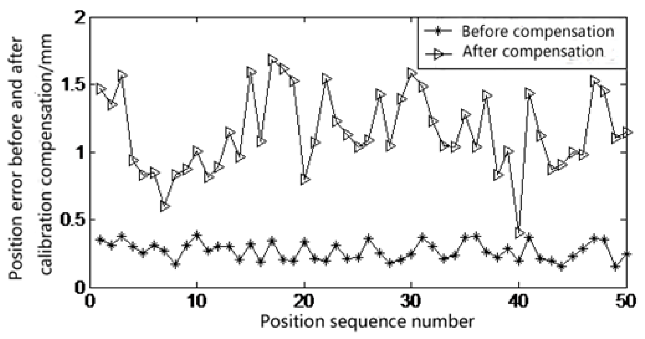
The calibrated parameter error is substituted into the model by the compensation method proposed in Section 3.3. After measurement, the robot pose error before and after compensation is obtained as shown in Figure 8. The results of compensation analysis are expressed in

Table 8. Position error before and after calibration point compensation.

	Before Calibration	After Calibration	Decrease
Mean position error (mm)	1.2248	0.2678	78.1%
Maximum position error (mm)	1.6780	0.3876	76.9%
Standard deviation	1.4688	0.3525	76.0%

.

Comparing Table 7 and Table 8, the compensation effect of 50 groups of calibration points is better than that of 100 groups of sampling points. This is because the position error of the robot end is not only related to the parameter error of the robot kinematics model, but also influenced by many other factors. In addition, the error caused by measurement disturbance is unavoidable in the process of measurement. Therefore, in the process of identifying parameter errors, a group of optimal solutions are obtained according to the position error characteristics of all 50 groups of calibration points. In the 100 groups of sampling points except the calibration points, some of them differ greatly from the position error characteristics of the calibration points, and the calibration results have comparatively poor compensation effect on these sampling points. Therefore, the overall calibration effect is not as good as the compensation for the calibration point.

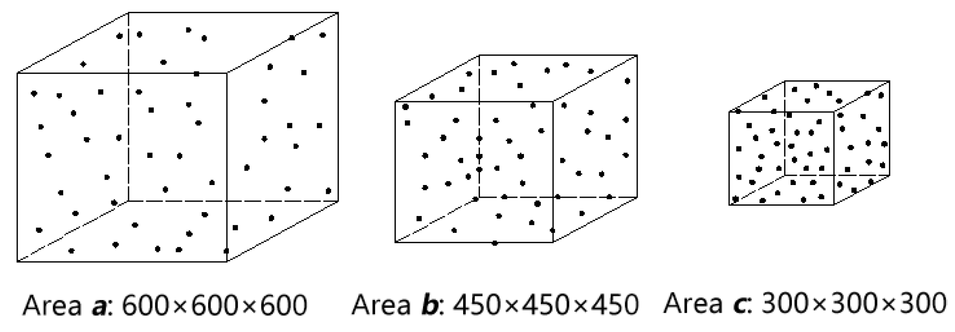
In order to verify the correlation between calibration effect and the distribution of calibration points, add the following experiments: Take the point [300, 300, 300] in the RBCS as the center, respectively establish three kinds of cube space with the size of 600 mm, 450 mm, and 300 mm, defined as areas a, b, and c respectively. Fifty groups data of robot’s pose are measured in the three areas, respectively, and ensure that the pose of sampling points are evenly distributed in each space, as shown in Figure 9.

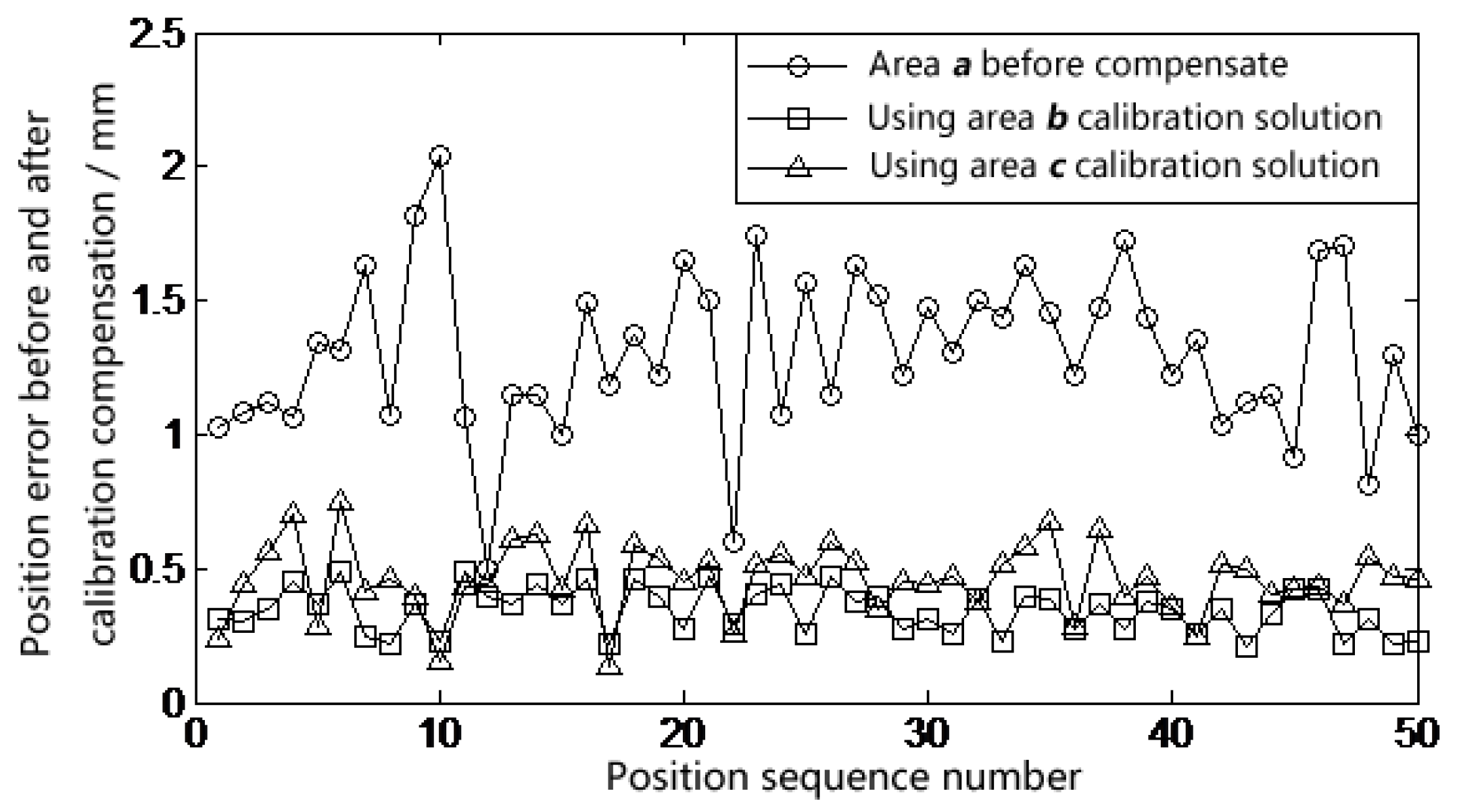
The sampling points in the b and c areas are taken as calibration points to the position error identification algorithm. The calculated parameters errors results are compensated respectively to the sampling points in area a. Calculating and comparing the errors before and after calibration, the experimental results are shown in Figure 10 and

Table 9. Compensation effect of sampling points in area a.

	Area c Position Error Average (mm)
	Before Calibration	After Calibration	Decrease
Area b calibration solution to compensate area a sampling points	1.3052	0.3432	73.7%
Area c calibration solution to compensate area a sampling points		0.4623	64.5%

.

From the above results, it can be seen that the more uniform the selected calibration points are distributed in a certain space, the better effect of the calibration solution is.

In comparison, these literature [14,15,16] all use the laser tracker as the measuring instrument to improve the absolute positioning accuracy of the robot. Literature [14] improved the accuracy by about one time. Literature [15] uses different calibration methods to reduce the maximum error by about 60%, but the experiment only measured the data of 20 points, and the optimized maximum positioning deviation is still 1.30 mm. Literature [16] measures 1000 points in a certain working space, which can reduce the mean value of absolute positioning accuracy from 0.981 to 0.292, and the error is reduced by about 70%. The results of this experiment are obviously better than the first two paper. Compared with the method in literature [16], we take relatively lesser number of points, but it can achieve nearly the same accuracy improvement effect.

6. Summary

In order to allow robots to be applied in high-precision fields, this paper studies the methods of improving the accuracy of robots. Firstly, the DCP coordinate system is established from the point of perspectives of actual measurement, and the comparative general measurement methods of DCP coordinate system and RBCS are given, so that the complete error model is established. Then use differential kinematics to establish a differential error model, and the error identification equation is obtained. The error of redundant parameters in the error model is analyzed, and the method of identifying the error of redundant parameters is given. Finally, a compensation method without modifying the parameters of the underlying model of the robot is proposed. Experiments show that the calibration method proposed in this paper can effectively reduce the end position error of the robot and has a certain research significance for robot precision improvement technology.

References

- Summers, M. Robot capability test and development of industrial robot positioning system for the aerospace industry. SAE Trans. 2005, 114, 1108–1118. [Google Scholar]
- Guerra, R.H.; Quiza, R.; Villalonga, A.; Arenas, J.; Castaño, F. Digital Twin-Based Optimization for Ultraprecision Motion Systems with Backlash and Friction. IEEE Access 2019, 7, 93462–93472. [Google Scholar] [CrossRef]
- Kelly, R.; Haber, R.; Haber-Guerra, R.E.; Reyes, F. Lyapunov Stable Control of Robot Manipulators: A Fuzzy Self-Tuning Procedure. Intell. Autom. Soft Comput. 1999, 5, 313–326. [Google Scholar] [CrossRef]
- Han, X.; Du, D.; Chen, Q.; Wang, G.; He, Y.; Sui, B. Research on Trajectory Accuracy Measurement of industrial robot based on kinematic analysis. Robot 2002, 24, 1–5. [Google Scholar]
- Hayati, S.; Mirmirani, M. Improving the absolute positioning accuracy of robot manipulators. J. Field Robot. 2010, 2, 397–413. [Google Scholar] [CrossRef]
- Judd, R.P.; Knasinski, A.B. A technique to calibrate industrial robots with experimental verification. IEEE Trans. Robot Autom. 1987, 6, 20–30. [Google Scholar] [CrossRef]
- Whitney, D.; Lozinski, C.; Rourke, J. Industrial Robot Forward Calibration Method and Results. J. Dyn. Syst. Meas. Control ASME 1986, 108, 1–8. [Google Scholar] [CrossRef]
- He, R.; Zhao, Y.; Yang, S.; Yang, S. Kinematic-Parameter Identification for Serial-Robot Calibration Based on POE Formula. Robot IEEE Trans. 2010, 26, 411–423. [Google Scholar]
- Wang, Y.; Wang, G.; Yun, C. A calibration method of kinematic parameters for serial industrial robots. Ind. Robot Int. J. 2014, 41, 157–165. [Google Scholar] [CrossRef]
- Xin, G.; Bo, F. Calibration procedure for a system of two coordinated manipulators. Int. J. Robot Autom. 1995, 10, 152–158. [Google Scholar]
- Wang, Z.; Xu, H.; Chen, G.; Sun, R.; Lining, S. A distance error based industrial robot kinematic calibration method. Ind. Robot Int. J. 2014, 41, 439–446. [Google Scholar] [CrossRef]
- Young, K.-Y.; Chen, J.-J.; Wang, C.-C. An automated robot calibration system based on a variable D-H parameter model. In Proceedings of the 35th IEEE Conference on Decision and Control, Kobe, Japan, 13 December 1996; Volume 1, pp. 881–886. [Google Scholar]
- Chen, J.; Chao, L.M. Positioning error analysis for robot manipulators with all rotary joints. Robot. Autom. IEEE J. 1987, 3, 539–545. [Google Scholar] [CrossRef]
- Ren, Y. Method of robot calibration based on laser tracker. Chin. J. Mech. Eng. 2007, 43, 195–200. [Google Scholar] [CrossRef]
- Wang, W.; Liu, L.; Wang, G.; Yun, C. Calibration method of robot base frame by quaternion form. J. Beijing Univ. Aeronaut Astronaut 2015, 41, 47–54. [Google Scholar]
- Nubiola, A.; Bonev, I.A. Absolute calibration of an ABB IRB 1600 robot using a laser tracker. Robot Comput. Integr. Manuf. 2013, 29, 236–245. [Google Scholar] [CrossRef]
- Bennett, D.J.; Hollerbach, J.M. Self-calibration of single-loop, closed kinematic chains formed by dual or redundant manipulators. In Proceedings of the 27th IEEE Conference on Decision and Control, Austin, TX, USA, 7–9 December 1988; Volume 1, pp. 627–629. [Google Scholar]
- Joubair, A.; Bonev, I.A. Non-kinematic calibration of a six-axis serial robot using planar constraints. Precis. Eng. 2015, 40, 325–333. [Google Scholar] [CrossRef]
- Legnani, G.; Tiboni, M. Optimal design and application of a low-cost wire-sensor system for the kinematic calibration of industrial manipulators. Mech. Mach. Theory 2014, 73, 25–48. [Google Scholar] [CrossRef]
- Denavit, J.; Hartenberg, R.S. A Kinematic Notation for Lower-Pair Mechanisms. ASME J. Appl. Mech. 1955, 22, 215–221. [Google Scholar]
- Hayati, S.A. Robot arm geometric link parameter estimation. In Proceedings of the 22nd IEEE Conference on Decision and Control, San Antonio, TX, USA, 14–16 December 1983; pp. 1477–1483. [Google Scholar]
- Park, I.-W.; Lee, B.-J.; Cho, S.-H.; Hong, Y.-D.; Kim, J.-H. Laser-Based Kinematic Calibration of Robot Manipulator Using Differential Kinematics. Mechatron. IEEE ASME Trans. 2012, 17, 1059–1067. [Google Scholar] [CrossRef]
Figure 1.
Detection Center Point (DCP) coordinate system position model.
Figure 2.
Actual measuring point and flange coordinate system (FCS).
Figure 3.
Actual position and nominal position of DCP.
Figure 4.
Experimental scenario.
Figure 5.
Leica laser tracker.
Figure 6.
Target ball.
Figure 7.
ABB IRB 120 MDH model.
Figure 8.
Position error curve of robot before and after compensation.
Figure 9.
Three kinds of space size and sampling point distribution.
Figure 10.
Compensation effect of sampling points in area a.