Analysis of the Propagation in High-Speed Interconnects for MIMICs by Means of the Method of Analytical Preconditioning: A New Highly Efficient Evaluation of the Coefficient Matrix

Abstract

The method of analytical preconditioning combines the discretization and the analytical regularization of a singular integral equation in a single step. In a recent paper by the author, such a method has been applied to a spectral domain integral equation formulation devised to analyze the propagation in polygonal cross-section microstrip lines, which are widely used as high-speed interconnects in monolithic microwave and millimeter waves integrated circuits. By choosing analytically Fourier transformable expansion functions reconstructing the behavior of the fields on the wedges, fast convergence is achieved, and the convolution integrals are expressed in closed form. However, the coefficient matrix elements are one-dimensional improper integrals of oscillating and, in the worst cases, slowly decaying functions. In this paper, a novel technique for the efficient evaluation of such kind of integrals is proposed. By means of a procedure based on Cauchy integral theorem, the general coefficient matrix element is written as a linear combination of fast converging integrals. As shown in the numerical results section, the proposed technique always outperforms the analytical asymptotic acceleration technique, especially when highly accurate solutions are required.

1. Introduction

The latest advances in the development of integrated circuit technology have increased the attractivity of microstrip transmission lines for the realization of high-speed interconnects in monolithic microwave and millimeter waves integrated circuits (MIMICs). In this contest, the width and the thickness of the metallic region can be comparable, and the transverse cross-section is closed to a trapezoidal shape due to the etching undercuts, or because of the electrolytical growth process. For all these reasons, the classical approaches, based on the modeling of the metallic region as a zero-thickness flat strip, are inappropriate for an accurate analysis of the propagation. Great attention has been paid in the last few decades to developing techniques which are able to evaluate the effect of the thickness and the cross-sectional shape of the metallic strip on the propagation [1,2,3,4,5,6,7,8,9,10]. Among others, integral equation formulations have been widely preferred.

In order to search for the solution of an integral equation which cannot be expressed in a closed form, a discretization scheme has to be provided. On the other hand, it is well-known that a direct discretization can lead to ill-conditioned and/or dense matrices for which the convergence of the approximate solution to the exact one, if it exists, cannot be guaranteed. A possible way to overcome this problem is the use of compression techniques [11,12], the Nyström method [13,14], or the direct formulation of the problem in terms of a Fredholm second-kind integral equation [15], just to give some examples.

In a recent paper [16], the analysis of bound and leaky modes propagation in single and coupled polygonal cross-section microstrip lines was carried out by generalizing the techniques presented in Refs. [17,18,19,20,21,22,23,24,25,26,27,28,29,30] for the analysis of propagation, radiation and scattering problems. The problem has been formulated as a homogeneous one-dimensional electric field integral equation (EFIE) in the spectral domain. A converging matrix equation has been achieved by means of the method of analytical preconditioning (MAP) [31], i.e., the Galerkin method, with suitable expansion functions such that Steinberg’s theorems can be applied [32]. In Ref. [16], this goal was reached by selecting expansion functions with a closed form Fourier transform reconstructing the physical behavior of the unknowns, even on the wedges. As a result, just a few expansion functions are enough to reconstruct the solution with good accuracy. Moreover, the Galerkin projection integrals have been written in closed form, thus leading to coefficient matrix elements expressed as combinations of one-dimensional integrals over the selected inverse Fourier transform integration path.

Unfortunately, the numerical evaluation of the coefficient matrix elements is burdensome. Since the expansion functions are continuous functions defined on finite supports, their spectral domain counterparts are oscillating functions with an algebraic asymptotic decay along the inverse Fourier transform integration path. For this reason, the coefficient matrix elements are improper integrals whose integrands are oscillating functions, which can have a slow asymptotic decay. As such, the simulations can be time-consuming when highly accurate solutions are searched for. A classical way to overcome this problem is the extraction of suitable asymptotic contributions from the integrands, such that the integrals of the extracted contributions can be expressed in closed form [33,34,35]. Unfortunately, such a technique leads to accelerated integrands with a faster but still algebraic decay, and it does not modify the asymptotic oscillating behavior of the integrands themselves. As a result, a slower and slower numerical convergence is expected as the accuracy required for the solution increases.

Recently, a different perspective was proposed in Refs. [36,37,38,39,40,41,42,43]. Instead of trying to speed up the convergence of the slowly converging integrals detailed above, fast-converging alternative expressions have been individuated. This can be done by means of a suitable application of the Cauchy integral theorem, which takes advantage of the mathematical properties of the integrands. Even if a general and common line of reasoning can be individuated for all the procedures presented in these papers, each of them is devised for the solution of a specific problem.

Following the same line of reasoning, in this paper, a new fast-converging expression for the improper integrals of oscillating and slowly decaying functions, arising from the analysis of the propagation in polygonal cross-section microstrip lines when an EFIE formulation in the spectral domain is discretized by means of MAP, is provided. A brief overview of the formulation of the problem and the discretization technique adopted in Ref. [16] is presented in Section 2. Section 3 is devoted to the fast evaluation of the coefficient matrix elements: the general improper integral, whose integrand involves the product of two confluent hypergeometric functions of the first kind (CHF1), is expressed as a linear combination of proper integrals and improper integrals over integration paths, along which the integrands, involving the products of two confluent hypergeometric functions of the second kind (CHF2), are non-oscillating functions. The comparisons between the presented technique and the analytical asymptotic acceleration technique (adopted in Ref. [16]) provided in Section 4 clearly state that the technique proposed in this paper always outperforms the analytical asymptotic acceleration technique, especially when highly accurate results are required.

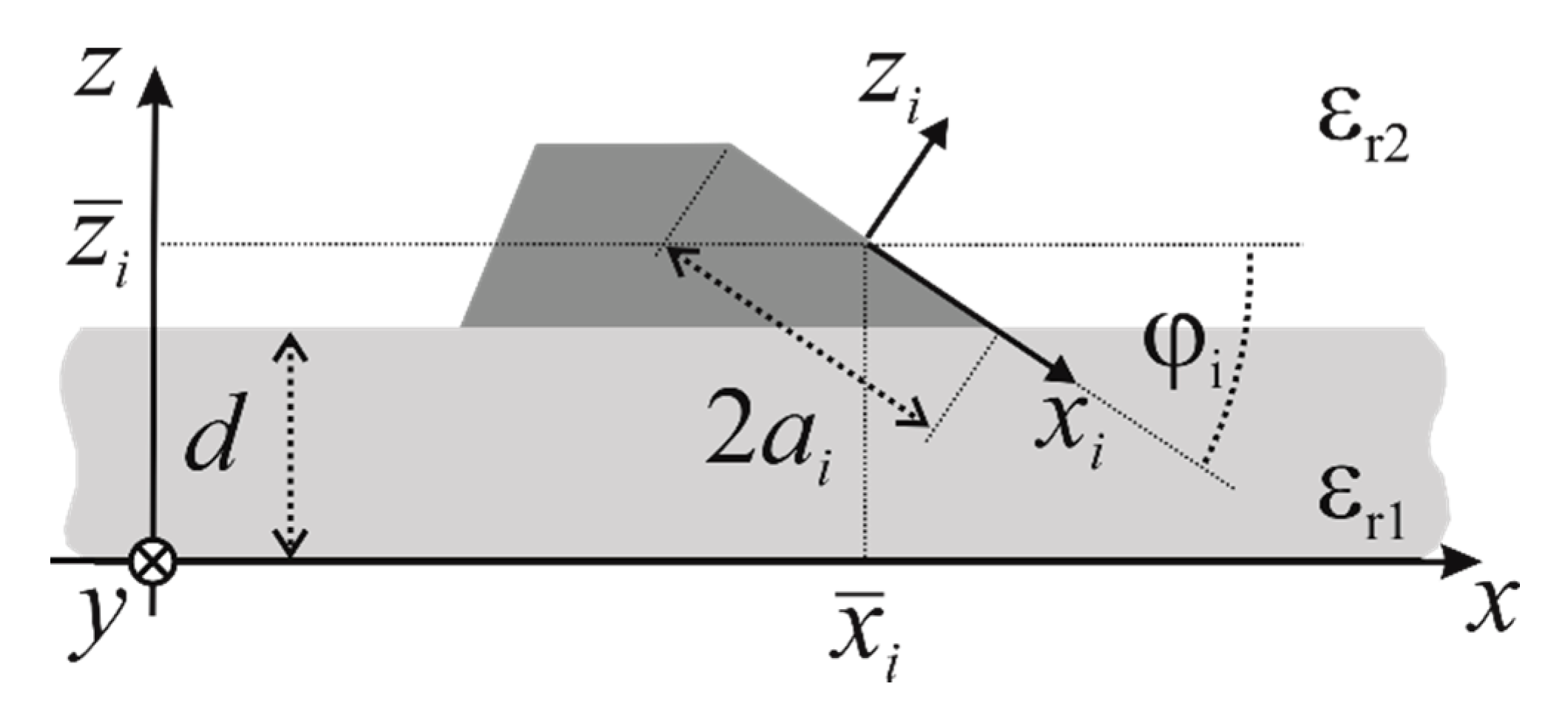
2. Background: Formulation of the Problem and Matrix Equation

Figure 1 shows the geometry of the problem in hand: a perfectly electrically conducting (PEC) polygonal cross-section strip in a homogeneous and isotropic half-space (medium 2) of relative dielectric permittivity ${\epsilon }_{r2}$ placed on a grounded planar layer (medium 1) of relative dielectric permittivity ${\epsilon }_{r1}>{\epsilon }_{r2}$ and thickness d. Thus, $k_l=k_0\sqrt{{\epsilon }_{rl}}$ with $l\in \left\{1,2\right\}$ denotes the wavenumber in medium l, where $k_0=\omega \sqrt{{\epsilon }_0{\mu }_0}=2\pi /{\lambda }_0$ is the free-space wavenumber in vacuum, $\omega$ is the angular frequency, ${\epsilon }_0$ and ${\mu }_0$ are the dielectric permittivity and the magnetic permeability of vacuum, respectively, and ${\lambda }_0$ is the wavelength in vacuum.

Let us introduce a Cartesian coordinate system $\left(x,y,z\right)$ with the origin on the ground plane, the y axis parallel to the strip axis and the z axis orthogonal to the interface between the involved media. Moreover, let us number the L sides of the strip clockwise and introduce a local Cartesian coordinate system $\left(x_i,y,z_i\right)$ on the i-th side, of length $2a_i$, with the origin at the center of the side itself in the position $\left({\overline{x}}_i,{\overline{z}}_i\right)$ with respect to the main coordinate system, such that the $z_i$ axis is orthogonal to the i-th side and oriented in the outward direction, and the angle of the $x_i$ axis with respect to the x axis is denoted by ${\phi }_i$.

The analysis of the propagation needs to assume a behavior of the fields along the y axis of the kind $e^{-jvy}$, where $v=v_R-j{v}_I$ is the mode propagation constant. According to the procedure detailed in Ref. [16], the field can be written as the superposition of the fields generated by the surface current densities on each side of the considered strip. Moreover, remembering that the edge behavior of the components of the surface current density on the i-th side is [44]

$$J_{iy}\left(x_i\right),\frac{\partial J_{i{x}_i}\left(x_i\right)}{\partial x_i}\stackrel{x_i\to \pm a_i}{\sim }{\left(1\mp \frac{x_i}{a_i}\right)}^{t_i^{\pm }-1}$$

(1)

with $t_i^{\pm }\ge 1/2$, and that the transverse component of the surface current density is continuous even on the wedges, i.e., $C_i=J_{q{x}_q}\left(a_q\right)=J_{i{x}_i}\left(-a_i\right)$, where q and i denote two consecutive sides, the following spectral domain integral representation for the longitudinal and the transverse components of the electric field in the upper half-space can be established [16]:

$$E_s\left(x,y,z\right)=E_s^t\left(x,y,z\right)+E_s^y\left(x,y,z\right)$$

(2)

with $s\in \left\{x_j,y\right\}$, and the superscripts t and y denote the functional dependence on the transverse current and the longitudinal current, respectively, where

$$E_s^r\left(x,y,z\right)=j\frac{e^{-jvy}}{2\omega {\epsilon }_0{\epsilon }_{r2}}\left[{\overline{E}}_{s,P}^r\left(x,y,z\right)+{\overline{E}}_{s,S}^r\left(x,y,z\right)\right]$$

(3)

with $r\in \left\{t,y\right\}$, and P and S denote the primary (free-space) contribution and the scattered contribution (due to the dielectric slab and the ground plane), respectively,

$$\begin{array}{l}{\overline{E}}_{x_j,P}^t\left(x,y,z\right)={\displaystyle \sum _{i=1}^L\{\frac{C_i}{2\pi j}{\displaystyle \underset{C}{\int }\left[\frac{F_{q,j}\left(u,x,z\right)}{e^{-ju{a}_q}}-\frac{F_{i,j}\left(u,x,z\right)}{e^{ju{a}_i}}\right]du}+}\\ +{\displaystyle \underset{C}{\int }{U}_{i,j}\left(u,x,z\right){\overline{J}}_{i{x}_i}\left(u\right)V_i\left(u,x,z\right)du}\}\end{array}$$

(4a)

$${\overline{E}}_{x_j,P}^y\left(x,y,z\right)={\displaystyle \sum _{i=1}^L{\displaystyle \underset{C}{\int }v{T}_{i,j}\left(u,x,z\right){\tilde{J}}_{iy}\left(u\right)V_i\left(u,x,z\right)du}},$$

(4b)

$$\begin{array}{l}{\overline{E}}_{y,P}^t\left(x,y,z\right)={\displaystyle \sum _{i=1}^L\{\frac{C_i}{2\pi j}{\displaystyle \underset{C}{\int }\left[\frac{V_q\left(u,x,z\right)}{e^{-ju{a}_q}}-\frac{V_i\left(u,x,z\right)}{e^{ju{a}_i}}\right]vdu}+}\\ +{\displaystyle \underset{C}{\int }uv{\overline{J}}_{i{x}_i}\left(u\right)V_i\left(u,x,z\right)du}\}\end{array}$$

(4c)

$${\overline{E}}_{y,P}^y\left(x,y,z\right)={\displaystyle \sum _{i=1}^L{\displaystyle \underset{C}{\int }\left(v^2-k_2^2\right){\tilde{J}}_{iy}\left(u\right)V_i\left(u,x,z\right)du}},$$

(4d)

$$\begin{array}{l}{\overline{E}}_{x_j,S}^t\left(x,y,z\right)={\displaystyle \sum _{i=1}^L\{\frac{C_i}{2\pi j}{\displaystyle \underset{C}{\int }\left[\frac{G_{q,j}^{\left(1,1\right)}\left(u\right)}{S_q\left(u\right)}-\frac{G_{i,j}^{\left(1,1\right)}\left(u\right)}{S_i\left(u\right)}\right]\frac{W_i\left(u,x,z\right)}{e^{j{S}_i\left(u\right)a_i}}du}+}\\ \begin{array}{cc}& \end{array}+{\displaystyle \underset{C}{\int }{G}_{i,j}^{\left(1,1\right)}\left(u\right){\overline{J}}_{i{x}_i}\left(S_i\left(u\right)\right)W_i\left(u,x,z\right)du}\}\end{array}$$

(4e)

$${\overline{E}}_{x_j,S}^y\left(x,y,z\right)={\displaystyle \sum _{i=1}^L{\displaystyle \underset{C}{\int }{G}_j^{\left(1,2\right)}\left(u\right){\tilde{J}}_{iy}\left(S_i\left(u\right)\right)W_i\left(u,x,z\right)du}},$$

(4f)

$$\begin{array}{l}{\overline{E}}_{y,S}^t\left(x,y,z\right)={\displaystyle \sum _{i=1}^L\{\frac{C_i}{2\pi j}{\displaystyle \underset{C}{\int }\left[\frac{G_q^{\left(2,1\right)}\left(u\right)}{S_q\left(u\right)}-\frac{G_i^{\left(2,1\right)}\left(u\right)}{S_i\left(u\right)}\right]\frac{W_i\left(u,x,z\right)}{e^{j{S}_i\left(u\right)a_i}}du}+}\\ \begin{array}{cc}& \end{array}+{\displaystyle \underset{C}{\int }{G}_i^{\left(2,1\right)}\left(u\right){\overline{J}}_{i{x}_i}\left(S_i\left(u\right)\right)W_i\left(u,x,z\right)du}\}\end{array}$$

(4g)

$${\overline{E}}_{y,S}^y\left(x,y,z\right)={\displaystyle \sum _{i=1}^L{\displaystyle \underset{C}{\int }{G}^{\left(2,2\right)}\left(u\right){\tilde{J}}_{iy}\left(S_i\left(u\right)\right)W_i\left(u,x,z\right)du}},$$

(4h)

C denotes the selected inverse Fourier transform integration path in the complex plane $u=u_R+j{u}_I$, ${\underset{\_}{\tilde{J}}}_i\left(u\right)$ is the Fourier transform of the current on the i-th side with respect to $x_i$, ${\overline{J}}_{i{x}_i}\left(u\right)={\tilde{J}}_{i{x}_i}\left(u\right)-{\tilde{J}}_{i{x}_i}^{\infty }\left(u\right)$, ${\tilde{J}}_{i{x}_i}^{\infty }\left(u\right)=\left(-C_i{e}^{-ju{a}_i}+C_p{e}^{ju{a}_i}\right)/\left(2\pi ju\right)$, q, i and p denote three consecutive sides, and the kernels are summarized in the Appendix A.

As such, by forcing the tangential components of the electric field to be zero on the strip surface, a homogeneous EFIE in the spectral domain is obtained

$${E_s\left(x,y,z\right)|}_{\left|x_j\right|\le a_j,z_j=0}=0$$

(5)

with $s\in \left\{x_j,y\right\}$ and $j=1,2,\dots L$.

In order to guarantee fast convergence, the Galerkin method, with the expansion functions introduced in Ref. [27], reconstructing the physical properties of the fields even on the wedges of the PEC strip, is used to discretize the equation in (5). The Fourier transforms of the selected expansion functions can be expressed in closed form as [27]

$${\tilde{\varphi }}_{-1}^{\left(\alpha ,\beta \right)}\left(au\right)=\frac{e^{jua}-e^{-jua}{}_{1}F_1\left(\beta ;\alpha +\beta ;j2ua\right)}{2j\pi u}$$

(6a)

$${\tilde{\varphi }}_n^{\left(\alpha ,\beta \right)}\left(au\right)={\overline{\xi }}_n^{(\alpha ,\beta )}{\left(2jua\right)}^n{e}^{-jua}{}_{1}F_1\left(n+\beta +1;2n+\alpha +\beta +2;2jua\right)$$

(6b)

$${\overline{\xi }}_n^{(\alpha ,\beta )}=\sqrt{\frac{a{2}^{\alpha +\beta -1}\Gamma \left(n+\alpha +1\right)\Gamma \left(n+\beta +1\right)\Gamma \left(n+\alpha +\beta +1\right)}{{\pi }^{2}n!\Gamma \left(2n+\alpha +\beta +1\right)\Gamma \left(2n+\alpha +\beta +2\right)}}$$

(6c)

where the symbol ${}_{1}F_1\left(\cdot ;\cdot ;\cdot \right)$ denotes the CHF1 and $\Gamma (\cdot )$ is the Gamma function [45]. On the basis of this property and the reciprocity theorem, it is not difficult to demonstrate that the convolution integrals resulting from Galerkin projection can be reduced to algebraic products [16]. As such, the elements of the obtained matrix equation can be expressed as linear combinations of one-dimensional integrals over the selected inverse Fourier transform integration path.

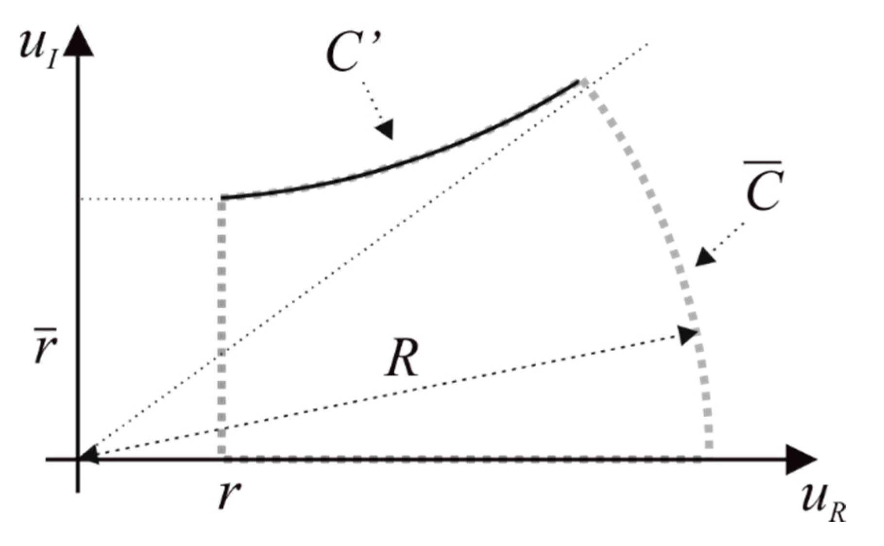
3. Fast Evaluation of the Matrix Coefficients

For $n,m\ge 0$, the general integral associated with the primary contribution can be written as

$$I_P={\displaystyle \underset{C}{\int }{f}_i\left(u,{\overline{x}}_j,{\overline{z}}_j\right){\tilde{\varphi }}_n^{\left({\alpha }_i,{\beta }_i\right)}\left(a_{i}u\right){\tilde{\varphi }}_m^{\left({\alpha }_j,{\beta }_j\right)}\left(-a_j{\left[T_{i,j}\left(u,{\overline{x}}_j,{\overline{z}}_j\right)\right]}^{\ast }\right)du}$$

(7)

where $f_i\left(u,{\overline{x}}_j,{\overline{z}}_j\right)$ is one of the kernels in Equations (4a)–(4d), $T_{i,j}\left(u,{\overline{x}}_j,{\overline{z}}_j\right)$ is defined in Equation (A1f), and the star denotes the complex conjugate of a complex number, while the general integral associated to the scattered contribution is

$$I_S=I_S^{\prime }+I_S^{″}$$

(8a)

$$I_S^{\prime }={\displaystyle \underset{C}{\int }\left[g_i\left(u,{\overline{x}}_j,{\overline{z}}_j\right)-g_i^{\infty }\left(u,{\overline{x}}_j,{\overline{z}}_j\right)\right]{\tilde{\varphi }}_n^{\left({\alpha }_i,{\beta }_i\right)}\left(a_i{S}_i\left(u\right)\right){\tilde{\varphi }}_m^{\left({\alpha }_j,{\beta }_j\right)}\left(-a_j{\left[S_j\left(u\right)\right]}^{\ast }\right)du}$$

(8b)

$$I_S^{″}={\displaystyle \underset{C}{\int }{g}_i^{\infty }\left(u,{\overline{x}}_j,{\overline{z}}_j\right){\tilde{\varphi }}_n^{\left({\alpha }_i,{\beta }_i\right)}\left(a_i{S}_i\left(u\right)\right){\tilde{\varphi }}_m^{\left({\alpha }_j,{\beta }_j\right)}\left(-a_j{\left[S_j\left(u\right)\right]}^{\ast }\right)du}$$

(8c)

where $g_i\left(u,{\overline{x}}_j,{\overline{z}}_j\right)$ is one of the kernels in Equations (4e)–(4h), $g_i^{\infty }\left(u,{\overline{x}}_j,{\overline{z}}_j\right)$ is obtained starting from $g_i\left(u,{\overline{x}}_j,{\overline{z}}_j\right)$ by replacing $C_K\left(u\right)$ for $K\in \left\{E,H\right\}$, defined in Equations (A1m) and (A1n), respectively, with $C_K^{\infty }\left(u\right)=\underset{d\to +\infty }{\lim }{C}_K\left(u\right)$, and $S_j\left(u\right)$ is defined in Equation (A1p). Since the coefficient matrix elements for $n=-1$ and/or $m=-1$ can be written in a similar way, they are here omitted for the sake of brevity.

The integrals in Equations (7), (8b) and (8c) are improper integrals. According to the asymptotic behavior for the large argument of the CHF1 [45], i.e.,

$${}_{1}F_1\left(a;b;u\right)\stackrel{\left|u\right|\to +\infty }{\sim }\frac{e^{\pm j\pi a}{u}^{-a}\Gamma \left(b\right)}{\Gamma \left(b-a\right)}+\frac{e^u{u}^{a-b}\Gamma \left(b\right)}{\Gamma \left(a\right)}$$

(9)

where the upper sign has to be chosen for $-\pi /2\le \arg (u)<3\pi /2$ and the lower sign for $-3\pi /2<\arg (u)\le \pi /2$, and observing that $C_K\left(u\right)-C_K^{\infty }\left(u\right)\stackrel{\left|u\right|\to +\infty }{\sim }{e}^{-2\left|u\right|d}$, it can be concluded that the integrand of the integral in Equation (8b) has an asymptotic exponential decay, while the integrals in Equations (7) and (8c) involve asymptotically oscillating functions with an algebraic decay in the worst cases. As a result, the numerical evaluation of such kinds of integrals is less and less efficient as the accuracy required for the solution is higher. The asymptotic decay of the integrands in Equations (7) and (8c) can be sped up by pulling out the asymptotic behavior of the integrand such that the integrals of the extracted contributions can be expressed in closed form. Nevertheless, such a procedure does not change the oscillating nature of the integrands, which keep on having an algebraic decay. Therefore, the numerical convergence of the accelerated integrals, even if faster, is still strongly dependent on the accuracy required for the solution.

A new procedure, overcoming this problem, is shown in the following. For the sake of brevity, only the integrals associated to the primary contribution for $n,m\ge 0$ and the propagation of bound modes are considered, the generalization of the proposed technique to the other cases being straightforward. For bound modes propagation, the propagation constant is real, i.e., $v=v_R$, and such that $k_2<v_R<k_1$; therefore, the square-roots branch points of the free-space Green’s function in the spectral domain are imaginary numbers. Let us assume the real axis of the complex plane u as the inverse Fourier transform integration path C.

As a first task, observing that the CHF1 can be written as [45]

$${}_{1}F_1\left(a;b;u\right)=\frac{\Gamma \left(b\right)e^{\pm j\pi a}}{\Gamma \left(b-a\right)}U\left(a;b;u\right)+\frac{\Gamma \left(b\right)e^u{e}^{\mp j\pi \left(b-a\right)}}{\Gamma \left(a\right)}U\left(b-a;b;-u\right)$$

(10)

where $U\left(\cdot ;\cdot ;\cdot \right)$ denotes the CHF2 [45], the upper sign has to be chosen for $-\pi /2\le \arg (u)<3\pi /2$ and the lower sign for $-3\pi /2<\arg (u)\le \pi /2$, the following alternative expression for the expansion functions in the spectral domain defined in Equation (6b) can be introduced:

$${\tilde{\varphi }}_n^{\left(\alpha ,\beta \right)}\left(u\right)={\tilde{\psi }}_n^{\left(\alpha ,\beta \right)}\left(u\right)+{\left(-1\right)}^n{\tilde{\psi }}_n^{\left(\beta ,\alpha \right)}\left(-u\right)$$

(11)

where

$${\tilde{\psi }}_n^{\left(\alpha ,\beta \right)}\left(u\right)=\frac{{\overline{\xi }}_n^{(\alpha ,\beta )}\Gamma \left(2n+\alpha +\beta +1\right)}{\Gamma \left(n+\alpha +1\right)}{e}^{\pm j\pi \left(n+\beta +1\right)}{\left(2ju\right)}^n{e}^{-jz}U\left(n+\beta +1;2n+\alpha +\beta +2;2ju\right)$$

(12)

the upper sign has to be chosen for $-\pi /2<\arg (u)\le \pi /2$ and the lower sign for $\pi /2<\arg (u)\le 3\pi /2$.

The properties of the function in Equation (12) can be immediately deduced from the following relation between the CHF1 and the CHF2 [45]:

$$U(a,b,u)=\frac{\pi }{\sin \left(\pi b\right)}\left[\frac{{}_1{F}_1(a,b,u)}{\Gamma \left(1+a-b\right)\Gamma \left(b\right)}-u^{1-b}\frac{{}_1{F}_1(1+a-b,2-b,u)}{\Gamma \left(a\right)\Gamma \left(2-b\right)}\right]$$

(13)

As such, ${\tilde{\psi }}_n^{\left(\alpha ,\beta \right)}\left(u\right)$ is a many-valued function if $\alpha +\beta$ is a non-integer number with a branch-cut for $u_R=0$ and $u_I>0$, and is singular for $u=0$ except when $\alpha =\beta =-1/2$ and $n=0$ simultaneously.

Let us introduce the auxiliary function:

$$\begin{array}{l}{\overline{F}}_{n,m,w,s,t}^{\left(i,j\right)}\left(u\right)={\left(-1\right)}^{ns+mt}{f}_i\left({\left(-1\right)}^{w}u,{\overline{x}}_j,{\overline{z}}_j\right)\cdot \\ \cdot {\tilde{\psi }}_n^{\left(t_i^{\left(s\right)},t_i^{\left(\left|s-1\right|\right)}\right)}\left({\left(-1\right)}^{w+s}{a}_{i}u\right){\tilde{\psi }}_m^{\left(t_j^{\left(t\right)},t_j^{\left(\left|t-1\right|\right)}\right)}\left(-{\left(-1\right)}^t{a}_j{\left[T_{i,j}\left({\left(-1\right)}^{w}u,{\overline{x}}_j,{\overline{z}}_j\right)\right]}^{*}\right)\end{array}$$

(14)

where $w,s,t\in \left\{0,1\right\}$, $t_l^{\left(0\right)}={\alpha }_l$ and $t_l^{\left(1\right)}={\beta }_l$, with $l\in \left\{i,j\right\}$. Such a function is generally a many-valued function with two extra branch-cuts associated with the involved CHF2. The first one is along the imaginary axis of the complex plane u ($u_R=0$) with a branch point at $u=0$, while the second one lies on the hyperbole described by the equation $s_{i,j}^2{u}_R^2-c_{i,j}^2{u}_I^2+s_{i,j}^2{c}_{i,j}^2\left(v_R^2-k_2^2\right)=0$, where $s_{i,j}$ and $c_{i,j}$ are defined in the Appendix A, with a branch point at $u=-j\mathrm{sgn}\left(z_i\left(x,z\right)\right)s_{i,j}\sqrt{v_R^2-k_2^2}$.

By setting

$$F_{n,m}^{\left(i,j\right)}\left(u\right)=f_i\left(u,{\overline{x}}_j,{\overline{z}}_j\right){\tilde{\varphi }}_n^{\left({\alpha }_i,{\beta }_i\right)}\left(a_{i}u\right){\tilde{\varphi }}_m^{\left({\alpha }_j,{\beta }_j\right)}\left(-a_j{\left[T_{i,j}\left(u,{\overline{x}}_j,{\overline{z}}_j\right)\right]}^{\ast }\right)$$

(15)

the following new representation for the integral in Equation (7) can be immediately stated

$${\displaystyle \underset{-\infty }{\overset{+\infty }{\int }}{F}_{n,m}^{\left(i,j\right)}\left(u\right)du}={\displaystyle \underset{-r}{\overset{r}{\int }}{F}_{n,m}^{\left(i,j\right)}\left(u\right)du}+{\displaystyle \sum _{w,s,t=0}^1{\displaystyle \underset{r}{\overset{+\infty }{\int }}{\overline{F}}_{n,m,w,s,t}^{\left(i,j\right)}\left(u\right)du}}$$

(16)

where $r>0$ in order to avoid the singularity of ${\overline{F}}_{n,m,w,s,t}^{\left(i,j\right)}\left(u\right)$ for $u=0$.

The asymptotic behavior for the large argument of the CHF2, i.e., [45]

$$U\left(a;b;u\right)\stackrel{\left|u\right|\to +\infty }{\sim }{u}^{-a}$$

(17)

for $-3\pi /2<\arg (u)<3\pi /2$, allows us to obtain the following representation for the function in Equation (14) on its principal sheet:

$${\overline{F}}_{n,m,w,s,t}^{\left(i,j\right)}\left(u\right)={\widehat{F}}_{n,m,w,s,t}^{\left(i,j\right)}\left(u\right)e^{G_{w,s,t}^{\left(i,j\right)}\left(u\right)}$$

(18)

where ${\widehat{F}}_{n,m,w,s,t}^{\left(i,j\right)}\left(u\right)$ is a non-oscillating function with an asymptotic algebraic decay of the kind $1/u^{\gamma }$ with $\gamma \ge 2$,

$$G_{w,s,t}^{\left(i,j\right)}\left(u\right)=j{\alpha }_{w,s,t}^{\left(i.j\right)}u-{\beta }_t^{\left(i,j\right)}{R}_2\left(u\right)$$

(19a)

$${\alpha }_{w,s,t}^{\left(i,j\right)}={\left(-1\right)}^w\left[-{\left(-1\right)}^s{a}_i+{\left(-1\right)}^t{a}_j{c}_{i,j}-x_i\left({\overline{x}}_j,{\overline{z}}_j\right)\right]$$

(19b)

$${\beta }_t^{\left(i,j\right)}={\left(-1\right)}^t{a}_j\mathrm{sgn}\left(z_i\left({\overline{x}}_j,{\overline{z}}_j\right)\right)s_{i,j}+\left|z_i\left({\overline{x}}_j,{\overline{z}}_j\right)\right|$$

(19c)

where $R_2\left(u\right)$ is defined in Equation (A1r), and it is simple to observe that ${\beta }_t^{\left(i,j\right)}\ge 0$.

The condition

$$\Im \left\{G_{w,s,t}^{\left(i,j\right)}\left(u\right)\right\}=0\iff {\widehat{s}}^2{u}_R^2-{\widehat{c}}^2{u}_I^2+{\widehat{s}}^2{\widehat{c}}^2\left(v_R^2-k_2^2\right)=0$$

(20)

where $\Im \{\cdot \}$ denotes the imaginary part of a complex number and the quantities $\widehat{s}={\alpha }_{s,t}^{\left(i,j\right)}/\sqrt{{\left({\alpha }_{s,t}^{\left(i,j\right)}\right)}^2+{\left({\beta }_t^{\left(i,j\right)}\right)}^2}$ and $\widehat{c}={\beta }_t^{\left(i,j\right)}/\sqrt{{\left({\alpha }_{s,t}^{\left(i,j\right)}\right)}^2+{\left({\beta }_t^{\left(i,j\right)}\right)}^2}$ have been introduced for the sake of the simplicity of notation, identifies the path along which ${\overline{F}}_{n,m,w,s,t}^{\left(i,j\right)}\left(u\right)$ does not oscillate. On the other hand, assuming the condition (20), the integrability of ${\overline{F}}_{n,m,w,s,t}^{\left(i,j\right)}\left(u\right)$ is guaranteed by the extra condition

$$\Re \left\{G_{w,s,t}^{\left(i,j\right)}\left(u\right)\right\}\le 0\iff \mathrm{sgn}\left(\widehat{s}\right)u_I\ge 0$$

(21)

where $\Re \{\cdot \}$ denotes the real part of a complex number.

To conclude, we can simply demonstrate that the general improper integral at the right-hand side of Equation (16) can be expressed as a combination of a proper integral and an improper integral of a non-oscillating function by means of the Cauchy’s integral theorem and the Jordan’s lemma. Indeed, supposing, just for an example, that $0\le \widehat{s}<\left|s_{i,j}\right|$, due to the properties of ${\overline{F}}_{n,m,w,s,t}^{\left(i,j\right)}\left(u\right)$ detailed above, it is simple to state that

$$\underset{R\to \infty }{\lim }{\displaystyle \underset{\overline{C}}{\oint }{\overline{F}}_{n,m,w,s,t}^{\left(i,j\right)}\left(u\right)du}=0\iff {\displaystyle \underset{r}{\overset{+\infty }{\int }}{\overline{F}}_{n,m,w,s,t}^{\left(i,j\right)}\left(u\right)du}={\displaystyle \underset{r}{\overset{r+j\overline{r}}{\int }}{\overline{F}}_{n,m,w,s,t}^{\left(i,j\right)}\left(u\right)du}+{\displaystyle \underset{C^{\prime }}{\int }{\overline{F}}_{n,m,w,s,t}^{\left(i,j\right)}\left(u\right)du}$$

(22)

where $\overline{C}$ is the dotted gray closed contour defined in Figure 2, $C^{\prime }$ (the black solid line in Figure 2) is the integration path defined by the Equations in (20) and (21) along with the function ${\overline{F}}_{n,m,w,s,t}^{\left(i,j\right)}\left(u\right)$ does not oscillate, and $\left(r,\overline{r}\right)$ denotes the intersection point between the path $C^{\prime }$ and the straight line $u=r$.

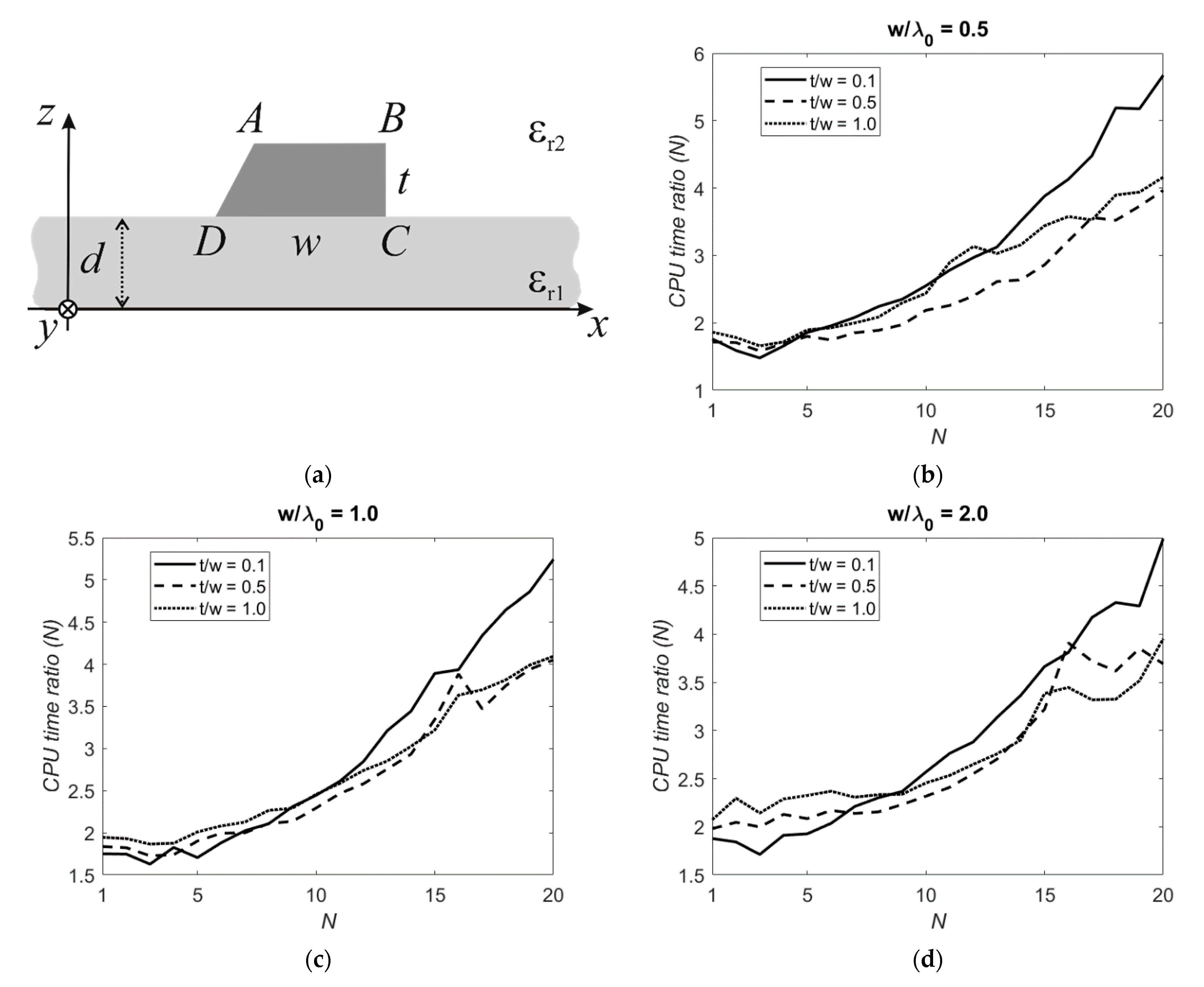
4. Numerical Results and Discussion

An approximation of the mode propagation constants can be obtained by searching for the nulls of the determinant of the truncated matrix equation. In Ref. [16], following this line of reasoning, the effectiveness of the discretization scheme presented in Section 2 has been widely demonstrated. Indeed, few expansion functions have been needed to achieve accurate solutions for both bound and leaky mode propagations. As such, in order to avoid unnecessary repetitions, no details are given in this section about the convergence of the method and the comparisons with the literature. Instead, this section is aimed at showing that the procedure detailed in Section 3 always outperforms the classical analytical asymptotic acceleration technique used in Ref. [16] in terms of computation time.

Let us define the CPU time ratio as the ratio between the computation time needed to fill the coefficient matrix as obtained by using the analytical asymptotic acceleration technique with respect to the technique detailed above. The simulations are performed on a laptop equipped with an Intel Core I7-10510U 1.80 GHz–2.30 GHz, 16 GB RAM, running Windows 10 Home 64 bit and the integrals are evaluated by means of an adaptive Gaussian quadrature routine.

The geometry of the examined problem is sketched in Figure 3a: a general trapezoidal cross-section strip in vacuum (${\epsilon }_{r2}=1$) with $\overline{AB}=3w/4$, $\overline{BC}=t$, $\overline{CD}=w$ and $\widehat{B}=\widehat{C}=\pi /2$ on a grounded dielectric layer of thickness $d=0.2117{\lambda }_0$ and a relative dielectric permittivity ${\epsilon }_{r1}=9.8$. We assume $v_R/k_0=1.5$, $w/{\lambda }_0=0.5,1.0,2.0$ and $t/w=0.1,0.5,1.0$ as test cases and set the accuracy of the quadrature routine in such a way as to guarantee the convergence of six significant digits in the numerical evaluation of the integrals. As can be clearly deduced by inspecting Figure 3b–d, where the CPU time ratio is plotted as a function of the number of expansion functions used for each component of the surface current density on each side (N), the technique proposed in this paper always outperforms the classical analytical asymptotic acceleration technique. Moreover, the proposed results clearly show that the CPU time ratio is substantially independent of the size of the strip with respect to the wavelength and of the shape of the strip, thus demonstrating the effectiveness of the proposed technique. It is important to note that the CPU time ratio dramatically increases as the number of expansion functions used becomes higher. At the same time, for a given number of expansion functions used, the CPU time ratio increases as the accuracy set for the quadrature routine becomes higher. Indeed, in spite of what happens for the improper integrals of asymptotically oscillating functions, the computation time of the new representation of the coefficient matrix elements is weakly affected by the accuracy required for the numerical evaluation of the integrals. Just for an example, for $w/{\lambda }_0=1.0$, $t/w=0.5$ and $N=20$, the proposed method is four time faster than the analytical asymptotic acceleration technique (see Figure 3c). However, for the same case, the CPU time ratio becomes 7 when the convergence of 8 significant digits in the numerical evaluation of the integrals is required, and even reaches 18 for 10 significant digits of accuracy. Moreover, it is worth noting that this exponential behavior is confirmed also for the other cases examined in Figure 3b–d. To conclude, the technique presented in this paper is particularly advantageous when highly accurate results are searched for.

5. Conclusions

Fast convergence was achieved in Ref. [16] by applying the MAP to an integral equation formulation in the spectral domain for the analysis of the propagation in polygonal cross-section microstrip lines. In this paper, the technique proposed in Ref. [16] has been improved by devising a new expression for the coefficient matrix elements, leading to a drastic reduction in the computation time. It is worth observing that the line of reasoning proposed in this paper is versatile, and can be applied to a wide class of problems formulated in the spectral domain and discretized by means of MAP. On the other hand, a specific procedure has to be conceived for the particular problem in hand, which can be seen as the only limitation to the proposed approach. Particularly attractive is the application of the proposed technique to the analysis of the radiation characteristics of a microstrip antenna array, because the integrands of the integrals of mutual contributions between two antennas oscillate faster as the distance between the antennas increases. Moreover, the method can be readily generalized to the analysis of the propagation in polygonal cross-section optical waveguides.

References

1. Michalski, K.A.; Zheng, D. Rigorous analysis of open microstrip lines of arbitrary cross section in bound and leaky regimes. IEEE Trans. Microw. Theory Tech. 1989, 37, 2005–2010. [Google Scholar] [CrossRef]
2. Zhu, L.; Yamashita, E. New method for the analysis of dispersion characteristics of various planar transmission lines with finite metallization thickness. IEEE Microw. Guided Wave Lett. 1991, 1, 164–166. [Google Scholar] [CrossRef]
3. Hsu, C.-I.G.; Harrington, R.F.; Michalski, K.A.; Zheng, D. Analysis of multiconductor transmission lines of arbitrary cross section in multilayered uniaxial media. IEEE Trans. Microw. Theory Tech. 1993, 41, 70–78. [Google Scholar] [CrossRef]
4. Olyslager, F.; De Zutter, D.; Blomme, K. Rigorous analysis of the propagation characteristics of general lossless and lossy muticonductor transmission lines in multilayered media. IEEE Trans. Microw. Theory Tech. 1993, 41, 79–88. [Google Scholar] [CrossRef] [Green Version]
5. Bernal, J.; Medina, F.; Boix, R.R. Full-wave analysis of nonplanar transmission lines on layered medium by means of MPIE and complex image theory. IEEE Trans. Microw. Theory Tech. 2001, 49, 177–185. [Google Scholar] [CrossRef]
6. Bernal, J.; Mesa, F.; Medina, F. 2-D analysis of leakage in printed-circuit lines using discrete complex-images technique. IEEE Trans. Microw. Theory Tech. 2002, 50, 1895–1900. [Google Scholar] [CrossRef]
7. Chen, H.H. Finite-element method coupled with method of lines for the analysis of planar or quasi-planar transmission lines. IEEE Trans. Microw. Theory Tech. 2003, 51, 848–855. [Google Scholar] [CrossRef]
8. Su, K.Y.; Kuo, J.T. An efficient analysis of shielded single and multiple coupled microstrip lines with the nonuniform fast Fourier transform (NUFFT) technique. IEEE Trans. Microw. Theory Tech. 2004, 52, 90–96. [Google Scholar] [CrossRef]
9. Hwang, J.-N. A compact 2-D FDFD method for modeling microstrip structures with nonuniform grids and perfectly matched layer. IEEE Trans. Microw. Theory Tech. 2005, 53, 653–659. [Google Scholar] [CrossRef]
10. Tong, M.; Pan, G.; Lei, G. Full-wave analysis of coupled lossy transmission lines using multiwavelet-based method of moments. IEEE Trans. Microw. Theory Tech. 2005, 53, 2362–2370. [Google Scholar] [CrossRef]
11. Migliore, M.D.; Pinchera, D.; Lucido, M.; Schettino, F.; Panariello, G. A sparse recovery approach for pattern correction of active arrays in presence of element failures. IEEE Antennas Wirel. Propag. Lett. 2015, 14, 1027–1030. [Google Scholar] [CrossRef]
12. Pinchera, D.; Migliore, M.D.; Lucido, M.; Schettino, F.; Panariello, G. A compressive-sensing inspired alternate projection algorithm for sparse array synthesis. Electronics 2017, 6, 3. [Google Scholar] [CrossRef] [Green Version]
13. Tsalamengas, J.L. Quadrature rules for weakly singular, strongly singular, and hypersingular integrals in boundary integral equation methods. J. Comput. Phys. 2015, 303, 498–513. [Google Scholar] [CrossRef]
14. Bulygin, V.S.; Gandel, Y.V.; Nosich, A.I. Nystrom-type method in three-dimensional electromagnetic diffraction by a finite PEC rotationally symmetric surface. IEEE Trans. Antennas Propag. 2012, 60, 4710–4718. [Google Scholar] [CrossRef]
15. Muller, C. Foundations of the Mathematical Theory of Electromagnetic Waves; Springer: Berlin, Germany, 1969. [Google Scholar]
16. Coluccini, G.; Lucido, M.; Panariello, G. Spectral domain analysis of open single and coupled microstrip lines with polygonal cross-section in bound and leaky regimes. IEEE Trans. Microw. Theory Tech. 2013, 61, 736–745. [Google Scholar] [CrossRef]
17. Hongo, K. Diffraction by a flanged parallel-plate waveguide. Radio Sci. 1972, 7, 955–963. [Google Scholar] [CrossRef]
18. Hongo, K.; Ishii, G. Diffraction of an electromagnetic plane wave by a thick slit. IEEE Trans. Antennas Propag. 1978, 26, 494–499. [Google Scholar] [CrossRef]
19. Eswaran, K. On the solutions of a class of dual integral equations occurring in diffraction problems. Proc. R. Soc. Lond. Ser. A 1990, 429, 399–427. [Google Scholar]
20. Veliev, E.I.; Veremey, V.V. Numerical-analytical approach for the solution to the wave scattering by polygonal cylinders and flat strip structures. In Analytical and Numerical Methods in Electromagnetic Wave Theory; Hashimoto, M., Idemen, M., Tretyakov, O.A., Eds.; Science House: Tokyo, Japan, 1993; pp. 470–514. [Google Scholar]
21. Davis, M.J.; Scharstein, R.W. Electromagnetic plane wave excitation of an open-ended finite-length conducting cylinder. J. Electromagn. Waves Appl. 1993, 7, 301–319. [Google Scholar] [CrossRef]
22. Hongo, K.; Serizawa, H. Diffraction of electromagnetic plane wave by rectangular plate and rectangular hole in the conducting plate. IEEE Trans. Antennas Propag. 1999, 47, 1029–1041. [Google Scholar] [CrossRef]
23. Bliznyuk, N.Y.; Nosich, A.I.; Khizhnyak, A.N. Accurate computation of a circular-disk printed antenna axisymmetrically excited by an electric dipole. Microw. Opt. Technol. Lett. 2000, 25, 211–216. [Google Scholar] [CrossRef]
24. Tsalamengas, J.L. Rapidly converging direct singular integral-equation techniques in the analysis of open microstrip lines on layered substrates. IEEE Trans. Microw. Theory Tech. 2001, 49, 555–559. [Google Scholar] [CrossRef]
25. Losada, V.; Boix, R.R.; Medina, F. Fast and accurate algorithm for the short-pulse electromagnetic scattering from conducting circular plates buried inside a lossy dispersive half-space. IEEE Trans. Geosci. Remote Sens. 2003, 41, 988–997. [Google Scholar] [CrossRef]
26. Hongo, K.; Naqvi, Q.A. Diffraction of electromagnetic wave by disk and circular hole in a perfectly conducting plane. Prog. Electromagn. Res. 2007, 68, 113–150. [Google Scholar] [CrossRef] [Green Version]
27. Lucido, M.; Panariello, G.; Schettino, F. Electromagnetic scattering by multiple perfectly conducting arbitrary polygonal cylinders. IEEE Trans. Antennas Propag. 2008, 56, 425–436. [Google Scholar] [CrossRef]
28. Lucido, M.; Panariello, G.; Schettino, F. TE scattering by arbitrarily connected conducting strips. IEEE Trans. Antennas Propag. 2009, 57, 2212–2216. [Google Scholar] [CrossRef]
29. Coluccini, G.; Lucido, M.; Panariello, G. TM scattering by perfectly conducting polygonal cross-section cylinders: A new surface current density expansion retaining up to the second-order edge behavior. IEEE Trans. Antennas Propag. 2012, 60, 407–412. [Google Scholar] [CrossRef]
30. Lucido, M.; Migliore, M.D.; Pinchera, D. A new analytically regularizing method for the analysis of the scattering by a hollow finite-length PEC circular cylinder. Prog. Electromagn. Res. B 2016, 70, 55–71. [Google Scholar] [CrossRef] [Green Version]
31. Nosich, A.I. Method of analytical regularization in computational photonics. Radio Sci. 2016, 51, 1421–1430. [Google Scholar] [CrossRef]
32. Steinberg, S. Meromorphic families of compact operators. Arch. Ration. Mech. Anal. 1968, 31, 372–379. [Google Scholar] [CrossRef]
33. Park, S.; Balanis, C.A. Dispersion characteristics of open microstrip lines using closed-form asymptotic extraction. IEEE Trans. Microw. Theory Tech. 1997, 45, 458–460. [Google Scholar] [CrossRef]
34. Park, S.; Balanis, C.A. Closed-form asymptotic extraction method for coupled microstrip lines. IEEE Microw. Guided Wave Lett. 1997, 7, 84–86. [Google Scholar] [CrossRef] [Green Version]
35. Amari, S.; Vahldieck, R.; Bornemann, J. Using selective asymptotics to accelerate dispersion analysis of microstrip lines. IEEE Trans. Microw. Theory Tech. 1998, 46, 1024–1027. [Google Scholar] [CrossRef] [Green Version]
36. Lucido, M. An analytical technique to fast evaluate mutual coupling integrals in spectral domain analysis of multilayered coplanar coupled striplines. Microw. Opt. Technol. Lett. 2012, 54, 1035–1039. [Google Scholar] [CrossRef]
37. Lucido, M. A new high-efficient spectral-domain analysis of single and multiple coupled microstrip lines in planarly layered media. IEEE Trans. Microw. Theory Tech. 2012, 60, 2025–2034. [Google Scholar] [CrossRef]
38. Coluccini, G.; Lucido, M. A new high efficient analysis of the scattering by a perfectly conducting rectangular plate. IEEE Trans. Antennas Propag. 2013, 61, 2615–2622. [Google Scholar] [CrossRef]
39. Lucido, M. An efficient evaluation of the self-contribution integrals in the spectral-domain analysis of multilayered striplines. IEEE Antennas Wirel. Propag. Lett. 2013, 12, 360–363. [Google Scholar] [CrossRef]
40. Lucido, M. Complex resonances of a rectangular patch in a multilayered medium: A new accurate and efficient analytical technique. Prog. Electromagn. Res. 2014, 145, 123–132. [Google Scholar] [CrossRef] [Green Version]
41. Lucido, M. Scattering by a tilted strip buried in a lossy half-space at oblique incidence. Prog. Electromagn. Res. 2014, 37, 51–62. [Google Scholar] [CrossRef] [Green Version]
42. Lucido, M. Electromagnetic scattering by a perfectly conducting rectangular plate buried in a lossy half-space. IEEE Trans. Geosci. Remote Sens. 2014, 52, 6368–6378. [Google Scholar] [CrossRef]
43. Lucido, M.; Di Murro, F.; Panariello, G. Electromagnetic scattering from a zero-thickness PEC disk: A note on the Helmholtz-Galerkin analytically regularizing procedure. Prog. Electromagn. Res. Lett. 2017, 71, 7–13. [Google Scholar]
44. Meixner, J. The behavior of electromagnetic fields at edges. IEEE Trans. Antennas Propag. 1972, 20, 442–446. [Google Scholar] [CrossRef]
45. Abramowitz, M.; Stegun, I.A. Handbook of Mathematical Functions; Dover Publications, Inc.: New York, NY, USA, 1974. [Google Scholar]
Figure 1. Geometry of the problem.
Applsci 11 00933 g001
Figure 2. Integration paths.
Applsci 11 00933 g002
Figure 3. CPU time ratio as a function of the number of expansion functions used for each component of the surface current density on each side of the trapezoidal cross-section strip (N) with A B ¯ = 3 w / 4 , B C ¯ = t , C D ¯ = w , B ^ = C ^ = π / 2 , ε r 2 = 1 , ε r 1 = 9.8 , d = 0.2117 λ 0 , for v R / k 0 = 1.5 , w / λ 0 = 0.5 , 1.0 , 2.0 and t / w = 0.1 , 0.5 , 1.0 . (a) Geometry of the problem; (b) CPU time ration for w / λ 0 = 0.5 ; (c) CPU time ration for w / λ 0 = 1.0 ; (d) CPU time ration for w / λ 0 = 2.0 .
Applsci 11 00933 g003
Publisher’s Note: MDPI stays neutral with regard to jurisdictional claims in published maps and institutional affiliations.