Numerical Modeling of Nonlinear Response of Seafloor Porous Saturated Soil Deposits to SH-Wave Propagation

Abstract

Numerical modeling of seismic response of soil deposits is usually conducted as part of seismic hazard assessment, preceding facility construction in any tectonically active regions, including offshore sites. A significant feature of subsea soils is their porous and water-saturated structure. Thus, the purpose of the present study is to introduce a procedure for modeling nonlinear behavior of porous, moist soils during SH-wave propagation, to verify it and compare response for synthetic soil profiles with porous medium parameters specific for low moisture onshore and high moisture offshore sites with cohesive and non-cohesive soils. The well-known and approved NERA code was used as a basis and improved to incorporate the Biot and Gassman equations for elastic waves propagation in a fluid-saturated porous solid. The applicability of the presented approach was substantiated for integration into other well-known algorithms. Obtained results showed good agreement between the simulated by different methods and observed spectra. The modeling also showed that the response of cohesive and non-cohesive soils with moisture specific both for onshore and offshore sites is explained by effects of resonances and effect of seismic amplitude saturation, which, in turn, depend on the corresponding value of the layer thickness and S-wave impedance for porous saturated soil layer. The proposed scheme could have significant practical usage for studying the effect of porous medium parameters on the seismic response of the moist soil deposits.

1. Introduction

Site-specific response analysis is a necessary and important component of seismic hazard assessment made for the purposes of residential and industrial facility construction in any tectonically active region [1,2]. An accuracy of geohazard assessment for such installations as nuclear power plants, mineral production and manufacturing facilities, bridges, etc., is crucial due to high environmental risks. Especially, it concerns the structures that have direct contact with open water areas, such as offshore oil platforms, underwater pipelines, marine terminals, as the sea environment has a high vulnerability and ability to quickly transport pollution.

The need for site response analysis is declared by national and international building code regulations, but they usually do not indicate a specific algorithm that must be used for such assessment. Experimental recordings are more preferred; however, the surveyors very often face the lack of records collected at the observation site, associated with the earthquakes with appropriate parameters. Long-term instrumental seismic observations at the seafloor are technically more difficult and expensive than on land; this exacerbates the problem of insufficient experimental data of strong motion records. This challenge is usually overcome by numerical simulation of seismic wave propagation through soil deposits with specified parameters.

Many algorithms for soil response modeling have been developed over several last decades. Most of the site response models can be divided into two general groups: equivalent linear and nonlinear models. Equivalent linear models (EQL) approximate stress–strain hysteresis during loading cycles with an secant shear modulus, while the nonlinear models (NL) simulate stress–strain curves using different constitutive soil models. Such models were developed for the case of SH-wave propagation.

EQL methods are frequency–domain and firstly implemented in the SHAKE code [3]. The following popular computer programs, such as EERA [4] and STRATA [5], utilized the same concept with some improvement in computational efficiency, graphical user interface, the possibility to account for multiple input motions and uncertainties of soil parameters.

NL methods are usually time-domain and differ mainly by constitutive soil models. For example, NERA code [6] is a time-domain algorithm, which uses IM-model introduced independently by Iwan and Mroz [7,8]. The IM model is based on simulating nonlinear hysteretic stress–strain curves using a series of mechanical elements that have different stiffness and sliding resistance. One of the most popular codes, DEEPSOIL [9], performs both frequency- and time-domain analysis with hyperbolic constitutive models. It uses the modified Kondner–Zelasko model (MKZ) [10] and general quadratic/hyperbolic (GQ/H) [9]. Hysteretic stress–strain behavior is taken into account by defining model parameters using an automatic curve fitting procedure.

Verification studies have shown that equivalent linear models are suitable when shear strains in the soil remain low. However, they are not applicable for the pore pressure modeling or permanent displacement calculation and also can lead to spurious resonances, while nonlinear models are more accurate for simulating response for soft soil sites that experience higher strains and stronger ground motions. At the same time, such models usually require much more input parameters and are computationally less efficient [1,11].

The model types mentioned above can be used for one-, two-, and three-dimensional simulation [12]. Two-dimensional analyses are commonly used for geotechnical structures having lateral dimensions that are large compared to the wavelength of significant earthquake ground motion; the out-of-phase effects result in ground motions spatial variations [12,13]. Three-dimensional simulation is even more complicated and used in cases when the motions or boundary conditions vary significantly in three dimensions. Nevertheless, one-dimensional, equivalent linear analyses are still the most commonly used in practice [1]. Two- and three-dimensional problems are more specific, while computer programs, such as DYNAFLOW [14], PLAXIS [15] or FLAC [16] for solving them are mostly proprietary and require significant qualifications.

The majority of the algorithms assume homogeneous solid soil structure, while the subsea soils are porous and water-saturated in their nature. Few articles are devoted to modeling site response of porous saturated medium and, in particular, provide a characterization of the seafloor seismic motions [13,16,17,18]. It is commonly believed that the water content of the soils does not affect horizontal components of the ground motion significantly as water has no resistance to shear stress [19]. Conversely, porous soil structure and position of water table considerably affect the vertical response [20,21], especially in the high-frequency band (above 10 Hz) related to P-wave propagation [22]. In addition, some investigations based on seafloor seismic records analysis show that the vertical component of seafloor motions is significantly lower than those of onshore motions near the P-wave resonant frequencies caused by the water layer above the station [13,18,23].

Some approaches, such as [21,22], seem very perspective as they justify the applicability of the well-known codes, which are usually used for SH-wave, to P-wave propagation case. In this case, when solving the wave equation, the velocity of the P-wave is used instead of the S-waves. Furthermore, constrained moduli are used instead of shear moduli. However, for the P-wave case, no specific well-known code has been developed.

Though SH-waves do not propagate in the soil’s liquid phase, the pore space volume and fluid in it affects soil density value and, in turn, S-wave impedance, that is, the product of S-wave velocity and density, which is considered to be one of the most effective parameters used to study the ground motion amplification of soil deposits [24,25]. Hence, the purpose of the present study is to introduce a procedure for modeling the nonlinear behavior of porous, moist soils during SH-wave propagation, to verify it and compare response for synthetic soil profiles with porous medium parameters specific for low moisture onshore and high moisture offshore sites with cohesive and non-cohesive soils.

The well-known and approved NERA algorithm [6] was used as a basis and evolved to account for the Biot and Gassman models describing elastic waves propagation in a fluid-saturated porous soil [26,27,28], commonly used as a theoretical basis for similar tasks. The applicability of the presented approach was substantiated for integration into other well-known algorithms and compared results for NERA, DEEPSOIL (EQL) and DEEPSOIL (MKZ) cases. Obtained results showed good agreement between the simulated by different methods and observed spectra. The modeling also showed that the response of cohesive and non-cohesive soils with moisture specific both for onshore and offshore sites is explained by effects of resonances and effect of seismic amplitude saturation, which, in turn, depend on the corresponding value of the layer thickness and S-wave impedance for porous saturated soil layer. The solution to this problem can have significant practical usage for studying the effect of porous medium parameters on the seismic response of the moist soil deposits. In particular, the proposed approach makes it possible to use the analogy method in offshore site response analysis.

2. Materials and Methods

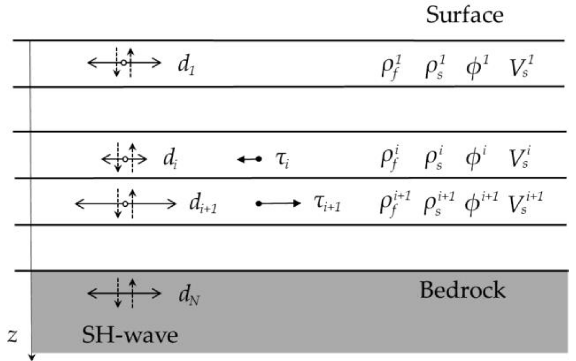
2.1. Improving the NERA Algorithm To Incorporate Biot and Gassman Models

Description of wave propagation in porous fluid-saturated soil began with the studies by J. Frenkel [29] and M.A. Biot [26,27]. Biot’s linear theory of poroelastic wave propagation is valid under the assumptions about a bound and isotropic porous medium, the pore-scale much smaller in comparison with the wavelength and small deformations that ensure linear elastic material behavior.

Biot’s equations of motion for an isotropic fluid-saturated porous medium are given by [30]:

$$\frac{\partial {\tau }_{ij}}{\partial x_j}=\rho {\ddot{d}}_i+{\rho }_f{\ddot{w}}_i$$

(1)

$$\frac{\partial p_f}{\partial x_i}+{\rho }_f{\ddot{d}}_i=-Y{\dot{w}}_i$$

(2)

$$w_i=\varphi \left(d^f-d_i\right)$$

(3)

$$Y=\frac{\eta }{k\left(\omega \right)}$$

(4)

where d is the displacement of the soil matrix, d^f is the displacement of the fluid particles, w is the displacement of the fluid particles relative to the matrix, ρ is the total density of the porous medium, ρ_f is the density of the fluid, p_f is the pore pressure, ϕ is the porosity, d^f is the displacement of the liquid phase, Y is the viscodynamic operator, η is the dynamic viscosity coefficient of the pore fluid, k(ω)—dynamic permeability (frequency-dependent), and ${\tau }_{ij}$ are the stress tensor elements. The dot denotes the time derivative.

To relate the elastic parameters of a porous medium, Gassmann’s equations are commonly used [28]. Gassmann’s theory is based on the assumption that the relative motion of fluid and matrix has a negligible effect on the seismic waves propagation in fluid-saturated soils. Gassmann’s equations are essentially the lower frequency limit of Biot’s more general equations of motion for poroelastic materials. The boundary of the low-frequency range is defined as follows [31]:

$$f<0.1\frac{\eta \varphi }{2\pi k{\rho }_f}$$

(5)

where k is the permeability of the rock.

In this frequency range, Biot’s theory is in accordance with the conclusions from Gassmann’s theory. In different studies, the value of the cutoff frequency varies. According to [32], the cutoff frequency is within the range of 1–20 kHz. In [33], it is argued that Gassmann’s equations give the most accurate results at frequencies lower than 100 Hz. It follows from this that Gassmann’s theory is well applicable to seismology.

According to Gassman’s theory, since the fluid and solid matrix particles move together, the density of the porous medium can be averaged as follows:

$$\rho =\varphi {\rho }_f+\left(1-\varphi \right){\rho }_s$$

(6)

where ρ_s is the density of the solid grains.

Thus, for modeling seismic waves propagation through porous water-saturated soil layers within a seismology frequency band (lower than 100 Hz), the main assumptions for the elementary volume of porous soil are as follows: first, at low frequencies during the passage of the wave, the pore pressure gradients have time to compensate; second, there is no relative motion of the fluid and rock matrix, and, third, there is no movement of the pore fluid beyond the elementary soil volume. Squeezing out fluid from an elementary volume entails an increase in pore pressure in neighboring elements. This process can have an avalanche nature and, under certain conditions, lead to a liquefaction effect. Liquefaction is not considered in the present study.

Taking into account the above assumptions, Biot’s equations of motion for SH-wave for each node in a one-dimensional layered soil deposit system take the form (Figure 1):

$$\left(\varphi {\rho }_f+\left(1-\varphi \right){\rho }_s\right)\frac{{\partial }^{2}d}{\partial t^2}=\frac{\partial \tau }{\partial z}$$

(7)

$$\frac{\partial p_f}{\partial x}=-{\rho }_f\frac{{\partial }^{2}d}{\partial t^2}$$

(8)

IM-model implemented in the NERA code is based on simulating nonlinear hysteretic stress–strain curves using a series of mechanical elements that have different stiffness and sliding resistance. Furthermore, IM-model assumes the Masing rule [34] implementation. The central difference method is used for solving a governing equation of motion.

Assuming the Kelvin–Voigt viscoelastic model, the governing equation of motion for the NERA algorithm [6] (Equation (25)) can be rewritten as follows:

$$\left(\varphi {\rho }_f+\left(1-\varphi \right){\rho }_s\right)\frac{{\partial }^{2}d}{\partial t^2}+\mu \frac{\partial d}{\partial t}=\frac{\partial \tau }{\partial z}$$

(9)

where μ is a mass-proportional damping coefficient.

The spatial and time discretization of the equation of motion, as well as the boundary conditions on the surface and on the basement of the soil deposit system, described in [6], are unchanged. It should be emphasized that pore water motion does not have a shear component [19], so shear stresses emerging during SH-waves propagation and explicitly present in the equation of motion (9) are not affected by pore water or water column above the offshore site.

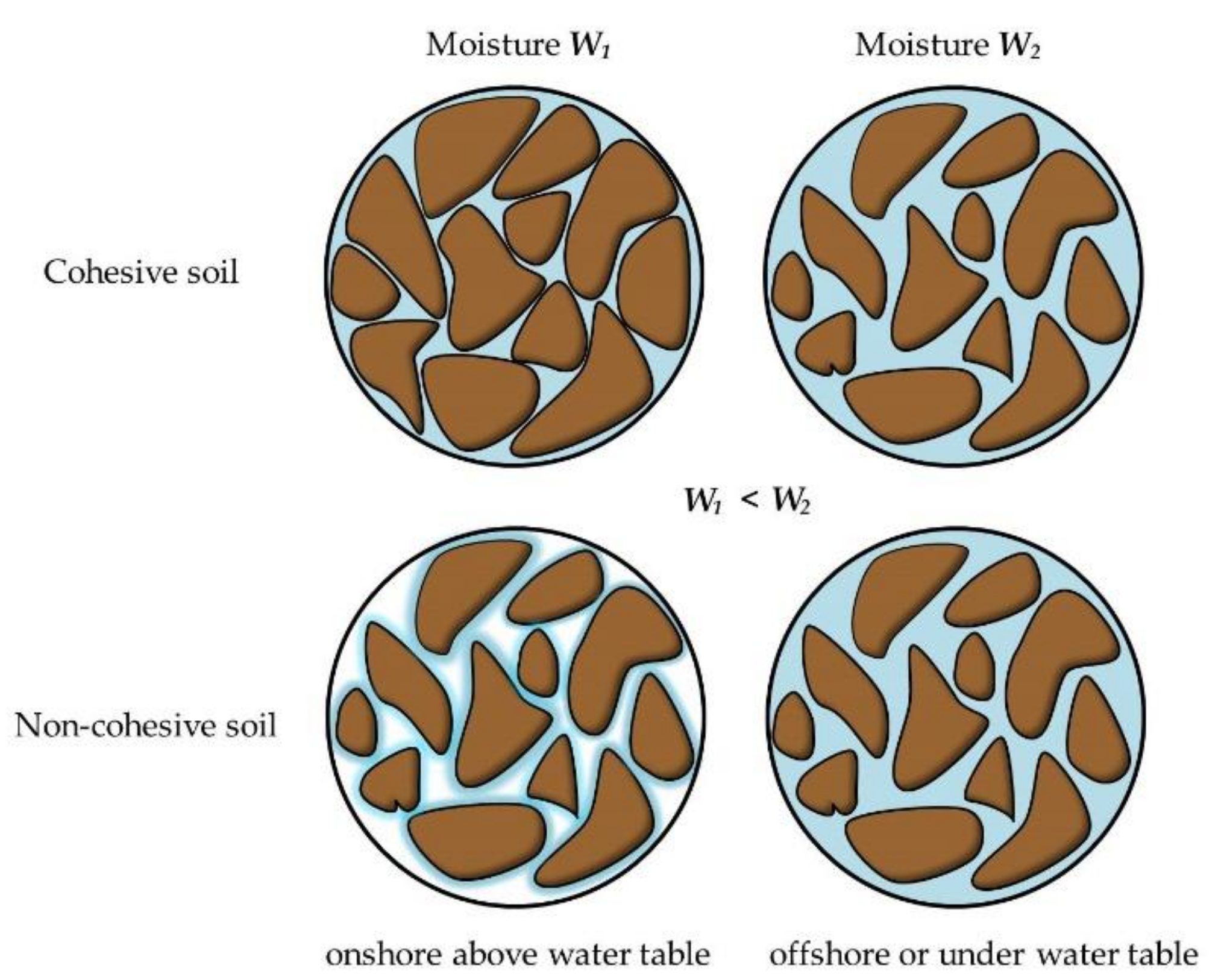
2.2. The Models of Elementary Volume of Cohesive/Non-Cohesive Soils

According to their structure, composition and physical properties, soils are divided into two general groups: dense and loose. Loose soils are of particular interest from a geotechnical point of view, including sandy and clayey soils. In this study, the sandy soils were considered non-cohesive and clayey soils—as cohesive.

Non-cohesive sandy soils with a solid matrix are characterized by a negligible change in porosity, while fluid saturation of the porous space can vary significantly. The fluid saturation coefficient, to a certain extent, affects the properties of the sandy soils as the basement for structures. Non-cohesive onshore soils in situ usually have a notable fraction of pore fluid even when located above the water table, whereas the amount of pore space without fluid (with air) can be presumed as negligible at offshore sites or below the water table at onshore sites.

In favor of the above statements is the fact that in single-grained soils like sand, water percolates quickly through the soil, while in massive soils, such as clays, water movement is relatively slow. This is also due to the pore size, as capillary suction increases as pore size decreases, which is why water is held more tightly in micropores present in clay-dominated soils [35]. This leads to the fact that the clayey soils are often expansive, i.e., natural clay deposits exhibit significant volume changes due to water content variation, while remaining perpetually saturated (i.e., degree of saturation is one). This process is governed by the attraction of bipolar water molecules to the negatively charged clay particles [36,37]. In turn, the combination of adsorptive and capillary forces in both cohesive and non-cohesive soil makes it hard to gain zero moisture in natural conditions [35].

Therefore, it is supposed that elementary volume of non-cohesive soil: first, has constant porosity; second, is a three-phase (air–fluid–solid) medium at onshore sites above the water table and two-phase (fluid–solid) medium at either offshore sites or below the water table at onshore sites (Figure 2).

For cohesive clayey soils, as their fluid saturation coefficient is close to unity, the total water content and the degree of cohesion caused by it are more significant. The amount of water contained in cohesive soils depends primarily on the volume of the pore space. Thus, it is supposed that elementary volume of cohesive soils: first, has variable porosity; second, is a two-phase (fluid–solid) medium both at onshore and offshore sites (Figure 2).

The Equation (6) for averaging the density of porous saturated soils is suitable for cohesive soils when the whole pore space is always filled by the fluid. For non-cohesive soils, it is more suitable to use the following equation for averaging the density:

$$\rho ={\rho }_m\left(1+W\right)$$

(10)

where ρ_m is a density of the solid matrix and W is a moisture coefficient defined as follows:

$$W=\frac{S_{r}e{\rho }_f}{{\rho }_S}\left\{\begin{array}{c}e\ne const,S_r=1=const,forcohesivesoils\\ e=const,S_r\ne const,fornon-cohesivesoils\end{array}\right.$$

(11)

where e is a void ratio, S_r is a saturation factor (saturated pore volume fraction).

The governing equation of motion (9) can be rewritten as follows:

$$\left\{\begin{array}{c}\left(\varphi {\rho }_f+\left(1-\varphi \right){\rho }_s\right)\frac{{\partial }^{2}d}{\partial t^2}+\mu \frac{\partial d}{\partial t}=\frac{\partial \tau }{\partial z}forcohesivesoils\\ {\rho }_m\left(1+W\right)\frac{{\partial }^{2}d}{\partial t^2}+\mu \frac{\partial d}{\partial t}=\frac{\partial \tau }{\partial z}fornon-cohesivesoils\end{array}\right.$$

(12)

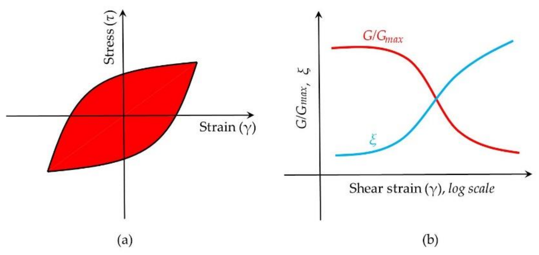
2.3. Maximum Shear Modulus G_max and Shear Modulus Degradation Curves G/G_max

The typical description of nonlinear soil behavior are models that rely on hysteresis stress–strain relations. With NERA, the hysteresis curve is modeled using such parameters as maximum shear modulus G_max and so-called shear modulus degradation curves G/G_max (γ) (Figure 3).

The easiest way to obtain G_max for each sublayer of the soil deposit is to use known values of the averaged density ρ of saturated porous medium and shear wave velocity Vs derived from the geophysical and geotechnical investigations:

$$G_{max}=\rho V_s^2$$

(13)

However, there are some empirical expressions derived from laboratory tests that demonstrate the dependency of G_max on different parameters, including a void ratio. The following example is for seabed clayey soils [38]:

$$G_{max}=\frac{358-3.8PI}{0.4+0.7e}\left({\sigma }_0^{\prime }\right)$$

(14)

In turn, the following example is for sandy soils with round particles [19]:

$$G_{max}=700\frac{{\left(2.17-e\right)}^2}{1+e}{\left({\sigma }_0^{\prime }\right)}^{0.5}$$

(15)

where PI is a plasticity index, σ₀′ is the average effective mean stress level, which can be expressed as [39]:

$${\sigma }_0^{\prime }=\frac{\left(1+2K_0\right)}{3}{\sigma }_v^{\prime }{K}_0=0.0042PI+0.44$$

(16)

where σ_v′ is effective vertical stress.

Many data on nonlinear dynamic deformation features of soils were obtained from drained tests, while the effects of drainage are not negligible in the real ground [19]. In this regard, the following expression was obtained for undisturbed undrained samples [40]:

$$\frac{G}{G_{max}}=\left(A_1+A_{2}lg{D}_{50}\right){\sigma }_0^{\prime }{}^{\left(B_1+B_{2}lg{D}_{50}\right)}$$

(17)

where D₅₀ is a mean particle size of sand (mm) and A₁, A₂, B₁, B₂ are strain-dependent empirical parameters.

For cohesive soils, the following empirical expression is more suitable that includes a plasticity index PI [41]:

$$\frac{G}{G_{max}}=K\left(\gamma ,PI\right){\left({\sigma }_0^{\prime }\right)}^{m\left(\gamma ,PI\right)-m_0}$$

(18)

where K(γ, PI) and m(γ, PI) are functions that depend on strain γ and plasticity index PI.

One can conclude that maximum shear modulus G_max depends on a void ratio either implicitly (Equation (13) or explicitly (Equations (14) and (15)). Meanwhile, shear modulus degradation curves G/G_max (γ) under undrained conditions considerably depend on the mean effective stress, as well as the plasticity index or mean size of soil particles (Equations (17) and (18)), but not on a void ratio. Special comparative analyses also showed conflicting results on the influence of the void ratio on the form of the shear modulus degradation curves of cohesive soils [42]. Hence, it is assumed here that shear modulus degradation curves do not require special modifications to consider a porous medium. The same is true to the damping ratio curves, as additional damping is not considered due to the lack of relative motion of the soil matrix and pore fluids. Therefore, in this study, the classic relationships from the literature were used.

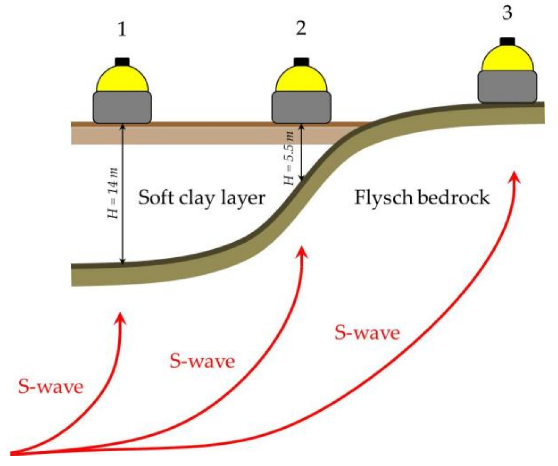
2.4. Modeling the Response of Soft Clay Layer at the Black Sea Offshore Site

The algorithm described above was used for modeling the response of a soft clay layer at the Black Sea offshore site. The input data were derived from the results of geotechnical engineering and seismological studies conducted in the northeast shelf zone of the Black Sea near the Anapa city in 2011 for seabed pipeline projecting.

We used seismic records of the 2011 Kütahya earthquake, which occurred on 2011–05–19 20:15:25.09 UTC and had magnitude M_s = 5.8 [43]. The seismic signals of this event were recorded by three ocean-bottom seismometers (OBS) temporarily deployed on the Black Sea shelf for local microseismicity monitoring. One OBS was located on the hard flysch outcrop (V_s = 1200 m/s, ρ = 2.6 g/cm³), while other OBS was located on the surface of the soft clay layer of 5.5 m and 14 m thickness, respectively underlain by the flysch bedrock (Figure 4). The main parameters of the soil layers and flysch bedrock, such as thicknesses, velocities and porous medium parameters, were derived from the results of seismic surveys and core sampling. Geotechnical parameters of the clay are presented in

Table 1. Geotechnical parameters of the soft clay at the sites on the shelf near the Anapa city.

Moisture Coefficient, W	Plasticity Index, PI	Density of Solid Grains, ρS (g/cm3)	Density of Solid Matrix, ρm (g/cm3)	Mean Density, ρ (g/cm3)	Void Ratio, e	Saturation Factor, Sr	S-wave Velocity, Vs (m/s)
0.75	21.4	2.71	0.88	1.54	2.08	1	80

.

The Kütahya earthquake S-waves records of these OBS were chosen for modeling because the epicentral distance of this event (920 km) highly exceeds the maximum spacing between OBS (14 km). In this case, the effect of intermediate wave paths differs negligibly, and the records obtained on the flysch outcrop can be used as input motions at the flysch bedrock covered by the soft clay layer. The records acquired on the surface of the clay layer were used for comparison with modeling results. Figure 5 shows the time histories of the S-waves derived from the OBS records and used as input signals at bedrock and verification signals on the surface of the layers.

2.5. Modeling of the Response of Synthetic Soil Deposits With Porous Medium Parameters Specific for Low Moisture Onshore and High Moisture Offshore Sites

This section is dedicated to numerical simulation and comparison of the responses of porous water-saturated layers of cohesive and non-cohesive soils with parameters specific for low moisture onshore and high moisture offshore sites. For this purpose, synthetic soil layers were constructed (Figure 6) using some values of thickness and geotechnical parameters derived from different marine engineering studies. The parameters of the offshore soils presented in

Table 2. Input parameters for the case of sandy layer underlain by the flysch half-space.

Moisture Coefficient, W	Density of Solid Grains, ρS (g/cm3)	Density of Solid Matrix, ρm (g/cm3)	Density of Pore Water, ρf (g/cm3)	Mean Density, ρ (g/cm3)	Void Ratio, e	Saturation Factor, Sr	S-Wave Velocity, Vs (m/s)
0.29 offshore 0.09 onshore	2.75	1.52	1	1.96 offshore 1.66 onshore	0.81	1 offshore 0.3 onshore	280 offshore 305 onshore

,

Table 3. Input parameters for the case of clayey silt layer underlain by the flysch half-space.

Moisture coefficient, W	Density of Solid Grains, ρS (g/cm3)	Density of Solid Matrix, ρm (g/cm3)	Density of Pore Water, ρf (g/cm3)	Mean Density, ρ (g/cm3)	Void Ratio, e	Saturation Factor, Sr	S-wave Velocity, Vs (m/s)
0.70 offshore 0.25 onshore	2.68	1.01	1	1.59 offshore 2.01 onshore	1.85 offshore 0.67 onshore	1 offshore 1 onshore	150 offshore 186 onshore

,

Table 4. Input parameters for the case of soft clay layer underlain by the flysch half-space.

Moisture Coefficient, W	Density of Solid Grains, ρS (g/cm3)	Density of Solid Matrix, ρm (g/cm3)	Density of Pore Water, ρf (g/cm3)	Mean Density, ρ (g/cm3)	Void Ratio, e	Saturation Factor, Sr	S-wave Velocity, Vs (m/s)
0.75 offshore 0.25 onshore	2.71	0.88	1	1.54 offshore 2.02 onshore	2.08 offshore 0.68 onshore	1 offshore 1 onshore	80 offshore 102 onshore

were derived from the results of seismic surveys and core sampling, while the values for their onshore analogs were calculated using Equations (6), (10), (11), (13)–(15) with assumed moisture W and saturation factor Sr. Here it is assumed that clay and clayey silt are cohesive soil and sand is non-cohesive soil. Flysch half-space (V_s = 1200 m/s, ρ = 2.6 g/cm³) is used as underlain bedrock for all synthetic profiles.

For each soil profile, calculations were carried out using three sets of artificial input accelerograms with different peak ground acceleration (PGA) synthesized by the method proposed in [44]. Each set consists of five signals to reduce the stochastic scatter of modeling results by averaging obtained response spectra. Three sets of the main parameters of the simulated earthquake are as follows: M_s = 4.5, R_epi = 20 km; M_s = 6.0, R_epi = 10 km; M_s = 7.0, R_epi = 10 km.

Figure 7 shows the shear moduli degradation curves and damping ratio curves used in this study. The curves used in this study were presented by Schnabel et al. (1973) [45] for flysch half-space, by Sun et al. (1988) [42] for cohesive soils and by Seed and Idriss (1970) [46] for non-cohesive soil.

3. Modeling Results and Discussion

3.1. The Response of Soft Clay Layer at the Black Sea Offshore Site

There is much less OBS data worldwide than obtained at onshore sites. These are mostly collected in the framework of temporary observations with the local networks or arrays, except a few long-term cabled systems. In addition, detailed geotechnical information, including velocity profiles and porous medium parameters of the soils, are usually unknown for OBS networks. Especially it concerns downhole array data at offshore sites. Onshore downhole array data are commonly used to validate earthquake response simulation techniques. However, the offshore data are usually not freely available and mostly comes from vertical seismic profiling, which is an expensive engineering survey.

In the present study, we used seismic signals of the 2011 Kütahya earthquake obtained by three OBS located on the Black Sea shelf. The main purpose of this temporary local network monitoring was local microseismic events acquisition, so the Kütahya earthquake was the only one to make it possible to neglect the effects of intermediate wave paths.

The assumption of no relative movement between fluid and solid at low frequencies leads to using the mean density of the porous soils calculated with Equations (6) and (10) in time-domain equations of motion. The maximum shear modulus G_max and, as a consequence (Equation (13)), V_s also depends on the void ratio. Hence, mean density and shear wave velocity are only parameters, which explicitly depend on the porous structure of the soil. Here, the porous parameters were built-in equations of motion of the NERA code explicitly (see Equation (12)). However, the same reasoning, described in Section 2.1, Section 2.2 and Section 2.3, can be applied for other codes, either equivalent-linear or nonlinear. Hence, the calculated mean densities and shear wave velocities were used as input parameters also for DEEPSOIL code running in equivalent-linear (EQL) and time-domain nonlinear cases (MKZ).

In Figure 8a, the response spectra of the horizontal component of the S-wave are presented both from modeled and experimental records (OBS site with soft clay layer of 5.5 m thickness). The synthetic and observed spectra are largely consistent with each other. The curves for NERA and EQL cases are very similar and slightly overestimated, while the response obtained by the MKZ model is underestimated. Nevertheless, the position of resonant frequency obtained by the MKZ model is more precise. The similarity of the curves for NERA and EQL cases can be due to small strains and near-linear stress–strain dependency while loading (Figure 8b). At the same time, two different constitutive models for nonlinear cases (IM-model for NERA and MKZ-model for DEEPSOIL) gave a more pronounced difference.

There is a clear spectral spike corresponding to a frequency of 3–4 Hz for both synthetic and observed records. The existence of this spike is explained by resonance due to the presence of a layer with rather contrasting S-wave impedance. The impedance of the flysch is 3120 [m*g/s/cm³], while the impedance of the soft clay is 123 [m*g/s/cm³]. The observed resonant frequency corresponds to the value 3.6 Hz, calculated by the well-known empirical equation [47]:

$$f=\frac{V_S}{4H}$$

(19)

where H = a thickness of the layer.

A slight shift between simulated and observed spectra may be due to uncertainty in determining the thickness of the soft clay layer under the seismograph because the dominant frequency in response spectra depends on the layer thickness [48,49].

Figure 9 shows results at the OBS site with a soft clay layer of 14 m thickness, which is similar to those shown in Figure 8. The synthetic and experimental responses are also largely consistent with each other. The main observed resonant frequency also corresponds to the value 1.4 Hz, calculated by the Equation (19).

In Figure 9, it can be seen that resonant spikes are more pronounced in the modeled spectra rather than experimental ones. This may be due to the excessive contrast boundary between the flysch bedrock and the soft clay layer in the synthetic soil profile. In real settings, some impedance gradients might be observed. In this case, the simulated response spectrum would be smoother, as is the case with the spectra of the observed signals.

In addition, it is necessary to take into account the nonlinear behavior of the soil, including such effects as S-wave signal saturation when ground motion amplitudes stop increasing with an increase of macroseismic intensity and damages [50,51]. At high values of macroseismic intensity, loose soils begin to collapse by seismic waves, plastic behavior and soil flow, cracks, etc., appear. On one hand, collapsing soils lose their bearing capacity: they can no longer serve as a basement for buildings and structures. On the other hand, a high-amplitude wave cannot propagate through weak soil. The weaker the soil (the lower its impedance), the lower the maximum wave amplitude that can be observed on its surface [51]. It is mainly about accelerations but not displacements (see below).

The spectra in Figure 9 (for 14 m thickness) lie lower than the spectra in Figure 8 (for 5.5 m thickness). It could be due to the attenuation of the S-waves and also due to the described mechanism causing S-wave amplitudes saturation. This behavior is seen in both observed and synthetic spectra.

In Figure 10, the approximating curves are shown for the simulated peak ground accelerations (PGA), peak ground velocities (PGV) and peak ground displacements (PGD) on the surface of a soft clay layer with different thickness (3 m, 10 m and 14 m), while different input accelerograms on the bedrock are applied. The amplitude saturation effect is clearly seen. First, the larger thickness of the soft clay layer, the faster saturation occurs. In turn, for calculating macroseismic intensity increase, the mean impedance is used calculated for the soil thickness of 10 or 30 m [24]. Thus, the larger thickness of the soft clay layer, the lower the mean impedance of the upper 10 or 30 m of the soil profile. Second, the saturation effect is less distinguished for velocities than for accelerations, while the displacements, in this case, are in accordance with macroseismic intensity and level of damages.

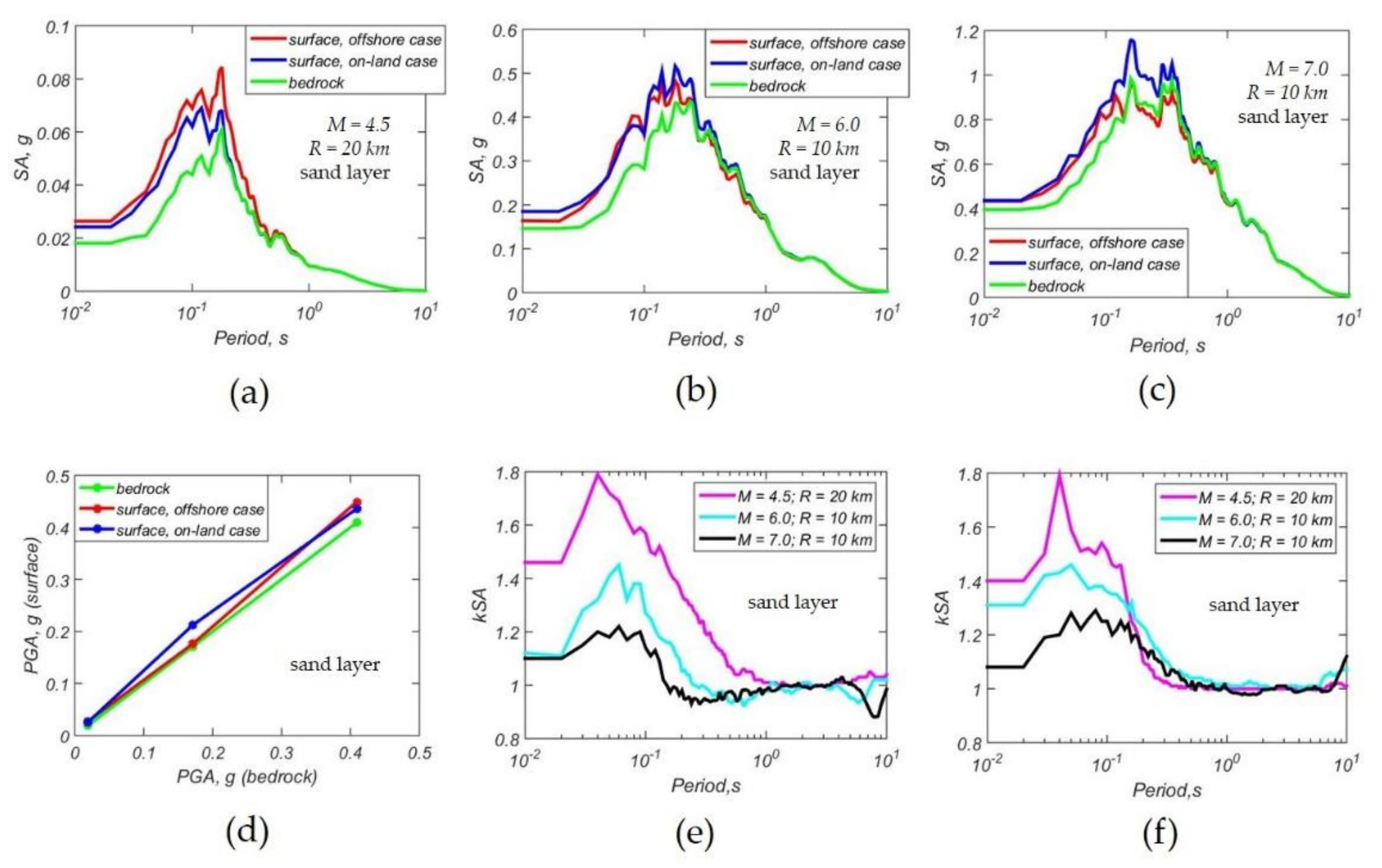
3.2. The Response of Synthetic Soil Deposits With Porous Medium Parameters Specific for Low Moisture Onshore and High Moisture Offshore Sites

In Figure 11, Figure 12, Figure 13, the results are shown for input modeling data described in Section 2.5. In each case, the spectra of the seismic signal at the bedrock are compared with the surface spectra for low moisture onshore and high moisture offshore sites. Corresponding surface and bottom PGA values and acceleration amplification curves are also presented.

In Figure 11a–c, it is seen that for clayey silt, the clear resonance is observed due to interactions of the predominant period of input motion and natural site period. At the same time, Figure 11d shows that the PGA curve for offshore cases starts to flatten in contrast to the PGA curve for onshore cases. It can be due to the smaller value of the S-wave impedance for soft clay for the offshore case. Therefore, acceleration amplitudes for offshore cases saturate faster. Figure 11e–f shows that the acceleration amplification values generally decrease with an increase of seismic load at bedrock, while resonant periods shift to the long-period range. A decrease in amplification and shift in resonant periods are more pronounced for the offshore case.

In the case of soft clay (Figure 12), the situation is almost the same. However, the effect of amplitude saturation occurs faster. Soft clay is such a weak soil that even with a relatively small seismic load at bedrock, the amplitude of surface accelerations for W = 0.7 is already in a state of saturation—it is slightly lower than the amplitude of surface accelerations for W = 0.25.

In Figure 13a–c, e–f it is seen that the spectra for sand for onshore and offshore cases differ insignificantly. There are no clear resonances. It can be due to the very low value of the natural site period for the layer thickness of 2.2 m (T = 0.03 s or f = 33 Hz), which is close to the Nyquist frequency (sampling rate is 100 Hz) and corresponding slope of the spectra curve. However, Figure 13d shows that acceleration amplitudes for the onshore case saturate faster because the S-wave impedance for the onshore case is lower.

The difference in the behavior of the spectra for sandy and clayey soils can be explained by the fact that for clayey silt and soft clay soils, there is a significant drop of the S-wave impedance of the soil with increasing moisture. The boundary between flysch and clayey silt or soft clay becomes more contrasting, and resonance is observed.

Thus, the response of cohesive and non-cohesive soils with moisture specific both for onshore and offshore sites is explained by effects of resonances and the effect of seismic amplitude saturation, which, in turn, depend on the corresponding value of the layer thickness and S-wave impedance for porous saturated soil layer.

4. Conclusions

Summarizing all the above, it is possible to come to the following conclusions:

(1) The presented procedure allows developing the NERA algorithm to incorporate the case of porous saturated soils, including those located offshore. The Biot and Gassman models in the seismological low-frequency band are reduced to using the parameters of porous medium for averaging the density of porous soils and calculating the velocity of S-waves in governing equation of the NERA algorithm. In turn, shear modulus degradation curves for undrained undisturbed settings do not depend significantly on the parameters of the porous medium. The water layer above the offshore site also does not affect the response in the case of SH-waves;

(2) The use of the presented procedure for modeling the response of offshore soft clay layer showed good agreement between the simulated by different methods (NERA, DEEPSOIL (EQL) and DEEPSOIL (MKZ)) and observed spectra on the layer surface. The algorithm allows demonstrating resonances and the effect of the seismic wave amplitude saturation;

(3) The modeling showed that the response of cohesive and non-cohesive soils with moisture specific both for onshore and offshore sites is explained by effects of resonances and effect of seismic amplitude saturation, which, in turn, depend on the corresponding value of the layer thickness and S-wave impedance for porous saturated soil layer;

(4) The presented procedure and modeling results can have significant practical usage for studying the influence of parameters of the porous medium on the seismic response of the moist soil deposits. Offshore geophysical and geotechnical studies are quite expensive, especially if a large measurement grid is required. The proposed approach makes it possible to use the analogy method in offshore site response analysis, taking as a basis the main geotechnical parameters of the corresponding coastal soils and adjusting the values of void ratio, water saturation factor and moisture coefficient. In addition, it is also possible to interpolate the values of the parameters of a saturated porous medium on a sparse grid at the offshore area of interest.

References

1. Kramer, S.L.; Paulsen, S.B. Practical Use of Geotechnical Site Response Models. In Proceedings of the International Workshop on Uncertainties in Nonlinear Soil Properties and Their Impact on Modeling Dynamic Soil Response, Berkeley, CA, USA, 18–19 March 2004; p. 10. [Google Scholar]
2. Stewart, J.P.; Afshari, K.; Hashash, Y.M.A. Guidelines for Performing Hazard-Consistent One-Dimensional Ground Response Analysis for Ground Motion Prediction; Pacific Earthquake Engineering Research Center, University of California: Berkeley, CA, USA, 2014; 139p. [Google Scholar]
3. Schnabel, P.B.; Lysmer, J.; Seed, H.B. SHAKE: A Computer Program for Earthquake Response Analysis of Horizontally Layered Sites; Earthquake Engineering Research Center, University of California: Berkeley, CA, USA, 1972; 102p. [Google Scholar]
4. Bardet, J.P.; Ichii, K.; Lin, C.H. EERA: A Computer Program for Equivalent Linear Earthquake Site Response Analysis of Layered Soils Deposits; University of Southern California: Los Angeles, CA, USA, 2000; 38p. [Google Scholar]
5. Kottke, A.R.; Rathje, E.M. Technical Manual for Strata; PEER Report 2008/10; Pacifc Earthquake Engineering Research Center: Berkeley, CA, USA, 2008; 100p. [Google Scholar]
6. Bardet, J.P.; Tobita, T. NERA: A Computer Program for Nonlinear Earthquake Site Response Analyses of Layered Soil Deposits; University of Southern California: Los Angeles, CA, USA, 2001; 44p. [Google Scholar]
7. Iwan, W.D. On a class of models for the yielding behavior of continuous and composite systems. J. Appl. Mech. 1967, 34, 612–617. [Google Scholar] [CrossRef]
8. Mróz, Z. On the description of anisotropic workhardening. J. Mech. Phys. Solids 1967, 15, 163–175. [Google Scholar] [CrossRef]
9. Hashash, Y.M.A.; Musgrove, M.I.; Harmon, J.A.; Ilhan, O.; Xing, G.; Numanoglu, O.; Groholski, D.R.; Phillips, C.A.; Park, D. DEEPSOIL 7, User Manual; Board of Trustees of University of Illinois at Urbana-Champaign: Urbana, IL, USA, 2020; 170p. [Google Scholar]
10. Matasovic, N. Seismic Response of Composite Horizontally-Layered Soil Deposits. Ph.D. Thesis, University of California, Los Angeles, CA, USA, 1993. [Google Scholar]
11. Kramer, S.L. Geotechnical Earthquake Engineering; Prentice Hall: Upper Saddle River, NJ, USA, 1996; 653p. [Google Scholar]
12. Hao, H. Effects of Spatial Variation of Ground Motions on Large Multiply Supported Structures; UCB/EERC-89-06; University of California: Berkeley, CA, USA, 1989; 168p. [Google Scholar]
13. Li, C.; Hao, H.; Li, H.; Bi, K.; Chen, B. Modeling and Simulation of Spatially Correlated Ground Motions at Multiple Onshore and Offshore sites. J. Earthq. Eng. 2017, 21. [Google Scholar] [CrossRef]
14. Prevost, J.H. DYNAFLOW™ Version 02 Release 10.A. 2010. 516p. Available online: https://blogs.princeton.edu/prevost/wp-content/uploads/sites/192/2013/11/dynaflow-v02.10.A-full-manual-2010.pdf (accessed on 22 December 2020).
15. PLAXIS 3D Reference Manual. 2016. Available online: https://communities.bentley.com/products/geotech-analysis/w/plaxis-soilvision-wiki/46137/manuals---plaxis (accessed on 22 December 2020).
16. ITASCA Consulting Group, Inc. FLAC3D—Fast Lagrangian Analysis of Continua in Three-Dimensions, Ver. 6.0. 2017. Available online: https://www.itascacg.com/software/downloads/flac3d-downloads (accessed on 22 December 2020).
17. Ye, J. Seismic response of poro-elastic seabed and composite breakwater under strong earthquake loading. Bull. Earthq. Eng. 2012, 10, 1609–1633. [Google Scholar] [CrossRef]
18. Diao, H.; Hu, J.; Xie, L. Effect of seawater on incident plane P and SV waves at ocean bottom and engineering characteristics of offshore ground motion records off the coast of southern California, USA. Earthq. Eng. Eng. Vib. 2014, 13, 181–194. [Google Scholar] [CrossRef]
19. Towhata, I. Geotechnical Earthquake Engineering; Springer: Berlin/Heidelberg, Germany, 2008; p. 684. [Google Scholar] [CrossRef]
20. Stewart, J.P.; Boore, D.M.; Seyhan, E.; Atkinson, G.M. NGA-West2 equations for predicting vertical-component PGA, PGV, and 5%-damped PSA from shallow crustal earthquakes. Earthq. Spectra 2016, 32, 1005–1031. [Google Scholar] [CrossRef]
21. Tsai, C.-C.; Liu, H.-W. Site response analysis of vertical ground motion in consideration of soil nonlinearity. Soil Dyn. Earthq. Eng. 2017, 102, 124–136. [Google Scholar] [CrossRef]
22. Beresnev, I.A.; Nightingale, A.M.; Silva, W.J. Properties of Vertical Ground Motions. Bull. Seismol. Soc. Am. 2002, 92, 3152–3164. [Google Scholar] [CrossRef]
23. Boore, D.M.; Smith, C.E. Analysis of earthquake recordings obtained from the seafloor earthquake measurement system (SEMS) instruments deployed off the coast of Southern California. Bull. Seismol. Soc. Am. 1999, 89, 260–274. [Google Scholar]
24. Medvedev, S.V. Engineering Seismology; Gosstrojizdat: Moscow, Russia, 1962; 284p. (In Russian) [Google Scholar]
25. Goto, H.; Tanaka, N.; Sawada, S.; Inatani, H. S-wave impedance measurements of the uppermost material in surface ground layers: Vertical load excitation on a circular disk. Soils Found. 2015, 55, 1282–1292. [Google Scholar] [CrossRef] [Green Version]
26. Biot, M.A. Theory of Propagation of Elastic Waves in a Fluid-saturated Porous Solid I. Low-frequency range. J. Acoust. Soc. Am. 1956, 28, 168–178. [Google Scholar] [CrossRef]
27. Biot, M.A. Theory of Propagation of Elastic Waves in a Fluid-saturated Porous Solid II. Higher frequency range. J. Acoust. Soc. Am. 1956, 28, 179–191. [Google Scholar] [CrossRef]
28. Gassmann, F. Über die Elastizität Poröser Medien; Instut für Geophysik an der ETH: Zurich, Switzerland, 1951. [Google Scholar]
29. Frenkel, J. On the Theory of Seismic and Seismoelectric Phenomena in a Moist Soil. J. Phys. 1944, 111, 230–241, republished in J. Eng. Mech. 2005, 131, 879–887. [Google Scholar] [CrossRef] [Green Version]
30. Wenzlau, F. Poroelastic Modelling of Wavefields in Heterogeneous Media. Ph.D. Thesis, University of Karlsruhe, Kahrsruhe, Germany, 2009; 159p. [Google Scholar]
31. White, J.E. Underground Sound: Application of Seismic Waves. In Seismic Wave Propagation: Collected Works of J. E. White; Society of Exploration Geophysicists: Tulsa, OK, USA, 1983. [Google Scholar]
32. Avseth, P.; Mukerji, T.; Mavko, G. Quantitative Seismic Interpretation: Applying Rock Physics Tools to Reduce Interpretation Risk; Cambridge University Press: Cambridge, UK, 2005; 359p. [Google Scholar] [CrossRef]
33. Mavko, G.; Mukerji, T.; Dvorkin, J. The Rock Physics Handbook: Tools for Seismic Analysis of Porous Media; Cambridge University Press: New York, NY, USA, 2009; 511p. [Google Scholar] [CrossRef]
34. Masing, G. Eigenspannungen und Verfertigung beim Messing. In Proceedings of the 2nd International Congress on Applied Mechanics, Zurich, Switzerland, 1926; pp. 332–335. [Google Scholar]
35. Easton, Z.M.; Bock, E. Soil and Soil Water Relationships; Produced by Communications and Marketing, College of Agriculture and Life Sciences, Virginia Tech. 2016. 9p. Available online: https://digitalpubs.ext.vt.edu/vcedigitalpubs/2481933593189246/MobilePagedReplica.action?pm=2&folio=1#pg1 (accessed on 22 December 2020).
36. Fityus, S.; Buzzi, O. The place of expansive clays in the framework of unsaturated soil mechanics. Appl. Clay Sci. 2009, 43, 150–155. [Google Scholar] [CrossRef]
37. Azam, S.; Ito, M.; Chowdhury, R. Engineering Properties of an Expansive Soil. In Proceedings of the 18th International Conference on Soil Mechanics and Geotechnical Engineering, Paris, France, 2–6 September 2013; pp. 199–202. [Google Scholar]
38. Kagawa, T. Moduli and damping factors of soft marine clays. J. Geotech. Eng. 1992, 118, 1360–1375. [Google Scholar] [CrossRef]
39. Massarsch, K.R. Lateral Earth Pressure in Normally Consolidated Clay. In Proceedings of the 7th European Conference on Soil Mechanics and Foundation Engineering, Brighton, UK, 10–13 September 1979; Volume 2, pp. 245–249. [Google Scholar]
40. Yasuda, S.; Yamaguchi, I. Dynamic Soil Properties of Undisturbed Samples. In Proceedings of the 20th Annual Conference of JSSMFE, Nagoya, Japan, 1985; pp. 539–542. [Google Scholar]
41. Ishibashi, I.; Zhang, X. Unified dynamic shear moduli and damping ratios of sand and clay. Soil Found. 1993, 33, 182–191. [Google Scholar] [CrossRef] [Green Version]
42. Sun, J.I.; Golesorkhi, R.; Seed, H.B. Dynamic Moduli and Damping Ratios for Cohesive Soils; Earthquake Engineering Research Center, University of California: Berkeley, CA, USA, 1988; 42p. [Google Scholar]
43. International Seismological Centre. Available online: http://www.isc.ac.uk/iscbulletin/ (accessed on 22 December 2020).
44. Sabetta, F.; Pugliese, A. Estimation of Response Spectra and Simulation of Nonstationary Earthquake Ground Motions. Bull. Seismol. Soc. Am. 1996, 86, 337–352. [Google Scholar]
45. Schnabel, P.B. Effects of local geology and distance from source on earthquake ground motions. Ph.D. Thesis, University of California, Berkeley, CA, USA, 1973. [Google Scholar]
46. Seed, H.B.; Idriss, I.M. Soil Moduli and Damping Factors for Dynamic Response Analysis; Earthquake Engineering Research Center, University of California: Berkeley, CA, USA, 1970; 48p. [Google Scholar]
47. Kanai, K. Relation between the nature of surface layer and the amplitudes of earthquake motions. Bull. Earth. Res. Inst. 1952, 30, 31–37. [Google Scholar]
48. Krylov, A.A.; Ivashchenko, A.I.; Kovachev, S.A. Assessing influence of local ground conditions on the seismic load intensity in the shelf area—The seismic impedance method and nonlinear earthquake response analysis. Eng. Res. 2016, 3, 46–52. (In Russian) [Google Scholar]
49. Kendzera, A.V.; Semenova, Y.V. The influence of resonant and nonlinear features of soils on seismic hazard of construction sites. Geophys. J. 2016, 38, 3–18. (In Russian) [Google Scholar]
50. Irikura, K.; Kudo, K.; Okada, S.; Sasatani, T. (Eds.) The Effects of Surface Geology on Seismic Motion; Balkema: Rotterdam, The Netherlands, 1998; 806p. [Google Scholar]
51. Gusev, A.A. About seismological basement of earthquake-resistant construction. Phys. Solid Earth 2002, 12, 56–70. (In Russian) [Google Scholar]
Figure 1. One-dimensional layered soil deposit system and its spatial discretization.
Applsci 11 01854 g001
Figure 2. Schematic representation of the elementary volume of cohesive and non-cohesive soil with different moisture values.
Applsci 11 01854 g002
Figure 3. Hysteresis curve (a), shear modulus degradation curves G/Gmax (γ), and damping ratio curves ξ(γ) (b) models for cyclic loading.
Applsci 11 01854 g003
Figure 4. Ocean-bottom seismometers (OBS) deployments at the Black Sea shelf sites: 1—on the surface of the soft clay layer of 14 m; 2—on the surface of the soft clay layer of 5.5 m; 3—on the hard flysch outcrop.
Applsci 11 01854 g004
Figure 5. Input signal at bedrock (a) and verification signals on the surface of the soft clay layers with the thickness of 5.5 m (b) and 14 m (c), derived from the OBS records.
Applsci 11 01854 g005
Figure 6. Synthetic profiles of cohesive and non-cohesive soils used for response modeling in onshore and offshore settings (layer thicknesses: 2.2 m for sand, 6.3 m for clayey silt, 5.5 m for soft clay; other soil parameters, see Table 2, Table 3, Table 4).
Applsci 11 01854 g006
Figure 7. Input soil parameters used in the study: (a) shear moduli degradation curves; (b) damping ratio curves.
Applsci 11 01854 g007
Figure 8. Modeling results for the Black Sea shelf site with soft clay layer of 5.5 m thickness: (a) response spectra SA(T, 5%) obtained by different modeling methods and real record; (b) stress–strain curves at the surface of the layer.
Applsci 11 01854 g008
Figure 9. Modeling results for the Black Sea shelf site with soft clay layer of 14 m thickness: (a) response spectra SA(T, 5%) obtained by different modeling methods and real record; (b) stress–strain curves at the surface of the layer.
Applsci 11 01854 g009
Figure 10. Modeled dependences (polynomial approximation) of peak ground acceleration (PGA) (a), peak ground velocities (PGV) (b) and peak ground displacements (PGD) (c) on the surface of the soft clay layer.
Applsci 11 01854 g010
Figure 11. Modeling results for the case of clayey silt layer: (ac) response spectral acceleration SA (T, 5%); (d) PGA values; (e) acceleration amplification curves for offshore case; (f) acceleration amplification curves for the onshore case.
Applsci 11 01854 g011
Figure 12. Modeling results for the case of soft clay layer: (ac) response spectral acceleration SA (T, 5%); (d) PGA values; (e) acceleration amplification curves for offshore case; (f) acceleration amplification curves for the onshore case.
Applsci 11 01854 g012
Figure 13. Modeling results for the case of sand layer: (ac) response spectral acceleration SA (T, 5%); (d) PGA values; (e) acceleration amplification curves for offshore case; (f) acceleration amplification curves for the onshore case.
Applsci 11 01854 g013