
2-D Seismic Response Analysis of a Slope in the Tyrrhenian Area (Italy)


1
CNR—ISPC National Research Council—Institute of Heritage Science, 95124 Catania, Italy
2
Department of Civil Engineering and Architecture, University of Catania, 95125 Catania, Italy
*
Author to whom correspondence should be addressed.
Appl. Sci. 2021, 11(7), 3180; https://0-doi-org.brum.beds.ac.uk/10.3390/app11073180
Submission received: 20 December 2020
/
Revised: 19 March 2021
/
Accepted: 26 March 2021
/
Published: 2 April 2021
(This article belongs to the Special Issue Seismic Geotechnical Hazards Studies)
Abstract
:The Caronia area is located in the Tyrrhenian north-eastern sector of Sicily (Italy). Starting in 2010, attention focused on the study of landslides phenomena that occurred in this area, which caused significant economic damage to buildings and infrastructures and loss of productive activities. The site is characterized by geotechnical, geological and morphological heterogeneity, and for this reason the site is particularly prone to seismic topographic amplification effects. In this paper, the authors carried out numerical studies focused on the topographic seismic effect evaluation concerning the slope affected by the landslide phenomena. For this site, geotechnical characterization was available concerning both in-situ and laboratory tests; boreholes, piezometers, down-hole tests, multichannel analysis of surface waves tests, seismic tomographies and inclinometer measurements were carried out. Furthermore, 1-D and 2-D local seismic response analyses were carried out by using different synthetic seismograms related to the earthquake of Messina and Reggio Calabria on 28 December 1908. The results of the numerical analyses are presented in terms of response seismograms and response spectra at the surface.
1. Introduction
The effects of the topography and geological conditions on seismic waves have been studied by many authors from the second half of the last century. The observation of the most important earthquakes shows that the presence of topographic irregularities can significantly modify the consequences of the seismic input motion; so much so that even the European Code [1] takes into account the modification of the seismic action due to topography through a topographical amplification factor.
Among the most important experiences that must be remembered include the study on the Pacoima Dam in San Fernando Valley, California [2,3], and also the study on the Pacoima Canyon, which confirmed the very important role of topographic amplification on landslide triggering [4]. In the recent past, the 1999 Athens Earthquake caused heavy damage on the eastern bank of the Kifissos River canyon and inspired the study on the topographic aggravation factor [5].
This paper is focused on the study of the local seismic amplification for a slope located in the Tyrrhenian north-eastern part of Sicily (Italy), carried out through 2-D numerical analyses, to determine the topographical contribution on the ground acceleration [6,7,8,9]. As is known, the local seismic response is significantly influenced by stratigraphic heterogeneity and by morphological irregularities. The surface morphology is relevant on the seismic amplification of the site as evidenced by the structural damages detected in correspondence of morphological elements, such as the slopes, the escarpments and the canyons. From the geotechnical point of view, the topographical amplification involves the evaluation of the seismic risk for the historical sites built on reliefs, but also for earthworks and important works as bridges, dams, natural and artificial slopes. The Italian Building Code (NTC 2018) [10] allows for the evaluation of topographic amplification using a simplified method based on the use of the topographic amplification coefficient ST, which varies from a minimum value of 1.0 to a maximum value of 1.4. However, it is important to consider that the values suggested by NTC 2018 [10] are referring to general and not particular configurations and provide numerical values that in some cases may not be completely realistic. This work concerns the determination of topographic amplification factors that could influence the slope response in the case of seismic events. The topographical amplification factors were therefore calculated with 2-D numerical models and the relative values obtained from the analyses were compared with the values provided by the Italian Building Code.
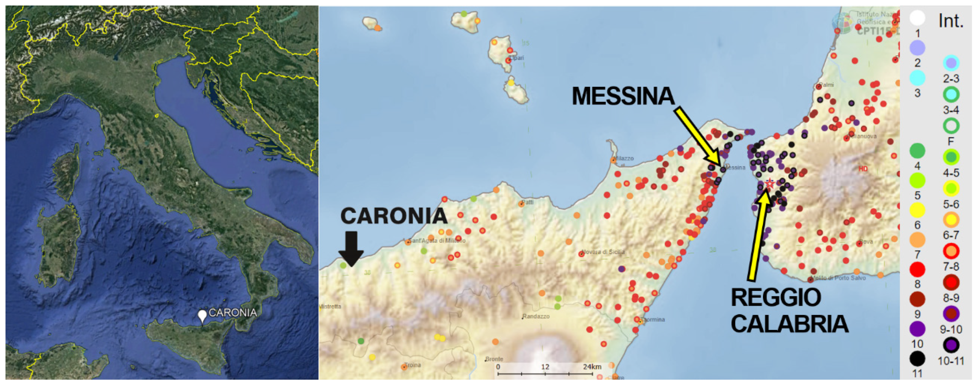
The study area is a portion of the Caronia Municipality (Figure 1), where in 2010 a non-coseismal landslide affected the southern part of the town and caused damages to urbanized areas and infrastructures; in addition, about 120 inhabitants in an area of approximately 50 hectares were evacuated.
2. Site Characterization
2.1. Seismicity of the Study Area
The northern part of Sicily, in front of the Tyrrhenian Sea where Caronia is located, is a place of frequent, intense and deep seismicity [11]. This peculiarity attracted many seismologists, explaining the large number of papers dealing with it [12,13]. The area is prone to high seismic risk, and in the coastal part, to high tsunami risk. The strongest historical earthquake recorded in the area is also the strongest Italian earthquake, which took place in the Messina Strait on 28 December 1908, causing an estimated 60,000 to 120,000 fatalities and the destruction of Messina, Reggio Calabria and many other cities in Calabria and Sicily. The 1908 earthquake, which was felt strongly in Sicily and Calabria (both regions of southern Italy), was caused by normal faulting in the Messina Strait starting at 05:20 a.m. on 28 December and lasting about 30 s. The earthquake was also felt in the middle Italy regions of Campania and Molise, as well as on the Malta Island (south of Sicily).
The shorelines of Messina and Reggio Calabria were stricken by up to 12 m waves, completing the devastation and displacing a large quantity of rubble from collapsed buildings. As a consequence of the disaster, in the areas all communications were disrupted and rescue operations began right from the sea thanks to the presence of English ships first and then also Russian ships to give immediate aide to the populations. The medical officers of the Royal Navy and the Baltic Guard-Marine gave the first medical aid to the victims [14].
Due to poor quality of construction and construction materials, the damage in Messina and Reggio Calabria was very strong and contributed to delivering the coup de grace in the same areas that had already suffered seismic events in the previous 15 years, such as the 1894, 1905 and 1907 southern Calabria earthquakes, all characterized by Me > 6 [15]. Historic records also report that the Ionian Islands off the west coast of Greece and other countries such as Albania and Montenegro felt the earthquake.
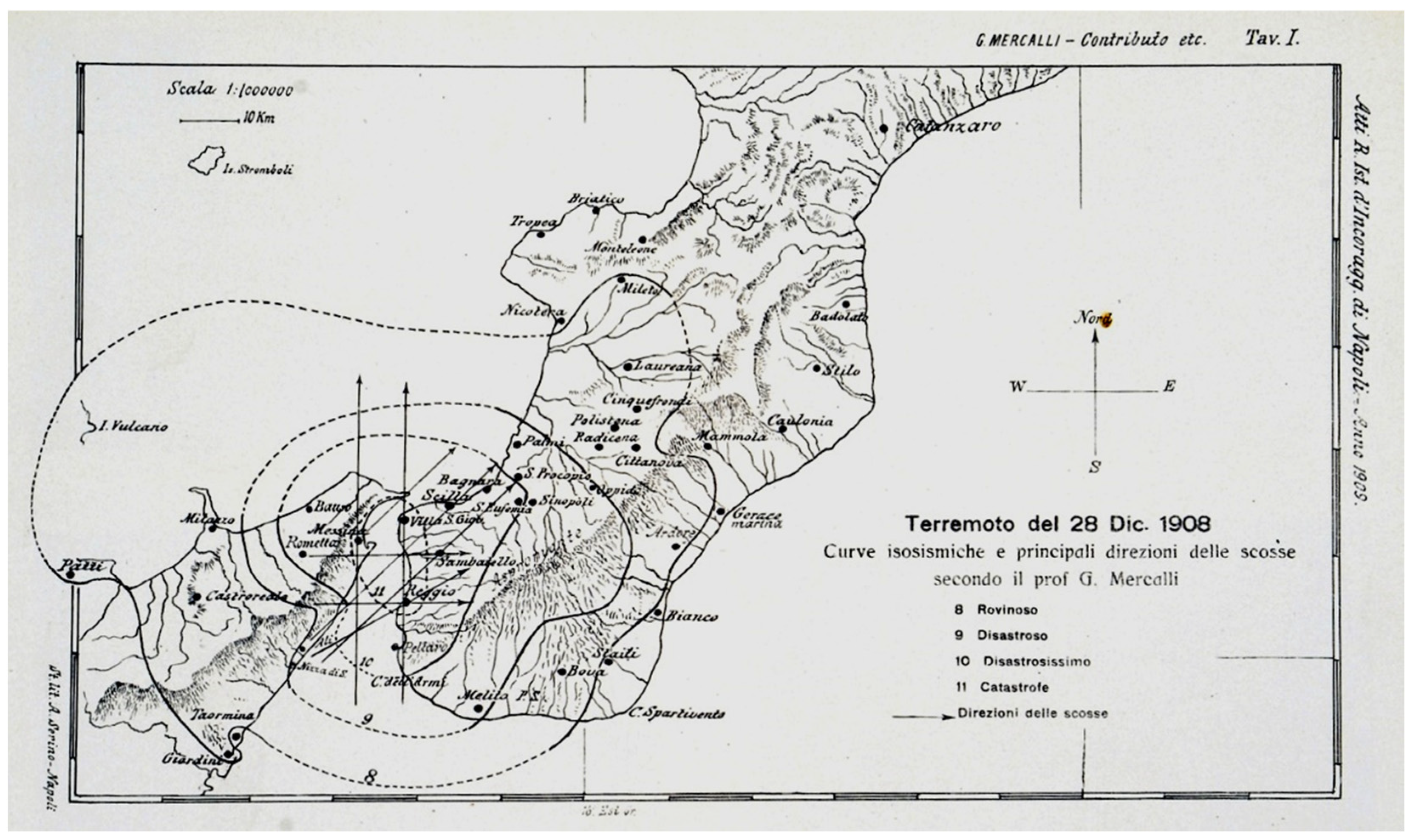
The area of the Messina Strait is located midway of the Calabrian Arc, one of the most seismically active areas in Italian and Mediterranean that had been stricken by earthquakes several times in the past, but not as strong as the earthquake of December 1908. Figure 2 shows the intensity pattern for the 1908 earthquake [16]. Between the main historical seismic events with Me > 5.5, the 31 August 853 and the 6 February 1783 earthquakes need to be mentioned, respectively, with I0 IX-X and I0 VIII-IX [17]. The historical records also report two events, presumably significant, in 91 B.C. (I0 IX-X) and 361 A.D. (I0 X).
2.2. Geological Aspects
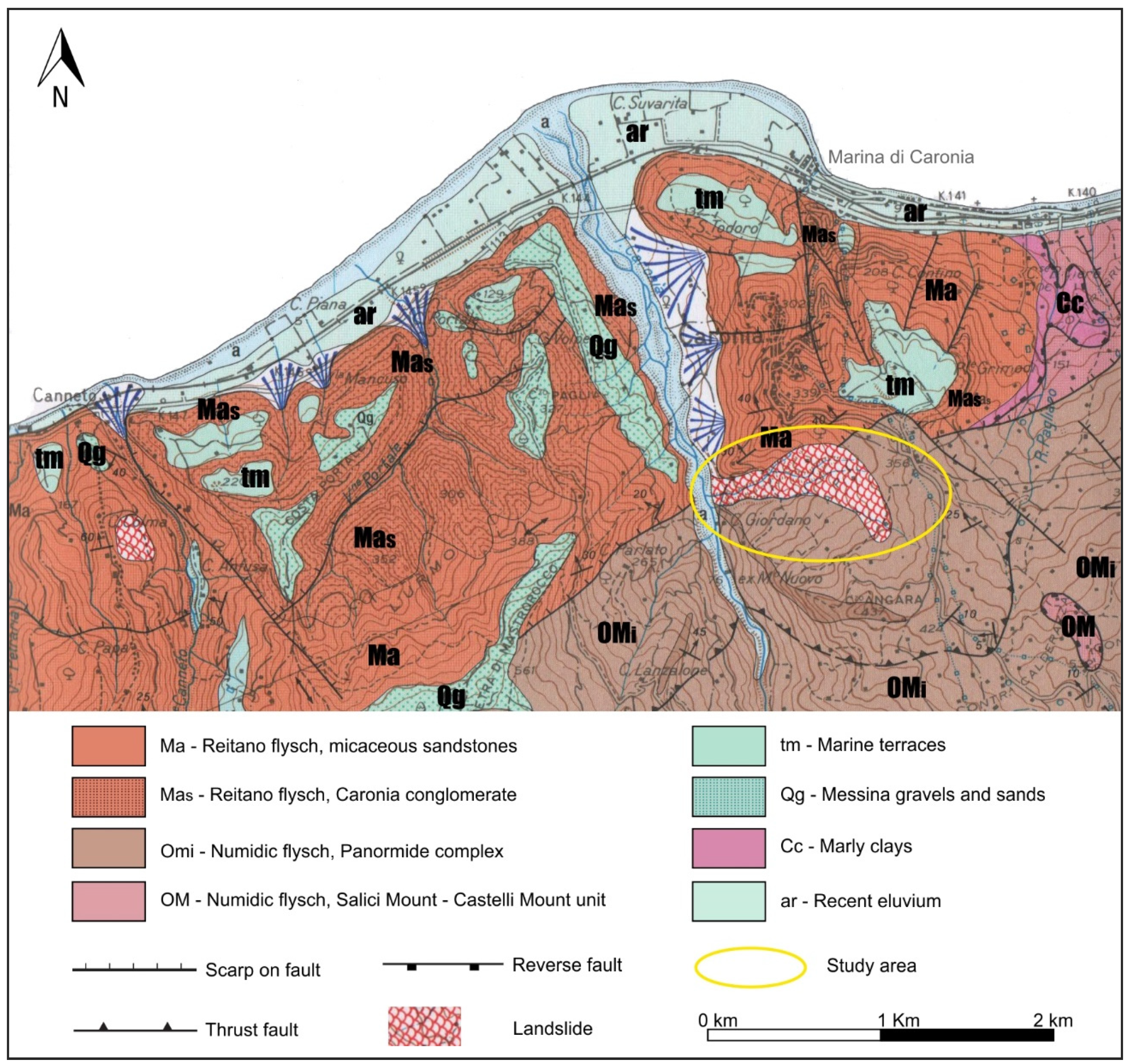
The eastern sector of the Nebrodi Mountains (NE Sicily), a part of the Apennines-Maghrebian orogenic chain, is characterized by a high landslide hazard [18,19]. The study area is characterized by three different geological units (Tardorogene covering, Sicilide complex and Panormide complex), according to the Geological Map of the Messina Province, as shown in Figure 3.
The features of the geological units are reported in the following:
- (a)
- Tardorogene coverings unit—Reitano flysch: alternation of micaceous sandstones, of yellowish or gray-brown color, with intercalations of grayish or greenish marly clays (Ma and Mas in the geological map).
- (b)
- Sicilide complex—Upper scaly clays unit: marly clays and gray-blackish clayey marl with decimetric levels of gray marly limestone and grayish calcarenite (Cc in the geological map); Salici Mount—Castelli Mount unit: numidic flysch, blackish shafts (OM in the geological map) passing upwards to an alternation of brown clays and yellowish quartz arenites with local marly limestone and marl.
- (c)
- Panormide complex—numidic flysch, alternation of siliceous argillites and quartz arenites or quartz osyltites (Omi in the geological map).
In general, it is observed that some portions of the Reitano Flysch appear disarticulated in the outcrop, with fragmented and fractured lithoid layers.
2.3. Investigation Program and Geotechnical Soil Properties
The Regional Department of the Civil Defense put in many efforts in terms of studies and analyses that obtained precious information for a detailed geotechnical characterization of the Caronia area [21].
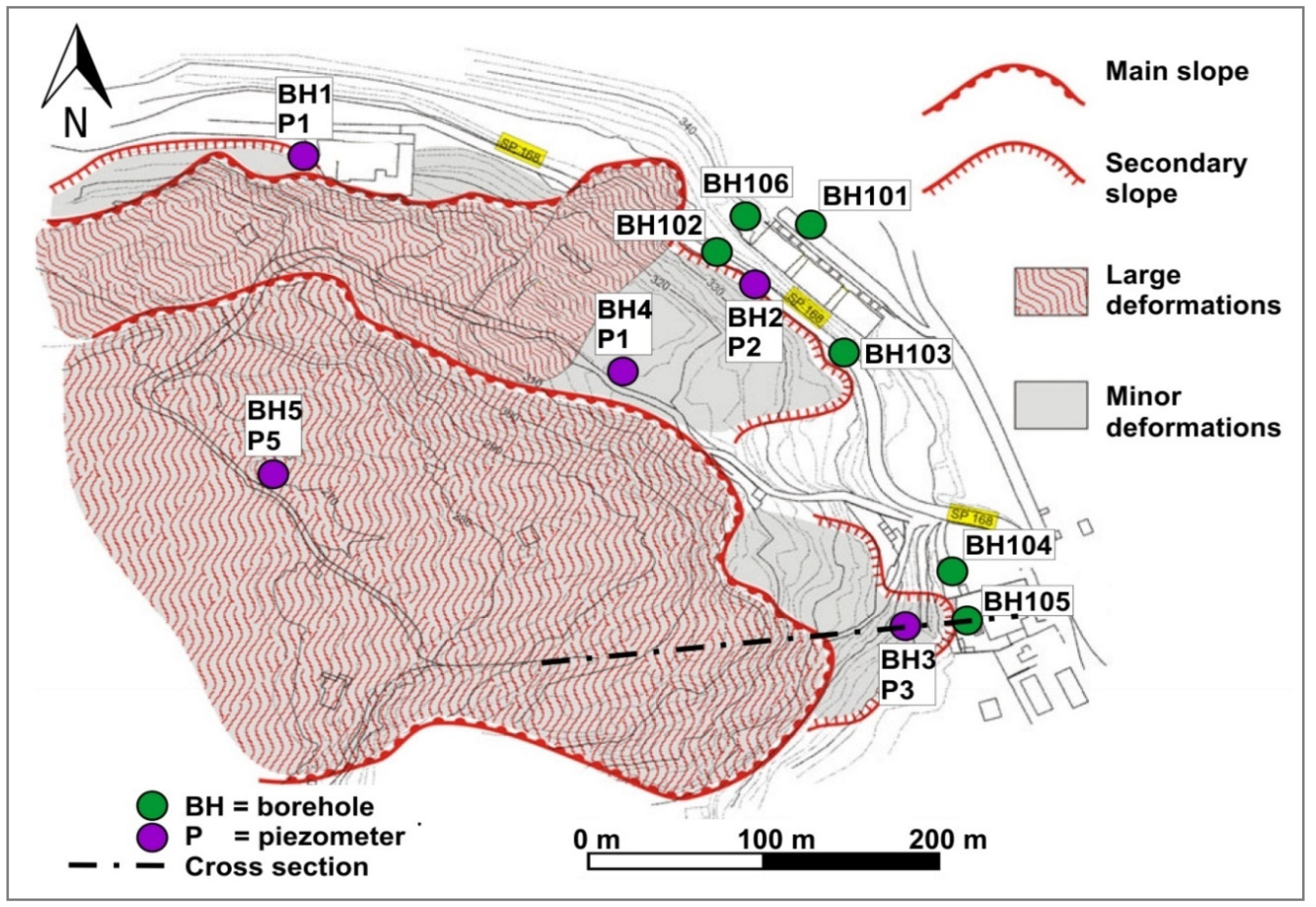
The static and dynamic geotechnical characterization of soils in the Contrada Lineri of Caronia was performed within an investigation test site with a surface of about 13 hectares; Figure 4 shows the layout of test sites with the location of geotechnical boreholes and piezometers.
The study area reached a maximum depth of 30 m. Laboratory tests (moisture content; soil unit weight; specific gravity; grain size analysis; Atterberg limits; direct shear test) were performed on undisturbed samples [22].
To evaluate the geotechnical characteristics of soils, the following in situ and laboratory tests were performed in the area: n. 11 Boreholes, n. 10 Piezometers, n. 5 Inclinometric Measurements, n. 3 Down-Hole tests (DHT), n. 7 Seismic Tomography Tests, n. 2 Multichannel Analysis of Surface Waves (MASW), n. 12 Direct Shear Tests (DST).
Based on of the data available from boreholes (Table 1), soil profiles of the ground beneath the Caronia test sites could be designed. Summarizing the borehole results, it is possible to define four soil classes, namely: plastic structureless clays, brown color structureless clays, gray color structureless clays and argillites. The water level was in the range 8.30–11.20 m.
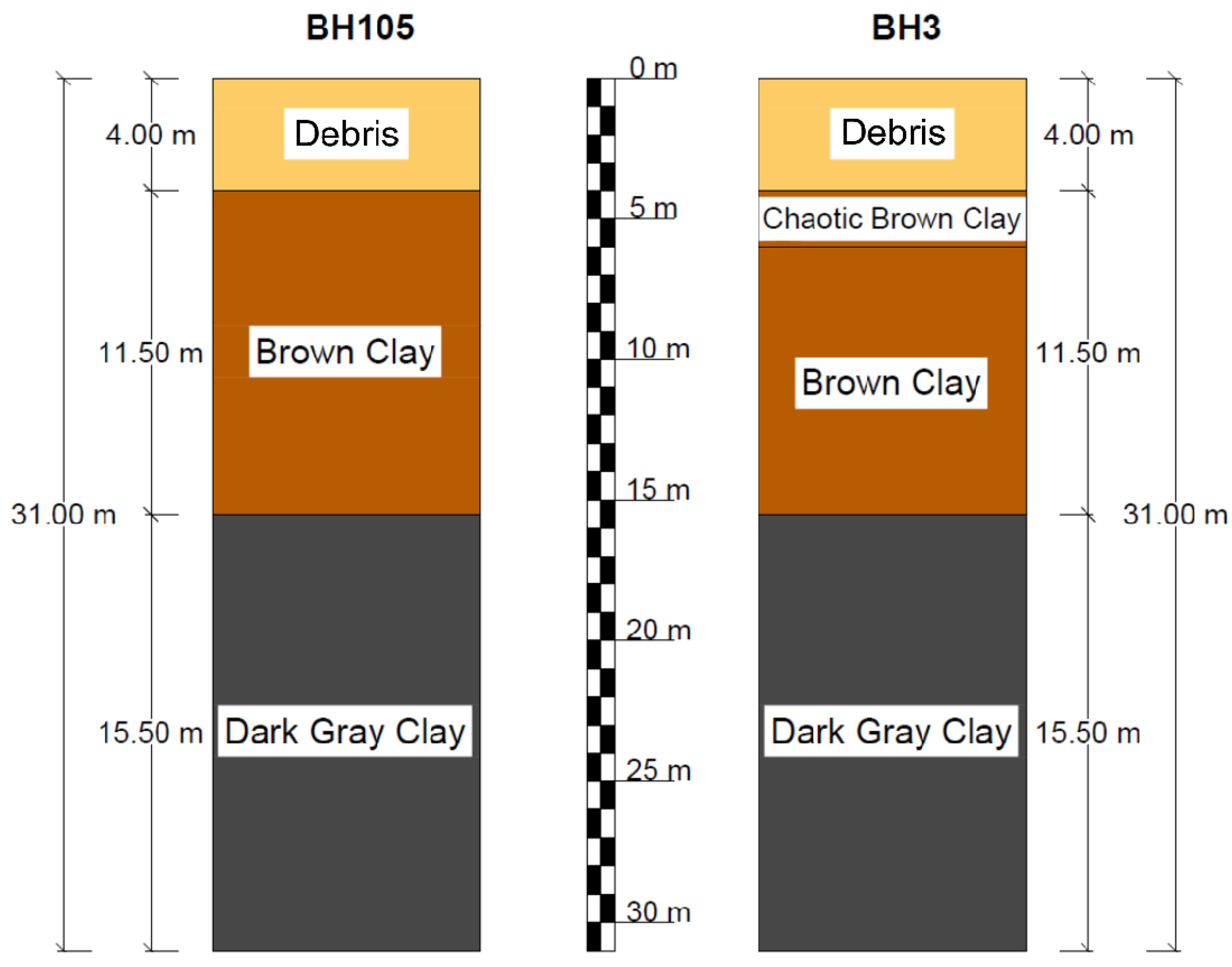
The stratigraphic columns were obtained directly by the study of topographical profiles. This was done by trying to predict as accurately as possible what the soil profile looked like beneath the surface from the information available from the stratigraphic columns, linking corresponding strata with neighboring stratigraphic columns where possible. Once each stratum was completed, the corresponding lithological design was assigned (Figure 5).
Based on the laboratory tests, the typical range of physical characteristics, index properties and strength parameters of the deposits mainly encountered in these areas are reported in Table 2 and Table 3.
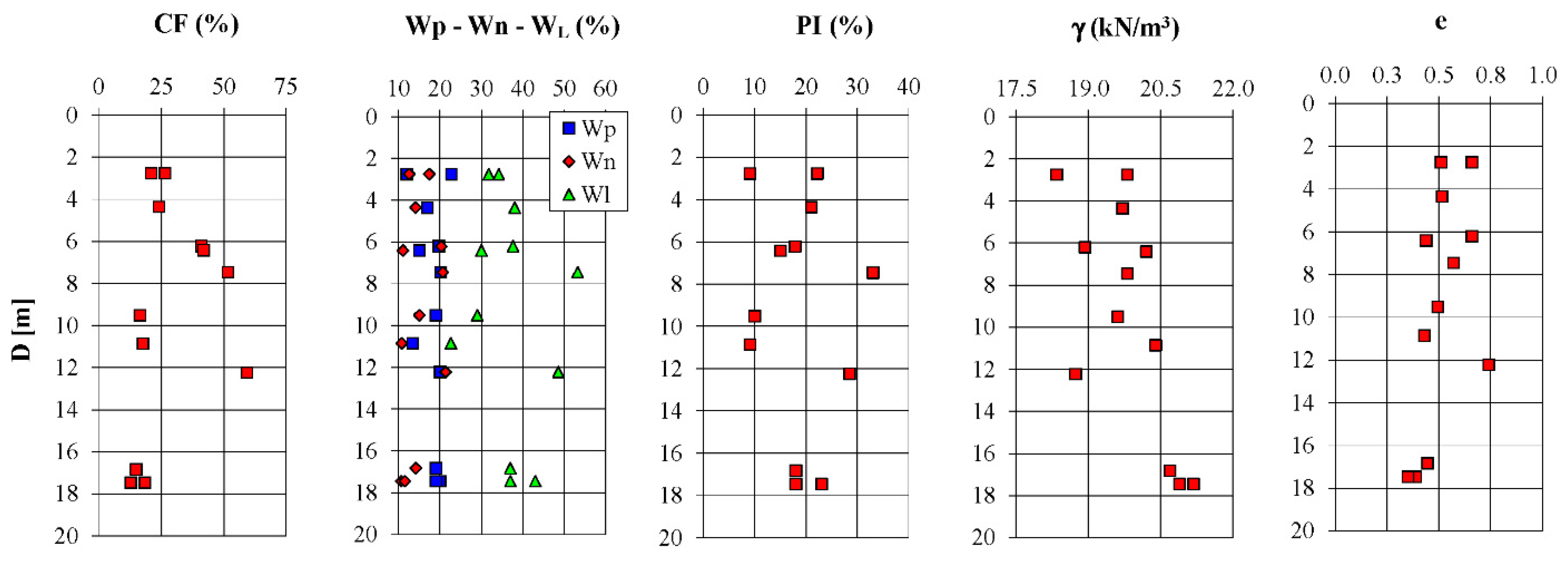
The value (Figure 6) of the natural moisture content wn prevalently ranged between 11–26%, while characteristic values for e (void ratio) ranged between 0.35 and 0.74 for the Caronia test site.
Regarding strength parameters of the deposits mainly (Table 3) encountered in this area, c’ from DST ranged between 2.41kPa and 51.8kPa while φ‘ from DST ranged between 15.8° and 31.6°.
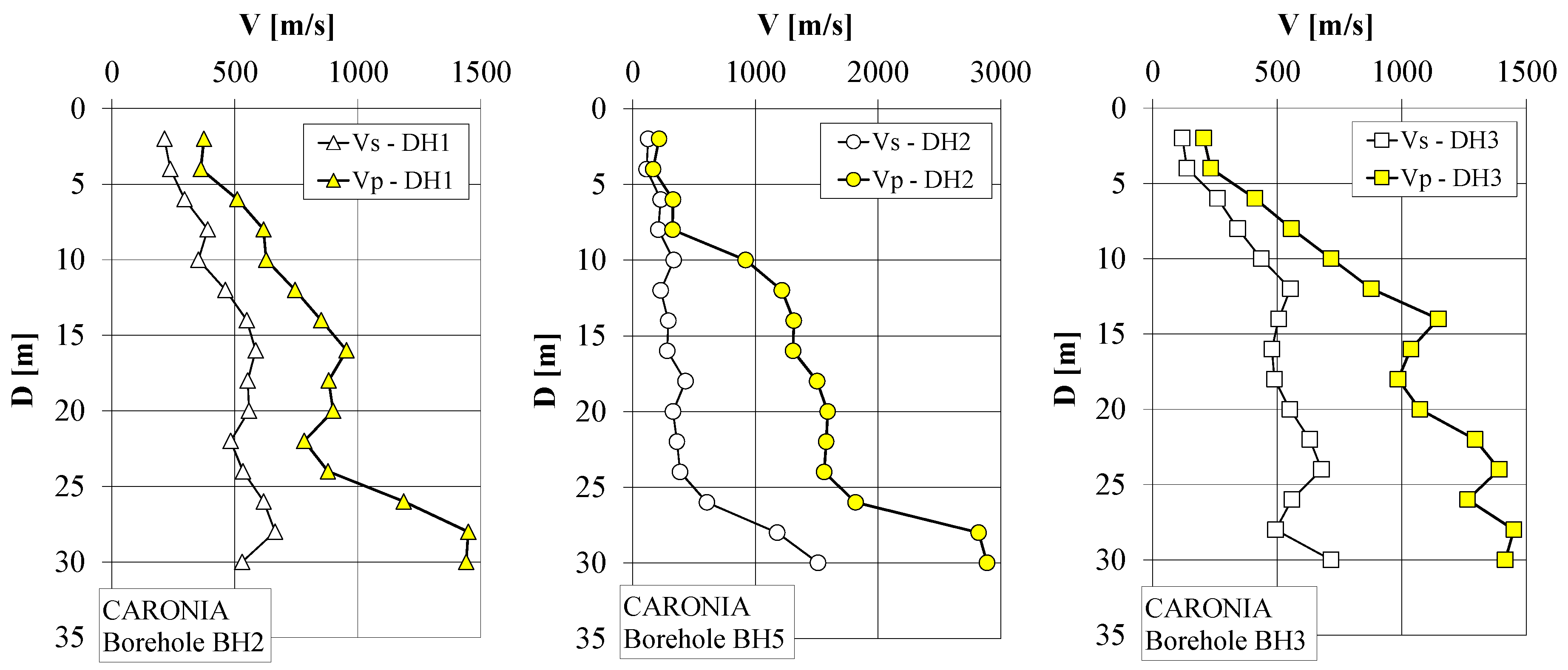
It was also possible to evaluate the small strain shear modulus in the Caronia area by means of the following seismic tests based on Down Hole (DH). In Figure 7, the shear and compression wave velocities are shown against depth.
The shear Vs and compression Vp wave velocities gradually increased with depth. At the depth of about 25–30 m, there was a rapid increase in velocities due to the presence of fractured argillite.
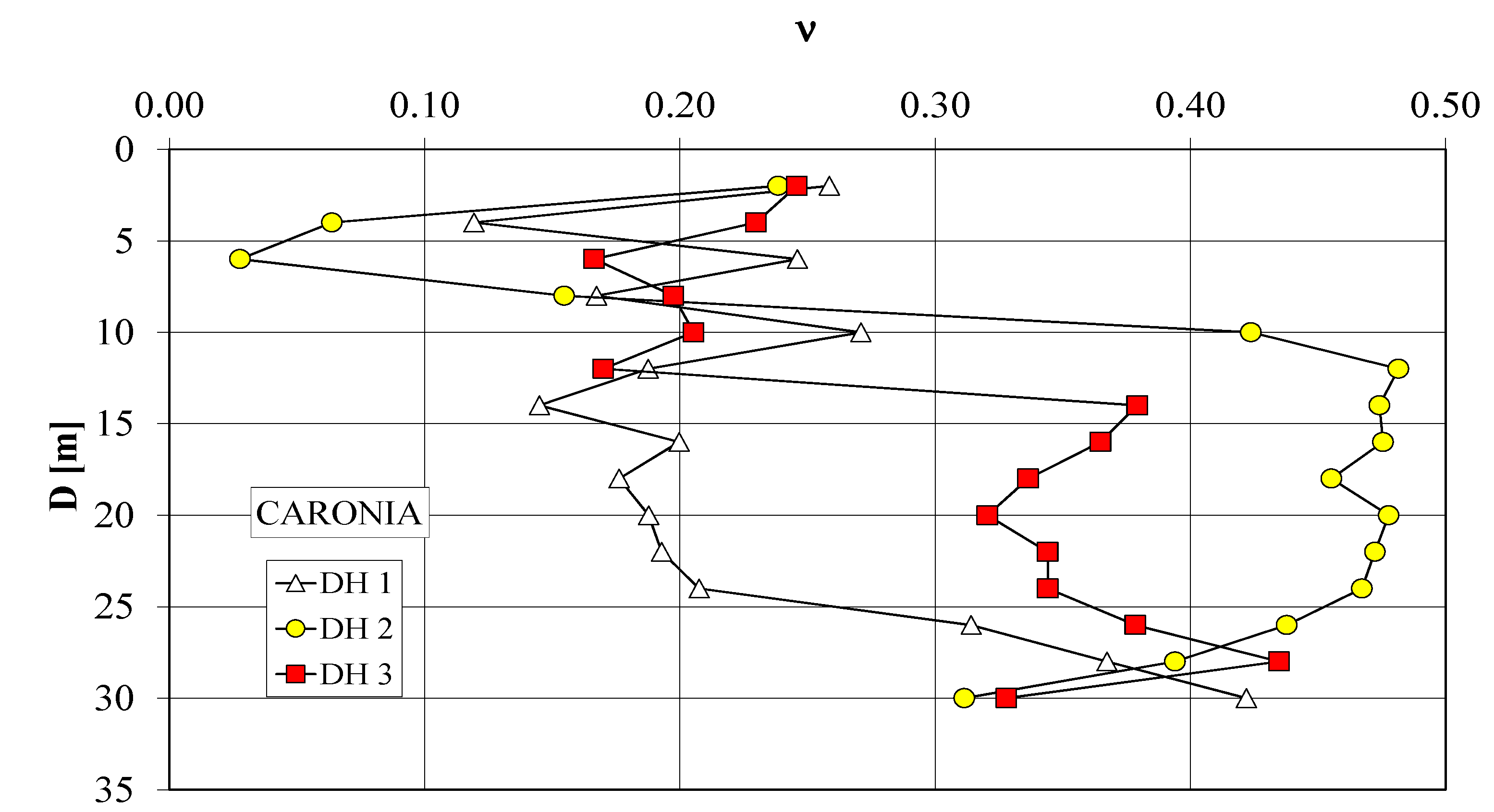
In Figure 8, the dynamic Poisson ratio (ν) variation with depth, obtained from the Down-Hole (DH) test, is plotted to show site characteristics. It is shown that the values oscillate around 0.03–0.48 for DH.
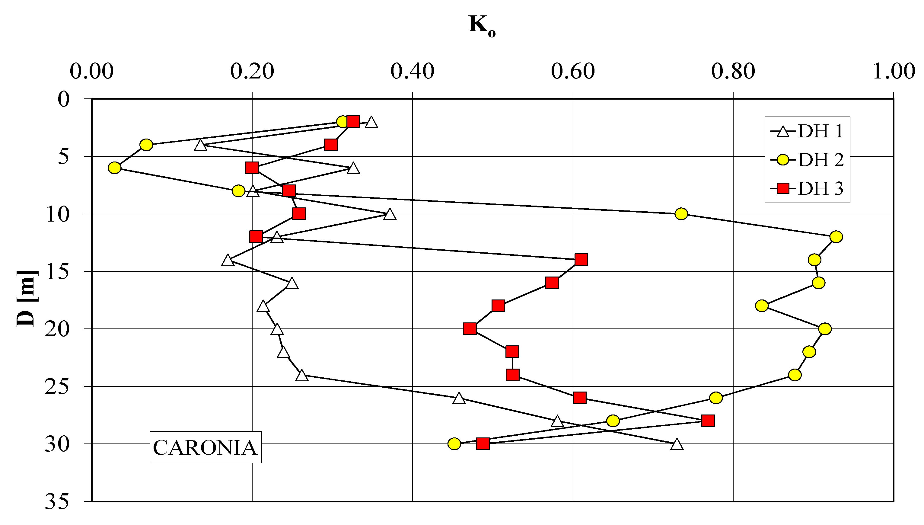
In Figure 9, the coefficient of earth pressure at rest Ko variation with depth, obtained from a Down-Hole (DH) test, is plotted to show site characteristics. It is shown that apart from the top 5 m, the values oscillate around 0.07–0.93 from DH.
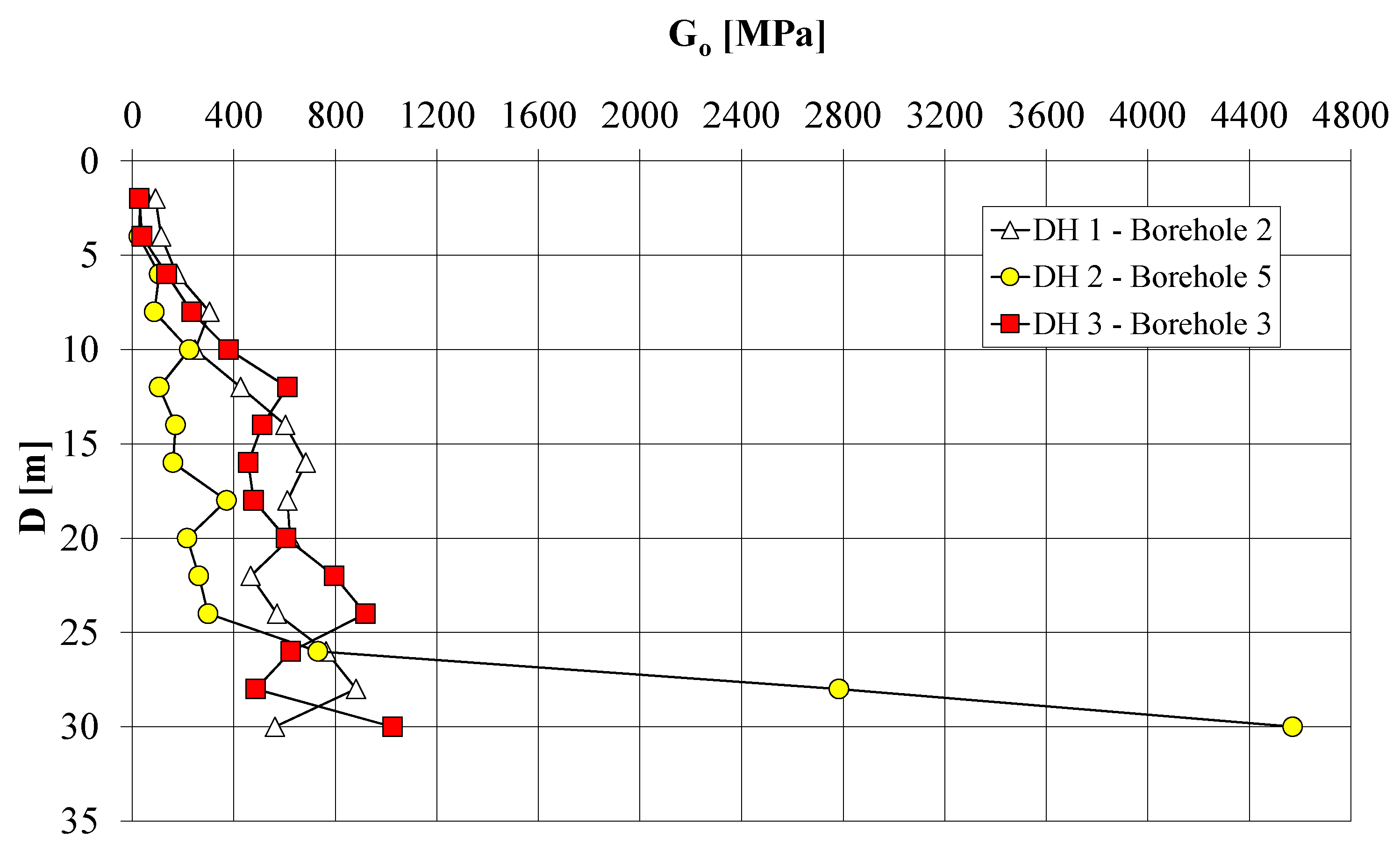
A comparison between the shear modulus values of Go obtained from in situ tests performed on the area under consideration is shown in Figure 10. The down-hole tests performed in the Caronia area show Go values increasing with depth. Very high values of Go were obtained for depths greater than 25 m in borehole 5. According to these data, it was possible to assume Go values oscillating around 50–1000 MPa.
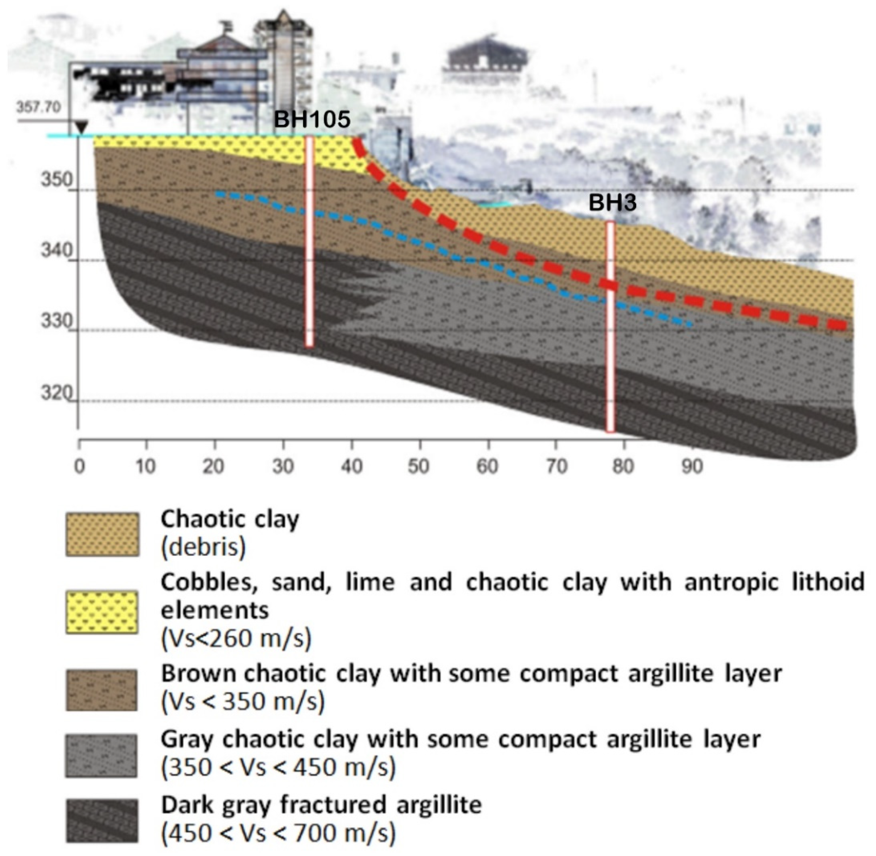
Figure 11 shows a particular cross-section with the geological and geotechnical information from which we note the presence of predominantly clayey material with Vs values included in the range 200–700 m/s. The borehole BH105 was performed along with the stable share of landslide cross-section, while the borehole BH3 was performed along with the unstable share of landslide cross-section. These two boreholes allow us to definition the geotechnical characteristics of the Caronia landslide.
3. Site Response Analysis
3.1. Seismic Input Motion and Soil Dynamic Properties
This work takes into specific consideration the site effects’ role on the predictable ground motions in the Caronia area. More precisely, when it comes to site effects, we generally refer to the influence of the first 40–50 m of near-surface stratigraphy on the seismic response of the soil. Great importance is also given to the source and the path effects [23].
Seven different inputs were used, consisting of six synthetic seismograms related to the Messina and Reggio Calabria 1908 earthquake (Bottari et al. [24]; Tortorici et al. [25]; Amoruso et al. [26]; DISS Aspromonte Est; DISS Gioia Tauro; DISS Messina Strait) and one related to the 1693 Catania scenario earthquake [27,28,29,30]. The seismograms were scaled to the (Peak Ground Acceleration) PGA = 0.176 g provided by the Italian Code NTC 2018 for the site.
Soil dynamic properties were also taken into account in the numerical analyses through the stiffness attenuation G/Go-γ and damping ratio evolution with strain D-γ curves [31] related to similar materials of the same area [32,33].
The dependency of the shear modulus and damping ratio on shear strain level was obtained by interpolating the experimental resonant column tests (RCT) data by Yokota et al.’s [34] equation to the experimental data points. For the Caronia area, the following equations were used:
to describe the shear modulus decay with shear strain level, in which G(γ) = strain dependent shear modulus, γ = shear strain and α, β = soil constants, with
to describe the inverse variation of damping ratio with respect to the normalized shear modulus, in which D(γ) = strain dependent damping ratio, γ = shear strain and η, λ = soil constants.
The values of α, β and of η, λ are reported in Table 4.
3.2. Numerical Analyses
To evaluate morphological and stratigraphic effects, 1-D and 2-D equivalent-linear site response analyses were performed. Several techniques were proposed for the assessment of these effects; by comparing the results from experimental estimates of local site amplification effects and numerical analyses, it was demonstrated that 1-D numerical modeling can underestimate the amplification of ground motion and cannot account for resonant frequencies every time [35]. In these cases, the use of 2-D numerical methods is almost essential to obtain a more realistic estimate of the seismic response [36].
The 1-D analyses were carried out in three vertical profiles extracted from the 2-D cross-section, located in this way: (1) the first behind the crest of the slope, (2) the second at the crest of the slope, (3) the third at a point downstream sufficiently far from the foot of the slope.
The 1-D analyses were performed by the EERA (Equivalent-Linear Earthquake Site Response Analysis) code [37] that permits performance of frequency domain analyses for equivalent linear stratified sub-soils. The same elaborations were also carried out through the QUAKE/W code to obtain a calibration of the two codes and be able to proceed subsequently with the 2-D analyses. A comparison of results from these two different codes is a good way of validating the formulation and implementation of the work. The EERA model was simulated in QUAKE/W as a column of elements where the base of the column is fixed. This has the effect of the earthquake motion being applied at the column base. The sides of the column are fixed in the vertical direction, which ensures that all the motion is in the horizontal direction only, an assumption inherent in the EERA 1-D formulation.
The 2-D analyses were performed by the QUAKE/W [38] code based on a finite element formulation with a direct integration scheme in the time domain. “Direct integration” means no transformation of the equations into the frequency domain is required. Then, the motion equations are solved directly using a finite-difference time-stepping procedure.
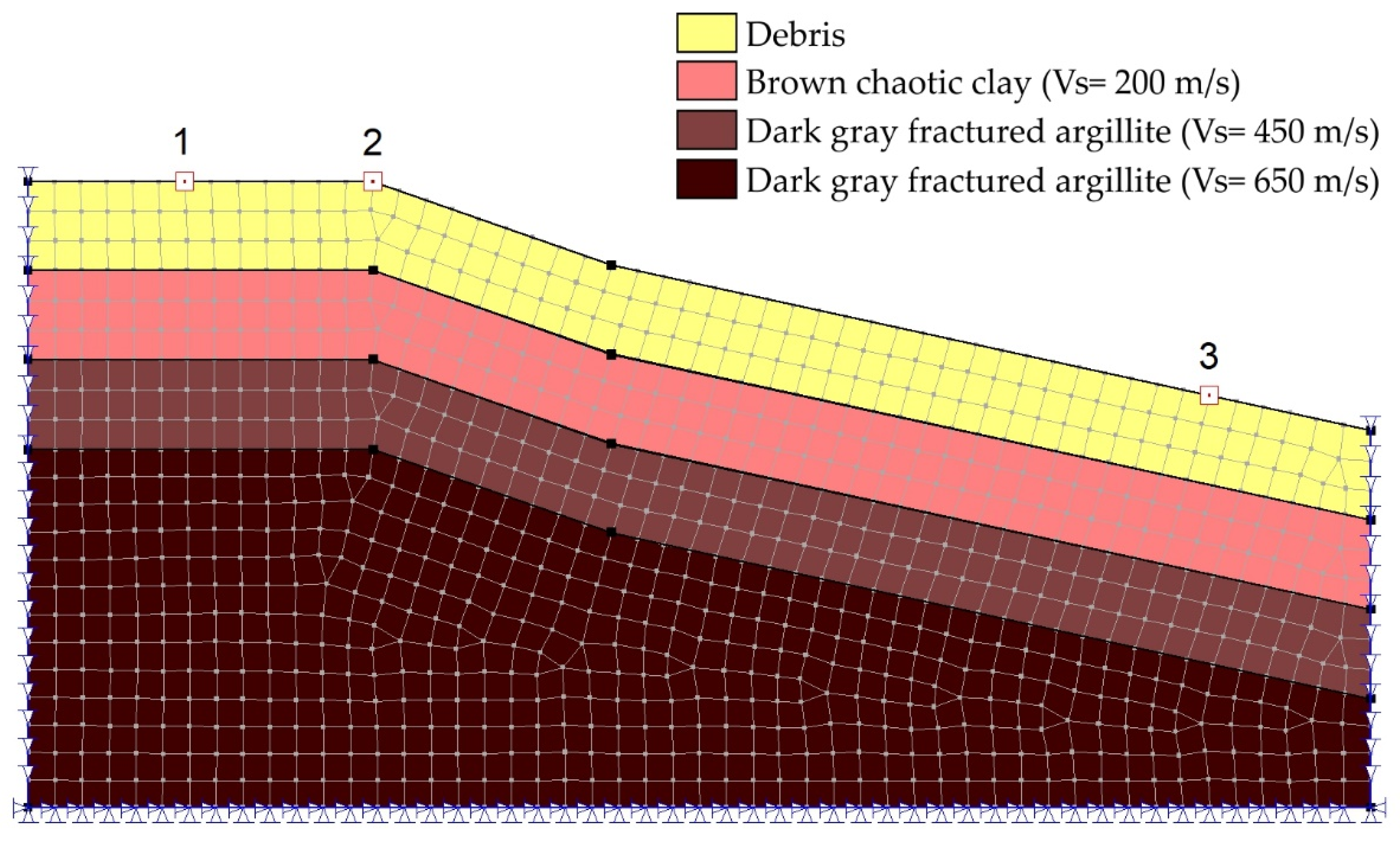
Figure 12 shows the cross-section used for the finite element analyses; the three-surface points monitored by 1-D and 2-D analyses were also indicated in the same figure.
3.3. 1-D Analysis
For complex geometries, it is very important to perform dynamic analyses by different codes, and in particular through 2-D codes that can catch some aspects that 1-D codes cannot catch.
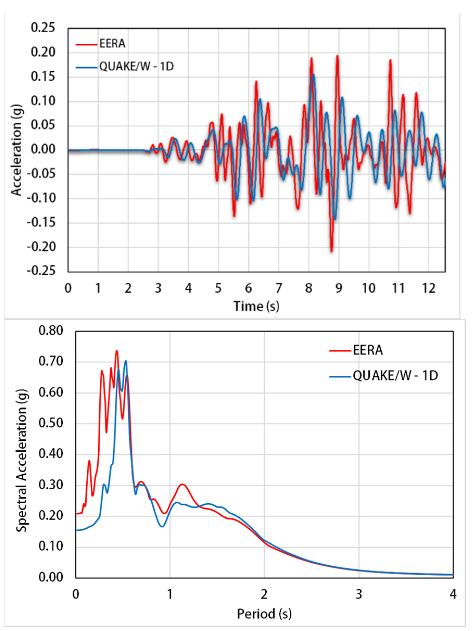
The 1-D analyses performed by EERA and QUAKE/W codes, for the seven inputs, show similar values of PGA for points 1 and 2 (behind the crest point and crest point) [39]. The following figures show in red and blue, respectively, the EERA and QUAKE/W results in terms of acceleration time history and spectral acceleration. In particular, Figure 13, Figure 14 and Figure 15 show the 1-D analysis results for the Amoruso et al. [26] input, and the results have been summarized in the Table 5. Results obtained for points 1 and 2 show values of the stratigraphic soil amplification factor of about 1.30 using the EERA code and of about 1.20 using the QUAKE/W code. For point 3, there is no significant stratigraphic soil amplification.
Table 6 shows, for the same points, the results of 1-D analysis carried out by the seismograms for the Bottari et al. [24], Tortorici et al. [25], DISS Messina Strait, DISS Gioia Tauro, DISS Aspromonte Est, and 1693 Catania Earthquake.
Results obtained for points 1 and 2, show maximum values of the stratigraphic soil amplification factor of about 1.45 using EERA code and of about 1.50 using QUAKE/W code. While for point 3 results show a slight stratigraphic soil amplification of about 1.10.
3.4. 2-D Analysis
In addition to 1-D results, a 2-D analysis of the slope was performed using QUAKE/W code. The importance of the comparison for the same case study between 1-D and 2-D analyses is well known and it plays an important role not only for a sloping ground area but, in general, for geometric irregularities. An example is reported by Elton et al. [40] by analyzing the stability of an earth dam affected by a seismic action. Authors compared two methods for calculating the peak dynamic shear stress that occurs in embankments during an earthquake based on 1-D analyses performed using the SHAKE code [41] and on 2-D analyses carried out using the FLUSH code [42].
Furthermore, an accurate evaluation of the PGA also plays a very important role in slope stability in seismic conditions. In fact, the influence of the PGA on the identification of the critical slip surface under seismic loading, and, consequently, on the safety factor of the slope, is well known. In addition, the knowledge of the response time history and of the PGA can be very helpful in the study of permanent displacements, as recently reported by Ji at al. [43,44].
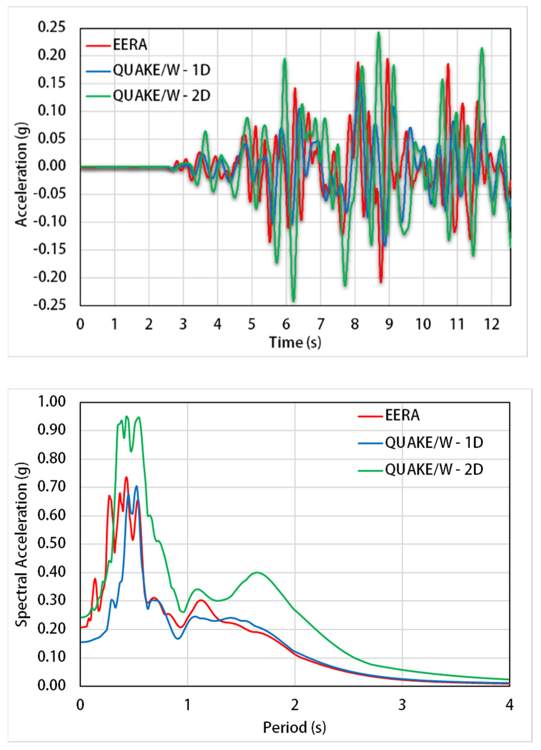
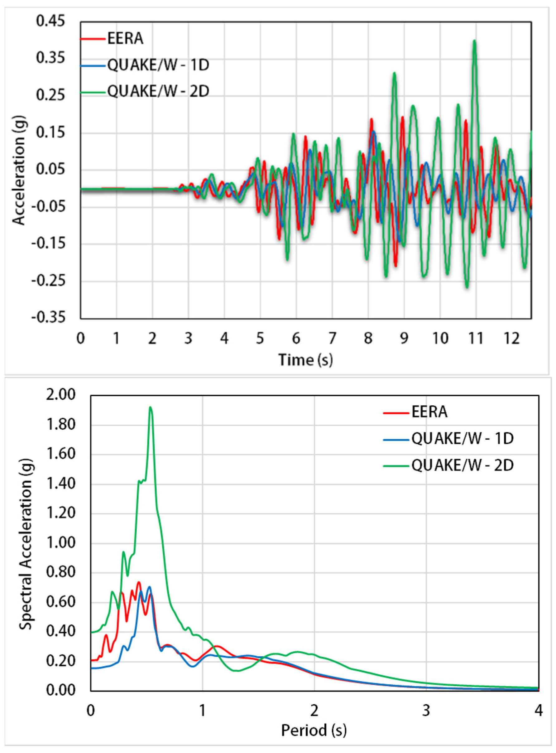
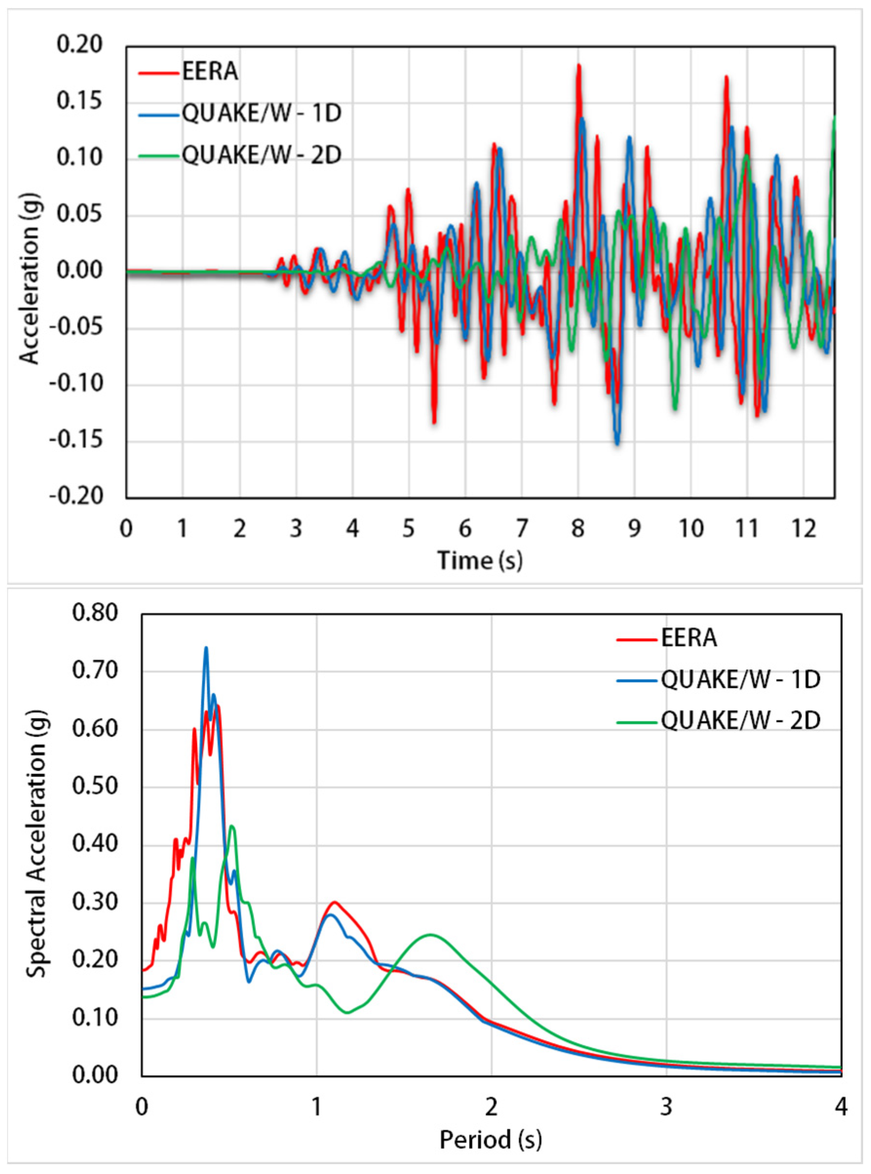
The following figures show in red, blue and green, respectively, the EERA, QUAKE/W 1-D and QUAKE/W 2-D result in terms of acceleration time history and spectral acceleration. Figure 16 shows the surface maximum acceleration along the 2-D modelization through the QUAKE/W code.
3.5. Topographic Effects
It is well known that the topography affects the responses at the free surface by complicated cycles of amplification and de-amplification. In general, the responses are amplified at the upper surface of slopes and attenuated at their base.
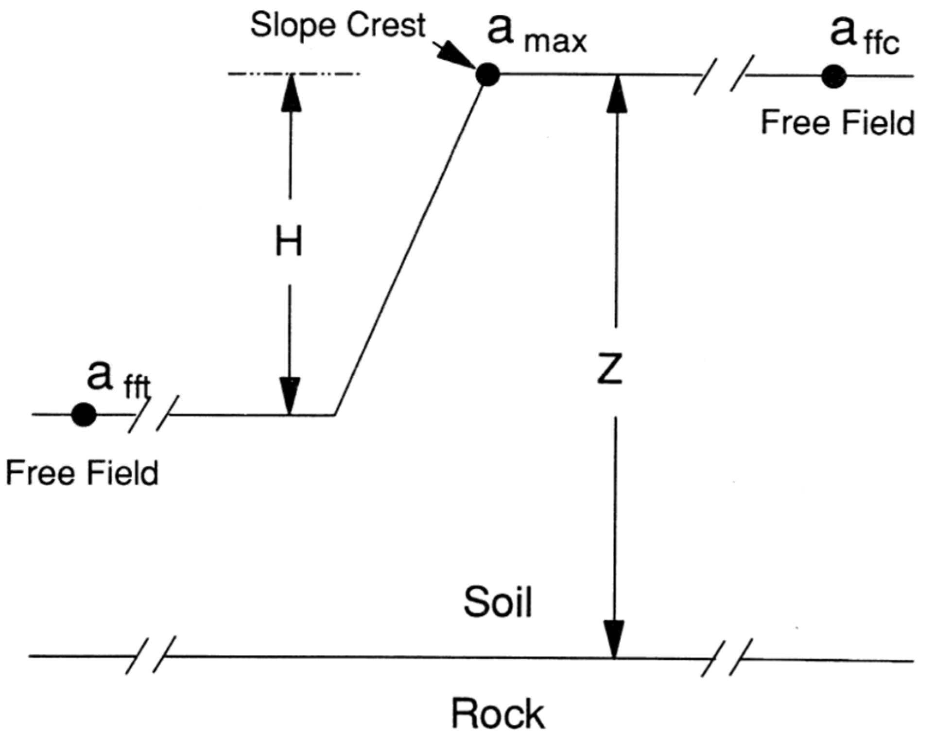
Among the most important study of topographic amplification, we recall the experience of Ashford and Sitar [45,46] and Ashford et al. [47], related to the seismic response of steep natural slopes. In this study, the site response was characterized by maximum acceleration at various locations as follows (Figure 20):
- -
- afft, the maximum free field acceleration in front of the toe;
- -
- affc, the maximum free field acceleration behind the crest see Equation (4);
- -
- amax, the maximum crest acceleration.
In this study, the topographic and site amplification were treated separately in order to determine the contribution of the different factors; therefore, three measures of amplifications were computed: At—Equation (3)—“topographic amplification,” the amplification of the free field motion at the crest; As—Equation (4)—“site amplification,” the amplification due to the natural frequencies of the site; Aa—Equations (5) and (6)—“apparent amplification,” the apparent amplification of the motion between the base and the crest. The proposed parameters were obtained as follows:
Aa = (1 + At)(1 + As) − 1
The results of numerical analyses carried out for the input (Bottari et al., [24]; Tortorici et al., [25]; Amoruso et al., [26]; DISS Aspromonte Est; DISS Gioia Tauro; DISS Messina Strait), and based on the Ashford approach, are shown in the Table 9.
Results show a topographical amplification coefficient, given by 1 + At greater than 1.20, while the same coefficient given by NTC 2018 for the study area is equal to 1.20.
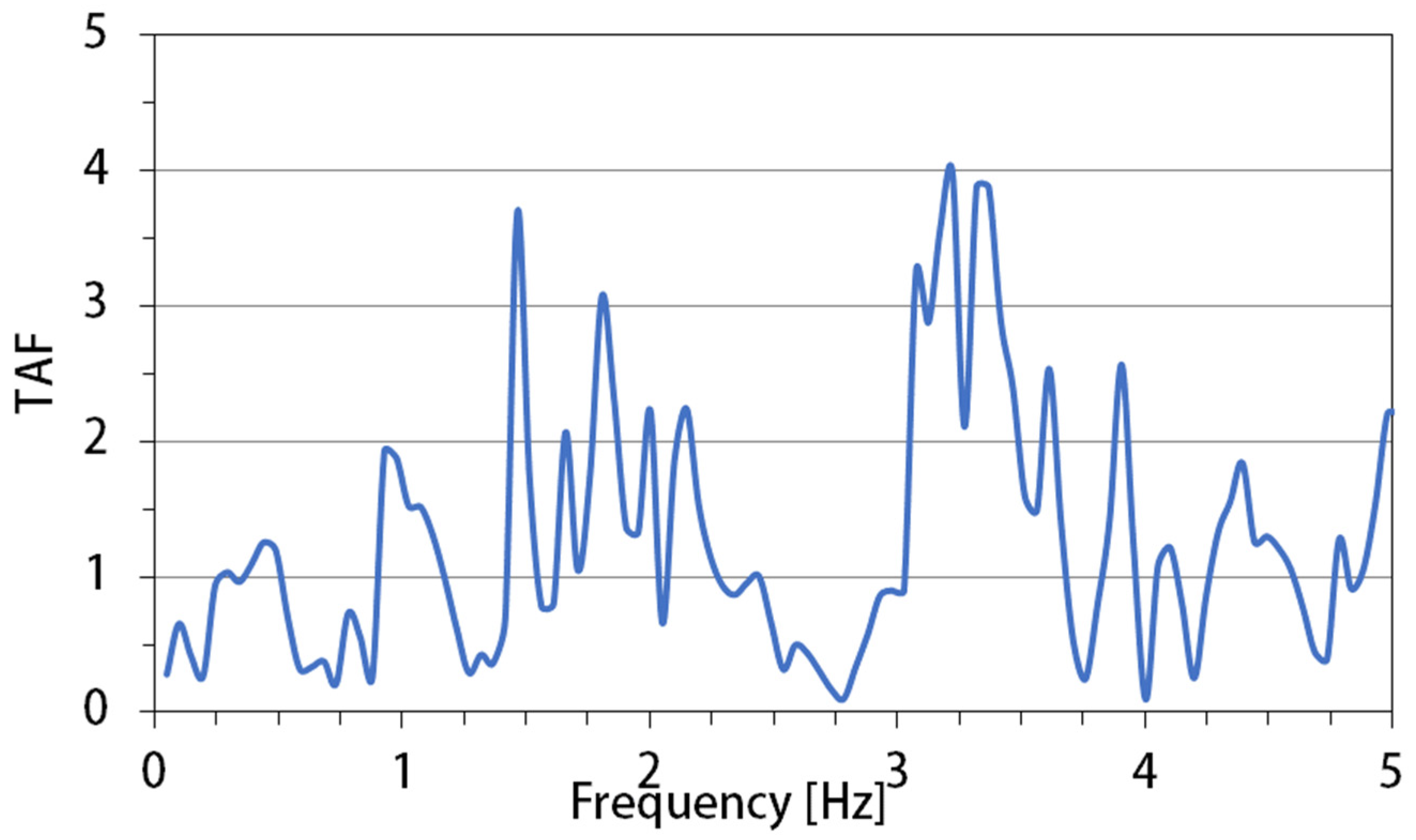
Topographic amplification can be also measured by the ratio between the Fourier spectrum of the seismogram at the crest (10 m away) and the Fourier spectrum of the free field seismogram behind the crest (250 m away). This is the so-called TAF (Topographic Aggravation Factor) which is defined in the frequency domain, after Kallou et al. [48].
Figure 21 shows the Topographic Aggravation Factor (TAF), after the Kallou et al. [48] approach, for the Amoruso et al. [26] input. Results show values of TAF reaching on average about 1.45 in the frequency range f of 1–5 Hz.
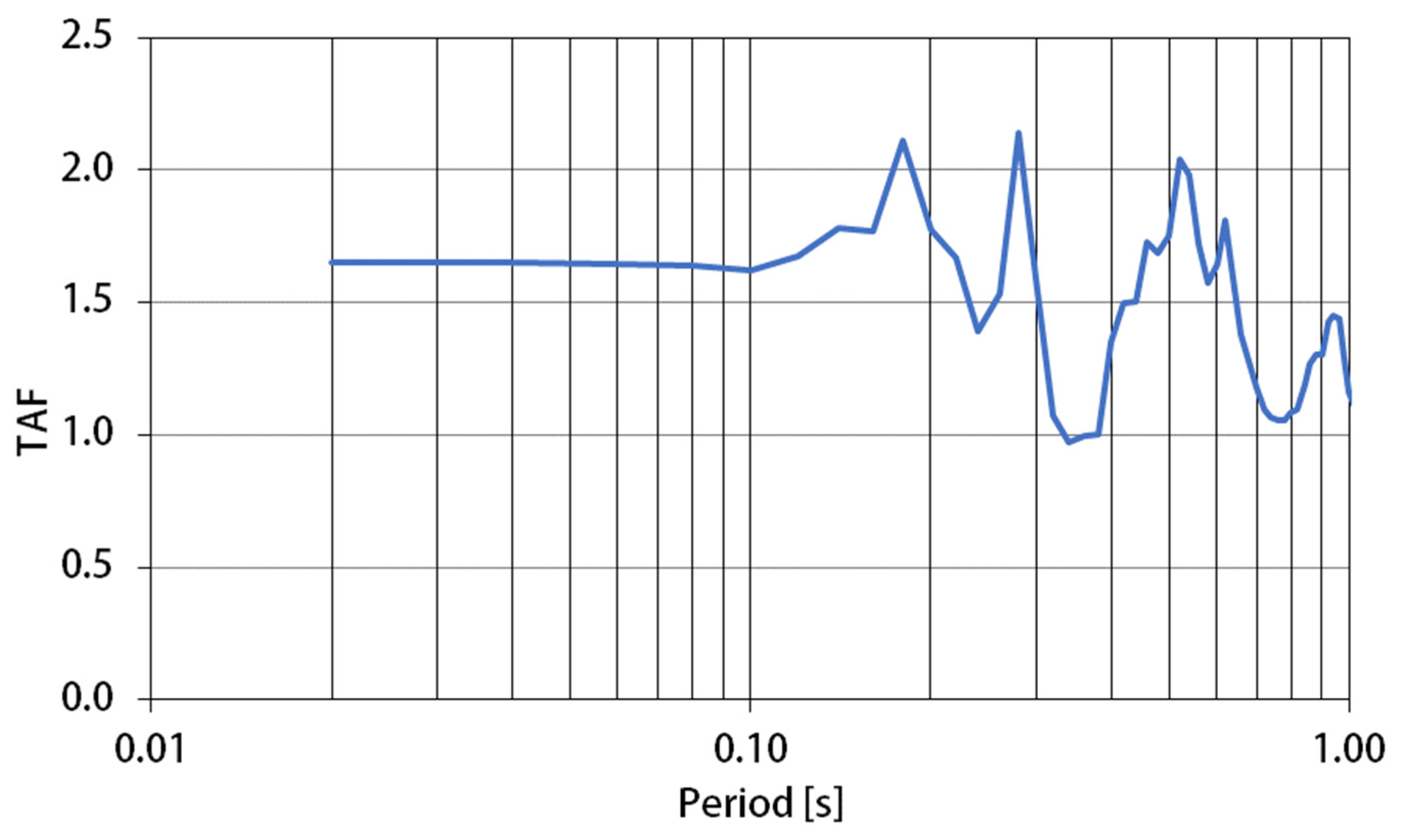
The topographic amplification can be also evaluated in the time domain following the approach proposed by Bouckovalas and Kouretzis [49] in terms of the (2-D)/(l-D) ratio of elastic response spectra obtained at the crest. Figure 22 shows the Topographic Aggravation Factor (TAF) after the Bouckovalas and Kouretzis [49] approach for the Amoruso et al. [26] input. In this case, results show high values of TAF, reaching on average about 1.42 for the period range T of 0.20 to 1.0 s. Obtained values are in agreement with large amplifications obtained for similar studies performed on ridges, slopes and valleys.
4. Discussion and Conclusions
The study of the response of a subsoil subjected to seismic actions is often conducted for different purposes. It allows the prediction of permanent soil deformations and the quantification of the risk of instability phenomena, such as landslides or liquefaction triggering.
In this paper, a study on the evaluation of the topographic effects for a slope in the Tyrrhenian area of Southern Italy has been carried out. Detailed geotechnical characterization was also carried out by in situ and laboratory tests. The laboratory tests performed in the static field made it possible to evaluate the mechanical characteristics of the soil, allowing to obtain the fundamental parameters as a function of depth such as unit weight, moisture content, Atterberg limits, void ratio, porosity and degree of saturation; moreover, through direct shear tests it was possible to obtain the values of the cohesion and the angle of shear resistance. The laboratory tests performed in the dynamic field allowed for evaluating the non-linear behavior of soils in terms of stiffness attenuation with strain G/Go-γ and the damping ratio evolution with strain D-γ. Moreover, the results obtained through the Down Hole (DH) tests made it possible to derive the trend with the depth of the shear wave velocity and other parameters such as the Poisson ratio and the coefficient of earth pressure at rest.
The definition of seismic action was based on synthetic seismograms related to the 1908 Messina and Reggio Calabria earthquake and the 1693 Val di Noto earthquake.
A numerical model based on the 1-D EERA and 2-D QUAKE/W codes was performed for the slope model in the Caronia area, subjected to vertically propagating in-plane shear waves (Vs waves). Results show that stratigraphic amplification and topographic amplification effects were found to interact, suggesting that to accurately predict topographic effects the two effects should not be always handled separately.
1-D computer codes have been used to model the equivalent-linear earthquake site response analyses of layered slope deposits, as generally performed by professionals. Because the slope is moderate (average slope angle is i = 22°), a 1-D response analysis, often used by professionals, was the first step of the study, as indicated by the provisions of national and international building codes. Besides, the local seismic response analysis has been also performed in greater detail using a counted 2-D simple model. Results show amplification of the seismic motion using initially the 1-D code. Besides, by performing the 2-D analysis, further amplification of the seismic acceleration at the crest of the slope was found. By the numerical analyses, three points in the slope cross-section were monitored as follows: point 1 located behind the crest of the slope; point 2 located at the crest of the slope; point 3 downstream sufficiently far from the foot of the slope. This result is in agreement with the Ashford and Sitar [46] approach, as shown in Table 8, where the values of the topographic amplification are presented. An average value of the topographic amplification At = 0.22 was observed, with a maximum value of At = 0.65 using as an input motion the Amoruso et al. [26] seismograms related to the Messina and Reggio Calabria 1908 earthquake.
Comparing 1-D with 2-D results, the stratigraphic site amplification and the Topographic Aggravation Factor (TAF) were also computed. The evaluation of the Topographic Aggravation Factor (TAF), after the Kallou et al. [48] approach, shows values of TAF reaching on average about 1.45 in the frequency range f of 1–5 Hz. The evaluation of the Topographic Aggravation Factor (TAF) following the approach proposed by Bouckovalas and Kouretzis [49]) shows values of TAF reaching on average about 1.42 for the period range T of 0.20 to 1.0 s.
Concerning the Italian Technical Building Code [10], it should be emphasized that the Code identifies four different topographic categories, each of which is associated with a value of the topographic amplification factor St, with a maximum value of St = 1.40 in the case of slopes with an inclination greater than 30°. In the case of a slope inclination less than 30°, as in the Caronia area, the NTC 2018 provides a maximum value of the topographic amplification factor St = 1.20. Therefore, the provisions of the Code NTC 2018 predict rather moderate effects compared to those predicted by the 2-D analyses.
The aim of the study is that it will form a basis for the design of works in the Caronia area and can provide a basis for professional works.
Author Contributions
A.C., A.F., S.G. and A.P. contributed equally to design the research, process the corresponding data, draft, organize and finalize the paper. All authors have read and agreed to the published version of the manuscript.
Funding
This research received no external funding.
Institutional Review Board Statement
Not applicable.
Informed Consent Statement
Informed consent was obtained from all subjects involved in the study.
Data Availability Statement
All data and codes performed during the study appear in the paper.
Conflicts of Interest
The authors declare no conflict of interest.
References
- EC8. Design Provisions for Earthquake Resistance of Structures, Part 1-1: General Rules-Seismic Actions and General Requirements for Structures. prEN 1998-5; European Committee for Standardization: Brussels, Belgium, 2000. [Google Scholar]
- Boore, D. The effect of simple topography on seismic waves: Implications for the accelerations recorded at Pacoima Dam, San Fernando Valley, California. Bull. Seismol. Soc. Am. 1973, 63, 1963–1973. [Google Scholar]
- Bouchon, M. Effect of topography on surface motion. Bull. Seismol. Soc. Am. 1973, 6, 615–632. [Google Scholar]
- Sepúlveda, S.; Murphy, W.; Jibson, R.; Petley, D. Seismically induced rock slope failures resulting from topographic amplification of strong ground motions: The case of Pacoima Canyon California. Eng. Geol. 2005, 80. [Google Scholar] [CrossRef]
- Assimaki, D.; Kausel, E.; Gazetas, G. Soil-dependent topographic effects: A case study from the 1999 Athens earthquake. Earthq. Spectra 2005, 21, 929–966. [Google Scholar] [CrossRef]
- Celebi, M. Topographical and geological amplifications determined from strong-motion and aftershock records of the 3 March 1985 Chile earthquake. Bull. Seism. Soc. Am. 1987, 77, 1147–1167. [Google Scholar]
- Geli, L.; Bard, P.Y.; Jullien, B. The effect of topography on earthquake ground motion: A review and new results. Bull. Seismol. Soc. Am. 1988, 78, 42–63. [Google Scholar]
- Wang, Y.; He, J.; Yonghong, L.; Cao, S.; He, Z. Seismic monitoring of a slope to investigate topographic amplification. Int. J. Geohazards Environ. 2015, 1, 101–109. [Google Scholar] [CrossRef]
- Glinsky, N.; Bertrand, E.; Régnier, J. Numerical simulation of topographical and geological site effects. Applications to canonical topographies and Rognes Hill, South East France. Soil Dyn. Earthq. Eng. 2018, 116, 620–636. [Google Scholar] [CrossRef]
- NCT 2018—Ministry of Infrastructure and Transport. Decree of the Ministry of Infrastructure and Transport (MIT) of the 01/17/2018; Ministry of Infrastructure and Transport: Rome, Italy, 2018.
- Rovida, A.; Locati, M.; Camassi, R.; Lolli, B.; Gasperini, P. Catalogo Parametrico dei Terremoti Italiani (CPTI15), Version 2.0; Istituto Nazionale di Geofisica e Vulcanologia (INGV): Rome, Italy, 2019. [CrossRef]
- Meschis, M.; Roberts, G.P.; Mildon, Z.K.; Robertson, J.; Michetti, A.M.; Faure Walker, J.P. Slip on a mapped normal fault for the 28 December 1908 Messina earthquake (Mw 7.1) in Italy. Sci. Rep. 2019, 9, 6481. [Google Scholar] [CrossRef]
- Schambach, L.; Grilli, S.T.; Tappin, D.; Gangemi, M.D.; Barbaro, G. New simulations and understanding of the 1908 Messina Tsunami for a dual seismic and deep submarine mass failure source. Mar. Geol. 2020, 421, 106093. [Google Scholar] [CrossRef]
- Pino, N.A.; Piatanesi, A.; Valensise, G.; Boschi, E. The 28 December 1908 Messina strait earthquake (Mw 7.1): A great earthquake throughout a century of seismology. Seismol. Res. Lett. 2009, 80. [Google Scholar] [CrossRef] [Green Version]
- Boschi, E.; Ferrari, G.; Gasperini, P.; Guidoboni, E.; Smriglio, G.; Valensise, G. Catalogo dei Forti Terremoti in Italia dal 461 a.C. al 1980; ING-SGA: Bologna, Italy, 1995; p. 973. [Google Scholar]
- Mercalli, G. Contributo allo studio del terremoto calabro-messinese del 28 dicembre 1908. Coop. Tipogr. 1909, 7, 249–292. [Google Scholar]
- Guidoboni, E.; Ferrari, G.; Mariotti, D.; Comastri, A.; Tarabusi, G.; Valensise, G. CFTI4Med, Catalogue of Strong Earthquakes in Italy (461 B.C.–1997) and Mediterranean Area (760 B.C.–1500) 2007. Available online: http://CFTI5Med (ingv.it) (accessed on 21 November 2020).
- Cubito, A.; Ferrara, V.; Pappalardo, G. Landslide hazard in the Nebrodi mountains (Northeastern Sicily). Geomorphology 2005, 66, 359–372. [Google Scholar] [CrossRef]
- Pavano, F.; Romagnoli, G.; Tortorici, G.; Catalano, S. Active tectonics along the Nebrodi-Peloritani boundary in Northeastern Sicily (Southern Italy). Tectonophysics 2015, 659, 1–11. [Google Scholar] [CrossRef]
- Lentini, F.; Catalano, S.; Carbone, S. Geologic Map of The Messina Province; S.E.L.C.A: Firenze, Italy, 2000. [Google Scholar]
- Castelli, F.; Lentini, V.; Ferraro, A.; Grasso, S. Seismic risk evaluation for the emergency management. Ann. Geophys. 2018, 61, SE222. [Google Scholar] [CrossRef]
- Cavallaro, A.; Grasso, S.; Maugeri, M. Dynamic clay soils behaviour by different laboratory and in situ tests. In Solid Mechanics and its Applications, Proceedings of the Geotechnical Symposium on Soil Stress-Strain Behavior: Measurement, Modelling and Analysis to Celebrate Prof. Tatsuoka’s 60th Birthday, Roma, Italy, 16–17 March 2006; Springer: Dordrecht, The Netherlands, 2006; pp. 583–594. [Google Scholar]
- Bradley, B.A. Ground motions observed in the Darfield and Christ Church earthquakes and the importance of local site response effects. N. Z. J. Geol. Geophys. 2012, 55, 279–286. [Google Scholar] [CrossRef]
- Bottari, A.; Carapezza, E.; Carapezza, M.; Carveni, P.; Cefali, F.; Lo Giudice, E.; Pandolfo, C. The 1908 Messina strait earthquake in the regional geostructural framework. J. Geodyn. 1986, 5, 275–302. [Google Scholar] [CrossRef]
- Tortorici, L.; Monaco, C.; Tansi, C.; Cocina, O. Recent and active tectonics in the Calabrian Arc (Southern Italy). Tectonophysics 1995, 243, 37–55. [Google Scholar] [CrossRef]
- Amoruso, A.; Crescentini, L.; Scarpa, R. Source parameters of the 1908 Messina Strait, Italy, earthquake from geodetic and seismic data. J. Geophys. Res. 2002, 107, ESE 4-1–ESE 4-11. [Google Scholar] [CrossRef]
- Valensise, G.; Pantosti, D. Database of potential sources for earthquakes larger than M 5.5 in Italy. Ann. Geophys. 2001, 44, 1–964. [Google Scholar]
- Castelli, F.; Cavallaro, A.; Grasso, S.; Ferraro, A. In situ and laboratory tests for site response analysis in the ancient city of Noto (Italy). In Proceedings of the 1st IMEKO TC4 International Workshop on Metrology for Geotechnics, Benevento, Italy, 17–18 March 2016; pp. 85–90. [Google Scholar]
- Castelli, F.; Cavallaro, A.; Ferraro, A.; Grasso, S.; Lentini, V. A seismic geotechnical hazard study in the ancient city of Noto (Italy). In Procedia Engineering, Proceedings of the 6th Italian Conference of Researchers in Geotechnical Engineering (CNRIG), Bologna, Italy, 22–23 September 2016; Elsevier: Amsterdam, The Netherlands, 2016; pp. 535–540. [Google Scholar]
- Cavallaro, A.; Grasso, S.; Ferraro, A. Study on seismic response analysis in “Vincenzo Bellini” garden area by seismic dilatometer Marchetti tests. In Geotechnical and Geophysical Site Characterization, Proceedings of the 5th International Conference on Geotechnical and Geophysical Site Characterization, ISC’5, Queensland, Australia, 5–9 September 2016; Australian Geomechanics Society: Sydney, Australia, 2016; pp. 1309–1314. [Google Scholar]
- Capilleri, P.; Cavallaro, A.; Maugeri, M. Static and dynamic characterization of soils at Roio Piano (AQ). Ital. Geotech. J. 2014, 2, 38–52. [Google Scholar]
- Castelli, F.; Cavallaro, A.; Ferraro, A.; Grasso, S.; Lentini, V.; Massimino, M.R. Static and dynamic properties of soils in Catania (Italy). Ann. Geophys. 2018, 61, SE222. [Google Scholar] [CrossRef]
- Cavallaro, A.; Castelli, F.; Ferraro, A.; Grasso, S.; Lentini, V. Site response analysis for the seismic improvement of a historical and monumental building: The case study of Augusta Hangar. Bull. Eng. Geol. Environ. 2018, 77, 1217–1248. [Google Scholar] [CrossRef]
- Yokota, K.; Imai, T.; Konno, M. Dynamic deformation characteristics of soils determined by laboratory tests. OYO Tec. Rep. 1981, 3, 13–37. [Google Scholar]
- Ferraro, A.; Grasso, S.; Maugeri, M.; Totani, F. Seismic response analysis in the southern part of the historic centre of the city of L’Aquila (Italy). Soil Dyn. Earthq. Eng. 2016, 88, 256–264. [Google Scholar] [CrossRef]
- Madiai, C.; Facciorusso, J.; Gargini, E.; Baglione, M. 1D versus 2D site effects from numerical analyses on a cross section at Barberino di Mugello (Tuscany, Italy). Procedia Eng. 2016, 158, 499–504. [Google Scholar] [CrossRef] [Green Version]
- Bardet, J.P.; Ichii, K.; Lin, C.H. EERA: A Computer Program for Equivalent-Linear Earthquake Site Response Analyses of Layered Soil Deposits; University of Southern California: Los Angeles, CA, USA, 2000. [Google Scholar]
- Krahn, J. Dynamic Modeling with QUAKE/W: An Engineering Methodology; GEO-SLOPE International Ltd.: Calgary, AB, Canada, 2004. [Google Scholar]
- Ferraro, A.; Grasso, S.; Massimino, M.R. Site effects evaluation in Catania (Italy) by means of 1-D numerical analysis. Ann. Geophys. 2018, 61, 224. [Google Scholar] [CrossRef]
- Elton, D.J.; Shie, C.F.; Hadj-Hamou, T. One- and two-dimensional analysis of earth dams. In Proceedings of the International Conferences on Recent Advances in Geotechnical Earthquake Engineering and Soil Dynamics, Chicago, IL, USA, 11–15 March 1991; pp. 1043–1049. [Google Scholar]
- Schnabel, P.B.; Lysmer, J.; Seed, H.B. SHAKE–A Computer Program for Earthquake Response Analysis of Horizontally Layered Sites; Earthquake Engineering Research Center: Berkeley, CA, USA, 1972. [Google Scholar]
- Lysmer, J.; Udaka, T.; Tsai, C.; Seed, H.B. FLUSH–A Computer Program for Approximate 3-D Analysis of Soil-Structure Interaction Problems; Earthquake Engineering Research Center: Berkeley, CA, USA, 1975. [Google Scholar]
- Ji, J.; Wang, C.W.; Gao, Y.; Zhang, L.M. Probabilistic investigation of the seismic displacement of earth slopes under stochastic ground motion: A rotational sliding block analysis. Can. Geotech. J. 2020. [Google Scholar] [CrossRef]
- Ji, J.; Zhang, W.; Zhang, F.; Gao, Y.; Lü, Q. Reliability analysis on permanent displacement of earth slopes using the simplified Bishop method. Comput. Geotech. 2020, 117, 103286. [Google Scholar] [CrossRef]
- Ashford, S.A.; Sitar, N. Seismic Response of Steep Natural Slopes; Earthquake Engineering Research Center: Berkeley, CA, USA, 1994. [Google Scholar]
- Ashford, S.A.; Sitar, N. Analysis of topographic amplification of inclined shear waves in a steep coastal bluff. Bull. Seism. Soc. Am. 1997, 87, 692–700. [Google Scholar]
- Ashford, S.A.; Sitar, N.; Asce, M. Simplified method for evaluating seismic stability of steep slopes. J. Geotech. Geo-Environ. Eng. 2002, 128, 119–128. [Google Scholar] [CrossRef]
- Kallou, P.V.; Gazetas, G.; Psarropoulos, P.N. A case history on soil and topographic effects in the 7 September 1999 Athens earthquake. In Proceedings of the International Conferences on Recent Advances in Geotechnical Earthquake Engineering and Soil Dynamics, San Diego, CA, USA, 26–31 March 2001; p. 32. [Google Scholar]
- Bouckovalas, G.; Kouretzis, G.P. Review of soil and topography effects in the 7 September 1999 Athens (Greece) earthquake. In Proceedings of the 4th International Conference on Recent Advences in Geotechnical Earthquake Engineering and Soil Dynamics and Symposium in Honor of Professor, San Diego, CA, USA, 26–31 March 2001. [Google Scholar]
Figure 1.
View of the study area with map of the involved locations during the 1908 earthquake.

Figure 2.
Intensity pattern of the 1908 earthquake (after Mercalli, [16]). The dashed area suffered the strongest ground shaking.
Figure 2.
Intensity pattern of the 1908 earthquake (after Mercalli, [16]). The dashed area suffered the strongest ground shaking.

Figure 3.
Geological map of the study area [20].
Figure 3.
Geological map of the study area [20].

Figure 4.
Layout of test sites with the location of geotechnical boreholes and piezometers.

Figure 5.
Soil profiles of S105 and S3 boreholes.

Figure 6.
Index properties of Caronia area, where: D = Depth, CF = Clay Fraction, WP = Plastic Limit, Wn = Water Content, WL = Liquid Limit, PI = Plasticity Index, γ = Total Unit Weight and e = Void Ratio.
Figure 6.
Index properties of Caronia area, where: D = Depth, CF = Clay Fraction, WP = Plastic Limit, Wn = Water Content, WL = Liquid Limit, PI = Plasticity Index, γ = Total Unit Weight and e = Void Ratio.

Figure 7.
Vs and Vp from down-hole tests in Caronia area, where: Vs = Shear wave velocity and Vp = Compression wave velocity.
Figure 7.
Vs and Vp from down-hole tests in Caronia area, where: Vs = Shear wave velocity and Vp = Compression wave velocity.

Figure 8.
Poisson ratio from down-hole tests.

Figure 9.
The coefficient of earth pressure at rest Ko from down-hole tests.

Figure 10.
Shear modulus values of Go from down-hole tests.

Figure 11.
Particulars of the cross-section.

Figure 12.
Cross-section and location of the three monitored points.

Figure 13.
Comparison between 1-D analyses performed by Equivalent-Linear Earthquake Site Response Analysis (EERA) and QUAKE/W for point 1, in terms of acceleration time history and spectral acceleration, for the Amoruso et al. [26] input.
Figure 13.
Comparison between 1-D analyses performed by Equivalent-Linear Earthquake Site Response Analysis (EERA) and QUAKE/W for point 1, in terms of acceleration time history and spectral acceleration, for the Amoruso et al. [26] input.

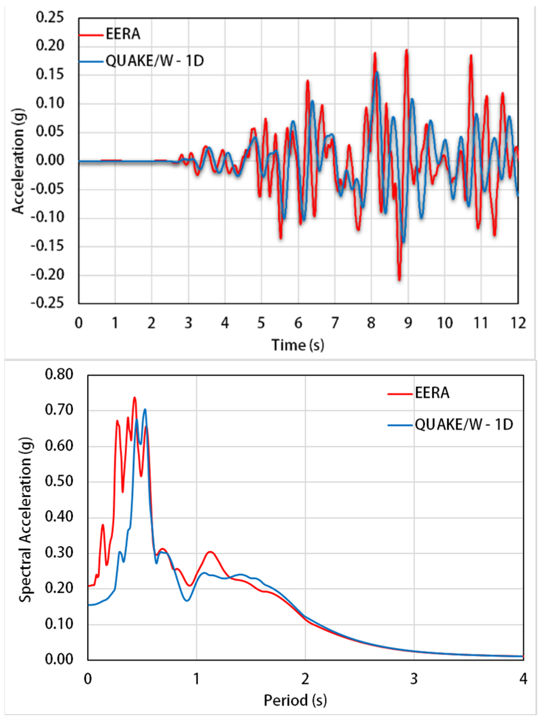
Figure 14.
Comparison between 1-D analyses performed by EERA and QUAKE/W for point 2, in terms of acceleration time history and spectral acceleration, for the Amoruso et al. [26] input.
Figure 14.
Comparison between 1-D analyses performed by EERA and QUAKE/W for point 2, in terms of acceleration time history and spectral acceleration, for the Amoruso et al. [26] input.

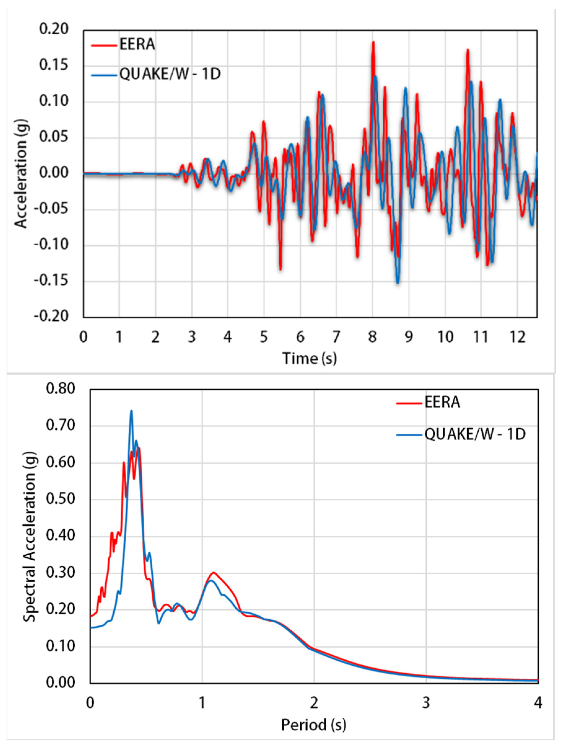
Figure 15.
Comparison between 1-D analyses performed by EERA and QUAKE/W for point 3, in terms of acceleration time history and spectral acceleration, for the Amoruso et al. [26] input.
Figure 15.
Comparison between 1-D analyses performed by EERA and QUAKE/W for point 3, in terms of acceleration time history and spectral acceleration, for the Amoruso et al. [26] input.

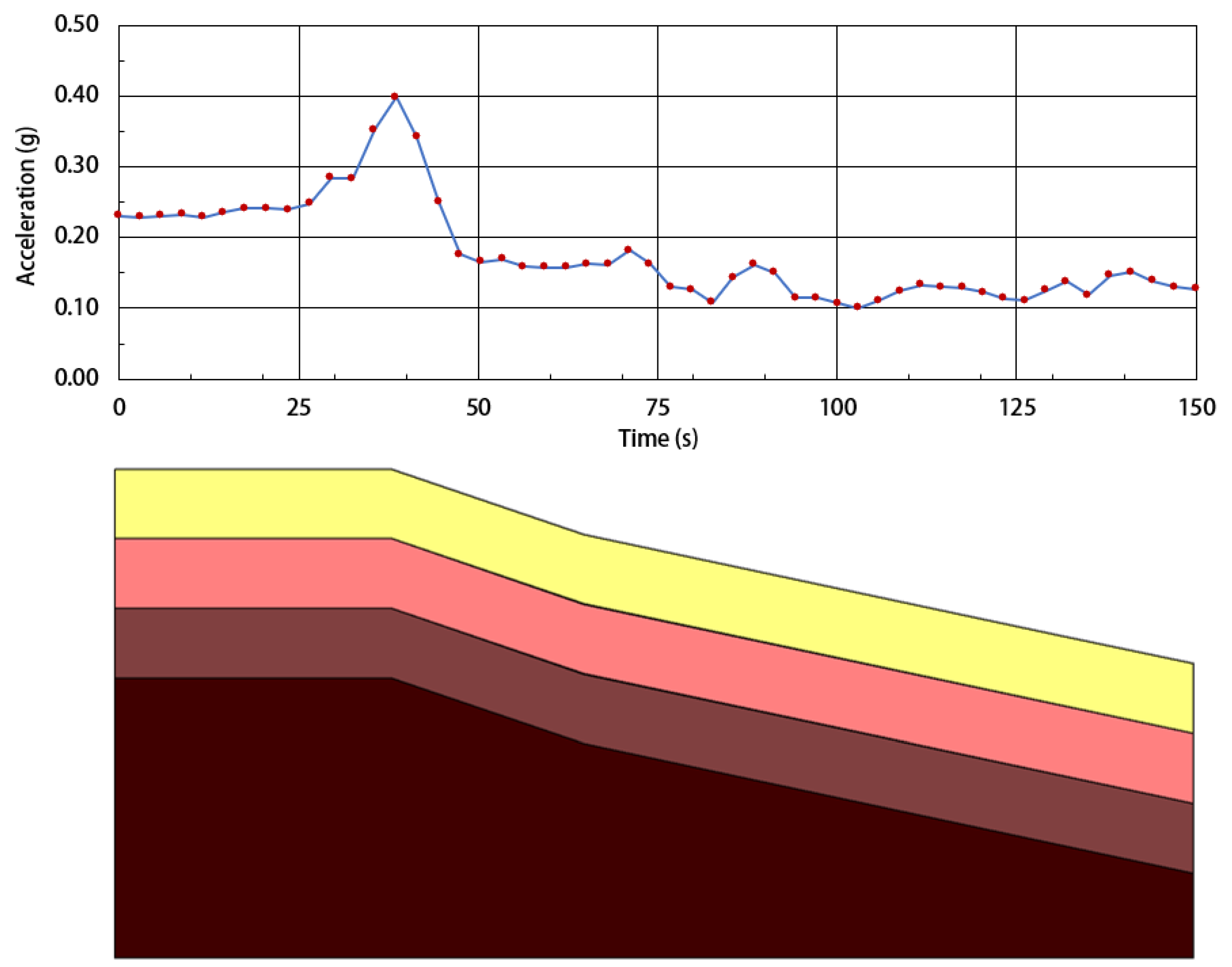
Figure 16.
Surface acceleration profile along the 2-D section analyzed through QUAKE/W code for the Amoruso et al. [26] input.
Figure 16.
Surface acceleration profile along the 2-D section analyzed through QUAKE/W code for the Amoruso et al. [26] input.

Figure 17.
Comparison between 1-D and 2-D analyses performed by EERA and QUAKE/W for point 1 in terms of acceleration time history and spectral acceleration, for the Amoruso et al. [26] input.
Figure 17.
Comparison between 1-D and 2-D analyses performed by EERA and QUAKE/W for point 1 in terms of acceleration time history and spectral acceleration, for the Amoruso et al. [26] input.

Figure 18.
Comparison between 1-D and 2-D analyses performed by EERA and QUAKE/W for point 2 in terms of acceleration time history and spectral acceleration, for the Amoruso et al. [26] input.
Figure 18.
Comparison between 1-D and 2-D analyses performed by EERA and QUAKE/W for point 2 in terms of acceleration time history and spectral acceleration, for the Amoruso et al. [26] input.

Figure 19.
Comparison between 1-D and 2-D analyses performed by EERA and QUAKE/W for point 3 in terms of acceleration time history and spectral acceleration, for the Amoruso et al. [26] input.
Figure 19.
Comparison between 1-D and 2-D analyses performed by EERA and QUAKE/W for point 3 in terms of acceleration time history and spectral acceleration, for the Amoruso et al. [26] input.

Figure 20.
Ashford and Sitar’s [46] model for the topographical amplification evaluation.
Figure 20.
Ashford and Sitar’s [46] model for the topographical amplification evaluation.

Figure 21.
Topographic Aggravation Factor (TAF), after the Kallou et al. [48] approach, obtained as the ratio of the Fourier amplitude spectra at the crest and behind the crest, for the Amoruso et al. [26] input.

Figure 22.
Topographic Aggravation Factor (TAF), after the Bouckovalas and Kouretzis [49] approach, in terms of (2-D)/(l-D) ratio of elastic response spectra obtained at the crest, for the Amoruso et al. [26] input.

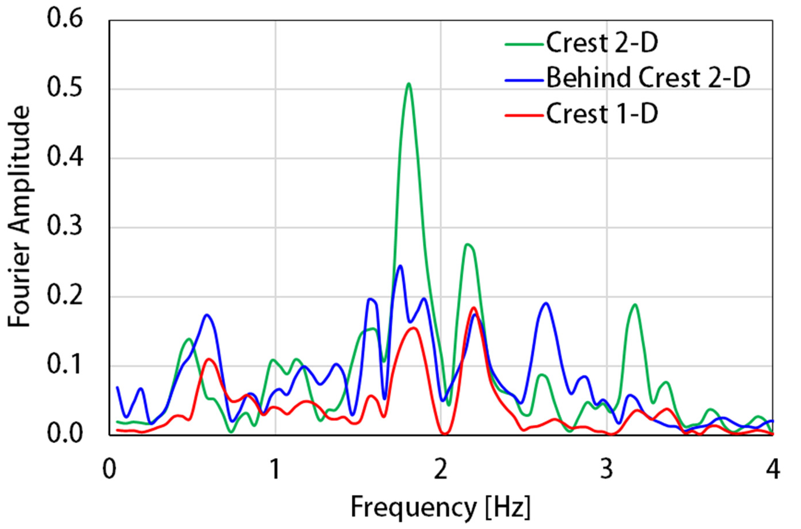
Figure 23.
Comparison between Fourier amplitude spectra at the crest (1-D and 2-D) and behind the crest (2-D), for the Amoruso et al. [26] input.
Figure 23.
Comparison between Fourier amplitude spectra at the crest (1-D and 2-D) and behind the crest (2-D), for the Amoruso et al. [26] input.

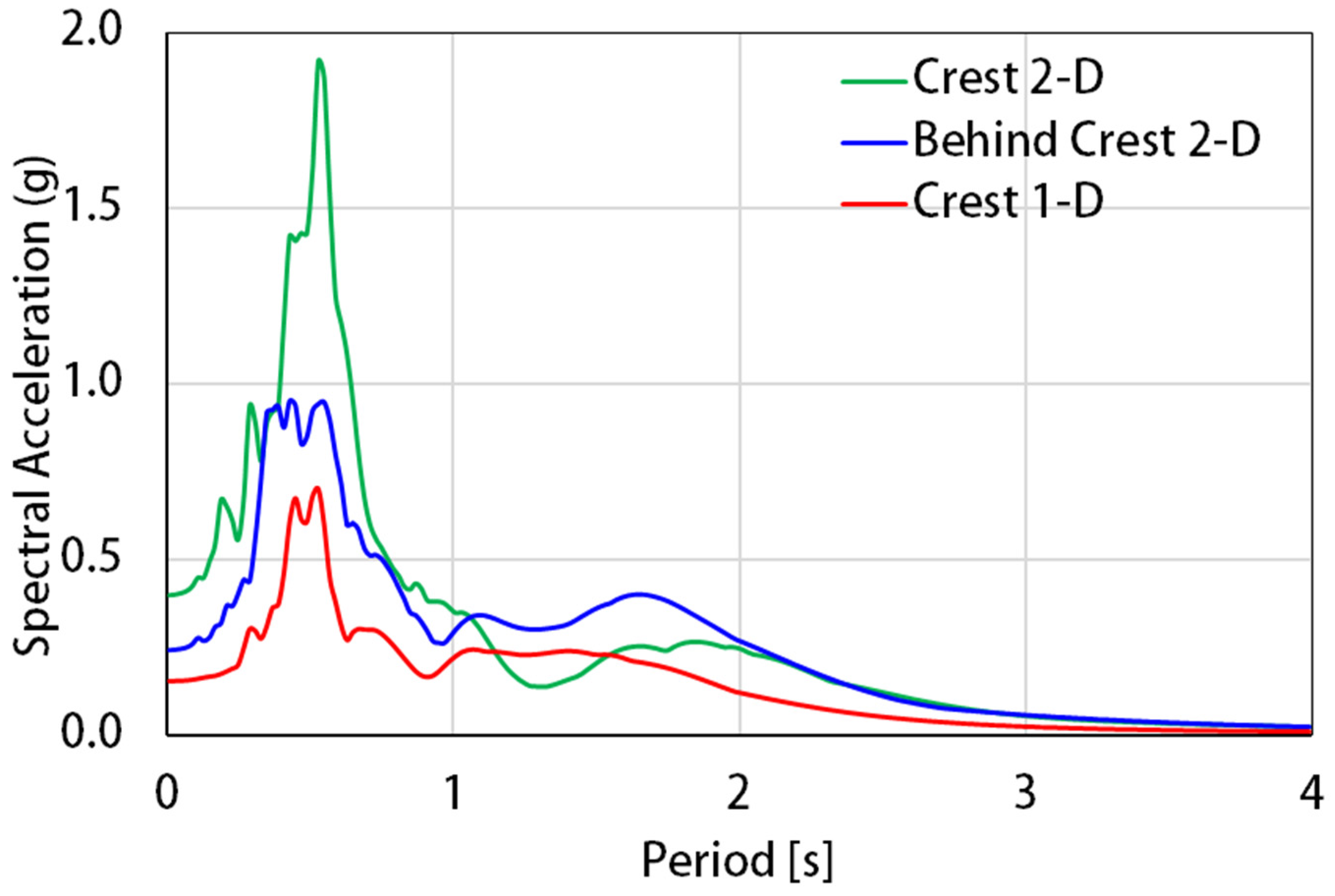
Figure 24.
Comparison between elastic response spectra at the crest (1-D and 2-D) and behind the crest (2-D), for the Amoruso et al. [26] input.
Figure 24.
Comparison between elastic response spectra at the crest (1-D and 2-D) and behind the crest (2-D), for the Amoruso et al. [26] input.


Table 1.
Soil profile for Caronia area.
| Borehole | D [m] | Soil Profile | VS [m/s] |
|---|---|---|---|
| BH105 | 0.00–4.00 | Debris: conglomerate screed, boulders and chaotic material. | <260 |
| BH105 | 4.00–15.50 | Tobacco brown clays, to the touch plastic and from medium consistent to consistent in the lower part (10.50–15.50 m); at times there are clay levels; overall, when cut, they present themselves with ferrous, rust-colored and alternatively gray alterations. | <350 |
| BH105 | 15.50–31.00 | Dark gray clay with very consistent sections, alternating with fractured and flattened layers; moreover, there are rare levels of clay with plastic behavior and dark color. | >450 <600 |
| BH3 | 0.00–4.00 | Plastic structureless clays (landslide debris). | <260 |
| BH3 | 4.00–6.00 | Chaotic structureless clay with occasional compact clay levels of brown color with plastic consistency and poor characteristics. | <350 |
| BH3 | 6.00–15.50 | Chaotic structureless clay with occasional compact clay levels of gray color with plastic consistency and mediocre characteristics. | >350 <450 |
| BH3 | 15.50–31.00 | Argillites with lytic tracts and sub-vertical fractures, dark gray or blackish in color with mediocre characteristics. | >450 <600 |
where: D = Depth, VS = Shear Wave Velocity and BH105 or BH3 = Boreholes where the profiles were taken.
Table 2.
Mechanical characteristics for Caronia area.
| Site | D [m] | γ [kN/m3] | Wn [%] | WL [%] | WP [%] | PI [%] | CI [%] | AI [%] |
|---|---|---|---|---|---|---|---|---|
| BH2CI1 | 2.50–3.00 | 19.81 | 12.54 | 34.17 | 11.98 | 22.19 | 0.97 | 1.07 |
| BH3CI1 | 2.50–3.00 | 19.71 | 26.21 | 31.78 | 22.71 | 9.07 | 1.58 | 0.34 |
| BH3CI2 | 6.00–6.40 | 19.61 | 22.65 | 37.63 | 19.74 | 17.89 | 0.97 | 0.44 |
| BH4CI1 | 7.30–7.60 | 18.24 | 15.78 | 53.27 | 20.20 | 33.07 | 0.99 | 0.64 |
| BH4CI2 | 10.70–11.00 | 19.22 | 24.45 | 22.58 | 13.42 | 9.16 | 1.29 | 0.52 |
| BH5CI1 | 12.00–12.45 | 19.12 | 26.35 | 48.56 | 20.06 | 28.50 | 0.96 | 0.48 |
| BH102-CM1 | 4.20–450 | 19.71 | 14.12 | 38.00 | 17.00 | 21.00 | 1.14 | 0.87 |
| BH2CI1 | 2.50–3.00 | 19.81 | 12.54 | 34.17 | 11.98 | 22.19 | 0.97 | 1.07 |
| BH3CI1 | 2.50–3.00 | 19.71 | 26.21 | 31.78 | 22.71 | 9.07 | 1.58 | 0.34 |
| BH3CI2 | 6.00–6.40 | 19.61 | 22.65 | 37.63 | 19.74 | 17.89 | 0.97 | 0.44 |
| BH4CI1 | 7.30–7.60 | 18.24 | 15.78 | 53.27 | 20.20 | 33.07 | 0.99 | 0.64 |
| BH4CI2 | 10.70–11.00 | 19.22 | 24.45 | 22.58 | 13.42 | 9.16 | 1.29 | 0.52 |
where: D = Depth, γ = Total Unit Weight, Wn = Water Content, WL = Liquid Limit, WP = Plastic Limit, PI = Plasticity Index, CI = Consistence Index and AI = Activity Index.
Table 3.
Mechanical characteristics for Caronia area.
| Site | D [m] | e | n | Sr [%] | c’ [kPa] | φ‘ [°] |
|---|---|---|---|---|---|---|
| BH2CI1 | 2.50–3.00 | 0.51 | 0.34 | 66.58 | 4.88 | 31.6 |
| BH3CI1 | 2.50–3.00 | 0.66 | 0.40 | 69.89 | 5.86 | 27.6 |
| BH3CI2 | 6.00–6.40 | 0.66 | 0.40 | 81.96 | 6.93 | 23.4 |
| BH4CI1 | 7.30–7.60 | 0.57 | 0.36 | 95.58 | 19.95 | 28.1 |
| BH4CI2 | 10.70–11.00 | 0.43 | 0.30 | 67.06 | 21.73 | 15.8 |
| BH5CI1 | 12.00–12.45 | 0.74 | 0.43 | 78.96 | 2.41 | 16.0 |
| BH102-CM1 | 4.20–450 | 0.52 | 0.34 | 73.12 | 33.20 | 21 |
| BH2CI1 | 2.50–3.00 | 0.44 | 0.30 | 67.02 | 20.30 | 22 |
| BH3CI1 | 2.50–3.00 | 0.49 | 0.33 | 78.88 | 36.50 | 30 |
| BH3CI2 | 6.00–6.40 | 0.44 | 0.31 | 85.07 | 51.80 | 22 |
| BH4CI1 | 7.30–7.60 | 0.39 | 0.28 | 73.30 | 34.00 | 20 |
| BH4CI2 | 10.70–11.00 | 0.35 | 0.26 | 85.63 | 23.20 | 21 |
where: D = Depth, e = Void Ratio, n = Porosity, Sr = Degree of Saturation, c’ = Cohesion and φ‘ = Effective friction angle from Direct Shear Test (DST).
Table 4.
Soil constants for Caronia area.
| Soil | α | β | η | λ |
|---|---|---|---|---|
| Debris | 65 | 1.15 | 34.8 | 1.9 |
| Brown Clay | 20 | 0.87 | 19 | 2.3 |
| Dark Gray Clay | 7.5 | 0.897 | 90 | 4.5 |
Table 5.
PGA (Peak Ground Acceleration) by 1-D analyses for the Amoruso et al. [26] input at point 1, 2 and 3.
Table 5.
PGA (Peak Ground Acceleration) by 1-D analyses for the Amoruso et al. [26] input at point 1, 2 and 3.
| PGAEERA [g] | PGAQUAKE/W 1-D [g] | |
|---|---|---|
| Point 1 | 0.228 | 0.207 |
| Point 2 | 0.228 | 0.207 |
| Point 3 | 0.168 | 0.141 |
Table 6.
PGA by 1-D analyses for the Bottari et al. [24], Tortorici et al. [25], DISS Messina Strait, DISS Gioia Tauro, DISS Aspromonte Est, 1693 Catania earthquake inputs at point 1, 2 and 3.
| Tortorici et al. [25] | Bottari et al. [24] | DISS Messina Strait | ||||
|---|---|---|---|---|---|---|
| PGA EERA | PGA QUAKE/W 1-D | PGA EERA | PGA QUAKE/W 1-D | PGA EERA | PGA QUAKE/W 1-D | |
| [g] | [g] | [g] | [g] | [g] | [g] | |
| Point 1 | 0.208 | 0.193 | 0.208 | 0.156 | 0.195 | 0.269 |
| Point 2 | 0.208 | 0.193 | 0.208 | 0.156 | 0.195 | 0.269 |
| Point 3 | 0.176 | 0.147 | 0.184 | 0.152 | 0.165 | 0.151 |
| DISS Gioia Tauro | DISS Aspromonte Est | 1693 Catania Earthquake | ||||
| PGA EERA | PGA QUAKE/W 1-D | PGA EERA | PGA QUAKE/W 1-D | PGA EERA | PGA QUAKE/W 1-D | |
| [g] | [g] | [g] | [g] | [g] | [g] | |
| Point 1 | 0.257 | 0.203 | 0.206 | 0.266 | 0.179 | 0.142 |
| Point 2 | 0.257 | 0.203 | 0.206 | 0.266 | 0.179 | 0.142 |
| Point 3 | 0.202 | 0.157 | 0.181 | 0.167 | 0.154 | 0.117 |
Table 7.
PGA by 1-D and 2-D analyses for the Amoruso et al. [26] input at point 1, 2 and 3.
Table 7.
PGA by 1-D and 2-D analyses for the Amoruso et al. [26] input at point 1, 2 and 3.
| PGAEERA [g] | PGAQUAKE/W 1-D [g] | PGAQUAKE/W 2-D [g] | |
|---|---|---|---|
| Point 1 | 0.208 | 0.156 | 0.242 |
| Point 2 | 0.208 | 0.156 | 0.400 |
| Point 3 | 0.184 | 0.152 | 0.138 |
Table 8.
PGA by 1-D and 2-D analyses for the Tortorici et al. [25], Bottari et al. [24], DISS Messina Strait, DISS Gioia Tauro, DISS Aspromonte Est, 1693 Catania earthquake inputs at point 1, 2 and 3.
| Tortorici et al. [25] | Bottari et al. [24] | DISS Messina Strait | |||||||
|---|---|---|---|---|---|---|---|---|---|
| PGA EERA | PGA QUAKE/W 1-D | PGA QUAKE/W 2-D | PGA EERA | PGA QUAKE/W 1-D | PGA QUAKE/W 2-D | PGA EERA | PGA QUAKE/W 1-D | PGA QUAKE/W 2-D | |
| [g] | [g] | [g] | [g] | [g] | [g] | [g] | [g] | [g] | |
| Point 1 | 0.208 | 0.193 | 0.311 | 0.228 | 0.207 | 0.336 | 0.195 | 0.269 | 0.403 |
| Point 2 | 0.208 | 0.193 | 0.400 | 0.228 | 0.207 | 0.370 | 0.195 | 0.269 | 0.493 |
| Point 3 | 0.176 | 0.147 | 0.083 | 0.168 | 0.141 | 0.064 | 0.165 | 0.151 | 0.140 |
| DISS Gioia Tauro | DISS Aspromonte Est | 1693 Catania Earthquake | |||||||
| PGA EERA | PGA QUAKE/W 1-D | PGA QUAKE/W 2-D | PGA EERA | PGA QUAKE/W 1-D | PGA QUAKE/W 2-D | PGA EERA | PGA QUAKE/W 1-D | PGA QUAKE/W 2-D | |
| [g] | [g] | [g] | [g] | [g] | [g] | [g] | [g] | [g] | |
| Point 1 | 0.257 | 0.203 | 0.369 | 0.206 | 0.266 | 0.493 | 0.179 | 0.142 | 0.121 |
| Point 2 | 0.257 | 0.203 | 0.373 | 0.206 | 0.266 | 0.536 | 0.179 | 0.142 | 0.140 |
| Point 3 | 0.202 | 0.157 | 0.197 | 0.181 | 0.167 | 0.156 | 0.154 | 0.117 | 0.054 |
Table 9.
Different results for the Ashford et al. [47] model.
Publisher’s Note: MDPI stays neutral with regard to jurisdictional claims in published maps and institutional affiliations. |
© 2021 by the authors. Licensee MDPI, Basel, Switzerland. This article is an open access article distributed under the terms and conditions of the Creative Commons Attribution (CC BY) license (https://creativecommons.org/licenses/by/4.0/).
Share and Cite
MDPI and ACS Style
Cavallaro, A.; Ferraro, A.; Grasso, S.; Puccia, A. 2-D Seismic Response Analysis of a Slope in the Tyrrhenian Area (Italy). Appl. Sci. 2021, 11, 3180. https://0-doi-org.brum.beds.ac.uk/10.3390/app11073180
AMA Style
Cavallaro A, Ferraro A, Grasso S, Puccia A. 2-D Seismic Response Analysis of a Slope in the Tyrrhenian Area (Italy). Applied Sciences. 2021; 11(7):3180. https://0-doi-org.brum.beds.ac.uk/10.3390/app11073180
Chicago/Turabian StyleCavallaro, Antonio, Antonio Ferraro, Salvatore Grasso, and Antonio Puccia. 2021. "2-D Seismic Response Analysis of a Slope in the Tyrrhenian Area (Italy)" Applied Sciences 11, no. 7: 3180. https://0-doi-org.brum.beds.ac.uk/10.3390/app11073180
Note that from the first issue of 2016, this journal uses article numbers instead of page numbers. See further details here.