Article

Data Assimilation of AOD and Estimation of Surface Particulate Matters over the Arctic

1
School of Earth Sciences and Environmental Engineering, Gwangju Institute of Science and Technology (GIST), Gwangju 61005, Korea
2
Center for Earth Environmental Modeling Studies (CEMOS), Gwangju Institute of Science and Technology (GIST), Gwangju 61005, Korea
3
Department of Health Management, Kyung-in Women’s University, Incheon 21041, Korea
4
Korea Institute of Atmospheric Prediction System, Seoul 07071, Korea
5
Department of Safety and Environment Research, The Seoul Institute, Seoul 06756, Korea
6
Institute for Atmospheric and Earth System Research/ Physics, Faculty of Science, University of Helsinki, 00014 Helsinki, Finland
7
Department of Magnetism, Institute of Geophysics, Polish Academy of Sciences, Księcia Janusza St. 64, 01-452 Warsaw, Poland
8
Department of Physics of The Atmosphere, Institute of Geophysics Polish Academy of Sciences, Księcia Janusza St. 64, 01-452 Warsaw, Poland
9
Korea Polar Research Institute (KOPRI), Incheon 21990, Korea
*
Author to whom correspondence should be addressed.
Submission received: 4 January 2021 / Revised: 15 February 2021 / Accepted: 18 February 2021 / Published: 23 February 2021
(This article belongs to the Special Issue Air Pollution II)

Abstract

:
In this study, more accurate information on the levels of aerosol optical depth (AOD) was calculated from the assimilation of the modeled AOD based on the optimal interpolation method. Additionally, more realistic levels of surface particulate matters over the Arctic were estimated using the assimilated AOD based on the linear relationship between the particulate matters and AODs. In comparison to the MODIS observation, the assimilated AOD was much improved compared with the modeled AOD (e.g., increase in correlation coefficients from −0.15–0.26 to 0.17–0.76 over the Arctic). The newly inferred monthly averages of PM10 and PM2.5 for April–September 2008 were 2.18–3.70 μg m−3 and 0.85–1.68 μg m−3 over the Arctic, respectively. These corresponded to an increase of 140–180%, compared with the modeled PMs. In comparison to in-situ observation, the inferred PMs showed better performances than those from the simulations, particularly at Hyytiala station. Therefore, combining the model simulation and data assimilation provided more accurate concentrations of AOD, PM10, and PM2.5 than those only calculated from the model simulations.

1. Introduction

The Arctic haze composed of sulfate, black carbon, organic matter transported from the mid-latitude industrial regions of Europe, Russia, and Asia has influences on perturbation of the radiation balance between the surface and the top-of-atmosphere over the Arctic [1,2,3,4,5,6]. First, the transported haze particles warm or cool the atmosphere by scattering or absorbing sunlight, which is the direct effect of aerosol [6,7]. Second, it interacts with clouds to produce more and smaller droplets, leading to more warmth, which are indirect effects of aerosol [8,9,10]. Third, when haze particles deposit into the snow or ice, they absorb more sunlight by reducing the surface albedo [11].
Many observations for gaseous species, particulate matters, and clouds have been carried out at several stations of Ny-Ålesund (Svalbard), Pallas-Sodankylä (Finland), Villum (Greenland), Summit (Greenland), Alert (Canada), Eureka (Canada), Oliktok Point (USA), Barrow (USA), Cherskii (Russia), Tiksi (Russia), Thule (Greenland), Hornsund (Svalbard), and Andenes (Norway) over the Arctic regions to examine the global climate changes, air pollution, and their interaction [12,13,14,15,16,17,18]. Since these observations were spatially sparse, there was a spatial limitation in providing detailed atmospheric information over the Arctic. However, it is hard to measure a variety of chemical/physical parameters and species in three dimensions at the same time. Additionally, in the Arctic regions, there are many restrictions on research activities due to extreme weather conditions. Nevertheless, there have been observational efforts to obtain three-dimensional and various information. The intensive field campaigns, including aircraft-based observation, have been conducted temporarily in a limited way for several weeks in spring and summer under good weather, as follows: (i) Arctic Study of Tropospheric Aerosol, Clouds and Radiation (ASTAR) [19], (ii) Aerosol, Radiation, and Cloud Processes affecting Arctic Climate (ARCPAC) [20], (iii) Arctic Research of Composition of the Troposphere from Aircraft and Satellite-Phase A and B (ARCTAS-A and B) [21,22], and (iv) POLARCAT-Greenland Aerosol and Chemistry Experiment (POLARCAT-GRACE) [23] campaigns during the International Polar Year (IPY) in 2007 and 2008.
Satellite observation and model simulation are alternatives for large and extreme environmental regions such as the Arctic [24]. However, these tools also have the following advantages and limitations. Although satellite-observed data is relatively more accurate than the model simulation, there are also limitations in spatial and temporal information. While the model simulation provides perfect spatial information for all atmospheric variables on an hourly basis, the accuracy of the simulated data is relatively low due to the uncertainties related to emissions, boundary conditions, and parameterization for aerosol calculation and atmospheric chemistry [25,26]. In particular, since the atmospheric levels of PMs are known to be low over the Arctic, the uncertainty in (ship) emissions and information on pollutants transported from Europe, Russia, and Asia strongly links with the performance of model simulation in the Arctic. To solve the issue, many efforts have been made to conduct the data assimilation of PMs and AOD based on the variational approach (e.g., 3DVAR and 4DVAR) [27,28,29,30,31,32,33,34,35], sequential approach (e.g., optimal interpolation, Ensemble Kalman Filter) [36,37,38,39,40,41,42,43,44,45,46,47,48,49], and the combined method [50,51]. For example, Liu et al. developed the National Centers for Environmental Prediction (NCEP) Gridpoint Statistical Interpolation (GSI) three-dimensional variational (3DVAR) data assimilation system applied to a dust storm in East Asia [30]. Chai et al. showed promising results in better estimation in the PM2.5 concentration using the data assimilation of the MODIS-observed AOD with optimal interpolation (OI) method in the US [47]. Therefore, in this study, we also attempted to overcome the spatial and temporal limitations in the satellite observation and the low accuracy in the model simulation through the data assimilation based on the OI method.
The objective of the study is to estimate realistic levels of surface particulate matter over the Arctic. For this purpose, more accurate AODs are calculated via the data assimilation procedure using the satellite and ground remotely sensed data.

2. Experiments

2.1. Description of WRF/CMAQ Model Simulations

A year-long Chemistry Transport Model (CTM) simulation was carried out to understand the levels of particulate matter over the Arctic. WRF v3.4.1 modeling [52] was also carried out to generate meteorological fields, acting as drivers and/or driving atmospheric chemical and physical processes of the regional CTM model, such as (i) the transports of species; (ii) chemical losses through chemical reactions and photolysis; (iii) physical removal through dry and wet depositions. For the WRF model simulation, the initial and lateral boundary conditions were taken from the National Center for Environmental Prediction (NCEP) data [53,54]. The WRF simulation was configured with the following physical options shown in Table 1.
As a 3D-CTM, Community Multi-scale Air Quality (CMAQ) v5.1 model was employed to simulate the levels of air pollutants over the Arctic for the year 2008 [61]. We decided on 2008 as the target year because many modeling and observation studies were conducted as part of POLARCAT-IPY, aiming at improving understanding of Arctic pollution and its impact on climate during International Polar Year (IPY) in 2007 and 2008 [62]. From a meteorological perspective, it is unusual for the Arctic weather in 2008, which showed an abnormally cold winter in Greenland, especially with an intense melt season [63]. The modeling domain centered on Svalbard was configured with 18 km × 18 km horizontal grid spacing and vertical resolution of 17 layers from surface to 80 hPa, covering the Arctic Ocean, Greenland Sea, Barents Sea, Norwegian Sea, Greenland, Queen Elizabeth Island, and some parts of Norway, Sweden, Finland, and Russia (Figure 1a). We employed the SAPRC-07 mechanism and AERO6 module for the gas-phase chemistry and aerosol (thermo) dynamics, respectively (Table 1). Information on boundary conditions for atmospheric gases and aerosols were taken from the output simulated by the Model for Ozone and Related Chemical Tracers, version 4 (MOZART-4) model (http://www.acom.ucar.edu/wrf-chem/mozart.shtml) [64].
The anthropogenic emissions of gaseous and particulate species were obtained from the Monitoring Atmospheric Composition and Climate and megacity Zoom for the Environment projects (MACCity), which has a 0.5° resolved database compiled for the year 2008 [65]. For PM10 and PM2.5, the anthropogenic emissions were taken into account from the Evaluating the Climate and Air Quality Impacts of Short-lived Pollutants (ECLIPSE) v4a emission inventories based on the CLE scenario [66]. Furthermore, to consider biogenic and biomass burning emissions, we used the 0.5° resolved Model of Emissions of Gases and Aerosols from Nature-Monitoring Atmospheric Composition and Climate (MEGAN-MACC) and Global Fire Emissions Database v3 (GFED3) emission inventories, respectively [67,68]. All emissions were downloaded from the ECCAD archive (https://eccad3.sedoo.fr/). Figure 1 presented the annual emission fluxes of SO2, NOx, EC, OC, PM10, and PM2.5 used in the CMAQ model simulations. High emission fluxes were found over Finland and Russia in the study domain. Despite relatively fewer amounts of emissions, the ship-emitted pollutants were considered in the emission inventory. The emissions can be seen along the coastal lines of Norway and Iceland.

2.2. Description of Remote-Sensed Observations

The mission of the MODIS instrument equipped on the NASA Earth Observation System (EOS) platforms of Terra and Aqua satellites is to capture the vertical columnar aerosol loading and aerosol properties such as AOD, Angström exponent, and single scattering albedo over the cloud- and snow-free land and ocean. The MODIS/Terra observes the atmosphere with a descending orbit, passing over the equator at about 10:30 local sun time while the MODIS/Aqua flies northward across the equator at about 13:30 local sun time. In particular, the vertically-integrated aerosol extinction (i.e., AOD, τMODIS) observed by the MODIS sensor has been used to evaluate the performance of 3D-CTM and conduct the data assimilation of the model-calculated AODs [69,70,71]. For such purpose of study, we obtained the daily level 2 AOD of Terra satellite (MOD04_L2) from the NASA LAADS (https://ladsweb.modaps.eosdis.nasa.gov/search/). The AOD products were retrieved at a wavelength of 550 nm through the NASA Collection 6 algorithm (C6). Although, latest product via the C6.1 algorithm were released, there is no change in the combined dataset between the C6 and C6.1 collections [72].
The C6 includes three retrieval algorithms, which are (i) Dark Target (DT) over vegetated/dark-soiled land retrieved in the visible wavelength [73,74], (ii) Deep Blue (DB) over the brighter surface in the visible wavelength (e.g., deserts) [75], and (iii) DT over water surface in the visible and longer wavelength [74,76]. The expected uncertainty of AOD was reported to be ± (0.05 ± 15%) over land and (0.04 ± 10%, −0.02 ± 10%) over the ocean [74]. Levy et al. also reported that in comparison with AERONET-retrieved AODs (τAERONET), 69.4% of τMODIS fall within expected error [74]. In this study, to use more gap-filled data set, we used a merged AOD product combining the DT with DB over ocean and land, which is “AOD_550_Dark_Target_Deep_Blue_Combined” data with a spatial resolution of 10 km × 10 km at the nadir (and 48 km × 20 km near the swath edge) and the temporal resolution of 5 min [74,77]. In the analysis, only pixels recommended quality assurance, good and very good flag (QA = 2 and 3) were used [77]. The MODIS-retrieved AOD (τMODIS) were re-gridded to a model grid of 18 km × 18 km on a daily basis.
Figure S1 shows a spatiotemporal map of the monthly availability of data for the entire domain, using the merged AOD product. As expected, there were large numbers of missing pixels over the Arctic Ocean and Greenland because of high surface albedo due to sea ice and snow cover. The low data availability over the Arctic Ocean region greatly varies from season to season. On the other hand, higher than 30% of data availability was found frequently over some parts of the Greenland Sea, Barents Sea, and the Norwegian Sea. The results indicate that data integration (or assimilation) between model-calculated and satellite-observed AODs is needed for the regions showing high surface albedo such as the Arctic to address the defects of each model estimation and satellite observation and to maximize their advantages.
The AOD product retrieved from the C6 algorithm has been validated with the AERONET-observed AOD (τAERONET), which is a global network of ground-based sun/sky-photometers [78]. The sun-photometers measures the sun radiances at the eight typical channels of 340, 380, 440, 500, 675, 870, 1020, and 1640 nm. The sun-photometers-measured AODs are regarded as truth because the ground observations are not affected by surface reflectivity. Thus, in the study, we employed the available AERONET AOD data at five monitoring sites (Hornsund, Thule, Andenes, Kuopio, and Hyytiala stations) to evaluate the CMAQ-calculated, MODIS-retrieved, and assimilated-AODs over the Arctic. As shown in Figure 1a, the Thule, Hornsund, and Andenes stations are adjacent to the coast, so the AODs in the areas is easily affected by sea salt particles. On the other hand, the Kuopio and Hyytiala stations are located in the inner parts of Finland, which the air quality is affected by anthropogenic sources. The level 2.0 product of AOD obtained from the AERONET archive (https://aeronet.gsfc.nasa.gov) is cloud-screened, quality-controlled, processed via version 3.0 algorithm [79]. Here, AOD at 550 nm was selected as the same as τMODIS and calculated by Equations (1) and (2):
τ λ = τ λ 0 λ λ 0 α
where, λ and λ0 represent wavelengths at 550 nm and 500 nm, respectively. The Angström exponent (α) was calculated from the 870 nm (λ1) and 440 nm (λ2) channels [80].
α = L o g τ λ 1 τ λ 2 L o g λ 1 λ 2
Figure 2 showed the seasonal scatter plots and statistical analysis between τAERONET and τMODIS over the 5 AERONET stations. For synchronization with the AERONET observation, the MODIS data were collected within at most 10 km and 30 min in the spatial and temporal differences.
As expected from Figure S1, the synchronized hourly dataset were small (N = 139 during the periods of April–September 2008) because the MODIS data-set was filtered due to the high surface albedo. The overall correlation coefficients (Index of Agreement) were 0.73 (0.81) and were good, particularly for April and August 2008. From the analysis, the slopes between τAERONET and τMODIS were smaller, in particular in warm seasons, which indicates that the MODIS AOD was possibly underestimated. Therefore, the underestimated τMODIS would affect the surface PM10 and PM2.5 estimations from the assimilated AOD. In the study, AERONET AODs (τAERONET) were also used to determine the free parameter for the data assimilation. The details were discussed later in Section 2.3.

2.3. CMAQ-Derived and Assimilated AODs

The radiant energy is attenuated in the atmosphere by aerosol scattering and absorption. The attenuation is expressed by the extinction coefficient (σext = σsct + σabs, unit: Mm−1), which depends on the particulate composition with respect to particle size [81]. With consideration of all modeled particulate species, the CMAQ-derived AOD was calculated by integrating the aerosol extinction coefficient vertically from the surface to the top-of-atmosphere:
τ C M A Q = i = 1 N σ s c t + σ a b s Δ z i = i = 1 N σ e x t Δ z i
where, Δzi and N are layer thickness at each layer and 17 layers, respectively. The AOD was calculated using the extinction coefficients estimated from the empirical “reconstructed mass-extinction method” as following Equations (4) and (5). We used the formula of Pitchford et al. [82] instead of the original Interagency Monitoring of PROtected Visual Environments (IMPROVE) extinction equation because of the possibly significant contributions of sea salt to extinction over the oceans [82,83]. Light scattering by sea salt aerosol was not considered in the original IMPROVE formula. Additionally, our domain covers a wide range of ocean, as shown in Figure 1.
σ e x t ( M m 1 ) s = 1 N α s , d r y f s ( R H ) [ C s ] 2.2 × f F ( R H ) × [ ( N H 4 ) 2 S O 4 ] F + 4.8 × f L ( R H ) × [ ( N H 4 ) 2 S O 4 ] L + 2.2 × f F ( R H ) × [ N H 4 N O 3 ] F + 4.8 × f L ( R H ) × [ N H 4 N O 3 ] L + 2.8 × [ O M ] F + 6.1 × [ O M ] L + 10.0 × [ E C ] F + 1.7 × f S S ( R H ) × [ S S ] + 0.6 × [ C O R S ] + 0.6 × [ S O I L ]
f F ( R H ) = f L ( R H ) = f S S ( R H ) = a 1 × R H 1 R H + a 2   for   R H b 1   f F ( R H ) = f L ( R H ) = f S S ( R H ) = 1   for   R H < b 1  
where, fs(RH) denotes the hygroscopic growth factor for ammonium sulfate, ammonium nitrate, and sea salt as a function of relative humidity (RH, %). Specifically, fs(RH) is classified into fF(RH), fL(RH), and fSS(RH) for fine, large, and sea salt particles, respectively. The fs(RH) is also function of coefficients of the a1 and a2 in Equation (5), which are 0.4175 and 1.2312 for fine aerosol (F), 0.2381 and 1.3276 for large aerosol (L), and 0.2913 and 2.3308 for sea salt (SS). The reference relative humidity (b1) is 37% for fine and coarse aerosol and 46% for sea salt. Cs represents the concentrations of species (s), which are organic mass (OM), element carbon (EC), sea salt (SS), coarse mass (CORS), and soil-derived mass (SOIL), respectively. αS,dry is the dry mass extinction coefficients (m2 g−1) of the species (s). Here, we used the constant values of αS,dry for ammonium sulfate, ammonium nitrate, sea salt, and organic mass calculated from the Mie theory at 550 nm under the dry condition [82].
Many investigators have used the data assimilation technique by combing modeling and observations to produce an optimal estimated AOD of the evolving state of the system [38,42,84]. We performed the data assimilation every hourly using the OI (optimal interpolation) method expressed as the following Equations (6)–(9). For the data assimilation, the MODIS data were collected every hour within a 30 min in time differences.
τ m = τ m + K ( τ 0 H τ m )
K = B H T ( H B H T + O ) 1
The τ’, τm, and τo represent hourly assimilated, model-calculated, and MODIS-observed AODs, respectively. H is the linear observation operator allowing the calculation of the model equivalents in observation location. K denotes the Kalman gain matrix combining the error covariance matrix for the modeled (B) and observed (O) fields.
O = ( f o τ o + ε o ) 2 Ι
B = ( f m τ m + ε m ) 2 exp d x 2 + d y 2 2 l x y 2
where, fo and fm represent fractional error coefficients in the observed and modeled τ, respectively. εo and εm are minimum error in the observed and modeled τ, respectively. dx and dy are horizontal grid resolution (i.e., dx = dy = 18 km in this study). lxy is the horizontal correlation length for errors in the modeled τ. In the sensitivity test, the best free parameters of fo, fm, εo, and εm on a monthly basis were determined by minimizing a statistical parameter of χ2 defined in Equation (10). This approach was introduced in the study of Park et al. [42]. The best values from the sensitivity test were summarized in Table S2.
χ 2 = 1 N i N ( τ i , A E R O N E T τ i , m ) 2 τ i , m
N is the number of available data set from the AERONET stations.

3. Results and Discussions

3.1. Simulated, Observed and Assimilated AODs over the Arctic

The CMAQ-calculated AOD (τCMAQ or τm) were compared to those from the MODIS observations (τMODIS or τo) to evaluate the performances of the model simulations over the Arctic. As shown in Figure 3 (i.e., green dots), the modeling performance was insufficient in terms of the correlation coefficients and slopes. There were almost no correlations between τCMAQ and τMODIS, showing the low values of −0.15–0.26 for all months. In addition, the slopes are under a bias towards the x-axis.
There are several uncertain issues of emission fluxes, chemistry transport model simulation, and AOD calculations. Among them, such large underestimations could be primarily related to the highly uncertain bottom-up emission fluxes over the Arctic. In Figure S2, we compared the emission fluxes of SO2, NOx, BC, OC, PM10, and PM2.5 from the several emission inventories over the regions (70° N–90° N; 60° W–60° E) including Greenland Sea, Barents Sea, and the Norwegian Sea. The most emissions over the areas can be attributed to the shipping activities. The oceanic regions were selected because the MODIS observed data were distributed mainly over the ocean due to high surface albedo over the Greenland and Arctic Ocean. As shown in Figure S2, the ECLIPSE inventory had the smallest values in their emission fluxes. Additionally, the emission fluxes were considerably different by emission inventory. The emission inventories (ECLIPSE and MACCity) used in the simulations were marked as an asterisk in Figure S2. For example, unlike the little amounts of PM10 for the ECLIPSE inventory, the emission fluxes were ~3 Gg yr−1 for both EDGARv4.2 and HTAPv2 and ~10 Gg yr–1 for EDGARv4.3.2. Such a comparison was also as similar as for PM2.5. For the species of BC and OC, the MACCity inventory showed relatively small emissions fluxes. In addition to anthropogenic sources, natural sea salt particles generated from the sea surface, particularly in coastal regions, have an enhanced contribution to the concentrations of particle matters over the ocean [85]. However, the estimations in the sea salt emissions are afflicted with several uncertain time-varying information on surf zone, wind speed, sea surface friction velocity, salinity, sea surface temperature, and dry sea salt particle size [86,87].
Figure 3 also shows the monthly scatter plots between the assimilated (τ’ or τAssim) and MODIS-retrieved AODs (τMODIS) and their statistical values over the entire domain (see the red dots). Compared to the statistical analyses between τCMAQ and τMODIS, those between τAssim and τMODIS was much improved. For example, the correlation coefficients were improved from −0.15–0.26 to 0.17–0.76. However, there were still low correlations, particularly in June and July. Additionally, the slopes between τAssim and τMODIS were close to 1:1 lines (S = 0.38–0.82), indicating the elevated AOD through the data assimilation. Such improvement can be visually seen from the spatial distributions of the τCMAQ, τMODIS, and τAssim in Figure S3.
The MODIS observed data produce a complete 2-dimensional set of AOD when assimilated into the CMAQ-calculated AOD. Thus, τAssim are much improved, compared with τCMAQ, particularly over Greenland Sea, Norwegian Sea, and the Barents Sea as shown in Figure S3. Nevertheless, τAssim was still underestimated compared to τMODIS. In the second column of Figure S3, the white pixels of τMODIS represent the areas indicating no available data due to cloud contamination or high surface reflectance.
Figure 4 showed the daily-mean variations of τAERONET, τMODIS, τCMAQ, and τAssim and their mean values at the AERONET stations of Thule, Hornsund, Andenes, Hyytiala, and Kuopio for 2008. In addition, the correlation coefficients among the AODs from AERONET, MODIS, CMAQ, and assimilation were calculated in Table 2 (see the bold numbers for the statically significant correlation coefficients in Table 2). In terms of daily variations, mean values, and statistical analysis, τAssim were improved, compared with τCMAQ.
The MODIS sensor similarly captures the levels of AODs observed by AERONET at all stations. The correlation coefficients between τMODIS and of τAERONET were from 0.52 to 0.91 (Table 2). The monthly similarity was also discussed in Figure 2. The similarity between τAERONET and τMODIS had a positive effect on the performance of data assimilation, which indicates that the accuracy of MODIS observations is primarily crucial in data assimilation. Thus, the AODs assimilated by the OI technique produced similar levels and daily-variations in AOD from the MODIS and AERONET observations, compared to the model-calculated AOD. Additionally, the analysis increments from the data assimilation system were still generated in some selected periods, although there were no sufficiently available data of MODIS AODs (e.g., τMODIS in March, April, and May at Hornsund station). The results are because the MODIS AODs observed in the adjacent areas provide a positive effect on the data assimilation. However, as shown in Figure 4, the effect of the data assimilation was insignificant since there were few available data of MODIS observation; in particular, in February, March, October, and November. Overall, from the analysis, we found that the combination between the CMAQ model and data assimilation based on OI method provided more accurate atmospheric levels and spatial distributions of AODs than those only calculated from the CMAQ simulations [88].

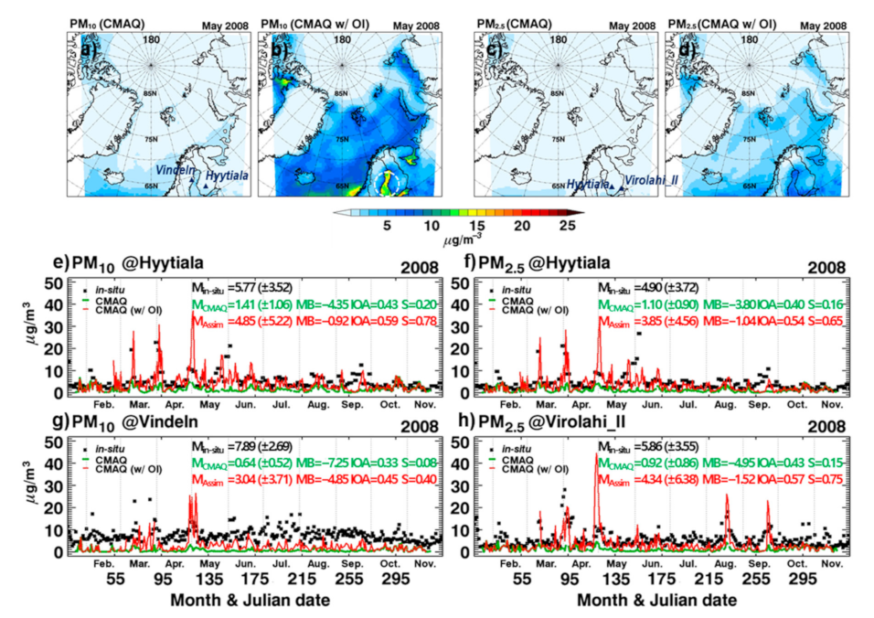
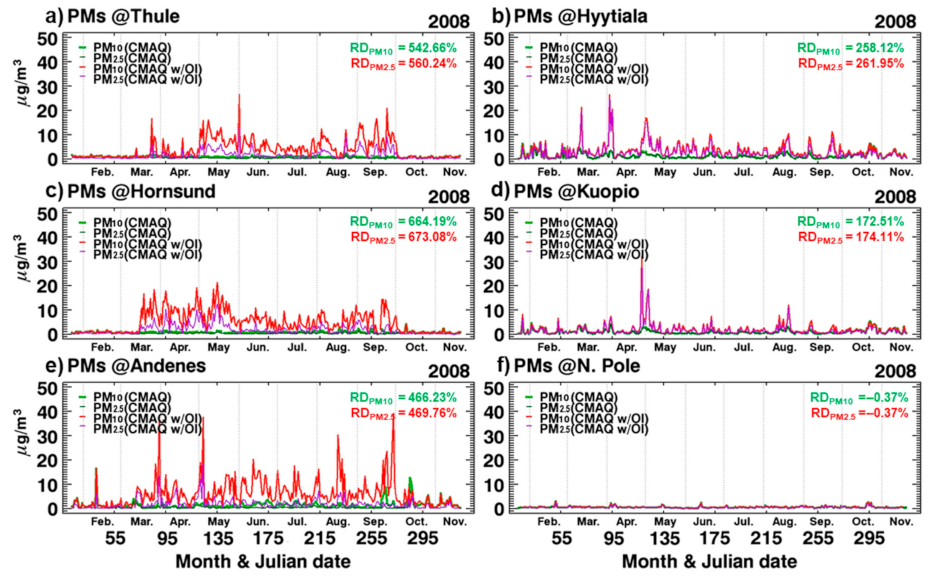
3.2. Estimations of Surface PMs from Assimilated AODs over the Arctic

Since the modeled AODs were highly underestimated (e.g., Figure 3 and Figure S3) due to the uncertain issues related to the emissions and boundary conditions, the low concentrations of PMs can be expected. Therefore, to estimate more realistic levels of PMs for the entire domain, the surface PMs were calculated using the assimilated AODs over the Arctic based on the linear relationship between the concentrations of PMs and AODs. For the estimations of PM10,CMAQ(w/OI) and PM2.5,CMAQ(w/OI), we used the Equations (11) and (12) because AOD is regarded as a proxy for concentrations of PMs in many studies [89,90].
P M 10 ,   C M A Q   ( w / O I ) = P M 10 ,   C M A Q τ C M A Q × τ C M A Q   ( w / O I )
P M 2.5 ,   C M A Q   ( w / O I ) = P M 2.5 ,   C M A Q τ C M A Q × τ C M A Q   ( w / O I )
Figure 5a–d and Figure S4 presented the spatial distributions of monthly averaged PM10 and PM2.5 concentrations calculated from the CMAQ simulations and inferred from the linear Equations (11) and (12). In Figure 5a,c, the concentrations of modeled PM10,CMAQ and PM2.5,CMAQ were smaller than 1–2 μg m−3 and were spatially homogeneous over the Arctic. In addition, it was clearly shown that the concentrations were relatively high in southern parts of the domain due to the influences of aerosols transported from the boundary. On the other hand, the concentrations of PM10 and PM2.5 inferred from the elevated AODs via data assimilation (shown in Figure 3 and Figure 4) increased by approximately 140–280% in April–September for the entire domain (refer to Table S1). Monthly average PM10,CMAQ(w/OI) and PM2.5,CMAQ(w/OI) inferred from the assimilated AODs were 3.50 (± 2.96) and 1.68 (± 1.38) μg m−3 over the entire domain in May, as shown in Figure 5b,d. We summarized the monthly mean of PM10 and PM2.5 for April–September in Table S1. Monthly means of PM10,CMAQ(w/OI) and PM2.5,CMAQ(w/OI) over the entire domain were between 2.18 and 3.70 μg m−3 and between 0.85 and 1.68 μg m−3, respectively. The maximum values of PM10,CMAQ(w/OI) and PM2.5,CMAQ(w/OI) were found along the coastline and over the Gulf of Bothnia, where the air quality is usually influenced by local air pollutants emitted from ships [91]. As shown in Figure 5b and Figure S3 for May, there can be a spatial inconsistency between the assimilated AOD and PMs,CMAQ(w/OI), particularly over the Gulf of Bothnia (i.e., white circle in Figure 5b. Such inconsistency is related to the vertical profile of aerosols because while the AODs are quantitative values of aerosols integrated from the surface to the top of the atmosphere, the PMs are the concentrations at the surface level.
For the validation, we compared the estimated PMs with in-situ observations. Figure 5e–h showed the daily mean variations of observed, simulated, and estimated PM10 and PM2.5 at Hyytiala, Vindeln, and Virolahi stations. While the temporal variations of the CMAQ-calculated PM10 and PM2.5 were almost flat, the inferred PMS,CMAQ(w/OI) well represented the high concentrations of observation. Compared to the in-situ observation (i.e., black squares), the PMS,CMAQ(w/OI) (i.e., red lines) inferred from the assimilation AODs showed better performance in the statistical point of view (see the M, MB, IOA, and S in the figure) than those from the CMAQ simulations (i.e., green lines), particularly at Hyytiala. The estimated average values of PM10,CMAQ(w/OI) were 4.85 and 3.04 μg m−3 at Hyytiala and Vindeln, respectively. Additionally, those of PM2.5,CMAQ(w/OI) were estimated to be 3.85 and 4.35 μg m−3 at Hyytiala and Virolahi, respectively. With low biases ranged from −1.52 to −0.92 μg m−3 except for Vindeln, these estimated values were close to the observations.
The temporal variations of PMS,CMAQ(w/OI) were also calculated at several sites of Thule, Hyytiala, Hornsund, Kuopio, Andenes, and the North Pole, as shown in Figure 6. The estimated surface concentrations of PM10,CMAQ(w/OI) (PM2.5,CMAQ(w/OI)) averaged for April–September were 5.88, 3.78, 6.37, 2.19, 7.99, 0.61 μg m−3 (2.21, 3.09, 2.54, 1.79, 2.25, 0.41 μg m−3), respectively. As shown in Figure 6, the estimated values increased by approximate 170–670% for all regions except the North Pole, compared to those from the CMAQ model simulations. The temporal variations of model-calculated PM10 and PM2.5 (colored as bright and dark green lines, respectively) remained flat. However, the estimated PM10,CMAQ(w/OI) and PM2.5,CMAQ(w/OI) (colored as red and purple lines, respectively) fluctuated considerably. In February, March, October, and November, the similar concentrations between the model-calculated PMS and the inferred PMS,CMAQ(w/OI) over Thule and Hornsund indicate that the effect of data assimilation is insignificant due to the absence of MODIS observed data originated from high surface reflectivity.
As shown in Figure 6, there were two separate groups divided in terms of the ratio of PM2.5 to PM10. The first group, having relatively low ratios, included Thule, Hornsund, and Andenes. Their ratios were 0.35, 0.35, and 0.30, respectively. These areas located near the coastal line have geographical conditions favorable for generating the coarse particle of sea salts. On the other hand, the second group, showing high ratios of PM2.5 to PM10 concentrations, were Hyytiala and Kuopio. The ratios were 0.80 and 0.77, respectively. These areas located in inland Finland are easily affected by anthropogenic sources. To confirm the origin of the air mass, we conducted the 5-day backward trajectory analysis for April–September using the HYSPLIT v5.0 [92]. From the trajectory analysis, we found that air masses at Hyytiala and Kuopio were mainly transported from Europe (39–47%) and the Arctic regions (38–46%) while those arriving at Thule, Hornsund, and Andenes were originated dominantly from the Arctic regions (81–92%).

4. Summaries and Conclusions

In the study, we examined the spatial and temporal variations of aerosol optical depths and estimated the surface PM10 and PM2.5 concentrations over the Arctic. For the investigation, a 1-year simulation was carried out over the Arctic using the WRF-CMAQ model. The performances of the WRF-CMAQ simulations were then evaluated by comparison with MODIS-observed AODs. The model-calculated AODs (τCMAQ) were highly underestimated, compared to the MODIS-retrieved AODs (τMODIS), and the correlation between τCMAQ and τMODIS was low over the Arctic.
To produce optimal estimated AODs, we utilized data assimilation based on the optimal interpolation (OI) technique by combing the model-calculated and satellite-observed AODs. The assimilated AODs (τAssim) were spatially and temporally compared with the MODIS and AERONET observed AODs. In terms of daily variations, mean values, and statistical analysis, τAssim were much more improved, compared with τCMAQ. The correlation coefficients were also improved from −0.15–0.26 to 0.17–0.76 over the Arctic. In the comparison with τMODIS, τAssim showed better correlation coefficients (R = 0.46–0.82) than those (R = 0.19–0.41) of τCMAQ at Thule, Hornsund, Andenes, and Hyytiala station. We also showed that the analysis increments from the data assimilation system were generated in some selected periods, although there were no sufficiently available data of MODIS AODs. Overall, combining the CMAQ model and satellite observation (based on the OI method) provided more accurate atmospheric concentrations and spatial distribution of AOD than those only calculated from the model simulation.
In this study, since the modeled quantities were highly underestimated, the surface PMs were calculated from the assimilated AODs and the linear relation between the model-calculated PMs and AODs to estimate more realistic levels of PMs over the Arctic. The monthly average of PM10 (PM2.5) inferred from the assimilated AODs was between 2.18 and 3.70 μg m−3 (between 0.85 and 1.68 μg m−3), which relatively increased by 140–280%. Compared to the in-situ observation, the PM10 and PM2.5 inferred from the assimilated AODs showed better performance in the statistical point of view than those from the CMAQ simulations, particularly at Hyytiala. The estimated surface concentrations of PM10,CMAQ(w/OI) (PM2.5,CMAQ(w/OI)) averaged for April–September were 5.88, 3.78, 6.37, 2.19, 7.99, 0.61 μg m−3 (2.21, 3.09, 2.54, 1.79, 2.25, 0.41 μg m−3) at Thule, Hyytiala, Hornsund, Kuopio, Andenes, and the North Pole, respectively.
Further fundamental improvement will be required, particularly in terms of the accuracy of ship emissions and boundary conditions for the Arctic simulations, although the MODIS data assimilated into the model-calculated AODs provided more accurate atmospheric levels of AOD and PMs in this study. In addition, the algorithm for AOD retrievals over some snow-covered regions (i.e., high surface reflectance) was recently developed by several investigators [93,94]. Moreover, the gap-filling technique based on artificial intelligence (AI) is nowadays a promising method [95,96]. Thus, it is expected that more accurate atmospheric levels of PMs can be available over the Arctic through the application of these studies.

Supplementary Materials

The following are available online at https://0-www-mdpi-com.brum.beds.ac.uk/2076-3417/11/4/1959/s1, Figure S1: Spatiotemporal map of the monthly availability of the MODIS AOD product for the entire domain, Figure S2: Annual emission fluxes of (a) SO2, (b) NOx, (c) BC, (d) OC, (e) PM10, (f) PM2.5 for the regions (70° N–90° N; 60° W–60° E) from the eighteen inventories, Figure S3: Spatial distributions of the CMAQ model-estimated (first column), MODIS-observed (second column), and assimilated (third column) AODs over the Arctic from April 2008 to September 2008, Figure S4: Spatial distributions of monthly averaged PM10 and PM2.5 calculated from the CMAQ simulations and inferred from the linear relationship between PMs and assimilated AODs, Table S1: Monthly mean of PM10 and PM2.5 from the CMAQ simulation and linear estimation and their relative differences over the entire domain, Table S2: The optimized free parameters obtained from the sensitivity test.

Author Contributions

Conceptualization: K.M.H., C.H.J., R.-S.P.; methodology: K.M.H., S.-Y.P., R.-S.P., S.L.; resources: M.K., T.P., G.K., P.S.; validation: S.L., Y.J.Y., B.Y.L., K.M.H.; formal analysis: K.K., H.S.K., K.M.H.; writing—review and editing: K.M.H., R.-S.P., C.H.J., S.-Y.P. All authors have read and agreed to the published version of the manuscript.

Funding

This research was supported by National Research Foundation of Korea Grant from the Korean Government (MSIT; the Ministry of Science and ICT) (NRF-2016M1A5A1901769) (KOPRI-PN20081).

Institutional Review Board Statement

Not applicable for studies not involving humans or animals.

Informed Consent Statement

Not applicable for studies not involving humans.

Acknowledgments

We would like to acknowledge the use of the emission data from the ECCAD website (https://eccad.aeris-data.fr/). We also thank MODIS team for developing the AOD product (https://ladsweb.modaps.eosdis.nasa.gov/search/). We also thank PIs and Co-Is of AERONET data (Holben, B.; Sobolewski, P.; Glowacki, P.; Karasiński, G.; Arola, A.; de Leeuw, G.) for their effort in establishing and maintaining the Andenes, Hornsund, Kuopio, Hyytiala, and Thule sites (https://aeronet.gsfc.nasa.gov). Additionally, we are sincerely thankful to all PIs (Kulmala, M.; Hakola, H.; Vestenius, M.; Sjöberg, K.) for the use of in-situ ground observed data in Hyytiala, Virolahi, and Vindeln sites (http://ebas.nilu.no/).

Conflicts of Interest

The authors declare no conflict of interest.

References

  1. Shaw, G.E.; Stamnes, K. Arctic haze: Perturbation of the polar radiation budget. Ann. N. Y. Acad. Sci. 1980, 338, 533–539. [Google Scholar] [CrossRef]
  2. Shaw, G.E. Evidence for a central Eurasian source area of Arctic haze in Alaska. Nature 1983, 299, 815–818. [Google Scholar] [CrossRef]
  3. Barrie, L.E. Arctic air pollution: An overview of current knowledge. Atmos. Environ. (1967) 1986, 20, 643–663. [Google Scholar] [CrossRef]
  4. Shaw, G.E. The Arctic haze phenomenon. Bull. Am. Met. Soc. 1995, 76, 2403–2413. Available online: https://0-www-jstor-org.brum.beds.ac.uk/stable/26232617 (accessed on 23 November 2020). [CrossRef]
  5. Quinn, P.K.; Shaw, G.; Andrews, E.; Dutton, E.G.; Ruoho-Airola, T.; Gong, S.L. Arctic haze: Current trends and knowledge gaps. Tellus B 2007, 59, 99–114. [Google Scholar] [CrossRef] [Green Version]
  6. IPCC. Climate Change 2007: The Physical Science Basis. Contribution of Working Group I to the Fourth Assessment Report of the Intergovernmental Panel on Climate Change; Solomon, S., Qin, D., Manning, M., Chen, Z., Marquis, M., Averyt, A.B., Tignor, M., Miller, H.L., Eds.; Cambridge University Press: Cambridge, UK; New York, NY, USA, 2007; pp. 153–189. [Google Scholar]
  7. Shindell, D. Local and remote contributions to Arctic warming. Geophys. Res. Lett. 2007, 34, L14704. [Google Scholar] [CrossRef]
  8. Twomey, S. Pollution and the planetary albedo. Atmos. Environ. 1974, 8, 1251–1256. [Google Scholar] [CrossRef]
  9. Albrecht, B. Aerosols, cloud microphysics and fractional cloudiness. Science 1989, 245, 1227–1230. [Google Scholar] [CrossRef]
  10. Pincus, R.; Baker, M.B. Effect of precipitation on the albedo susceptibility of clouds in the marine boundary layer. Nature 1994, 372, 250–252. [Google Scholar] [CrossRef]
  11. Hansen, J.; Nazarenko, L. Soot climate forcing via snow and ice albedos. Proc. Natl. Acad. Sci. USA 2004, 101, 423–428. [Google Scholar] [CrossRef] [PubMed] [Green Version]
  12. International Arctic Systems for Observing the Atmosphere. Available online: https://psl.noaa.gov/iasoa/ (accessed on 23 November 2020).
  13. Lehrer, E.; Wagenbach, D.; Platt, U. Aerosol chemical composition during tropospheric ozone depletion at Ny Ålesund/Svalbard. Tellus 1997, 49, 486–495. [Google Scholar] [CrossRef]
  14. Sharma, S.; Andrews, E.; Barrie, L.A.; Ogren, J.A.; Lavoé, D. Variations and sources of the equivalent black carbon in the high Arctic revealed by long-term observations at Alert and Barrow: 1989–2003. J. Geophys. Res. 2006, 111, D14208. [Google Scholar] [CrossRef]
  15. Eleftheriadis, K.; Vratolis, S.; Nyeki, S. Aerosol black carbon in the European Arctic: Measurements at Zeppelin station, Ny-Ålesund, Svalbard from 1998–2007. Geophys. Res. Lett. 2009, 36, L02809. [Google Scholar] [CrossRef] [Green Version]
  16. Helmig, D.; Boylan, P.; Johnson, B.; Oltmans, S.; Fairall, C.; Staebler, R.; Weinheimer, A.; Orlando, J.; Knapp, D.J.; Montzka, D.D.; et al. Ozone dynamics and snow atmosphere exchanges during ozone depletion events at Barrow, Alaska. J. Geophy. Res. 2012, 117, D20303. [Google Scholar] [CrossRef] [Green Version]
  17. Petzold, A.; Ogren, J.A.; Fiebig, M.; Laj, P.; Li, S.-M.; Baltensperger, U.; Holzer-Popp, T.; Kinne, S.; Pappalardo, G.; Sugimoto, N.; et al. Recommendations for reporting “black carbon” measurements. Atmos. Chem. Phys. 2013, 13, 8365–8379. [Google Scholar] [CrossRef] [Green Version]
  18. Becagli, S.; Amore, A.; Caiazzo, L.; Iorio, T.D.; Sarra, A.; Lazzara, L.; Marchese, C.; Meloni, D.; Mori, G.; Muscari, G.; et al. Biogenic Aerosol in the Arctic from Eight Years of MSA Data from Ny Ålesund (Svalbard Islands) and Thule (Greenland). Atmosphere 2019, 10, 349. [Google Scholar] [CrossRef] [Green Version]
  19. Gayet, J.-F.; Mioche, G.; Dörnbrack, A.; Ehrlich, A.; Lampert, A.; Wendisch, M. Microphysical and optical properties of Arctic mixed-phase clouds. The 9 April 2007 case study. Atmos. Chem. Phys. 2009, 9, 6581–6595. [Google Scholar] [CrossRef] [Green Version]
  20. Brock, C.A.; Cozic, J.; Bahreini, R.; Froyd, K.D.; Middlebrook, A.M.; McComiskey, A.; Brioude, J.; Cooper, O.R.; Stohl, A.; Aikin, K.C.; et al. Characteristics, sources, and transport of aerosols measured in spring 2008 during the aerosol, radiation, and cloud processes affecting Arctic Climate (ARCPAC) Project. Atmos. Chem. Phys. 2011, 11, 2423–2453. [Google Scholar] [CrossRef] [Green Version]
  21. Jacob, D.J.; Crawford, J.H.; Maring, H.; Clarke, A.D.; Dibb, J.E.; Emmons, L.K.; Ferrare, R.A.; Hostetler, C.A.; Russell, P.B.; Singh, H.B.; et al. The Arctic Research of the Composition of the Troposphere from Aircraft and Satellites (ARCTAS) mission: Design, execution, and first results. Atmos. Chem. Phys. 2010, 10, 5191–5212. [Google Scholar] [CrossRef] [Green Version]
  22. Fuelberg, H.E.; Harrigan, D.L.; Sessions, W. A meteorological overview of the ARCTAS 2008 mission. Atmos. Chem. Phys. 2010, 10, 817–842. [Google Scholar] [CrossRef] [Green Version]
  23. Roiger, A.; Schlager, H.; Schäfler, A.; Huntrieser, H.; Scheibe, M.; Aufmhoff, H.; Cooper, O.R.; Sodemann, H.; Stohl, A.; Burkhart, J.; et al. In-situ observation of Asian pollution transported into the Arctic lowermost stratosphere. Atmos. Chem. Phys. 2011, 11, 10975–10994. [Google Scholar] [CrossRef] [Green Version]
  24. Shindell, D.T.; Chin, M.; Dentener, F.; Doherty, R.M.; Faluvegi, G.; Fiore, A.M.; Hess, P.; Koch, D.M.; MacKenzie, I.A.; Sanderson, M.G.; et al. A multi-model assessment of pollution transport to the Arctic. Atmos. Chem. Phys. 2008, 8, 5353–5372. [Google Scholar] [CrossRef] [Green Version]
  25. Hanna, S.R.; Chang, J.S.; Fernau, M.E. Monte Carlo estimates of uncertainties in predictions by a photochemical grid model (UAM-IV) due to uncertainties in input variables. Atmsos. Enviorn. 1998, 32, 3619–3628. [Google Scholar] [CrossRef]
  26. Fine, J.; Vuilleumier, L.; Reynolds, S.; Roth, P.; Brown, N. Evaluating uncertainties in regional photochemical air quality modeling. Annu. Rev. Environ. Resour. 2003, 28, 59–106. [Google Scholar] [CrossRef]
  27. Yumimoto, K.; Uno, I.; Sugimoto, N.; Shimizu, A.; Liu, Z.; Winker, D.M. Adjoint inversion modeling of Asian dust emission using lidar observations. Atmos. Chem. Phys. 2008, 8, 2869–2884. [Google Scholar] [CrossRef] [Green Version]
  28. Zhang, J.; Reid, J.S.; Westphal, D.L.; Baker, N.L.; Hyer, E.J. A system for operational aerosol optical depth data assimilation over global oceans. J. Geophys. Res. Atmos. 2008, 113, D10208. [Google Scholar] [CrossRef]
  29. Benedetti, A.; Morcrette, J.J.; Boucher, O.; Dethof, A.; Engelen, R.J.; Fisher, M.; Flentje, H.; Huneeus, N.; Jones, L.; Kaiser, J.W.; et al. Aerosol analysis and forecast in the European centre for medium-range weather forecasts integrated forecast system: 2. Data assimilation. J. Geophys. Res. Atmos. 2009, 114, D13205. [Google Scholar] [CrossRef] [Green Version]
  30. Liu, Z.; Liu, Q.; Lin, H.C.; Schwartz, C.S.; Lee, Y.H.; Wang, T. Three-dimensional variational assimilation of MODIS aerosol optical depth: Implementation and application to a dust storm over East Asia. J. Geophys. Res. Atmos. 2011, 116, D23206. [Google Scholar] [CrossRef] [Green Version]
  31. Jiang, Z.; Liu, Z.; Wang, T.; Schwartz, C.S.; Lin, H.C.; Jiang, F. Probing into the impact of 3DVAR assimilation of surface PM10 observations over China using process analysis. J. Geophys. Res. Atmos. 2013, 118, 6738–6749. [Google Scholar] [CrossRef]
  32. Li, Z.; Zang, Z.; Li, Q.B.; Chao, Y.; Chen, D.; Ye, Z.; Liu, Y.; Liou, K.N. A three-dimensional variational data assimilation system for multiple aerosol species with WRF/Chem and an application to PM2.5 prediction. Atmos. Chem. Phys. 2013, 13, 4265–4278. [Google Scholar] [CrossRef] [Green Version]
  33. Saide, P.E.; Carmichael, G.R.; Liu, Z.; Schwartz, C.S.; Lin, H.C.; da Silva, A.M.; Hyer, E. Aerosol optical depth assimilation for a size-resolved sectional model: Impacts of observationally constrained, multi-wavelength and fine mode retrievals on regional scale analyses and forecasts. Atmos. Chem. Phys. 2013, 13, 10425–10444. [Google Scholar] [CrossRef] [Green Version]
  34. Sič, B.; El Amraoui, L.; Piacentini, A.; Marécal, V.; Emili, E.; Cariolle, D.; Prather, M.; Attié, J.L. Aerosol data assimilation in the chemical transport model MOCAGE during the TRAQA/ChArMEx campaign: Aerosol optical depth. Atmos. Meas. Tech. 2016, 9, 5535–5554. [Google Scholar] [CrossRef] [Green Version]
  35. Chen, D.; Liu, Z.; Davis, C.; Gu, Y. Dust radiative effects on atmospheric thermodynamics and tropical cyclogenesis over the Atlantic Ocean using WRF-Chem coupled with an AOD data assimilation system. Atmos. Chem. Phys. 2017, 17, 7917–7939. [Google Scholar] [CrossRef] [Green Version]
  36. Collins, W.D.; Rasch, P.J.; Eaton, B.E.; Khattatov, B.V.; Lamarque, J.F.; Zender, C.S. Simulating aerosols using a chemical transport model with assimilation of satellite aerosol retrievals: Methodology for INDOEX. J. Geophys. Res. 2001, 106, 7313–7336. [Google Scholar] [CrossRef] [Green Version]
  37. Rasch, P.J.; Collins, W.D.; Eaton, B.E. Understanding the Indian Ocean Experiment (INDOEX) aerosol distributions with an aerosol assimilation. J. Geophys. Res. Atmos. 2001, 106, 7337–7355. [Google Scholar] [CrossRef] [Green Version]
  38. Adhikary, B.; Kulkarni, S.; D’allura, A.; Tang, Y.; Chai, T.; Leung, L.R.; Qian, Y.; Chung, C.E.; Ramanathan, V.; Carmichael, G.R. A regional scale chemical transport modeling of Asian aerosols with data assimilation of AOD observations using optimal interpolation technique. Atmos. Environ. 2008, 42, 8600–8615. [Google Scholar] [CrossRef]
  39. Schutgens, N.A.J.; Miyoshi, T.; Takemura, T.; Nakajima, T. Applying an ensemble Kalman filter to the assimilation of AERONET observations in a global aerosol transport model. Atmos. Chem. Phys. 2010, 10, 2561–2576. [Google Scholar] [CrossRef] [Green Version]
  40. Schutgens, N.A.J.; Miyoshi, T.; Takemura, T.; Nakajima, T. Sensitivity tests for an ensemble Kalman filter for aerosol assimilation. Atmos. Chem. Phys. 2010, 10, 6583–6600. [Google Scholar] [CrossRef] [Green Version]
  41. Sekiyama, T.T.; Tanaka, T.Y.; Shimizu, A.; Miyoshi, T. Data assimilation of CALIPSO aerosol observations. Atmos. Chem. Phys. 2010, 10, 39–49. [Google Scholar] [CrossRef] [Green Version]
  42. Park, R.S.; Song, C.H.; Han, K.M.; Park, M.E.; Lee, S.S.; Kim, S.B.; Shimizu, A. A study on the aerosol optical properties over East Asia using a combination of CMAQ-simulated aerosol optical properties and remote-sensing data via a data assimilation technique. Atmos. Chem. Phys. 2011, 11, 12275–12296. [Google Scholar] [CrossRef] [Green Version]
  43. Pagowski, M.; Grell, G.A. Experiments with the assimilation of fine aerosols using an ensemble Kalman filter. J. Geophys. Res. 2012, 117, D21302. [Google Scholar] [CrossRef]
  44. Dai, T.; Schutgens, N.A.; Goto, D.; Shi, G.; Nakajima, T. Improvement of aerosol optical properties modeling over Eastern Asia with MODIS AOD assimilation in a global non-hydrostatic icosahedral aerosol transport model. Environ. Pollut. 2014, 195, 319–329. [Google Scholar] [CrossRef]
  45. Rubin, J.I.; Reid, J.S.; Hansen, J.A.; Anderson, J.L.; Collins, N.; Hoar, T.J.; Hogan, T.; Lynch, P.; McLay, J.; Reynolds, C.A.; et al. Development of the Ensemble Navy Aerosol Analysis Prediction System (ENAAPS) and its application of the Data Assimilation Research Testbed (DART) in support of aerosol forecasting. Atmos. Chem. Phys. 2016, 16, 3927–3951. [Google Scholar] [CrossRef] [Green Version]
  46. Di Tomaso, E.; Schutgens, N.A.J.; Jorba, O.; Pérez García-Pando, C. Assimilation of MODIS dark target and deep blue observations in the dust aerosol component of NMMB-MONARCH Version 1.0. Geosci. Model Dev. 2017, 10, 1107–1129. [Google Scholar] [CrossRef] [Green Version]
  47. Chai, T.; Kim, H.C.; Pan, L.; Lee, P.; Tong, D. Impact of Moderate Resolution Imaging Spectroradiometer (MODIS) aerosol optical depth (AOD) and AirNow PM2:5 assimilation on Community Multi-scale Air Quality (CMAQ) aerosol predictions over the contiguous United States. J. Geophys. Res. Atmos. 2017, 122, 5399–5415. [Google Scholar] [CrossRef]
  48. Peng, Z.; Liu, Z.; Chen, D.; Ban, J. Improving PM2.5 forecast over China by the joint adjustment of initial conditions and source emissions with an ensemble Kalman filter. Atmos. Chem. Phys. 2017, 17, 4837–4855. [Google Scholar] [CrossRef] [Green Version]
  49. Rubin, J.I.; Reid, J.S.; Hansen, J.A.; Anderson, J.L.; Holben, B.N.; Xian, P.; Westphal, D.L.; Zhang, J. Assimilation of AERONET and MODIS AOT observations using variational and ensemble data assimilation methods and its impact on aerosol forecasting skill. J. Geophys. Res. Atmos. 2017, 122, 4967–4992. [Google Scholar] [CrossRef] [Green Version]
  50. Schwartz, C.S.; Liu, Z.; Lin, H.C.; Cetola, J.D. Assimilating aerosol observations with a “hybrid” variational-ensemble data assimilation system. J. Geophys. Res. Atmos. 2014, 119, 4043–4069. [Google Scholar] [CrossRef]
  51. Choi, Y.H.; Chen, S.H.; Huang, C.C.; Earl, K.; Chen, C.Y.; Schwartz, C.S.; Matsui, T. Evaluating the impact of assimilating aerosol optical depth observations on dust forecasts over North Africa and East Atlantic using different data assimilation methods. J. Adv. Model. Earth Syst. 2020, 12, e2019MS001890. [Google Scholar] [CrossRef] [Green Version]
  52. Skamarock, W.C.; Klemp, J.B.; Dudhia, J.; Gill, D.O.; Barker, D.; Duda, M.G.; Huang, X.Y.; Wang, W.; Powers, J.G. A Description of the Advanced Research WRF Version 3 (No. NCAR/TN-475+STR); University Corporation for Atmospheric Research: Boulder, CO, USA, 2008; pp. 1–113. [Google Scholar]
  53. Stauffer, D.R.; Seaman, N.L. Use of four-dimensional data assimilation in a limited-areas mesoscale model. Part I: Experiments with synoptic-scale data. Mon. Wea. Rev. 1990, 118, 1250–1277. [Google Scholar] [CrossRef] [Green Version]
  54. Stauffer, D.R.; Seaman, N.L. Mmulti-scale four-dimensional data assimilation. J. Appl. Meteor. 1994, 33, 416–434. [Google Scholar] [CrossRef] [Green Version]
  55. Hong, S.-Y.; Dudhia, J.; Chen, S.-H. A revised approach to ice microphysical processes for the bulk parameterization of clouds and precipitation. Mon. Weather Rev. 2004, 132, 103–120. [Google Scholar] [CrossRef]
  56. Iacono, M.J.; Delamere, J.S.; Mlawer, E.J.; Shephard, M.W.; Clough, S.A.; Collins, W.D. Radiative forcing by long-lived greenhouse gases: Calculations with the AER radiative transfer models. J. Geophys. Res. 2008, 113, D13103. [Google Scholar] [CrossRef]
  57. Kain, J.S. The Kain-Fritsch convective parameterization: An update. J. Appl. Meteor. 2004, 43, 170–181. [Google Scholar] [CrossRef] [Green Version]
  58. Hong, S.Y.; Noh, Y.; Dudhia, J. A new vertical diffusion package with an explicit treatment of entrainment processes. Mon. Weather Rev. 2006, 134, 2318–2341. [Google Scholar] [CrossRef] [Green Version]
  59. Carter, W.P.L. Development of a condensed SAPRC-07 chemical mechanism. Atmos. Environ. 2010, 44, 5336–5345. [Google Scholar] [CrossRef]
  60. Binkowski, F.; Roselle, S.J. Models-3 Community Multiscale Air Quality (CMAQ) model aerosol component 1. Model description. J. Geophys. Res. 2003, 108, 4183. [Google Scholar] [CrossRef]
  61. Byun, D.W.; Schere, K.L. Review of the governing equations, computational algorithms, and other components of the models-3 community multiscale air quality (CMAQ) modeling system. Appl. Mech. Rev. 2006, 59, 51–77. [Google Scholar] [CrossRef]
  62. Law, K.S.; Stohl, A.; Quinn, P.K.; Brock, C.A.; Burkhart, J.F.; Paris, J.D.; Ancellet, G.; Singh, H.B.; Roiger, A.; Schlager, H.; et al. Arctic air pollution New insights from POLARCAT-IPY. Bull. Am. Meteor. Soc. 2014, 95, 1873–1875. [Google Scholar] [CrossRef] [Green Version]
  63. Overland Overland, J.; Wang, M.; Walsh, J. Atmosphere [in “State of the Climate in 2008]. Bull. Am. Meteor. Soc. 2009, 90, S97–S98. [Google Scholar]
  64. Emmons, L.K.; Walters, S.; Hess, P.G.; Lamarque, J.-F.; Pfister, G.G.; Fillmore, D.; Granier, C.; Guenther, A.; Kinnison, D.; Laepple, T.; et al. Description and evaluation of the Model for Ozone and Related chemical Tracers, version 4 (MOZART-4). Geosci. Model Dev. 2010, 3, 43–67. [Google Scholar] [CrossRef] [Green Version]
  65. Lamarque, J.-F.; Bond, T.C.; Eyring, V.; Granier, C.; Heil, A.; Klimont, Z.; Lee, D.; Liousse, C.; Mieville, A.; Owen, B.; et al. Historical (1850–2000) gridded anthropogenic and biomass burning emissions of reactive gases and aerosols: Methodology and application. Atmos. Chem. Phys. 2010, 10, 7017–7039. [Google Scholar] [CrossRef] [Green Version]
  66. Klimont, Z.; Kupiainen, K.; Heyes, C.; Purohit, P.; Cofala, J.; Rafaj, P.; Borken-Kleefeld, J.; Schöpp, W. Global anthropogenic emissions of particulate matter including black carbon. Atmos. Chem. Phys. 2017, 17, 8681–8723. [Google Scholar] [CrossRef] [Green Version]
  67. Sindelarova, K.; Granier, C.; Bouarar, I.; Guenther, A.; Tilmes, S.; Stavrakou, T.; Müller, J.-F.; Kuhn, U.; Stefani, P.; Knorr, W. Global data set of biogenic VOC emissions calculated by the MEGAN model over the last 30 years. Atmos. Chem. Phys. 2014, 14, 9317–9341. [Google Scholar] [CrossRef] [Green Version]
  68. Van der Werf, G.R.; Randerson, J.T.; Giglio, L.; Collatz, G.J.; Mu, M.; Kasibhatla, P.S.; Morton, D.C.; DeFries, R.S.; Jin, Y.; van Leeuwen, T.T. Global fire emissions and the contribution of deforestation, savanna, forest, agricultural, and peat fires (1997–2009). Atmos. Chem. Phys. 2010, 10, 11707–11735. [Google Scholar] [CrossRef] [Green Version]
  69. Generoso, S.; Bréon, F.-M.; Chevallier, F.; Balkanski, Y.; Schulz, M.; Bey, I. Assimilation of POLDER aerosol optical thickiness into the LMDz–INCA model: Implications for the Arctic aerosol burden. J. Geophys. Res. 2007, 112, D02311. [Google Scholar] [CrossRef]
  70. Song, C.H.; Park, M.E.; Lee, K.H.; Ahn, H.J.; Lee, Y.; Kim, J.Y.; Han, K.M.; Kim, J.; Ghim, Y.S.; Kim, Y.J. An investigation into seasonal and regional aerosol characteristics in East Asia using model-predicted and remotely-sensed aerosol properties. Atmos. Chem. Phys. 2008, 8, 6627–6654. [Google Scholar] [CrossRef] [Green Version]
  71. McHenry, J.N.; Vukovich, J.M.; Hsu, N.C. Development and implementation of a remote-sensing and in situ data-assimilating version of CMAQ for operational PM2.5 forecasting. Part 1: MODIS aerosol optical depth (AOD) data-assimilation design and testing. J. Air Waste Manag. Assoc. 2015, 65, 1395–1412. [Google Scholar] [CrossRef] [Green Version]
  72. Wei, J.; Peng, Y.; Guo, J.; Sun, L. Performance of MODIS Collection 6.1 Level 3 aerosol products in spatial temporal variations over land. Atmos. Environ. 2019, 30–44. [Google Scholar] [CrossRef]
  73. Kaufman, Y.J.; Wald, A.E.; Remer, L.A.; Gao, B.C.; Li, R.R.; Flynn, L. The MODIS 2.1 channel–Correlation with visible reflectance for use in remote sensing of aerosol. IEEE Trans. Geosci. Remote Sens. 1997, 35, 1286–1298. [Google Scholar] [CrossRef]
  74. Levy, R.C.; Mattoo, S.; Munchak, L.A.; Remer, L.A.; Sayer, A.M.; Patadia, F.; Hsu, N.C. The Collection 6 MODIS aerosol products over land and ocean. Atmos. Meas. Tech. 2013, 6, 2989–3034. [Google Scholar] [CrossRef] [Green Version]
  75. Hsu, N.C.; Jeong, M.J.; Bettenhausen, C.; Sayer, A.M.; Hansell, R.; Seftor, C.S.; Huang, J.; Tsay, S.-C. Enhanced Deep Blue aerosol retrieval algorithm: The second generation. J. Geophys. Res. Atmos. 2013, 118, 9296–9315. [Google Scholar] [CrossRef]
  76. Tanré, D.; Kaufman, Y.J.; Herman, M.; Mattoo, S. Remote sensing of aerosol properties over oceans using the MODIS/EOS spectral radiances. J. Geophys. Res. 1997, 102, 16971–16988. [Google Scholar] [CrossRef]
  77. Sayer, A.M.; Munchak, L.A.; Hsu, N.C.; Levy, R.C.; Bettenhausen, C.; Jeong, M.-J. MODIS Collection 6 aerosol products: Comparison between Aqua’s e-Deep Blue, Dark Target, and “merged” data sets, and usage recommendations. J. Geophys. Res. Atmos. 2014, 119, 13965–13989. [Google Scholar] [CrossRef]
  78. Holben, B.N.; Eck, T.F.; Slutsker, I.; Tanré, D.; Buis, J.P.; Setzer, A.; Vermote, E.; Reagan, J.A.; Kaufman, Y.J.; Nakajima, T.; et al. AERONET: A federated instrument network and data archive for aerosol characterization. Remote Sens. Environ. 1998, 66, 1–16. [Google Scholar] [CrossRef]
  79. Giles, D.M.; Sinyuk, A.; Sorokin, M.G.; Schafer, J.S.; Smirnov, A.; Slutsker, I.; Eck, T.F.; Holben, B.N.; Lewis, J.R.; Campbell, J.R.; et al. Advancements in the Aerosol Robotic Network (AERONET) Version 3 database–automated near-real-time quality control algorithm with improved cloud screening for Sun photometer aerosol optical depth (AOD) measurements. Atmos. Meas. Tech. 2019, 12, 169–209. [Google Scholar] [CrossRef] [Green Version]
  80. Ruiz-Arias, J.A.; Dudhia, J.; Gueymard, C.A.; Pozo-Vázquez, D. Assessment of the Level-3 MODIS daily aerosol optical depth in the context of surface solar radiation and numerical weather modeling. Atmos. Chem. Phys. 2013, 13, 675–692. [Google Scholar] [CrossRef] [Green Version]
  81. Ouimette, J.R.; Flagan, R.C. The extinction coefficient of multicomponent aerosols. Atmos. Environ. 1982, 16, 2405–2419. [Google Scholar] [CrossRef]
  82. Pitchford, M.; Malm, W.; Schichtel, B.; Kumar, N.; Lowenthal, D.; Hand, J. Revised algorithm for estimating light extinction from IMPROVE particle speciation data. J. Air Waste Manag. Assoc. 2007, 57, 1326–1336. [Google Scholar] [CrossRef] [PubMed]
  83. Lowenthal, D.; Kumar, N. Light scattering from sea-salt aerosols at interagency monitoring of protected visual environments (IMPROVE) sites. J. Air Waste Manag. 2006, 56, 636–642. [Google Scholar] [CrossRef] [PubMed] [Green Version]
  84. Lee, S.; Song, C.H.; Park, R.S.; Park, M.E.; Han, K.M.; Kim, J.; Choi, M.; Ghim, Y.S.; Woo, J.-H. GIST-PM-Asia v1: Development of a numerical system to improve particulate matter forecasts in South Korea using geostationary satellite-retrieved aerosol optical data over Northeast Asia. Geosci. Model. Dev. 2016, 9, 17–39. [Google Scholar] [CrossRef] [Green Version]
  85. Putaud, J.P.; Raes, F.; Van Dingenen, R.; Brüggemann, E.; Facchini, M.C.; Decesari, S.; Fuzzi, S.; Gehrig, R.; Hüglin, C.; Laj, P.; et al. A European aerosol phenomenology-2: Chemical characteristics of particulate matter at kerbside, urban, rural and background sites in Europe. Atmos. Environ. 2004, 38, 2579–2595. [Google Scholar] [CrossRef]
  86. Gong, S.L. A parameterization of sea-slat aerosol source function for sub- and super-micron particles. Global Biogeochem. Cycles 2003, 17, 1097. [Google Scholar] [CrossRef]
  87. Neumann, D.; Matthias, V.; Bieser, J.; Aulinger, A.; Quante, M. A comparison of sea salt emission parameterizations in northwestern Europe using a chemistry transport model setup. Atmos. Chem. Phys. 2016, 16, 9905–9933. [Google Scholar] [CrossRef] [Green Version]
  88. Hanea, R.G.; Velders, G.J.M.; Heemink, A. Data assimilation of ground-level ozone in Europe with a Kalman filter and chemistry transport model. J. Geophys. Res. 2004, 109, D10302. [Google Scholar] [CrossRef]
  89. Park, M.E.; Song, C.H.; Park, R.S.; Lee, J.; Kim, J.; Lee, S.; Woo, J.H.; Carmichael, G.R.; Eck, T.F.; Holben, B.N.; et al. New approach to monitor transboundary particulate pollution over Northeast Asia. Atmos. Chem. Phys. 2014, 14, 659–674. [Google Scholar] [CrossRef] [Green Version]
  90. Li, L. Optimal Inversion of Conversion Parameters from Satellite AOD to Ground Aerosol Extinction Coefficient Using Automatic Differentiation. Remote Sens. 2020, 12, 492. [Google Scholar] [CrossRef] [Green Version]
  91. Karl, M.; Bieser, J.; Geyer, B.; Matthias, V.; Jalkanen, J.P.; Johansson, L.; Fridell, E. Impact of a nitrogen emission control area (NECA) on the future air quality and nitrogen deposition to seawater in the Baltic Sea region. Atmos. Chem. Phys. 2019, 19, 1721–1752. [Google Scholar] [CrossRef] [Green Version]
  92. Stein, A.F.; Draxler, R.R.; Rolph, G.D.; Stunder, B.J.B.; Cohen, M.D.; Ngan, F. NOAA’s HYSPLIT atmospheric transport and dispersion modeling system. Bull. Amer. Meteor. Soc. 2015, 96, 2059–2077. [Google Scholar] [CrossRef]
  93. Mei, L.; Xue, Y.; de Leeuw, G.; von Hoyningen-Huene, W.; Kokhanovsky, A.A.; Istomina, L.; Guang, J.; Burrows, J.P. Aerosol optical depth retrieval in the Arctic region using MODIS data over snow. Remote Sens. Environ. 2013, 128, 234–245. [Google Scholar] [CrossRef]
  94. Shi, Z.; Xing, T.; Guang, J.; Xue, Y.; Che, Y. Aerosol Optical Depth over the Arctic Snow-Covered Regions Derived from Dual-Viewing Satellite Observations. Remote Sens. 2019, 11, 891. [Google Scholar] [CrossRef] [Green Version]
  95. Zhang, R.; Di, B.; Luo, Y.; Deng, X.; Grieneisen, M.L.; Wang, Z.; Yao, G.; Zhan, Y. A nonparametric approach to filling gaps in satellite-retrieved aerosol optical depth for estimating ambient PM2.5 levels. Environ. Pollut. 2018, 243, 998–1007. [Google Scholar] [CrossRef] [PubMed]
  96. Kianian, B.; Liu, Y.; Chang, H.H. Imputing Satellite-Derived Aerosol Optical Depth Using a Multi-Resolution Spatial Model and Random Forest for PM2.5 Prediction. Remote Sens. 2021, 13, 126. [Google Scholar] [CrossRef]
Figure 1. Bottom–up emissions of (a) SO2, (b) NOx, (c) EC, (d) OC, (e) PM10, and (f) PM2.5 for the CMAQ simulations over the Arctic. The red triangles (▲) in the panel of (a) represent the locations of five AERONET stations of Thule, Hornsund, Andenes, Hyytiala, and Kuopio.
Applsci 11 01959 g001
Figure 2. Scatter plots between hourly τAERONET and τMODIS for (a) April, (b) May, (c) June, (d) July, (e) August, (f) September, and (g) all months. Their statistical analysis of R (correlation coefficient), S (slope), N (number of data), MB (mean bias), NMB (normalized mean bias, %), and IOA (index of agreement) was presented.
Applsci 11 01959 g002
Figure 3. Scatter plots and statistical analysis between τMODIS and τCMAQ and τassimilated over the entire domain for (a) April, (b) May, (c) June, (d) July, (e) August, and (f) September 2008. The statistical analysis of R (correlation coefficient), IOA (index of agreement), MB (mean bias), NMB (normalized mean bias, %), S (slope), and N (number of data) was presented.
Applsci 11 01959 g003
Figure 4. Daily mean variations of τAERONET (black closed square), τMODIS (blue open circles), τCMAQ (green lines), and τAssim (red lines) at several stations of (a) Thule, (b) Hornsund, (c) Andenes, (d) Hyytiala, and (e) Kuopio. Their mean values with standard deviations for April–September.
Applsci 11 01959 g004
Figure 5. Spatial maps of monthly average PMs calculated from CMAQ simulation and estimated from the linear relationship between assimilated AODs and PMs for May. (a) PM10 and (c) PM2.5 calculated from the CMAQ simulations. (b) PM10 and (d) PM2.5 estimated from the Equations (11) and (12). Daily mean variations of observed (black closed squares), modeled (green lines), and estimated (red lines) PM10 at (e) Hyytiala and (g) Vindeln stations and PM2.5 at (f) Hyytiala and (h) Virolahi stations. Mean values (M, μg m−3), mean bias (MB, μg m−3), Index of Agreement (IOA), and slope (S) from the observation (Min-situ), CMAQ simulation (MCMAQ), and linear estimation (MAssim) for April–September. The closed triangles in Figure (a) and (c) indicate the locations of the monitoring stations.
Applsci 11 01959 g005
Figure 6. Temporal variations of the modeled (bright and dark green lines) and estimated (red and purple lines) PM10 and PM2.5 at (a) Thule, (b) Hyytiala, (c) Hornsund, (d) Kuopio, (e) Andenes, and (f) the North Pole. The RD (relative differences) of PM10 and PM2.5 were also calculated at each station from following equations of RDPM10 = (PM10,CMAQw/OI–PM10,CMAQ)/ PM10,CMAQ and RDPM2.5 = (PM2.5,CMAQw/OI–PM2.5,CMAQ)/ PM2.5,CMAQ).
Applsci 11 01959 g006
Table 1. Physical and chemical schemes for WRF/CMAQ simulations.
ModelItemsSchemes
WRFv3.4.1MicrophysicsWRF single-moment 5-class (WSM5) [55]
Long and short wave radiationRapid Radiative Transfer Model (RRTM) [56]
Cumulus physicsKain-Fritsch scheme [57]
Planetary boundary layerYonsei University (YSU) scheme [58]
Land surface model5-layer thermal diffusion land surface model
CMAQv5.1Gas phase chemistryStatewide Air Pollution Research Center-07 (SAPRC-07) [59]
Aerosol moduleSix-generation modal CMAQ aerosol model (AERO6) [60]
Advection(Horizontal) yamo and (vertical) wrf scheme
Diffusion(Horizontal) multiscale and (vertical) acm2 scheme
Table 2. Correlation coefficients among AODs from AERONET, MODIS, model, and data assimilation at several AERONET stations.
Correlation Coefficient (R)ThuleHornsundAndenesHyytialaKuopio
τAERONET vs. τMODIS0.520.820.750.910.69
τAERONET vs. τCMAQ0.210.100.480.130.08
τAERONET vs. τAssim0.030.570.530.650.49
τMODIS vs. τCMAQ0.190.380.310.410.30
τMODIS vs. τAssim0.460.820.760.650.29
Publisher’s Note: MDPI stays neutral with regard to jurisdictional claims in published maps and institutional affiliations.

