A Model-Based SHM Strategy for Gears—Development of a Hybrid FEM-Analytical Approach to Investigate the Effects of Surface Fatigue on the Vibrational Spectra of a Back-to-Back Test Rig

Abstract

Transmissions are extensively employed in mechanical gearboxes when power conversion is required. Being able to provide specific maintenance is a crucial factor for both economics and reliability. However, although periodic transmission maintenance increases the systems’ longevity, it cannot prevent or predict sporadic major failures. In this context, structural health monitoring (SHM) represents a possible solution. Identifying variations of a specific measurable signal and correlating them with the type of damage or its location and severity may help assess the component condition and establish the need for maintenance operation. However, the collection of sufficient experimental examples for damage identification may be not convenient for big gearboxes, for which destructive experiments are too expensive, thus paving the way to model-based approaches, based on a numerical estimation of damage-related features. In this work, an SHM approach was developed based on signals from numerical simulations. To validate the approach with experimental measurements, a back-to-back test rig was used as a reference. Several types and severities of damages were simulated with an innovative hybrid analytical–numerical approach that allowed a significant reduction of the computational effort. The vibrational spectra that characterized the different damage conditions were processed through artificial neural networks (ANN) trained with numerical data and used to predict the presence, location, and severity of the damage.

1. Introduction

Many industrial components are subjected to cumulative damages associated with cyclic loadings. In a damage-tolerant scenario, each mechanical component needs to retain its residual health, safety, and functionality as long as possible to avoid extra maintenance, which is expensive, difficult to perform, or even impossible, as it often requires extensive knowledge of potential damage evolution. Most mechanical systems are currently monitored during both scheduled and unscheduled maintenance by means of nondestructive inspection technologies (NDIs); however, in recent years, the problem of real-time monitoring of mechanically stressed components has become a critical research topic.

Condition-monitoring techniques are of multiple natures, as described by Salameh et al. [1] The most intuitive is vibration analysis, which works with machinery vibration, and in which faulted elements promote different vibration spectra from healthy ones. Several authors have proposed experimental-based works dealing with vibration measurements. Zhao et al. [2] studied the effects of damages on gears and bearings. Cao et al. [3] studied the effects of damages with noncontact techniques. Kien et al. [4] studied the effects of the presence of tooth root cracks on plastic gears by means of neural networks [4]. Ümütlü et al. studied the surface-fatigue damages on worm gears [5]. Huang et al. proposed a computational-based approach [6] instead. A similar work based on cyclostationary analysis was presented by Mauricio et al. [7] and by Sun et al. [8].

Acoustic-emission monitoring is an extension of vibration analysis. Although it suffers from background noise, which often yields useless results, it is simple and cost-effective. Lubricant analysis is one of the most challenging methods, as it requires oil sampling and further chemical analysis. It does not operate in real time; due to this characteristic, it may detects faults when it is often too late to intervene with maintenance. Sensible sensors are often added to have this type of condition monitoring done online (in real time), but most of the time these sensors are expensive and need rigorous inspection. For applications in which the transmission is attached to an electrical generator, the analysis of the absorbed power signal’s fluctuations gives information about the presence of a defect, but not about its location in the transmission. Qu et al. [9] employed piezoelectric sensors and optical fibers to detect dynamic strain at specific points on gears with various type of defects. In this study, it was also stated that strain analysis has to be preferred to vibration analysis, because the latter suffers from errors due to the wave’s propagation paths, hence a more direct contact between the faulty part and the sensor is preferred. Indeed, while vibration analyses are often not capable of detecting incipient damages due to noises, they are the easiest to set up. The advantages of transmission health monitoring shift the ideology of maintenance from “check at fixed intervals” to “always check and repair at the same time.” By acting at the right time, major failures, which can cause breakdowns and hence downtimes, could be avoided, guaranteeing the expected working life. This translates to minimum and efficient spending for maintenance, which lowers the overall economical effort of keeping machinery running. This is particularly true for big/complex systems such as wind-turbine gearboxes, which on one hand are very complex and expensive, while the other hand are often placed in areas that are difficult to access.

While SHM is useful especially for very complex systems, for such configurations an experimentally based training of the SHM algorithm allows the inclusion of realistic sources of uncertainty retrieved in the field, but it is constrained by the huge costs of the prototypes, especially as the experimental replication of all the potential damages and faults is inconceivable. Thus, model-based approaches can be exploited, in which data from analytical and numerical models can be used as preliminary information for SHM system training and optimization; however, they require that the model be fast enough to allow for multiple simulations of the system in different conditions of interest, including both environmental influences and different damage configurations. In this scenario, a recent method for relatively fast modeling of transmissions [10] and prediction of vibration-based signal features that relies on a hybrid analytical–numerical approach is used in this study. It combines a traditional finite element method (FEM) to simulate the system deformations with an analytical Hertzian solution of the contact between gears or rolling elements. In this way, it allows the numerical simulation of very complex systems without geometrical simplifications, with a good accuracy and with a reasonable computational effort. With this approach, many different vibrational spectra can be generated for a healthy condition and with the presence of different sources of damage. The same hybrid approach has been tested on planetary transmissions of wind-turbine gearboxes by the NREL (National Renewable Energy Laboratory—USA), in which the entire multistage transmission was modeled and promisingly validated with a test rig owned by the NREL [11].

After generating a database of simulated signals in healthy and faulted conditions, made realistic by adding noise extracted from real sensor data, damage identification was performed in this study based on machine-learning algorithms, particularly artificial neural networks (ANNs). Specific ANNs, in the form of multilayer perceptrons (MLPs) have been trained to detect, localize, and quantify pitting damage over the transmission’s gear teeth, verifying the performance of the model-based strategy for the global damage identification hierarchical structure defined by Rytter [12], thus paving the way toward future implementation of prognostic algorithms for predictive maintenance.

The paper is structured as follows: The modelling approach is presented in the next section, with focus on the application scenario, with details of the hybrid model in both the healthy and damaged conditions, and examples of validated simulated signals. The results of damage identification algorithms for detection, localization, and assessment are provided in a separate section. A conclusion section completes the paper.

2. Modeling Methods

2.1. The Hybrid Modeling Approach

The present modeling strategy used a hybrid numerical–analytical approach. This was developed to simulate entire geared transmissions with a reduced computational effort. The mechanical components of the system, such as gears, bearings (including the rolling elements), shafts, housing, etc., could be modeled without the need of geometrical simplifications, ensuring a much higher accuracy of the results. The approach exploited a traditional finite element (FE) solver to model the macroscopic deformations of the components and the Hertzian theory to predict the pressures in the contacts (i.e., gear teeth, rolling elements, races in bearings, etc.) for which a traditional FE method requires an immense mesh refinement.

The points at which the individual contacting surfaces were closest to each other before the application of the load were computed first [13]. After that, the surface’s normals were identified, and the size of the contact zone was estimated. A computational grid was laid out around each principal contact point (Figure 1) and projected on both body surfaces. The computed contact pressures were not very sensitive to the size of the grid.

The displacement u(r_ij; r) of a field point r due to a load at the surface grid point r_ij can be expressed as:

$$u\left(r_{ij};r\right) = \left[u\left(r_{ij};r\right)- u\left(r_{ij};q\right)\right]+ u\left(r_{ij};q\right)$$

(1)

where q is a point inside the solid body, sufficiently far from the surface (Figure 2). The term [u(r_ij; r) and u(r_ij; q)] was evaluated using the surface integral approach, and u(r_ij; q), was obtained from FE.

The term between square brackets represents the deflection of r with respect to the point q. This relative component can be better estimated using the Bousinesq half space solution (Prueter et al. 2011) rather than using the FE results. The deformation of the body will, in fact, not significantly affect this term. On the other hand, if q is far enough from the surface, the term u(r_ij; q) is not significantly affected by local stresses at the surface. u(r_ij; q) is better estimated from the FE model of the solid body. The location of q is called the “matching” point. In order to match the surface integral and FE solution, a set of points Γ can be used instead of a single point q (Figure 2) [14]. Additional details are given in (Parker et al. 2000).

2.2. Application Scenario

2.2.1. The Back-to-Back Test Rig

To be able to validate the presented approach, a back-to-back test rig was used as reference (Figure 3). It consisted of 2 parallel axes gearboxes connected by means of two shafts in a closed mechanical loop. The slave- (better called service-) and test-gearboxes had the same gear ratio (17/18) but a different number of teeth (34/36 and 17/18 respectively). The slave reduction had helical gears, while the gears of the test one were spur. A rotating hydraulic actuator was used to preload the system. An e-motor connected to the main shaft supplied the power that was dissipated in terms of losses during operation.

While this approach has already proven to be very computationally efficient, by substituting the bearings with equivalent springs, the stiffness of which was calculated with separate simulations, the computational effort could be further reduced, and plenty of simulations could be performed in a reasonable amount of time. In fact, in the past the authors have modeled the same configuration by means of traditional FE software. The time required for the solution of a single time step on 115GFLOPS hardware was about 30 h. With the present approach, the simulation of the same gearbox performed, in the same amount of time and on the same hardware, about 700 time-steps. The substitution of the bearings with equivalent springs (Figure 4) further doubled the number of time-steps that could be computed in the same amount of time.

The stiffness of a bearing is a function of the applied load. Considering an applied load of 300 Nm on the long shaft, the stiffnesses of the ball bearings of the test gearbox (left in Figure 4), resulted in 0.77 kN/m (left bearing) and 0.86 kN/m (right bearing). For the 4 supports of the longer shaft of the slave gearbox, the stiffness results, starting from the right side, were 2.46 kN/m, 0.82 kN/m, 1.71 kN/m, and 0.03 kN/m; while the 4 bearings of the shortest shaft showed values of 0.01 kN/m, 2.22 kN/m, 1.11 kN/m, and 3.39 kN/m. The different values of stiffness that similar bearings showed when mounted on different shafts and/or on different axial positions, was related to how the total load transmitted by the mating gears was shared among the supports. This effect was more evident for the slave gearbox, in which the helical gears also promoted an axial loading with opposite directions on the two shafts. While one of two adjacent bearings was always higher-loaded and, consequently, its stiffness was higher, from the extracted values it can be clearly observed that, while in the longer shaft, the force flowed from the gears mainly to the left end of the shaft, in the shorter shaft, it was transmitted to the housing mainly by means of the right bearings. By inverting the rotational speed, for instance, the stiffness values changed.

Considering that the dynamic analysis is aimed at extracting the displacements (and after a double integration also the vibrations) of the model at a certain regime, the time discretization (sampling) must be selected accurately. On one hand, the time discretization should be enough dense to avoid aliasing phenomena, while on the other hand, it should be kept as large as possible to limit the computational effort.

The factors that affect the time-step to be selected are the rotational speed, the number of teeth, the number of meshing pairs, the number of harmonics to be considered, and the desired number of time-steps for each meshing period. The latter strongly defines the resolution of the analysis. To determine the sampling time, the gear-meshing frequencies (GMFs) of the two pairs must be calculated:

$$GMF=\frac{z_{min}·n_{min}}{2\pi }$$

(2)

where z is the number of teeth and n is the rotational speed. For the 2 gearboxes of the back-to-back test rig, the 2 GMFs resulted, for a 3000 rpm rotational speed of the e-motor, in frequencies of 850 and 1700 Hz. To have a time resolution capable to model the first 5 harmonics of the highest meshing frequency, a time step of 0.000117 s was selected. Moreover, in order to simulate the engagement between two gear teeth in at least 9 different positions (the meshing stiffness is a function of the position of the contact along the tooth’s flank), the final time step for the simulation was chosen to be 0.000013 s. A total of 3600 time steps were simulated, corresponding to 30 meshing periods. Most of these were subjected to the transient start-up and were excluded from the analysis, which focuses on the steady-state condition only.

2.2.2. Experimental Validation

To validate the results of this hybrid approach, some experimental measurements were performed on the real back-to-back test rig. The two gear-meshing frequencies—850 Hz (meshing frequency of the test gears) and 1700 Hz (meshing frequency of the slave gears)—were clearly visible in the measurements (Figure 5). Other peaks corresponding to 2550 Hz, 3400 Hz, 4250 Hz etc. were the harmonics of the GMFs. The agreement between the predicted and measured frequencies was good; the amplitudes differed, but it must be considered that the damping factors introduced in the model were not calibrated—the goal was to predict the frequencies only.

The lowest frequency was an eigenfrequency of the system. The numerical value results were higher since the inertia of the e-motor was neglected.

2.3. Modeling of Damages—Surface Fatigue (Pitting)

One of the most important damages that occurs in gears and that has a progressive evolution that can be monitored by means of SHM is surface fatigue; namely, pitting. This phenomenon is generated in the contact regions where the Hertzian pressure distribution generates very high shear stresses just under the surface. These local shear-stress peaks can, especially in presence of microdefects or subsuperficial inclusions, promote the nucleation of microcracks. These, with repeated loading cycles, propagate up to the surface, causing the detachment of small portions of material, called pits (Figure 6).

While the initial stage leads to vibrations and noise only, with the progression of the damage, more and more pits are generated. The coalescence of multiple pits leads to the formation of big cavities on the surface. This phenomenon, once initiated, is accelerated by the presence of the lubricant that, during the contact, is pumped inside the cracks, promoting their propagation. The presence of cavities on the surfaces is in turn responsible for a nonhomogeneous distribution of the contact pressures on the surfaces (because, in correspondence with the pits, the surfaces are not in contact). Consequently, highly loaded areas generate promotion of an acceleration of the damage evolution. Finally, when the damage reaches a certain value, a complete failure of the system is also possible.

In the present work, the presence of damage on the surface was modeled by selecting the position (radial and tangential coordinates S and T) on the teeth flank (Figure 7), the main diameters of the pits (intended as an ellipse), and their depths.

Table 1. Simulated pit parameters, positions indexes, and simulations performed.

Code	Radial Dimension [mm]	Axial Dimension [mm]	Depth [mm]		Position Index	Radial Position [mm]	Axial Position [mm]
Healthy	0	0	0		0	24	0
PitA	1	2	0.5		1	24	1
PitB	2	5	1		2	24	−1
PitC	2.5	7	1		3	36	0.5
PitD	3	8	2		4	36	−0.5
PitE	3.5	9	2		5	12	0.5
PitF	5	10	1		6	12	−0.5
PitG	20	14	3
Position Index (PI)	PitA	PitB	PitC	PitD	PitE	PitF	PitG
0	✓	✓	✓	✓	✓	✓	✓
1	x	x	x	x	x	✓	✓
2	x	x	x	x	x	✓	✓
3	✓	✓	✓	✓	✓	✓	✓
4	✓	✓	✓	✓	✓	✓	✓
5	✓	✓	✓	✓	✓	✓	✓
6	✓	✓	✓	✓	✓	✓	✓

reports the different conditions that were simulated. In addition to the healthy condition, 7 damages (PitX) were chosen. Their dimensions varied, as shown in Table 1. Moreover, these 7 damage severities were modeled in different positions on the flank (position indexes shown in Table 1). A total of 40 transient simulations were performed.

Figure 8 clearly shows the effect of the presence of a pit on the pressure distribution in the contact. While the stresses were zero due to the missing contact in correspondence with the damage, in the surrounding region, stress peaks were generated.

While the vibrational spectrum already had a characteristic frequency related to the GMF (which is also the main source of excitation), the presence of a pit on a single tooth promoted the excitation of an additional frequency (1/n), where n is the rotational speed (Figure 9). The vibrational spectra were obtained with a double derivative of the displacement data obtained from the simulations.

The abovementioned effect can be better visualized in the frequency domain. Therefore, the vibrational spectra in terms of accelerations were converted via fast Fourier transformations (FFTs) (Figure 10).

2.4. Spectral Analysis

As Figure 9 and Figure 10 show, the spectra of the damaged conditions differed from the spectra of the healthy one, mainly in the excitation of new frequencies below the GMF. In order to better visualize this effect, Figure 11 shows the differential spectra of the damaged gearbox (damaged minus healthy) for different pitting severities (A to F). The increase of the vibration amplitude at certain frequencies with the increasing level of damage was evident.

On the other hand, Figure 12 shows the spectra predicted for damage level D and different positions on the flank (PI 3, 4, 5, and 6).

Positions 3 (having coordinates S = 36 and T = 0.5) and 4 (S = 36, T = −0.5) had the same radial coordinate (S = 36) but different axial coordinates (they lay on opposite sides of the flank). The two spectra were very similar and overlapped, as shown in Figure 12. The same could be observed for the spectra of positions 5 (S = 12, T = 0.5) and 6 (S = 12, T = −0.5). Therefore, it can be concluded that the data were not significantly affected by the axial position.

On the contrary, positions 4 (S = 36, T = −0.5) and 6 (S = 12, T = −0.5) differed in the radial coordinate only. The impact of the radial position was visible in the spectra (Figure 12). The same effect could be observed between position 3 (S = 36, T = 0.5) and 5 (S = 12, T = 0.5).

Moreover, the smaller pit with code A did not produce meaningful differential spectra. In other words, the impact of such small pits on the vibration could not be captured by the numerical model.

3. Basics for Implementation of the Machine-Learning Algorithm

A machine-learning (ML) approach based on artificial neural networks (ANNs) was used in this study for damage identification, and to solve the inverse problem of correlating some input features extracted from the observed signals with some damage parameters, including (i) a binary variable for damage detection, (ii) damage coordinates for localization, and (iii) damage extent for its assessment. In particular, the ANN used here was the Multilayer perceptron (MLP), consisting of a collection of connected nodes; namely, the input layer nodes, the hidden layer nodes, and the output nodes. In this work, the input nodes collected the input vector $x,$ including the frequency pattern of the FFT of the vibration signal, one hidden layer is used for computation, and the output vector $y$ included either a binary variable (for damage detection) or continuous variables for damage localization and quantification.

The general structure for the MLP is schematized in Figure 13. Each node i was connected to each node j in the preceding and the following layers through a connection of weights. Signals passed through each node as follows: in layer k (hidden layer), a weighted sum was performed at each node i of all the signals from the preceding layer, giving the excitation of the node; this was then passed through a nonlinear activation function f to emerge as the output node to the next layer; the activation function f in this case was restricted to $f\left(x\right)=tanh\left(x\right)$. One node of the network, the bias node b, was special in that it was connected to all other nodes in the hidden and output layers; the output of the bias node was held fixed throughout to allow constant offsets in the excitations of each node. The response of node i is reported in Equation (3):

$$x_i^k=f\left(z_i^k\right)=f\left({\displaystyle \sum }_j{w}_{ij}^k*x_j^{k-1}+b_j^{k-1}\right)$$

(3)

Finally, after combination of the outputs from each node in the hidden layer, the output-unit activation function generated the output values $x_1^O$. Here, a sigmoidal activation function was used for damage detection, which was posed as a classification problem, and a linear activation function was considered for damage localization and quantification, which were posed as a regression problem in this work.

The first stage of using a network to model an input–output system is to establish the appropriate values for the connection weights and biases. This is the training (or learning) phase. The type of training adopted here was a form of supervised learning and made use of a set of network inputs for which the desired network outputs were known. Note that in this specific application, the examples used for training were generated based on the simulation previously described. At each training step, a set of inputs was passed forward through the network, yielding trial outputs that could be compared with the desired outputs. If the comparison error was considered small enough, the weights were not adjusted. If, however, a significant error was obtained, the error was passed backwards through the net and a training algorithm used the error to adjust the connection weights. The networks used for this study were designed and trained using MATLAB code.

However, to guarantee a sufficient capability of the algorithm trained on some examples to generalize well on new experimental signals was a non-trivial task. A procedure suitable for the optimization of the ANN structure and the evaluation of its performances in terms of damage diagnosis was used, including cross-validation techniques with an early-stopping criterion [15], thus avoiding data overfitting, even in presence of a limited number of examples. For cross-validation, the available dataset was split into three subsets; namely, for training, validation, and testing of the ANN structure, with proportions of 70%, 15%, and 15%, respectively, with the latter allowing us to verify the ANN prediction performance on new data.

3.1. Reduction of Input-Space Dimension

In a model-based scenario, one might want to reduce the number of simulations to a minimum, especially if multiple damage parameters are considered, as the computational burden might hamper the feasibility of the SHM system design. However, there would normally be issues of generalization if a training set that is too small is adopted. For example, the current wisdom in the ANN field demands that there usually be 10 training patterns per weight [15], although this requirement can be relaxed if some technique for ANN regularization is used, as in this study. In a vibration-based SHM, if the entire frequency pattern in the FFT is passed as input to the ANN, this will sensibly grow the input space dimension, thus the ANN parameters to be tuned and, as a consequence, the number of required examples for training. Thus, one might be interested in reducing the input-space dimension, which can be accomplished through principal component analysis (PCA), one of the most commonly used feature-extraction techniques. It was chosen because it is easy and fast to compute, and it retains maximal information among all linear projections [16]. Due to the widespread knowledge of the method, only its application will be described hereafter.

The PCA allows for dimensionality reduction by using the covariance matrix of the dataset to rotate the reference system and to obtain a more efficient data description. An example is presented in Figure 14, where a rotation of the reference system from $\left(X,Y\right)$ to $\left(X_1,Y_1\right)$ allows describing the dataset by using the new variable $X_1$ only, thus reducing the dataset dimensionality from 2 to 1.

In general, after calculating the covariance matrix of the input dataset, its eigenvectors are the principal components (PC), and their associated eigenvalues ${\lambda }_i$ are an index of the amount of variance retained by any ith component. It is usual to list the PCs in descending order of eigenvalues, so that the first PC corresponds to the largest variance of any linear combination of the original variables. A useful heuristic method to reduce input space dimension is to plot singular values to see if there is a point at which the values level off, or to select the first M components so that a fraction of the total variance will be retained [16], calculated as follows:

$$\frac{{{\displaystyle \sum }}_{i=1}^M{\lambda }_i}{{{\displaystyle \sum }}_{i=1}^d{\lambda }_i}$$

(4)

where d and M are the original and the reduced-input space dimensions, respectively. In particular, the new input matrix is obtained by multiplication of the original input matrix by the matrix containing the first M eigenvectors.

3.2. Noise Modeling

A crucial aspect to be considered while training either a machine-learning classifier or regressor is to guarantee sufficient algorithm generalization, meaning a good performance on new data never seen during training. In this respect, one drawback of model-based training is the lack of noise and disturbances typical of real operative scenarios. It can be shown that an ANN trained with a noise-free signal will perform poorly when requested to classify a new sample acquired in noisy conditions, especially if no control against overfitting is taken. Thus, in addition to other regularization techniques such as cross-validation and early stopping, which limit the overfitting, superposition of noise during training is seen as a further means to improve generalization [15]. For this reason, the training dataset was modified by adding the effect of noise on the FFT of the vibration signals.

To superpose the effects of noise on the numerical FFT, an acquisition from the previously presented bench test was used (Figure 15a), specifically extracting the FFT peaks from 10 kHz to 13 kHz. The probability distribution function (PDF) of the peak amplitudes in the considered frequency range is presented in Figure 15b, where its approximation through a log-normal distribution is highlighted, with parameters reported in

Table 2. Lognormal distribution parameters.

Parameter Name	Parameter Value	Units
${\mu }_{log}$	−14.5345	$\left[\log \left(\frac{m}{s^2}\right)\right]$
${\sigma }_{log}^2$	0.6171	${\left[\log \left(\frac{m}{s^2}\right)\right]}^2$

. The training dataset was thus artificially modified by adding a value sampled from the noise PDF to each FFT feature and for each sample, assuming the noise level was approximated as constant in the whole frequency range [0–13 kHz]. An example of FFT with added noise is presented in Figure 16.

3.3. Damage-Identification Results

The procedure for ANN design and testing results are presented in this section. As shown in Figure 17, the damage identification inverse problem was subdivided into a three-step hierarchical structure, calling three separate ANNs to perform damage detection, localization, and quantification. The first ANN was used to classify whether damage was present or not; if damage was detected, two additional ANN regressors assessed the radial position and extent of the damage.

During training, the ANNs used the FFT of the vibration signal simulated by the FEM as an input. The training set was composed of signals affected by pit damages that varied in terms of their radial position and extent, with the latter expressed in terms of a normalized equivalent pitted area, as reported in

Table 3. Training dataset composition.

	Range of Values	Units of Measure
Damage radial position	[12 24 36]	mm
Damage entity	[0 0.2 0.35 0.48 0.63 1]	Equivalent pitted area

. Specifically, the input was limited by the FFT in the frequency range of 235 Hz to 1440 Hz. A PCA routine was implemented before the classification and regression ANNs to project their input space in order to reduce the input-space dimensionality and, consequently, the number of ANN parameters to be optimized.

3.3.1. Damage Detection

The dataset organized in

Table 4. Training-set composition for damage detection.

# Observations	Equivalent Pitted Area	Classification
280	0	Undamaged
56	0.2	Damaged
56	0.35	Damaged
56	0.48	Damaged
56	0.63	Damaged
56	1	Damaged

was used for training the detection ANN; it was composed of 560 observation samples, including 81 features each. The FFT in the dataset were affected by damages that varied in terms of position and dimension. Note that 280 examples of the same undamaged condition were sampled from the noise PDF in order to produce a balanced database.

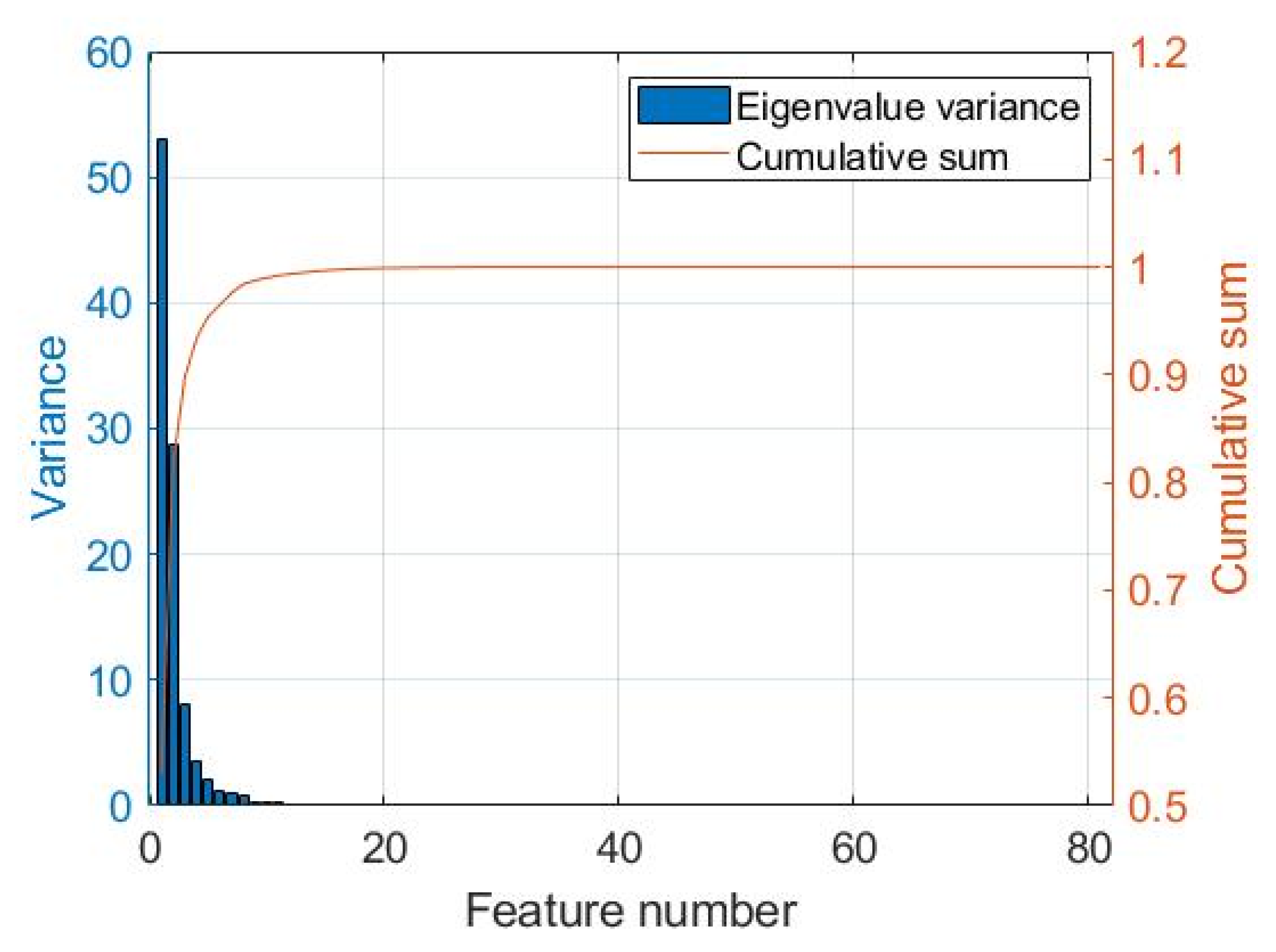
The PCA was applied to reduce the input-space dimensionality, thus allowing a more efficient ANN training. In Figure 18, the variance associated with each principal component of the detection dataset is presented, in which it is possible to see, by considering only the first 10 principal components, that it was possible to consider 99% of the total variance included in the dataset. As an example, six FFTs observed in presence of different damage extents were compared with their PCA reconstructions in Figure 19, specifically including just 10 out of 81 principal components. It is clear that a negligible error was made when considering the reduced input space when including the first 10 principal components only.

The classification ANN architecture included 10 input nodes, one binary output node, and 20 hidden nodes, with the latter defined based on trial-and-error procedure; however, as a compromise was made between training accuracy and generalization performance on test data never seen during training, to avoid overfitting. The ANN performances were synthetized with confusion matrices as shown in Figure 20, in which the similar performances in the training, validation, and test sets suggest the ANN possessed a high generalization capability, and no overfitting error occurred. Overall, less than 10% of misclassified examples were obtained.

Since the detection performance was tested in the presence of damages of increasing extent, thus with different influences on the simulated signal, it was interesting to verify the detection performance (in terms of the number of misclassified samples) as a function of the damage dimension. It is clear from

Table 5. Detailed detection ANN performance.

Equivalent Pitted Area	# Errors	Type
0	16/280	False alarm
0.2	20/56	Missed detection
0.35	13/56	Missed detection
0.48	4/56	Missed detection
0.63	0/56	Missed detection
1	0/56	Missed detection

that the probability for missed detection reasonably increased for smaller damages, while the detection performance improved with increasing damage entity.

3.3.2. Damage Localization

The dataset in

Table 6. Training-set composition for damage localization.

# Observations	Damage Radial Position	Units of Measure
92	12	mm
92	24	mm
92	36	mm

was used for localization ANN training; it was composed of 276 observation samples, including 81 features each. Also in this context, the PCA could be used to reduce the dataset dimensionality. It can be noticed in Figure 21 that more than 95% of the information within the signals was captured by considering the first 20 principal components of the dataset only.

Thus, the first 20 principal components of the dataset were used to train the regression ANN for damage localization. The network architecture included 20 input nodes, one output node describing the radial position of the damage as a continuous variable, and 10 hidden nodes, again defined in a way to avoid overfitting. The ANN performances are presented in Figure 22, in which the training, validation, and test regression plots are shown. As the increasing trend was correctly captured by the ANN in all the subsets, it was possible to conclude that the algorithm could generalize on new data, and no overfitting occurred. It is worth noticing that the entire dataset was processed by the algorithm in Figure 22a–c, including small damages with reduced sensitivity.

3.3.3. Damage Quantification

The same database used for localization was considered for damage quantification, specifically organized as in

Table 7. Training-set composition for damage quantification.

# Observations	Equivalent Pitted Area
55	0.2
55	0.35
55	0.48
55	0.63
55	1

, in view of data regression as a function of the damage extent. For this reason, the same conclusions could be drawn on the application of PCA, resulting in a reduction of the input space from ${ℝ}^{81}$ to ${ℝ}^{20}$. The regression ANN architecture included 21 input nodes, one output node describing the equivalent pitted area as a continuous variable, and 10 hidden nodes, again defined in a way to avoid overfitting. Focusing on the input layer, it included the first 20 PCA of the FFT calculated from the signal database, and one additional node collecting the damage location estimated by the previous diagnostic layer.

The ANN performances are presented in Figure 23. Specifically, Figure 23a–c show the training, validation, and test regression plots, while the correct damage location was passed as input to the network, verifying the correct data synthesis during algorithm training. However, while using the algorithm in a realistic scenario, one might argue that an erratic location can be provided as input to the algorithm, based on the performance of the localization ANN. For this reason, the quantification ANN was also tested while receiving as input the position estimation in Figure 22c, affected by errors, and results are shown in Figure 23d for the test subset only. When comparing Figure 23d with the corresponding Figure 23c, a reduction in algorithm precision was noticed, although the ANN could capture the trend with marked accuracy, demonstrating its potential for application in a realistic scenario.

4. Conclusions

A model-based approach to condition monitoring of gearbox transmissions was presented in this study, leveraging on a hybrid analytical–numerical model for the generation of signal examples to be used for algorithm training. The approach was applied to a back-to-back test rig, and experimental data in normal conditions were used to validate the baseline model and to extract realistic noise components to be superposed on numerically simulated signals. After a feature-extraction module used principal component analysis to project data in a more compact space dimension, these were passed as input to a hierarchical structure of artificial neural networks. A classification ANN was used for detection of pitting damage positioned on the teeth flank, intuitively manifesting better performances when signals in the presence of larger damages were processed. After damage was detected, two regression ANNs were used to correlate the variations of the signal FFT with the radial position of the damage and its severity. Specifically, it was found that an improved performance of the damage assessment algorithm was obtained while the information about damage position, estimated by the localization ANN, was passed to the network through an additional input node.

The algorithm performances were assessed at each level of the damage-identification hierarchy, and demonstrated to be extremely satisfactory, given the limited amount of simulations used to construct the training database, even in the presence of a realistic noise corrupting the ideal simulated data. Augmented accuracy and precision of the algorithm output was expected by increasing the density of the damage entity and position grids. However, considering the aim of this paper was to show the consistency of the approach, the adopted number of simulations was considered sufficient at this stage. Although the methodology described herein remains valid for any test configuration, it must be specified that the results obtained throughout this project were consistent and valid only for this bench test, since the digital model was coherent only with it, while a new database must be created for each examined scenario.

A final note must be made regarding the future developments of the project. It could be expanded by adding different damages to the simulation database; for example, including fatigue damage at the root of different teeth, or analyzing the effect of multiple simultaneous damages. However, while the combinations are endless, a perfectly tuned condition-monitoring system could be built only by investing a great amount of computational effort.