
Characterization of a Shallow Coastal Aquifer in the Framework of a Subsurface Storage and Soil Aquifer Treatment Project Using Electrical Resistivity Tomography (Port de la Selva, Spain)

 ,
,  ,
,  , and
, and
Abstract
:1. Introduction
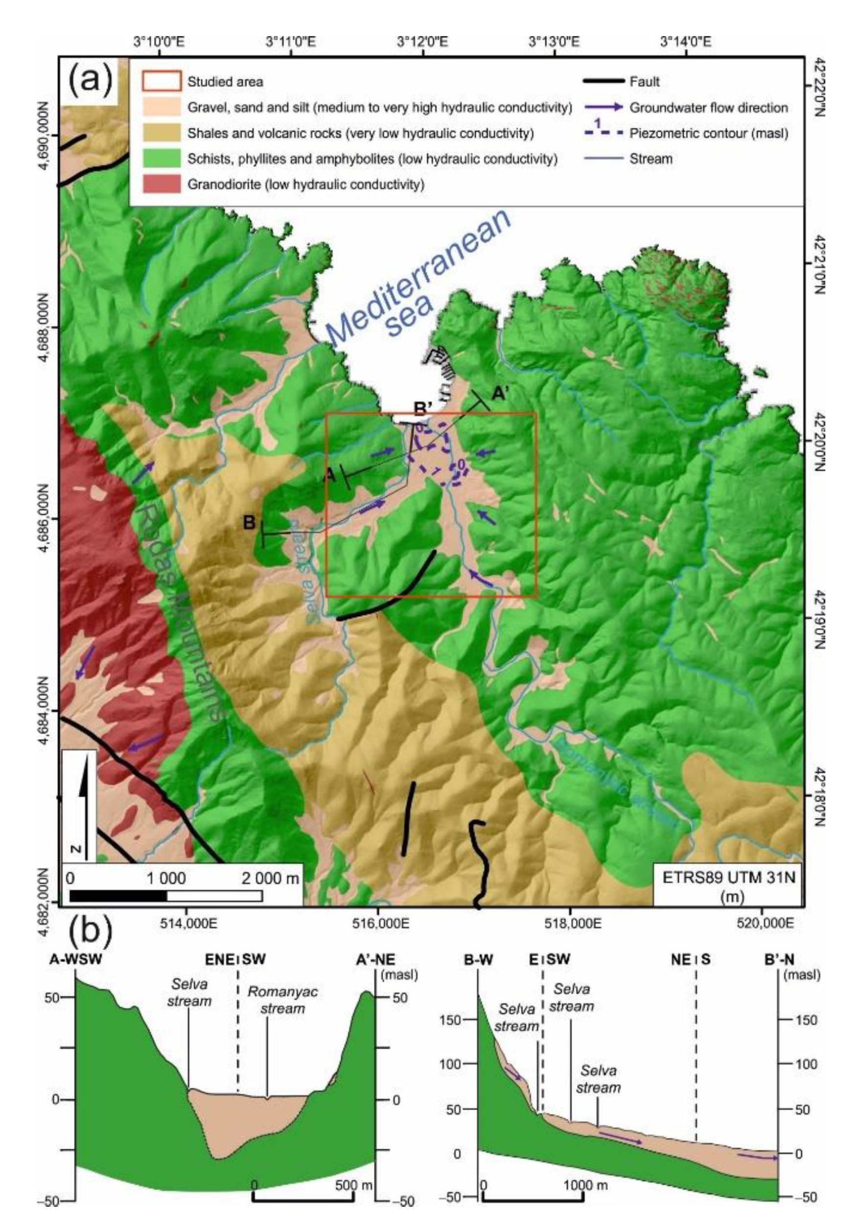
2. Study Area
2.1. Geographical, Climate, and Water Management Overview
2.2. Geological and Hydrogeological Setting
3. Materials and Methods
3.1. Electrical Resistivity Tomography
3.2. Electrical Resistivity Tomography Surveys
3.3. Aquifer Geometry and Saltwater Intrusion
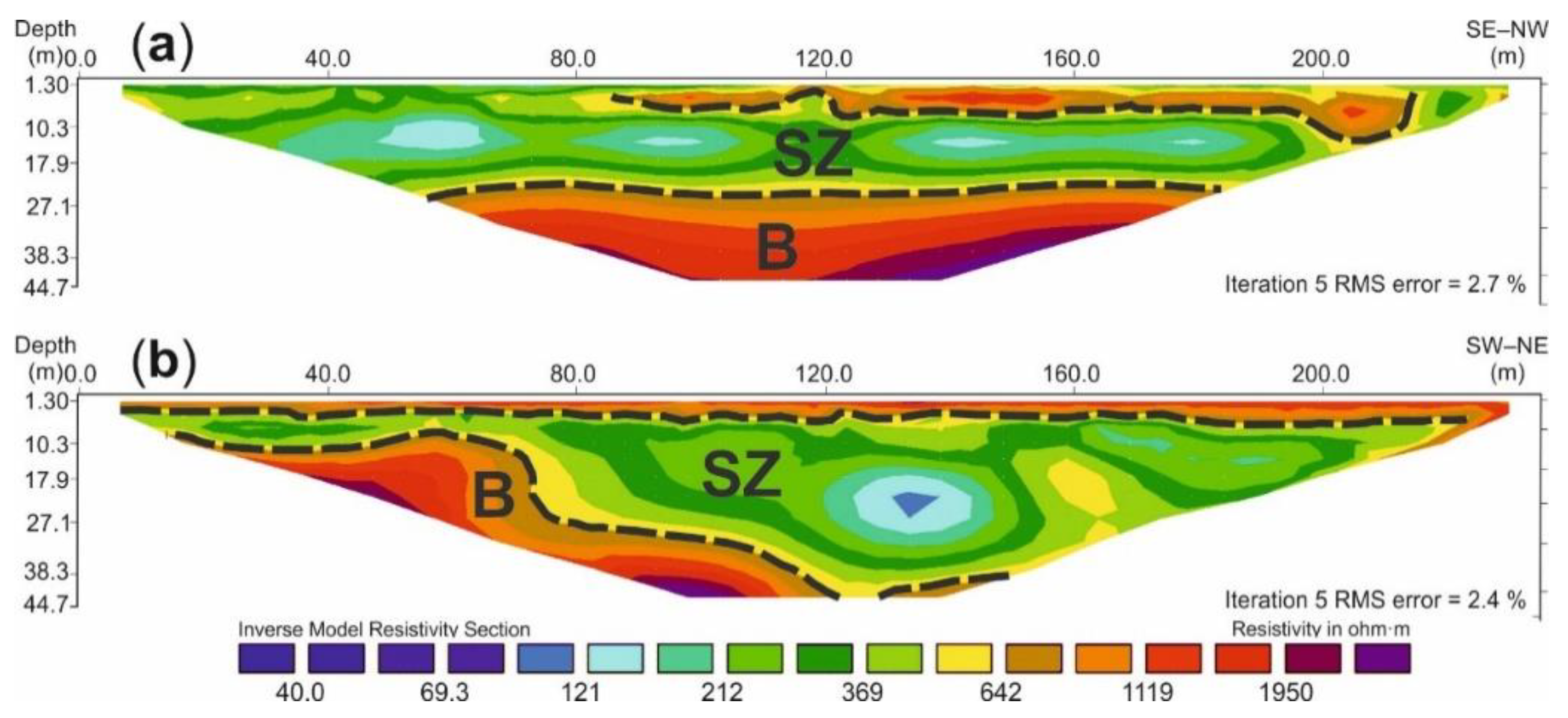
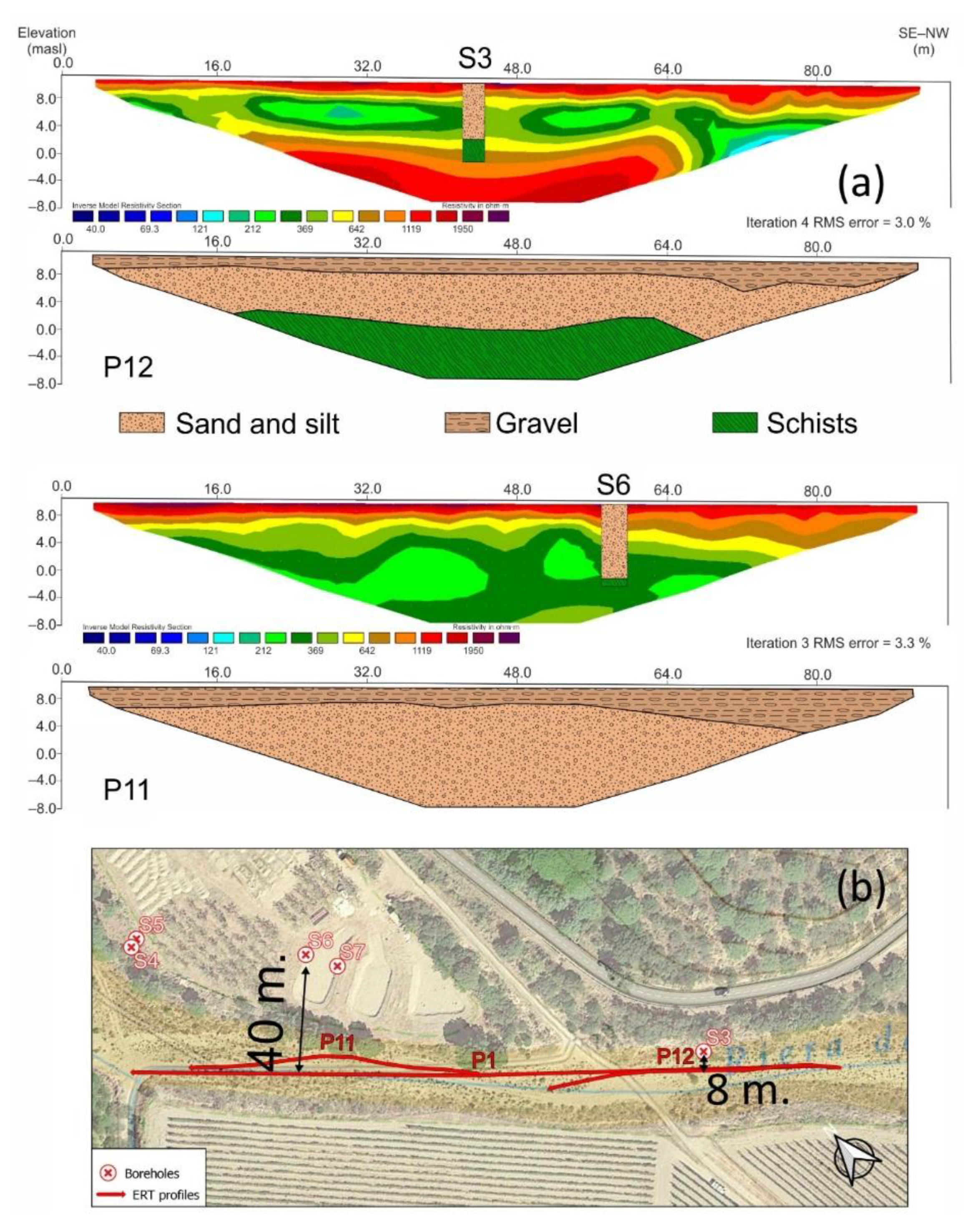
4. Results
4.1. Electrical Resistivity Models
4.2. Aquifer Geometry
4.3. Saltwater Intrusion
5. Discussion
5.1. Aquifer Geometry
5.2. Saltwater Intrusion
6. Conclusions
Author Contributions
Funding
Acknowledgments
Conflicts of Interest
References
- Van der Gun, J. Groundwater and Global Change: Trends, Opportunities and Challenges|International Groundwater Resources Assessment Centre; United Nations Educational, Scientific and Cultural Organization: Paris, France, 2012; ISBN 9789230010492. [Google Scholar]
- Aeschbach-Hertig, W.; Gleeson, T. Regional strategies for the accelerating global problem of groundwater depletion. Nat. Geosci. 2012, 5, 853–861. [Google Scholar] [CrossRef]
- Akbarpour, S.; Niksokhan, M.H. Investigating effects of climate change, urbanization, and sea level changes on groundwater resources in a coastal aquifer: An integrated assessment. Environ. Monit. Assess. 2018, 190. [Google Scholar] [CrossRef]
- Mastrocicco, M.; Colombani, N. The Issue of Groundwater Salinization in Coastal Areas of the Mediterranean Region: A Review. Water 2021, 13, 90. [Google Scholar] [CrossRef]
- Custodio, E. Coastal aquifers of Europe: An overview. Hydrogeol. J. 2010, 18, 269–280. [Google Scholar] [CrossRef]
- Alfarrah, N.; Walraevens, K. Groundwater overexploitation and seawater intrusion in coastal areas of arid and semi-arid regions. Water 2018, 10, 143. [Google Scholar] [CrossRef] [Green Version]
- Sabater, S.; Barceló, D. Water Scarcity in the Mediterranean: Perspectives under Global Change; Springer: Berlin, Germany, 2010; ISBN 978-3-642-03970-6(H). [Google Scholar]
- Marecos, M.H. Water reuse in Europe; Official Publication of the European Water Association (EWA): Hennef, Germany, 2007. [Google Scholar]
- Dillon, P.; Escalante, E.F.; Megdal, S.B.; Massmann, G. Managed aquifer recharge for water resilience. Water 2020, 12, 1846. [Google Scholar] [CrossRef]
- Angelakis, A.N.; Marecos Do Monte, M.H.F.; Bontoux, L.; Asano, T. The status of wastewater reuse practice in the Mediterranean basin: Need for guidelines. Water Res. 1999, 33, 2201–2217. [Google Scholar] [CrossRef]
- Dillon, P.; Pavelic, P.; Toze, S.; Rinck-Pfeiffer, S.; Martin, R.; Knapton, A.; Pidsley, D. Role of aquifer storage in water reuse. Desalination 2006, 188, 123–134. [Google Scholar] [CrossRef]
- Elkayam, R.; Sopliniak, A.; Gasser, G.; Pankratov, I.; Lev, O. Oxidizer Demand in the Unsaturated Zone of a Surface-Spreading Soil Aquifer Treatment System. Vadose Zone J. 2015, 14, 1–10. [Google Scholar] [CrossRef]
- Bekele, E.; Page, D.; Vanderzalm, J.; Kaksonen, A.; Gonzalez, D. Water recycling via aquifers for sustainable urban water quality management: Current status, challenges and opportunities. Water 2018, 10, 457. [Google Scholar] [CrossRef] [Green Version]
- Burris, D. Groundwater Replenishment System, 2019 Annual Report; Orange County Water District: Fountain Valley, CA, USA, 2020. [Google Scholar]
- De Carlo, L.; Caputo, M.C.; Masciale, R.; Vurro, M.; Portoghese, I. Monitoring the drainage efficiency of infiltration trenches in fractured and karstified limestone via time-lapse hydrogeophysical approach. Water 2020, 12, 2009. [Google Scholar] [CrossRef]
- Bekele, E.; Toze, S.; Patterson, B.; Higginson, S. Managed aquifer recharge of treated wastewater: Water quality changes resulting from infiltration through the vadose zone. Water Res. 2011, 45, 5764–5772. [Google Scholar] [CrossRef] [PubMed]
- Council, N.R. Ground Water Recharge Using Waters of Impaired Quality; The National Academies Press: Washington, DC, USA, 1994; ISBN 978-0-309-05142-2. [Google Scholar]
- Gale, I. Strategies for Managed Aquifer Recharge (MAR) in Semi-Arid Areas; International Association of Hydrogeologists commission on Management of Aquifer Recharge IAH-MAR, UNESCO Division of Water Sciences: Paris, France, 2005. [Google Scholar]
- Ringleb, J.; Sallwey, J.; Stefan, C. Assessment of managed aquifer recharge through modeling—A review. Water 2016, 8, 579. [Google Scholar] [CrossRef] [Green Version]
- EWRI. Standard Guidelines for Artificial Recharge of Ground Water; Environmental and Water Resources Institute, Ed.; Standards; American Society of Civil Engineers (ASCE): Reston, VA, USA, 2001; ISBN 978-0-7844-0548-2. [Google Scholar]
- Paz, M.C.; Alcalá, F.J.; Medeiros, A.; Martínez-Pagán, P.; Pérez-Cuevas, J.; Ribeiro, L. Integrated MASW and ERT imaging for geological definition of an unconfined alluvial aquifer sustaining a coastal groundwater-dependent ecosystem in southwest Portugal. Appl. Sci. 2020, 10, 5905. [Google Scholar] [CrossRef]
- González-Quirós, A.; Comte, J.C. Relative importance of conceptual and computational errors when delineating saltwater intrusion from resistivity inverse models in heterogeneous coastal aquifers. Adv. Water Resour. 2020, 144, 103695. [Google Scholar] [CrossRef]
- Behroozmand, A.A.; Auken, E.; Knight, R. Assessment of Managed Aquifer Recharge Sites Using a New Geophysical Imaging Method. Vadose Zone J. 2019, 18, 1–13. [Google Scholar] [CrossRef] [Green Version]
- Binley, A.; Hubbard, S.S.; Huisman, J.A.; Revil, A.; Robinson, D.A.; Singha, K.; Slater, L.D. The emergence of hydrogeophysics for improved understanding of subsurface processes over multiple scales. Water Resour. Res. 2015, 51, 3837–3866. [Google Scholar] [CrossRef] [Green Version]
- Drahor, M.G.; Berge, M.A.; Göktürkler, G.; Kurtulmuş, T.Ö. Mapping aquifer geometry using electrical resistivity tomography: A case study from Şanlıurfa, south-eastern Turkey. Near Surf. Geophys. 2011, 9, 55–66. [Google Scholar] [CrossRef]
- Benabdelouahab, S.; Salhi, A.; Himi, M.; Stitou El Messari, J.E.; Casas Ponsati, A. Geoelectrical investigations for aquifer characterization and geoenvironmental assessment in northern Morocco. Environ. Earth Sci. 2019, 78, 1–16. [Google Scholar] [CrossRef]
- Sendrós, A.; Himi, M.; Lovera, R.; Rivero, L.; Garcia-Artigas, R.; Urruela, A.; Casas, A. Geophysical Characterization of Hydraulic Properties around a Managed Aquifer Recharge System over the Llobregat River Alluvial Aquifer (Barcelona Metropolitan Area). Water 2020, 12, 3455. [Google Scholar] [CrossRef]
- Martínez, J.; Benavente, J.; García-Aróstegui, J.L.; Hidalgo, M.C.; Rey, J. Contribution of electrical resistivity tomography to the study of detrital aquifers affected by seawater intrusion-extrusion effects: The river Vélez delta (Vélez-Málaga, southern Spain). Eng. Geol. 2009, 108, 161–168. [Google Scholar] [CrossRef]
- Galazoulas, E.C.; Mertzanides, Y.C.; Petalas, C.P.; Kargiotis, E.K. Large Scale Electrical Resistivity Tomography Survey Correlated to Hydrogeological Data for Mapping Groundwater Salinization: A Case Study from a Multilayered Coastal Aquifer in Rhodope, Northeastern Greece. Environ. Process. 2015, 2, 19–35. [Google Scholar] [CrossRef] [Green Version]
- Kazakis, N.; Pavlou, A.; Vargemezis, G.; Voudouris, K.S.; Soulios, G.; Pliakas, F.; Tsokas, G. Seawater intrusion mapping using electrical resistivity tomography and hydrochemical data. An application in the coastal area of eastern Thermaikos Gulf, Greece. Sci. Total Environ. 2016, 543, 373–387. [Google Scholar] [CrossRef]
- Hasan, M.; Shang, Y.; Jin, W.; Shao, P.; Yi, X.; Akhter, G. Geophysical Assessment of Seawater Intrusion into Coastal Aquifers of Bela Plain, Pakistan. Water 2020, 12, 3408. [Google Scholar] [CrossRef]
- Vann, S.; Puttiwongrak, A.; Suteerasak, T.; Koedsin, W. Delineation of seawater intrusion using geo-electrical survey in a coastal aquifer of Kamala beach, Phuket, Thailand. Water 2020, 12, 506. [Google Scholar] [CrossRef] [Green Version]
- Lajaunie, C.; Courrioux, G.; Manuel, L. Foliation fields and 3D cartography in geology: Principles of a method based on potential interpolation. Math. Geol. 1997, 29, 571–584. [Google Scholar] [CrossRef]
- SMC. Climatologia. L’Alt Empordà. 1961–2000; Servei Meteorològic de Catalunya—Departament de Medi Ambient i Habitatge, Generalitat de Catalunya: Barcelona, Spain, 2014. [Google Scholar]
- Bayer-Raich, M.; Vilanova, E.; Jordana, S. Water reuse in El Port de la Selva: Groundwater modelling of Soil Aquifer Treatment (SAT) for reclaimed water. In Proceedings of the 5th International Symposium RE-WATER Braunschweig, Braunschweig, Germany, 2–3 November 2015; pp. 158–174. [Google Scholar]
- Fajnorová, S.; Sprenger, C.; Hermes, N.; Ternes, T.A.; Sala, L.; Miehe, U.; Drewes, J.E.; Hübner, U. Assessment of Full-Scale Indirect Potable Water Reuse in El Port de la Selva, Spain. Water 2021, 13, 325. [Google Scholar] [CrossRef]
- MPR Real Decreto 140/2003, de 7 de Febrero, por el que se Establecen los Criterios Sanitarios de la Calidad del Agua de Consumo Humano. Ministerio de la Presidencia Gobierno de España. Available online: http://www.boe.es/boe/dias/2003/02/21/pdfs/A07228-07245.pdf (accessed on 21 January 2021).
- Martinez, X.; Hochstrat, R.; Miehe, U.; Casado, F.; Frijns, J.; Bortoli, J.; Denieul, M.P.; Orsoni, J.; Alcalde, L.; Jeffrey, J.; et al. Final Report: DEMOWARE (Innovation Demonstration for a Competitive and Innovative European Water Reuse Sector); Community Research and Development Information Service (CORDIS): Luxembourg, 2017. [Google Scholar]
- Sprenger, C.; Kraus, F.; Schwarzmüller, H.; Miehe, U.; Bayer, M.; Vilanova, E. Pretreatment requirements and design guidelines for SAT technologies, and two SAT case studies. El Port de la Selva. In DEMOWARE (Innovation Demonstration for a Competitive and Innovative European Water Reuse Sector); Community Research and Development Information Service (CORDIS): Luxembourg, 2017; pp. 100–163. [Google Scholar]
- Druguet, E. The Structure of the NE Cap de Creus Peninsula Relationships with Metamorphism and Magmatism. Ph.D Thesis, Universitat Autònoma de Barcelona, Barcelona, Spain, 1997. [Google Scholar]
- ICGC. Alt Empordà. Mapa Geològic Comarcal de Catalunya 1:50 000; Institut Cartogràfic i Geològic de Catalunya: Barcelona, Spain, 2006. [Google Scholar]
- ICGC. Mapa Hidrogeològic de Roses, Cap de Creus i Far de Creus 1:25 000; Institut Cartogràfic i Geològic de Catalunya: Barcelona, Spain, 2013. [Google Scholar]
- ICGC. Mapa Hidrogeològic de Llança 1:25 000; Institut Cartogràfic i Geològic de Catalunya: Barcelona, Spain, 2013. [Google Scholar]
- Dahlin, T. 2D resistivity surveying for environmental and engineering applications. First Break 1996, 14, 275–284. [Google Scholar] [CrossRef] [Green Version]
- Sasaki, Y. Resolution of Resistivity Tomography inferred from numerical simulation. Geophys. Prospect. 1992, 40, 453–463. [Google Scholar] [CrossRef]
- Loke, M.H.; Barker, R.D. Rapid least-squares inversion of apparent resistivity pseudosections by a quasi-Newton method. Geophys. Prospect. 1996, 131–152. [Google Scholar] [CrossRef]
- Loke, M.H.; Dahlin, T. A comparison of the Gauss–Newton and quasi-Newton methods in resistivity imaging inversion. J. Appl. Geophys. 2002, 49, 149–162. [Google Scholar] [CrossRef] [Green Version]
- Ellis, R.G.; Oldenburg, D.W. Applied geophysical inversion. Geophys. J. Int. 1994, 116, 5–11. [Google Scholar] [CrossRef] [Green Version]
- Oyeyemi, K.D.; Aizebeokhai, A.P.; Adagunodo, T.A.; Olofinnade, O.M.; Sanuade, O.A.; Olaojo, A.A. Subsoil characterization using geoelectrical and geotechnical investigations: Implications for foundation studies. Int. J. Civ. Eng. Technol. 2017, 8, 302–314. [Google Scholar]
- Everett, M.E. Electrical resistivity method. In Near-Surface Applied Geophysics; Cambridge University Press: Cambridge, UK, 2013; pp. 70–103. ISBN 9781139088435. [Google Scholar]
- Martorana, R.; Fiandaca, G.; Casas Ponsati, A.; Cosentino, P.L. Comparative tests on different multi-electrode arrays using models in near-surface geophysics. J. Geophys. Eng. 2009, 6, 101–110. [Google Scholar] [CrossRef] [Green Version]
- Dahlin, T.; Zhou, B. A numerical comparison of 2D resistivity imaging with 10 electrode arrays. Geophys. Prospect. 2004, 52, 379–398. [Google Scholar] [CrossRef] [Green Version]
- Rey, J.; Martínez, J.; Mendoza, R.; Sandoval, S.; Tarasov, V.; Kaminsky, A.; Hidalgo, M.C.; Morales, K. Geophysical characterization of aquifers in southeast spain using ERT, TDEM, and vertical seismic reflection. Appl. Sci. 2020, 10, 7365. [Google Scholar] [CrossRef]
- Seequent. User Manual for Leapfrog Geo version 6.0; Seequent Limited: Christchurch, New Zealand, 2020. [Google Scholar]
- Hardy, R.L. Multiquadric equations of topography and other irregular surfaces. J. Geophys. Res. 1971, 76, 1905–1915. [Google Scholar] [CrossRef]
- Carlson, R.E.; Foley, T.A. Interpolation of track data with radial basis methods. Comput. Math. Appl. 1992, 24, 27–34. [Google Scholar] [CrossRef] [Green Version]
- Franke, R. Scattered Data Interpolation: Tests of Some Method. Math. Comput. 1982, 38, 181–200. [Google Scholar] [CrossRef]
- Piret, C.; Dissanayake, N.; Gierke, J.S.; Fornberg, B. The Radial Basis Functions Method for Improved Numerical Approximations of Geological Processes in Heterogeneous Systems. Math. Geosci. 2020, 52, 477–497. [Google Scholar] [CrossRef]
- Cowan, E.J.; Beatson, R.K.; Fright, W.R.; Mclennan, T.J.; Mitchell, T.J. Rapid geological modelling. In Proceedings of the Applied Structural Geology for Mineral Exploration and Mining, International Symposium, Kalgoorlie, Australia, 23–25 September 2002; pp. 1–9. [Google Scholar]
- Alhuri, Y.; Ouazar, D.; Taik, A. Radial Basis Functions Alternative Solutions to Shallow Water Equations. Front. Sci. Eng. 2011, 1, 25–40. [Google Scholar]
- Scheuerer, M.; Schaback, R.; Schlather, M. Interpolation of spatial data-A stochastic or a deterministic problem? Eur. J. Appl. Math. 2013, 24, 601–629. [Google Scholar] [CrossRef] [Green Version]
- Hillier, M.J.; Schetselaar, E.M.; de Kemp, E.A.; Perron, G. Three-Dimensional Modelling of Geological Surfaces Using Generalized Interpolation with Radial Basis Functions. Math. Geosci. 2014, 46, 931–953. [Google Scholar] [CrossRef]
- Houlding, S.W. 3D Geoscience Modeling; Springer: Berlin/Heidelberg, Germany, 1994; ISBN 978-3-642-79014-0. [Google Scholar]
- Vollgger, S.A.; Cruden, A.R.; Ailleres, L.; Cowan, E.J. Regional dome evolution and its control on ore-grade distribution: Insights from 3D implicit modelling of the Navachab gold deposit, Namibia. Ore Geol. Rev. 2015, 69, 268–284. [Google Scholar] [CrossRef]
- Cowan, E.J. Deposit-scale structural architecture of the Sigma-Lamaque gold deposit, Canada—insights from a newly proposed 3D method for assessing structural controls from drill hole data. Miner. Depos. 2020, 55, 217–240. [Google Scholar] [CrossRef] [Green Version]
- Beatson, R.K.; Cherrie, J.B.; Mouat, C.T. Fast fitting of radial basis functions: Methods based on preconditioned GMRES iteration. Adv. Comput. Math. 1999, 11, 253–270. [Google Scholar] [CrossRef]
- Cowan, E.J.; Beatson, H.J.; Ross, H.J.; Fright, W.R.; McLennan, T.J.; Evans, T.R.; Carr, J.C.; Lane, R.G.; Bright, D.V.; Gillman, A.J.; et al. Practical Implicit Geological Modelling. In Proceedings of the 5th International Mining Geology Conference, Victoria, Australia, 17–19 November 2003; The Australasian Institute of Mining and Metallurgy: Carlton Victoria, Australia, 2003; pp. 89–99. [Google Scholar]
- Guo, J.; Wang, J.; Wu, L.; Liu, C.; Li, C.; Li, F.; Lin, M.; Jessell, M.W.; Li, P.; Dai, X.; et al. Explicit-implicit-integrated 3-D geological modelling approach: A case study of the Xianyan Demolition Volcano (Fujian, China). Tectonophysics 2020, 795, 228648. [Google Scholar] [CrossRef]
- Sherif, M.; El Mahmoudi, A.; Garamoon, H.; Kacimov, A.; Akram, S.; Ebraheem, A.; Shetty, A. Geoelectrical and hydrogeochemical studies for delineating seawater intrusion in the outlet of Wadi Ham, UAE. Environ. Geol. 2006, 49, 536–551. [Google Scholar] [CrossRef]
- Abdul Nassir, S.S.; Loke, M.H.; Lee, C.Y.; Nawawi, M.N.M. Salt-water intrusion mapping by geoelectrical imaging surveys. Geophys. Prospect. 2000, 48, 647–661. [Google Scholar] [CrossRef]
- Song, S.H.; Lee, J.Y.; Park, N. Use of vertical electrical soundings to delineate seawater intrusion in a coastal area of Byunsan, Korea. Environ. Geol. 2007, 52, 1207–1219. [Google Scholar] [CrossRef]
- Chafouq, D.; El Mandour, A.; Elgettafi, M.; Himi, M.; Bengamra, S.; Lagfid, Y.; Casas, A. Assessing of Saltwater Intrusion in Ghiz-Nekor Aquifer (North Morocco) Using Electrical Resistivity Tomography. In Proceedings of the Near Surface Geoscience 2016—22nd European Meeting of Environmental and Engineering Geophysics, Barcelona, Spain, 4–8 September 2016; Volume 2016. Available online: https://0-doi-org.brum.beds.ac.uk/10.3997/2214-4609.201602066 (accessed on 30 December 2020).
- Kura, N.U.; Ramli, M.F.; Ibrahim, S.; Sulaiman, W.N.A.; Zaudi, M.A.; Aris, A.Z. A preliminary appraisal of the effect of pumping on seawater intrusion and upconing in a small tropical island using 2D resistivity technique. Sci. World J. 2014, 2014. [Google Scholar] [CrossRef] [PubMed] [Green Version]
- Rubin, Y.; Hubbard, S.S. Hydrogeophysics; Springer: Dordrecht, The Netherlands, 2005; ISBN 978-1-4020-3101-4. [Google Scholar]
- de Marsily, G.; Delay, F.; Gonçalvès, J.; Renard, P.; Teles, V.; Violette, S. Dealing with spatial heterogeneity. Hydrogeol. J. 2005, 13, 161–183. [Google Scholar] [CrossRef]
- Chen, J.; Hubbard, S.S.; Gaines, D.; Korneev, V.; Baker, G.; Watson, D. Stochastic estimation of aquifer geometry using seismic refraction data with borehole depth constraints. Water Resour. Res. 2010, 46, W11539. [Google Scholar] [CrossRef]
- Ghiglieri, G.; Buttau, C.; Arras, C.; Funedda, A.; Soler, A.; Barbieri, M.; Carrey, R.; Domènech, C.; Torrentó, C.; Otero, N.; et al. Using a multi-disciplinary approach to characterize groundwater systems in arid and semi-arid environments: The case of Biskra and Batna regions (NE Algeria). Sci. Total Environ. 2020, 757, 143797. [Google Scholar] [CrossRef] [PubMed]
- APHA. Standard Methods for the Examination of Water and Wastewater, 20th ed.; Clesceri, L., Greenberg, A., Eaton, A., Eds.; American Public Health Association: Washington, DC, USA, 1999; ISBN 0-87553-235-7. [Google Scholar]


| ID | Number of Profiles | Length (m) | Electrode Interval (m) | Orientation to Water Stream |
|---|---|---|---|---|
| P1 and P2 | 2 | 235 | 5 | parallel and transverse |
| P3 | 1 | 188 | 4 | oblique |
| P4, P5 and P6 | 3 | 235 | 5 | parallel and transverse |
| P7 | 1 | 94 | 2 | transverse |
| P8 | 1 | 235 | 5 | parallel |
| P9 and P10 | 2 | 235 | 5 | transverse and parallel |
| P11 and P12 | 2 | 94 | 2 | parallel |
| P13 to P17 | 5 | 235 | 5 | transverse, parallel and oblique |
| Physicochemical Parameter | Units | 2017 | 2018 | 2019 | WHO Range for Aquifers 1 | RD 14/2013 2 | ||
|---|---|---|---|---|---|---|---|---|
| Fresh | Brackish | Saline | ||||||
| Na+ | (mg/L) | 361 | >1000 | >1000 | <200 | 200–400 | >400 | 200 |
| K+ | (mg/L) | 9 | 67 | 30 | <55 | 55–70 | >70 | — |
| Cl− | (mg/L) | 683 | 8518 | 4329 | <250 | 250–1000 | >1000 | 250 |
| SO42− | (mg/L) | 129 | 1008 | 536 | <200 | 200–500 | >500 | 250 |
| EC 3 | (µS/cm) | 2315 | 24,271 | 12,342 | <1500 | 1500–3000 | >3000 | 2500 |
Publisher’s Note: MDPI stays neutral with regard to jurisdictional claims in published maps and institutional affiliations. |
© 2021 by the authors. Licensee MDPI, Basel, Switzerland. This article is an open access article distributed under the terms and conditions of the Creative Commons Attribution (CC BY) license (http://creativecommons.org/licenses/by/4.0/).
Share and Cite
Sendrós, A.; Urruela, A.; Himi, M.; Alonso, C.; Lovera, R.; Tapias, J.C.; Rivero, L.; Garcia-Artigas, R.; Casas, A. Characterization of a Shallow Coastal Aquifer in the Framework of a Subsurface Storage and Soil Aquifer Treatment Project Using Electrical Resistivity Tomography (Port de la Selva, Spain). Appl. Sci. 2021, 11, 2448. https://0-doi-org.brum.beds.ac.uk/10.3390/app11062448
Sendrós A, Urruela A, Himi M, Alonso C, Lovera R, Tapias JC, Rivero L, Garcia-Artigas R, Casas A. Characterization of a Shallow Coastal Aquifer in the Framework of a Subsurface Storage and Soil Aquifer Treatment Project Using Electrical Resistivity Tomography (Port de la Selva, Spain). Applied Sciences. 2021; 11(6):2448. https://0-doi-org.brum.beds.ac.uk/10.3390/app11062448
Chicago/Turabian StyleSendrós, Alex, Aritz Urruela, Mahjoub Himi, Carlos Alonso, Raúl Lovera, Josefina C. Tapias, Luis Rivero, Ruben Garcia-Artigas, and Albert Casas. 2021. "Characterization of a Shallow Coastal Aquifer in the Framework of a Subsurface Storage and Soil Aquifer Treatment Project Using Electrical Resistivity Tomography (Port de la Selva, Spain)" Applied Sciences 11, no. 6: 2448. https://0-doi-org.brum.beds.ac.uk/10.3390/app11062448