
Optimizing Support Locations in the Roof–Column Structural System


1
School of Architecture and Urban Planning, Nanjing University, Nanjing 210093, China
2
Centre for Innovative Structures and Materials, School of Engineering, RMIT University, Melbourne 3001, Australia
3
Centre of Translational Atomaterials, Faculty of Science, Engineering and Technology, Swinburne University of Technology, Hawthorn 3122, Australia
*
Author to whom correspondence should be addressed.
Appl. Sci. 2021, 11(6), 2775; https://0-doi-org.brum.beds.ac.uk/10.3390/app11062775
Submission received: 26 February 2021
/
Revised: 15 March 2021
/
Accepted: 15 March 2021
/
Published: 19 March 2021
(This article belongs to the Special Issue Toward Sustainable Engineering Structures for Better Safety in Built-Environment)
Abstract
:The roof–column structural system is utilized for many engineering and architectural applications due to its structural efficiency. However, it typically requires column locations to be predetermined, and involves a tedious trial-and-error adjusting process to fulfil both engineering and architectural requirements. Finding efficient column distributions with the aid of computational methods, such as structural optimization, is an ongoing challenge. Existing methods are limited, with continuum methods involving the generation of undesired complex shapes, and discrete methods involving a time-consuming process for optimizing columns’ spatial order. This paper presents a new optimization method to design the distribution of a given number of vertical supporting columns under a roof structure. A computational algorithm was developed on the basis of the optimality-criterion (OC) method to preserve and removed candidate columns pre-embedded with design requirements. Three substrategies are presented to improve optimizer performance. The effectiveness of the new method was validated with a range of roof–column structural models. Treating column locations as design variables provides opportunities to significantly improve structural performance.
1. Introduction
The roof–column structural system creates a simple form of shelter. It is utilized across many architectural and engineering applications due to its effectiveness in supporting environmental loads, transmitting the structure’s weight, and reducing solar heat gains [1]. However, determining locations of supporting columns under the roof is a challenging task; they have direct influence on both architectural appearance and structural performance.
The integrated structural–architectural design was suggested to be an effective strategy for capturing complex requirements from both engineering and architectural perspectives [2]. This includes the utilization of structural optimization, where the optimization design process achieves specific objectives by changing defined design variables. For example, a curved frame’s minimal size and shape can be designed with a given applied load through optimization [3]. Many other applications were all enabled by extensive preceding work in structural optimization using diverse structural optimization methods [4], including continuum and discrete techniques.
Continuum methods obtain optimal designs by determining the shapes and locations of cavities in continuous geometries [5,6]. Many popular topology optimization methods are part of continuum methods, including the homogenization approach [7], the solid isotropic material with penalization (SIMP) method [8,9,10], the bidirectional evolutionary structural optimization (BESO) method [11,12,13,14], and the level set method [15,16,17]. Although those continuum methods can maximize the stiffness of a structure with specified design constraints, it is difficult to apply them in roof–column structural systems to find optimal locations of predefined columns, as they include the generation of complex 3D shapes. For example, the iconic Qatar National Convention Center, designed using the extended ESO method, has complex treelike columns supporting a simple rectangular roof [18].
Discrete methods obtain optimal designs by determining the optimal spatial order and connectivity of line-based representations, such as trusses, frames, and equilibrium configurations of tensegrity structures [19,20,21,22]. They typically involve the utilization of computational algorithms, such as the genetic algorithm (GA) [23], the simulated annealing (SA) algorithm [24], and particle swarm optimization (PSO) [25]. The key benefit of using discrete methods is that components in optimal designs can be predetermined, thereby being widely utilized in structural designs such as space frames with standard member types [26]. However, existing discrete methods can be computationally expensive due to many candidate elements, and require a user-defined objective function for optimization problems that can be difficult to formulate and implement.
This paper proposes a new integrated structural–architectural design method for automatically finding optimal column locations in roof–column structural systems. The new method combines the objective function from topology optimization for compliance minimization with a discrete design domain comprising candidate-supporting columns, thus capturing architectural requirements and ensuring structural performance. Section 2 describes an optimization algorithm for implementing the new method. Section 3 introduces three substrategies for controlling the optimization tendency in order to obtain improved results. Section 4 validates the proposed method using a square-roof example. Section 5 presents research implications using two additional examples with nonregular roof shapes, followed by a conclusion in Section 6.
2. Optimal Column Locations
2.1. Problem Definition
This paper combines structural analysis with predetermined vertical columns to find efficient layout distribution of a prescribed number of columns under a flat roof. Predetermined columns are defined as a predefined column type and allowable locations where the column type is determined from a given length, Young’s modulus, and cross-sectional shape.
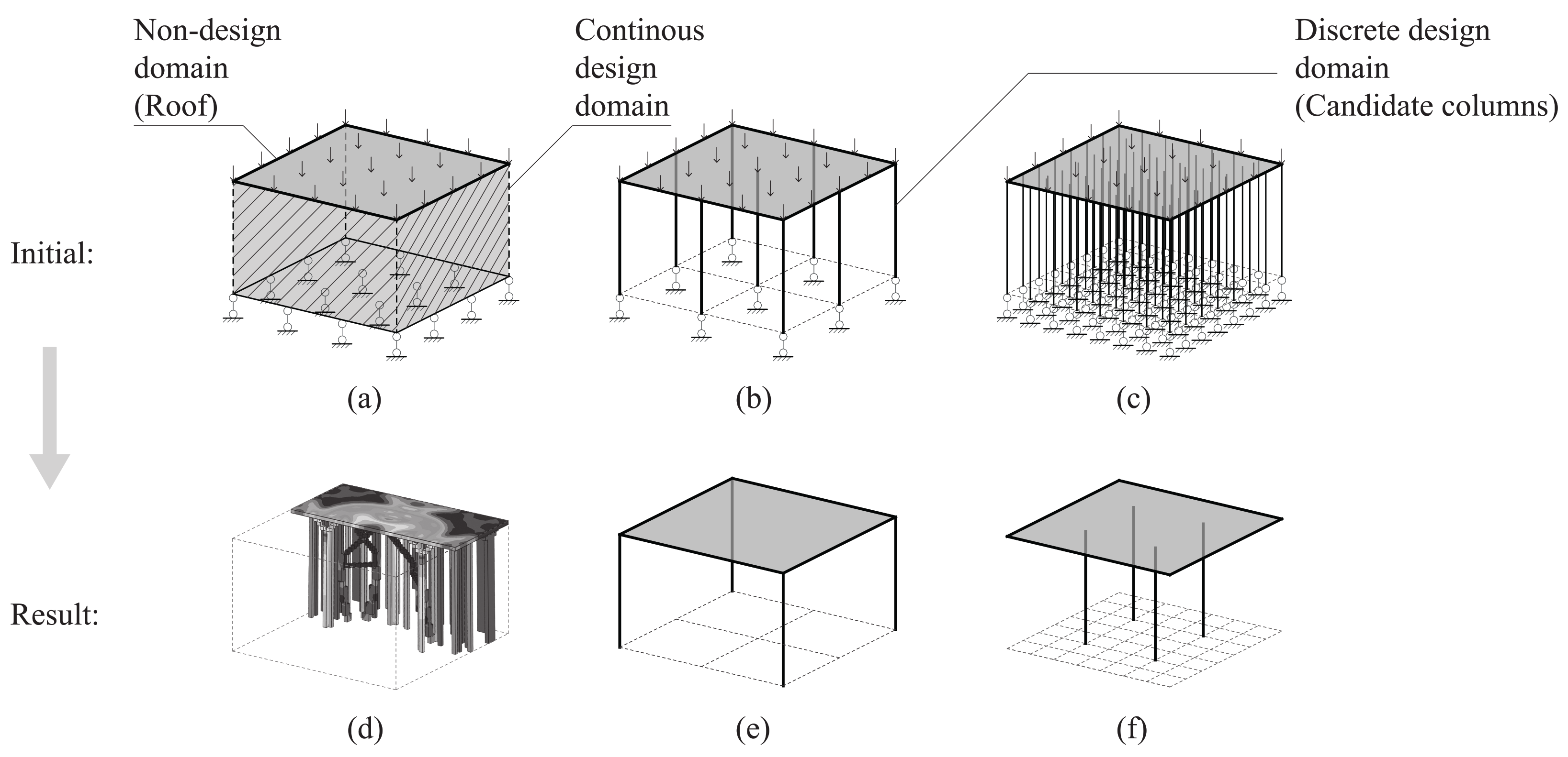
This section first reviews the limitation of previous methods and introduces the critical advantages of the new method. Figure 1 shows a comparison between a typical continuum method and the proposed method using the same roof, loading, and boundary conditions. The BESO method was selected for representing continuum methods. The BESO result includes columns with different sizes and shapes, obtained by adding and removing efficient and inefficient elements, respectively, as shown in Figure 1a,d. The critical limitation of the BESO method lies in the fact that the optimizer cannot control the shape of generated columns. Hence, the BESO method is not suitable for the present problem to realize specified design requirements.
In contrast to continuum methods, the new method can embed design requirements in the initialization stage using a grid of predetermined columns under the roof, as shown in Figure 1b,c. In this setup, vertical lines and the planar surface represent columns and the roof, respectively. As shown in Figure 1e,f, optimization results preserve a prescribed number of columns and remove other predetermined columns. Different candidate columns can lead to different final distributions. The following subsections describe the details of the new optimization method.
2.2. Problem Statement
The optimization problem can be considered as stiffness maximization (or compliance minimization) of the overall roof–column system with constraints determining the number of columns. The mathematical problem statement can be written as follows.
where compliance C is the objective function that is the inverse measure of the overall stiffness of a structure; and are the global force vector and displacement vector, respectively; is the design variable denoting the relative density of the i-th column; is a small value declaring the absence of a column; and is the global stiffness matrix. Equation (4) is an additional constraint that ensures the equilibrium of the structure.
2.3. Optimization Algorithm
The optimality-criterion (OC) method is an effective strategy to vary all candidate data on the basis of a given hypothesis [27]. Solving the optimization problem using the OC method can simultaneously preserve and remove efficient and inefficient columns. In this paper, columns were hinged, so they were only loaded in the axial direction; the columns’ axial tress represents the OC method’s candidate data. The relative density of columns can vary continuously between and 1, as described in Equation (3), and the summation of all design variables must be equal to a prescribed number, as described in Equation (2). The optimization process is repeated until the structural system’s compliance is minimized, which gives clear column distribution where the optimization result includes preserved and removed columns, with being approximately 1 and 0, respectively. Details of the optimization algorithm are as follows.
The initial design variable of columns, , is first defined as the ratio of the prescribed number of columns elements, , to the number of candidate columns N, representing that specified column materials are uniformly distributed to all candidate columns:
Various methods can solve the optimization problem [28,29]. The OC method [9,27] was selected in this paper for updating design variable , which can be written as
where denotes the i-th design variable at the k-th iteration, is the move limit, is a numerical damping coefficient, and determines the optimality condition, which can be defined as
where is a Lagrange multiplier, and is the axial stress of the i-th column at the k-th iteration. Equation (7) is valid because: (i) is set to consider all elastic strain energy behaviors, , generated from the i-th column, but the column only generated axial stress. (ii) The magnitude of does not affect the optimization result due to the utilization of the Lagrange multiplier, . That is to say, Equation (7) is obtained by simplifying Equations (8) and (9) with the consideration of (i) and (ii).
where is Young’s modulus of the predetermined columns.
Lagrange multiplier in Equations (6) and (7) can be determined using a bisection method to enforce the constraint stated in Equation (2) during optimization;
where and are the lower and upper bound limits, respectively. In the bisection method, it was assumed that < < . To this end, is almost always zero, and is a large constant. The bounds are updated according to the summation of current design variables: if , the lower bound is updated to be ; if , the upper bound is updated to be . The bisectional iterative process is repeated until , meaning , which satisfies the constraint stated in Equation (3).
When design variable is updated from Equations (6)–(10), the Young’s modulus of columns in a roof–column structural system is determined using the penalization method. This represents that columns’ axial stiffness can continuously vary throughout optimization depending on relative density.
where is the Young’s modulus of the i-th column at the k-th iteration and p is the penalty exponent. The utilization of Equation (11) enforces the final design variable of columns to be approximately 1 or 0 with p selected to be 3. When = 1, preserved columns have a design Young’s modulus ( = ). When 0, removed columns have a near-zero Young’s modulus ( 0), corresponding to a near-zero axial stiffness.
The above algorithm provides a basic framework enabling all columns’ design variable to be effectively and simultaneously updated for finding an optimal distribution of a prescribed number of columns using the optimality-criterion method on the basis of their axial stress. Three substrategies are introduced in the following section to improve the optimization result by systemically controlling the optimization tendency.
3. Controlling Optimization Tendency
3.1. Initial Discrete Candidates
The first substrategy considers the loading area of candidate columns determined by their initial locations, where columns with a small and large loading area tend to be removed and preserved, respectively. This can be demonstrated more clearly using 8 × 8 and 6 × 6 candidate columns under the same roof with = 4, as shown in Figure 2a,b, respectively. Their final column distributions were different because of the variation of their initial loading areas around the roof edges. Corner candidate columns in Figure 2b correspond to a larger loading area, hence generating higher elastic-strain energy since early iterations during optimization tend to be preserved according to Equation (6). The compliance of Figure 2b was approximately twice larger than that of Figure 2a, suggesting that a local optimal solution was found. This paper considered all candidate columns under the roof, including columns on roof edges, to avoid local optimal solutions caused by edge columns in the following examples.
3.2. Roof–Column Relative Stiffness
The second substrategy characterizes the optimization problem, and considers constant relative stiffness between roof and columns. This method was previously demonstrated by [30], with constant relative stiffness being enforced during optimization to ensure that the algorithm was solving the equivalent structural system in every iteration. In this study, implementing constant relative stiffness can effectively improve the optimization result, as the columns’ axial stiffness can vary throughout optimization to give different structural systems. This can be achieved by using a material interpolation scheme in the roof region with the consideration of the penalty exponent, meaning that the roof’s stiffness can vary throughout optimization.
where and are the Young’s modulus of the roof at the k-th iteration and the initial state, respectively. Therefore, relative stiffness between roof and columns is determined as , which can be used for characterizing optimization problem and structural system. in the optimization result, as is satisfied with the utilization of Equation (2), representing that the roof’s Young’s modulus is the same in the first and final iteration.
3.3. Filtering Scheme
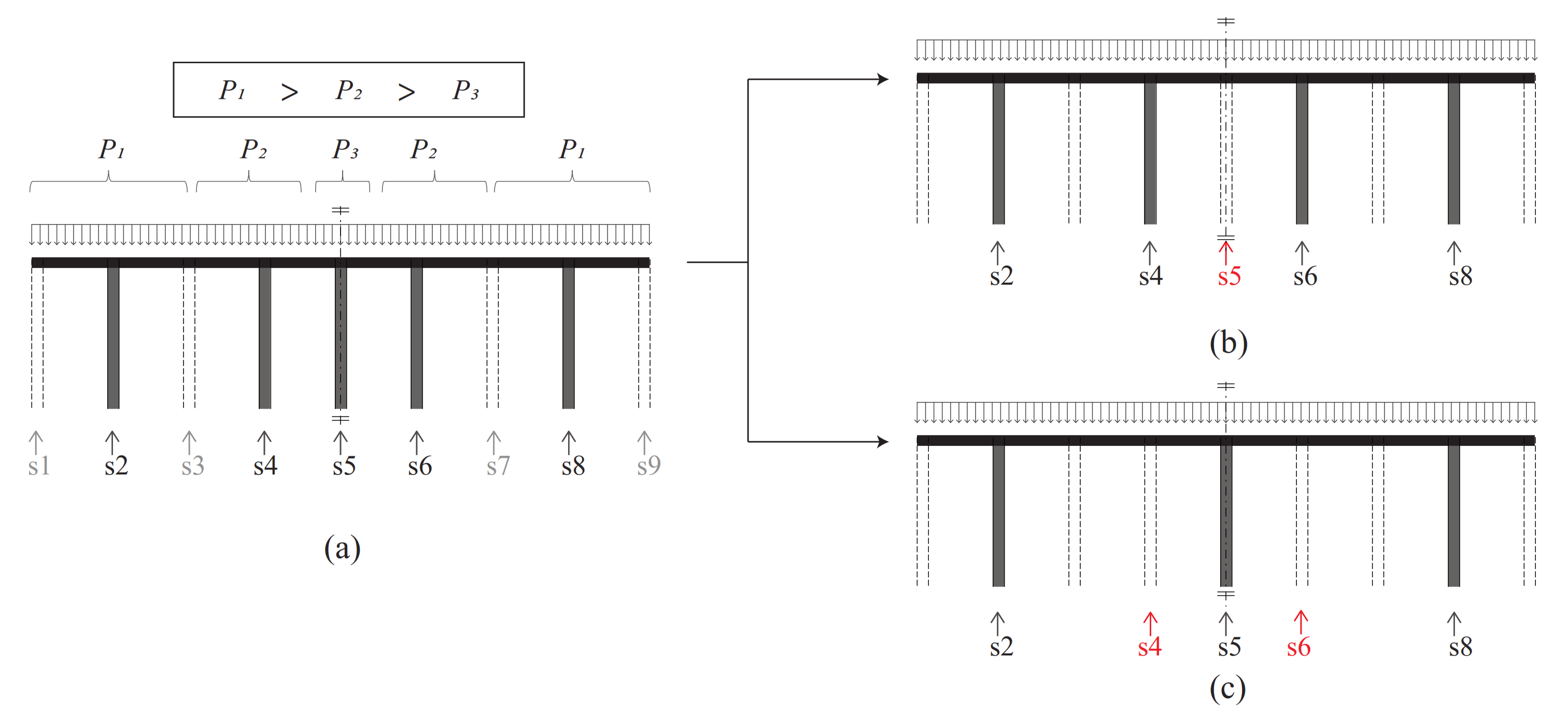
The third and final substrategy considers a filter in the optimization algorithm that can be used for producing a grid-independent solution and influencing optimization tendency [4]. This is illustrated using a 2D roof–column example in Figure 3. Figure 3a represents an intermediate state of an optimization process, with 5 columns being preserved from 9 candidate columns. The 5 remaining columns correspond to a different portion of a uniformly distributed load (), where are supported by Columns s2 and s8, are supported by Columns s4 and s6, and is supported by column s5. As mentioned in Section 3.1, columns with a smaller loading area tend to be removed first. Therefore, the optimization algorithm obtains the solution by removing Column s5, as shown in Figure 3b. A filtering technique was introduced for blurring and smoothing the loading information of columns, which enabled the columns located on the symmetric axis (s5) with a small loading area to be preserved without losing solution accuracy, as shown in Figure 3c.
The filter was formulated using the distance between columns as the weight factor to smooth the axial stress of columns.
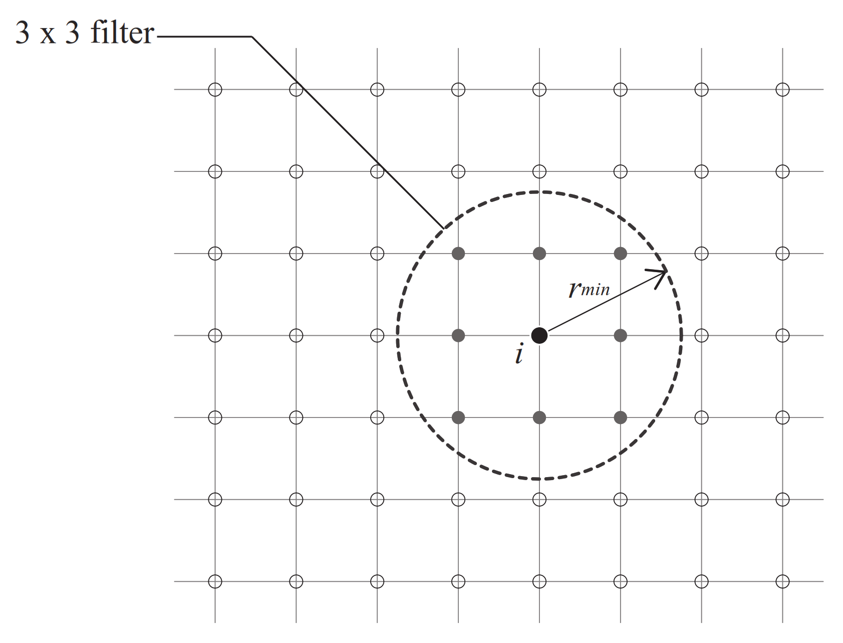
where is the linear weight factor, is the distance between column centers i and j, and is the filter radius, as shown in Figure 4. This paper only considered a 3 × 3 filter for the i-th column in the grid, which is the smallest filtering size, able to capture information of its 8 surrounding columns. The filter was only employed when a clear distribution of columns was obtained, as it is used for optimizing the locations of well-defined columns, as demonstrated in Figure 3. However, the definition of well-defined columns is mathematically vague in intermediate optimization states. The filtering condition was then set by introducing a parameter . This required the axial stress of columns to be ranked on the basis of their magnitude from high to low. The filter was employed if the summation of axial stress from the first of N columns exceeded 50% of total axial stress (), where . This paper utilizes the filtering technique in the following examples. The effect of different is explored in the next section.
4. Numerical Analysis
4.1. Method
To validate the proposed optimization method, numerical finite-element models were created in commercial software Abaqus, and the computational optimization algorithm was implemented using Python code. An implicit static general analysis method was used for structural analysis during optimization. Roof surfaces were meshed with quadrangular S4 shell elements, and columns were simulated using line or beam elements located on mesh nodes. Intersections of roof–columns and columns–ground were set to be pin connections. This was achieved by using tie constraints to connect the roof (shell) with all candidate columns (lines); both ends of the columns were only subject to translation constraints. Roofs were subject to uniformly distributed loads. Materials were modelled to be linearly elastic without consideration of plasticity. Young’s moduli for roofs and columns were 63.5 and 210 GPa, respectively. Poisson’s ratio for both materials was set to be 0.3. The mass density of roofs and columns was 2500 and 7800 kg/m3, respectively. The optimization solver considered all three improved techniques introduced in Section 3.
4.2. Optimization Results
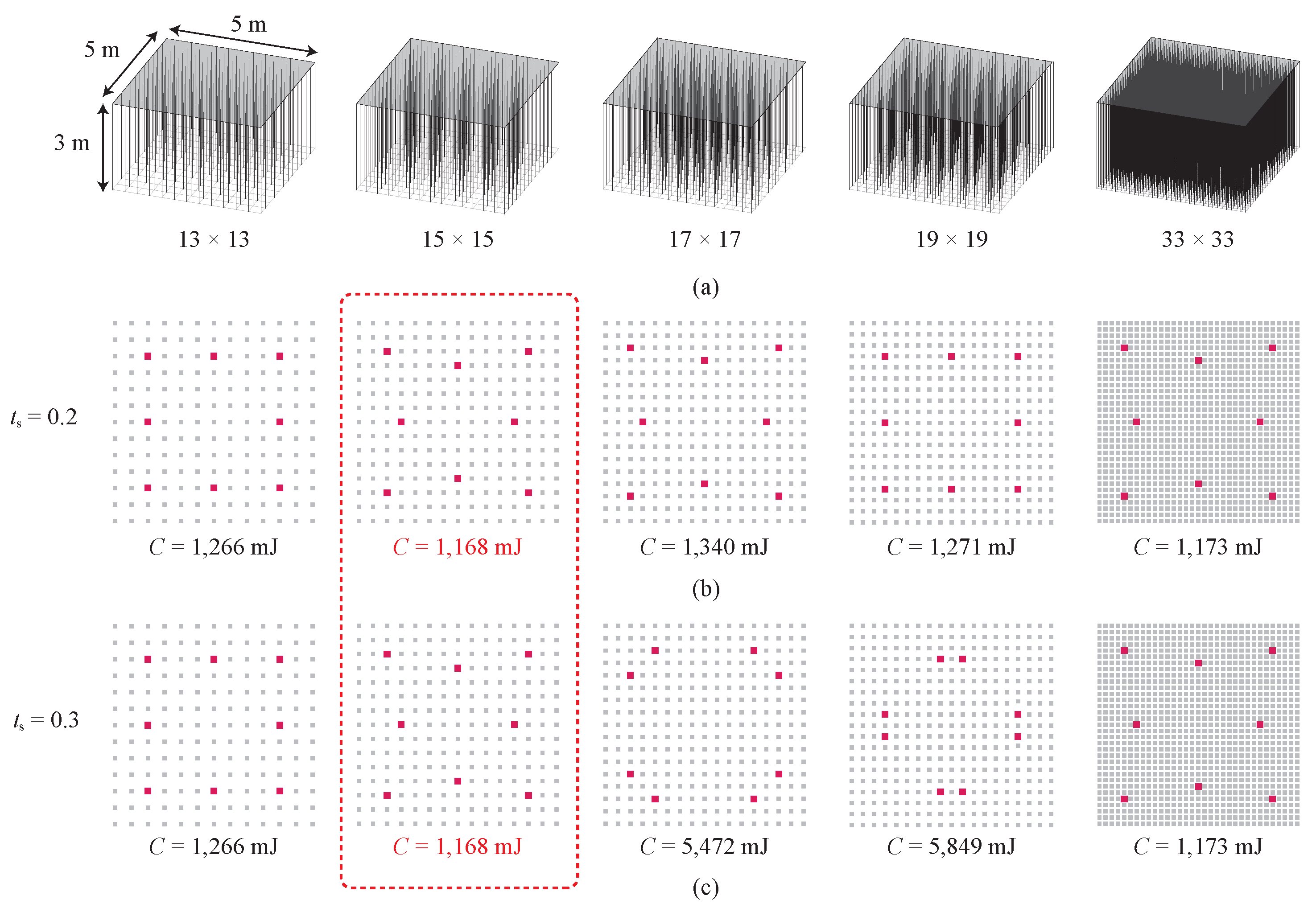
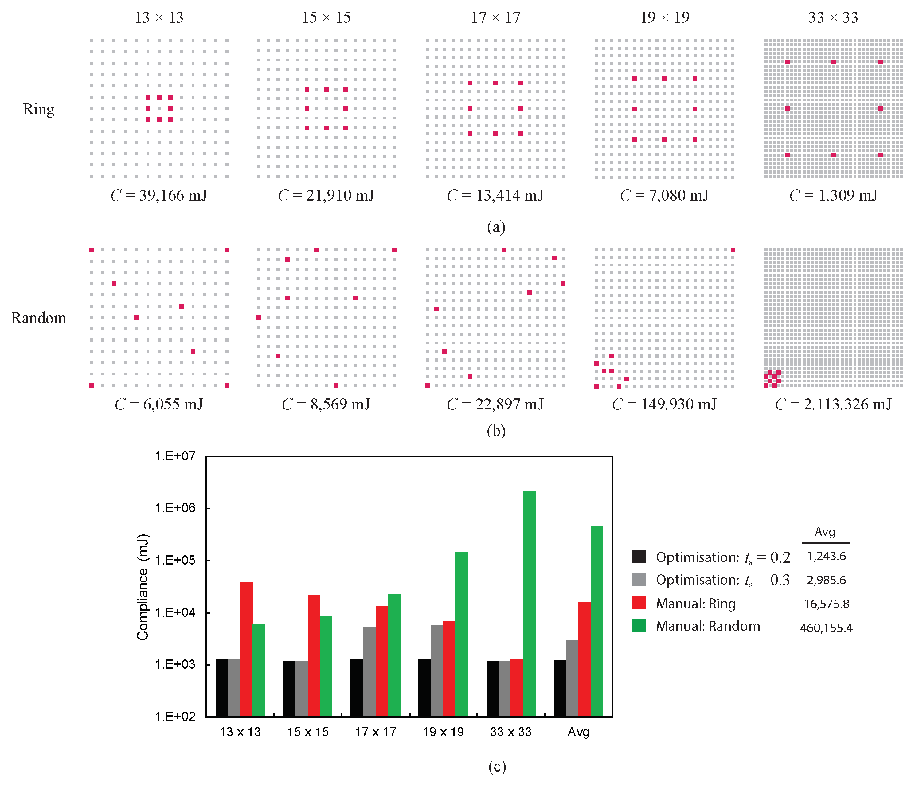
The entire optimization process was first tested using a simple 5 × 5 × 3 m design domain, which included a 100 mm thick square roof, and discrete candidate columns with a predetermined solid square cross-section of 100 × 100 mm, as shown in Figure 5a. The optimization solver searched for locations of = 8 columns under the square roof. Different candidate columns were tested, including a grid of 13 × 13, 15 × 15, 17 × 17, 19 × 19, and 33 × 33 columns. The filtering condition was tested for = 0.2 and 0.3, as shown in Figure 5b,c, respectively.
On the basis of the observed results in Figure 5b,c, variation in the number and locations of candidate columns could lead to different final distributions of the 8 prescribed columns. The selection of changes the optimization solution. When an appropriate is selected, such as 0.2, similar final distributions of columns can be obtained from different candidate configurations, as shown in Figure 5b. On the other hand, when is selected to be 0.3, diverse final distributions of columns can be generated to enrich architectural diversity, as shown in Figure 5c. Although those diverse results may not guarantee global minimal compliance from an engineering perspective, the new optimization method is still an effective tool for finding unexpected optimal distributions of columns under a roof from a large number of potential combinations, which is highly beneficial from an integrated structural–architectural design point of view. Optimization results are further examined in the following subsection.
4.3. Result Validation
To demonstrate the efficiency of the proposed method, optimization results from Figure 5 are compared with manual results in Figure 6, which were generated from user-defined column locations arranged in “ring” and random configurations, as shown in Figure 6a,b, respectively. The ring-configuration selection was due to the shape similarity to the optimization results possessing small compliance in Figure 5. Small-to-large rings were tested, and the purpose of utilizing manual ring configurations was to systemically examine whether the optimization solver had obtained a near-global optimal solution, as highlighted in Figure 5. Furthermore, the utilization of random configurations demonstrated that there were many other potential combinations of column locations, representing a tedious trial-and-error process.
Compliance comparison across different methods is summarized in Figure 6c. First, it was confirmed that the optimization solver successfully obtained a near-global optimal solution using 15 × 15 candidate columns, which had the smallest compliance across all tests. This suggests that a parametric study may be needed if the global optimal solution is part of the design requirements for future applications. Second, the compliance of random tests was much greater than that of the optimization results. The averaged compliance of random tests from Figure 6b was approximately 370 and 154 times larger than the optimization results from Figure 5b ( = 0.2) and Figure 5c ( = 0.3), respectively. This again confirmed the efficiency of the optimization method for automatically finding column locations and avoiding extremely large compliance.
The proposed method is therefore effective in enabling the rapid design of column locations under a flat roof, which has high potential to be combined with complex architectural designs, including irregular roof shapes, discussed in the following section.
5. Extended Designs
5.1. Eye-Shaped Roof
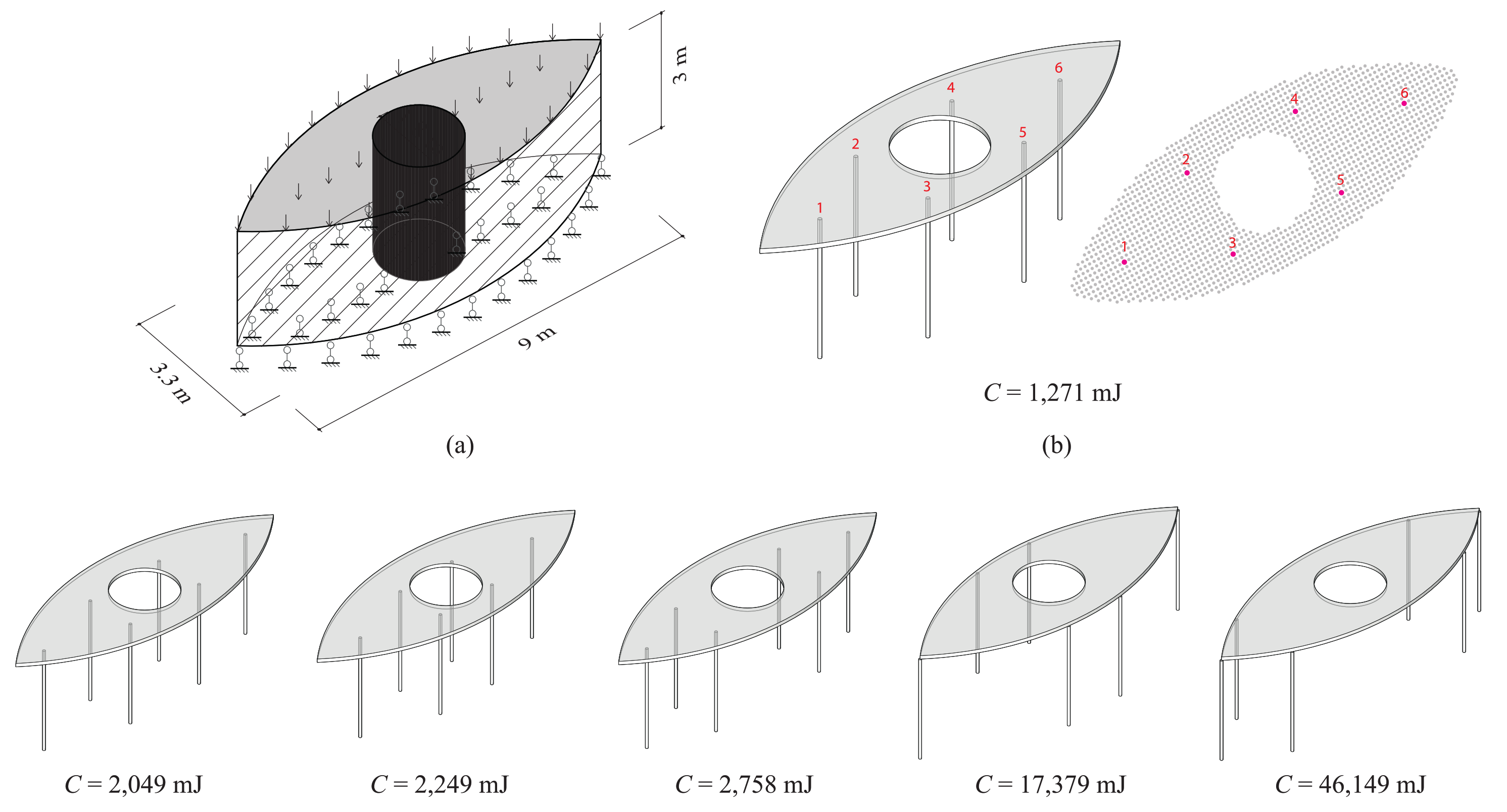
The shape of the eye-shaped roof, as shown in Figure 7a, was inspired by Santiago Calatrava’s works [31]. The new optimization algorithm was used for finding locations of = 6 columns in a 3.3 × 9 × 3 m design domain. The eye-shaped roof had a thickness of 100 mm. A total of 1712 candidate columns were used, which had a predetermined circular section with a 37.5 mm radius and 5 mm wall thickness. was 0.2, and other parameters were set to be the same as those in Section 4.
The optimization result is shown in Figure 7b, which had the lowest compliance compared with a set of manual results, as shown in Figure 7c. This demonstrates a high degree of design efficiency in finding column locations under a complex roof shape to obtain improved structural performance. A more complicated roof shape with a nonsymmetrical profile is examined in the following subsection.
5.2. Bean-Shaped Roof
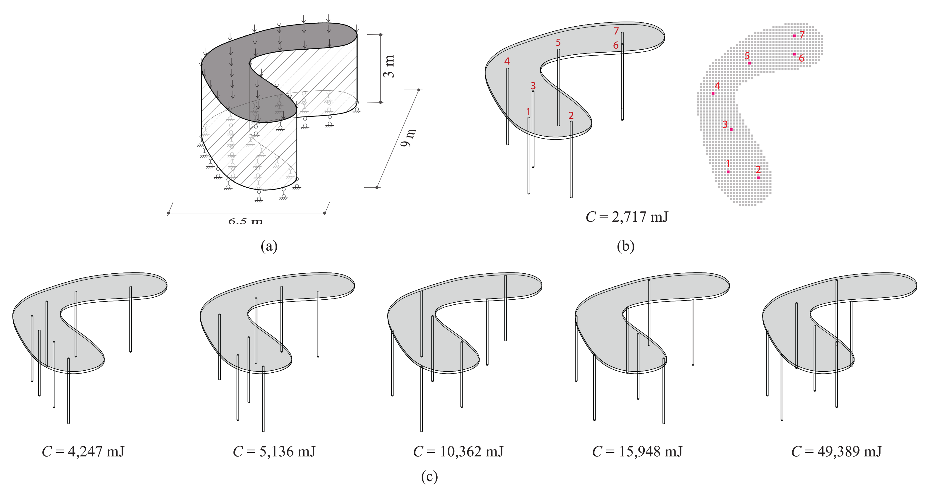
The bean-shaped roof, as shown in Figure 8a, was inspired by Kazuyo Sejima’s designs [32]. The optimization algorithm was used for finding locations of = 7 columns in a 9 × 6.5 × 3 m design domain. A total of 1159 candidate columns were used with a square cross-section of 100 × 100 mm. Other parameters were unchanged from those in the previous example.
5.3. Pavilion with Bean-Shaped Roof
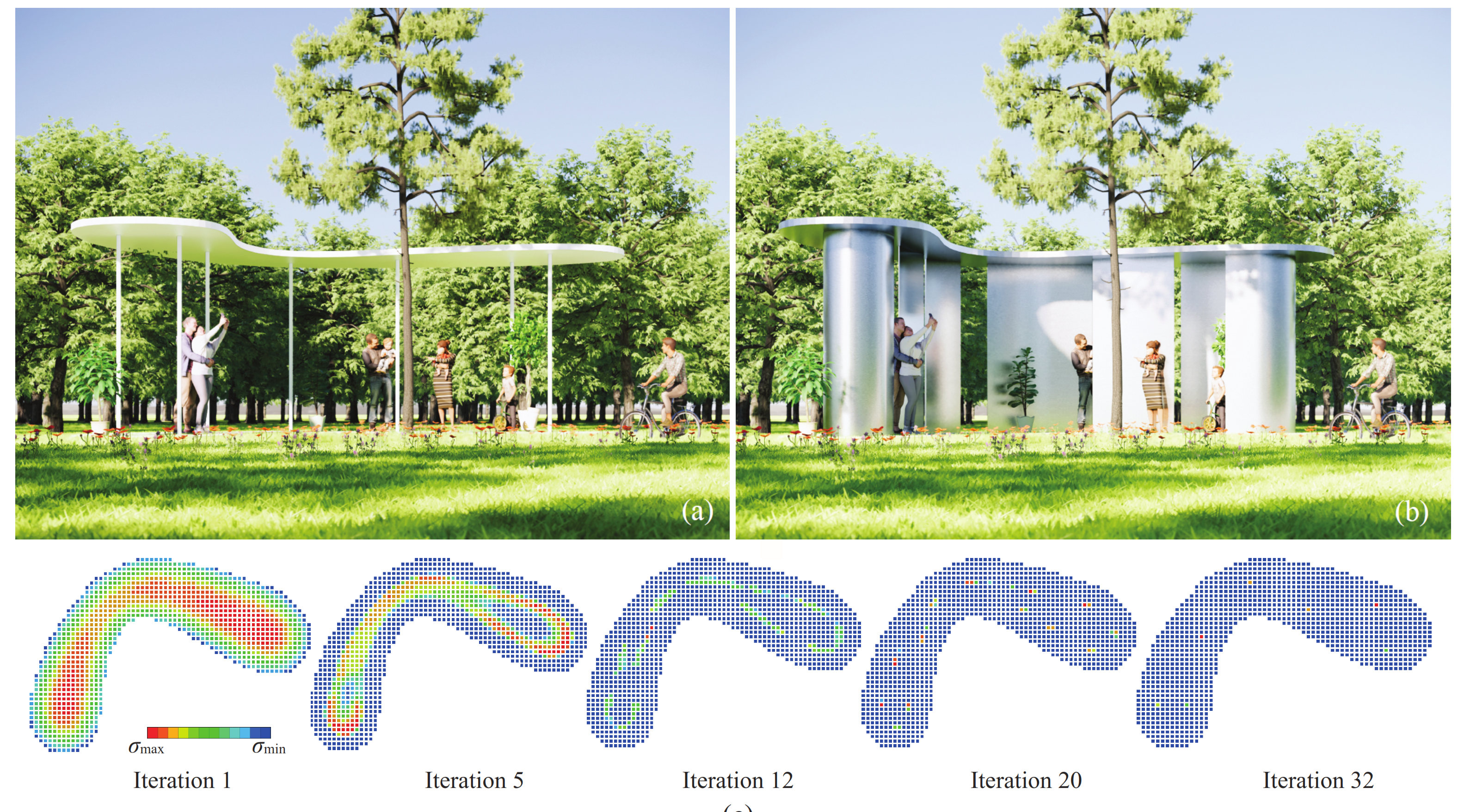
This paper proposes a new pavilion design based on a bean-shaped roof’s optimization result for demonstrating research implications, as shown in Figure 9. Figure 9a shows that a simple roof–column structural system is capable of providing adequate protection against environmental loads and sunlight. Column locations fulfil both engineering and architectural requirements, where structural performance was optimized and analyzed using the finite-element method, and the number of columns and their allowable locations were predetermined by the designer. Furthermore, curved panels can be installed under the roof to increase the level of protection, as shown in Figure 9b. The proposed optimization method offers a new method for determining shapes and locations of curved panels on the basis of a selected intermediate state’s stress distribution. For example, curved panels in Figure 9b was designed by connecting locations of high-stress columns at the 12th iteration, as shown in Figure 9c. However, further study is needed to develop this.
5.4. Discussion
The investigation into efficient column locations under flat roofs showed that the proposed method could effectively remove inefficient candidate columns. Allowable locations depend on the roof’s mesh layout, where columns were connected to the grid points; a finer mesh corresponds to a large number of candidate columns. Examples in Section 5.1 and Section 5.2 both had over 1000 candidate columns. However, computational costs were low. The OC method allowed for both examples to obtain their results within 1 hour using less than 100 iterations.
This study considered compliance minimization of a roof–column structural system without considering the roof’s deflection. However, stiffer results (with smaller compliance values) may correspond to smaller deflections, which may be achieved using more support columns. If deflection limitations are part of the design requirements, minimizing roof deflection can also be formulated as a different objective function. Simultaneously minimizing the compliance of the structural system and roof deflection may require a multiobjective optimization algorithm. Future study is needed to develop this.
6. Conclusions
This study presented a new optimization method to design column locations under a flat roof. The new method was developed on the basis of the optimality-criterion (OC) algorithm, which allowed for all columns’ relative density to be simultaneously updated throughout optimization. The optimality condition was set on the basis of the columns’ axial stress, as columns were hinged and only loaded in the axial direction. Three substrategies were developed to improve optimizer performance. First, adjusting locations of candidate columns gives different loading areas, where columns with small and large loading areas tend to be removed and preserved, respectively. Second, enforcing constant relative stiffness between roof and columns ensures that the algorithm solves the equivalent structural system during optimization. Third, employing a filter can result in a grid-independent solution without losing solution accuracy. The key finding of this study is that optimizing column locations significantly reduces structure compliance.
The new method was validated using a variety of roof–column structural models ranging from simple to complex roof shapes: square, eye-shaped, and bean-shaped roofs. The optimization algorithm was highly capable of finding efficient column layout distributions from a large number of potential combinations. Manual column location analysis was carried out to confirm that the optimizer had successfully obtained optimal designs. Lastly, this paper demonstrated the practical application of the proposed method in a pavilion design.
Author Contributions
Conceptualization, Y.M.X.; methodology, Y.M.X., X.H., and X.M.; software, X.M. and Y.X.; validation, Y.M.X. and X.H.; formal analysis, T.-U.L.; investigation, X.M.; data curation, X.M. and X.H.; writing—original-draft preparation, X.M. and T.-U.L.; writing—review and editing, T.-U.L. and Y.M.X.; visualization, X.M.; supervision, Y.M.X.; project administration, Y.M.X.; funding acquisition, X.M. and Y.M.X. All authors have read and agreed to the published version of the manuscript.
Funding
This project was funded by the Australian Research Council (FL190100014), the China Scholarship Council (201906195003), and the National Natural Science Foundation of China (51778283).
Institutional Review Board Statement
Not applicable.
Informed Consent Statement
Not applicable.
Data Availability Statement
The results of the optimized designs and the basic code of this work are available from the corresponding author on reasonable request.
Conflicts of Interest
The authors declare that they have no known competing financial interests or personal relationships that could have appeared to influence the work reported in this paper.
References
- Charleson, A. Structure as Architecture; Routledge: London, UK, 2014. [Google Scholar]
- Adriaenssens, S.; Block, P.; Veenendaal, D.; Williams, C. (Eds.) Shell Structures for Architecture: Form Finding and Optimization; Routledge: London, UK, 2014. [Google Scholar]
- Michell, A.G.M. The limits of economy of material in frame-structures. Philos. Mag. 1904, 8, 589–597. [Google Scholar] [CrossRef] [Green Version]
- Huang, X.; Xie, Y.M. Evolutionary Topology Optimization of Continuum Structures: Methods and Applications; Wiley: Chichester, UK, 2010. [Google Scholar]
- Stromberg, L.L.; Beghini, A.; Baker, W.F.; Paulino, G.H. Application of layout and topology optimization using pattern gradation for the conceptual design of buildings. Struct. Multidiscip. Optim. 2011, 43, 165–180. [Google Scholar] [CrossRef] [Green Version]
- Turnbull, J. Toyo Ito: Forces of Nature; Princeton Architectural Press: New York, NY, USA, 2012. [Google Scholar]
- Bendsøe, M.P.; Kikuchi, N. Generating optimal topologies in structural design using a homogenization method. Comput. Methods Appl. Mech. Eng. 1988, 71, 197–224. [Google Scholar] [CrossRef]
- Bendsøe, M.P. Optimal shape design as a material distribution problem. Struct. Optim. 1989, 1, 193–202. [Google Scholar] [CrossRef]
- Zhou, M.; Rozvany, G.I.N. The COC algorithm, part II: Topological, geometrical and generalized shape optimization. Comput. Methods Appl. Mech. Eng. 1991, 89, 309–336. [Google Scholar] [CrossRef]
- Bendsøe, M.P.; Sigmund, O. Material interpolation schemes in topology optimization. Arch. Appl. Mech. 1999, 69, 635–654. [Google Scholar] [CrossRef]
- Xie, Y.M.; Steven, G.P. A simple evolutionary procedure for structural optimization. Comput. Struct. 1993, 49, 885–896. [Google Scholar] [CrossRef]
- Querin, O.M.; Steven, G.P.; Xie, Y.M. Evolutionary structural optimisation (ESO) using a bidirectional algorithm. Eng. Comput. 1998, 15, 1031–1048. [Google Scholar] [CrossRef]
- Yang, X.Y.; Xie, Y.M.; Steven, G.P.; Querin, O.M. Bidirectional evolutionary method for stiffness optimization. AIAA J. 1999, 37, 1483–1488. [Google Scholar] [CrossRef]
- Huang, X.; Xie, Y.M. Convergent and mesh-independent solutions for the bi-directional evolutionary structural optimization method. Finite Elem. Anal. Des. 2007, 43, 1039–1049. [Google Scholar] [CrossRef]
- Sethian, J.A.; Wiegmann, A. Structural Boundary Design via Level Set and Immersed Interface Methods. J. Comput. Phys. 2000, 163, 489–528. [Google Scholar] [CrossRef]
- Wang, M.Y.; Wang, X.; Guo, D. A level set method for structural topology optimization. Comput. Methods Appl. Mech. Eng. 2003, 192, 227–246. [Google Scholar] [CrossRef]
- Luo, Z.; Tong, L.; Kang, Z. A level set method for structural shape and topology optimization using radial basis functions. Comput. Struct. 2009, 87, 425–434. [Google Scholar] [CrossRef]
- Sasaki, M.; Ito, T.; Isozaki, A. Morphogenesis of Flux Structure; AA Publications: London, UK, 2007. [Google Scholar]
- Dorn, W.; Gomory, R.; Greenberg, M. Automatic design of optimal structures. J. Mec. 1964, 3, 25–52. [Google Scholar]
- Feng, R.Q.; Zhu, B.; Hu, C.; Wang, X. Simulation of nonlinear behavior of beam structures based on discrete element method. Int. J. Steel. Struct. 2019, 19, 1560–1569. [Google Scholar] [CrossRef]
- Cheng, G.D.; Gu, X. ε-relaxed approach in structural topology optimization. Struct. Optim. 1997, 13, 258–266. [Google Scholar] [CrossRef]
- Zhang, J.Y.; Ohsaki, M. Adaptive force density method for form-finding problem of tensegrity structures. Int. J. Solids Struct. 2006, 43, 5658–5673. [Google Scholar] [CrossRef] [Green Version]
- Ohsaki, M. Genetic algorithm for topology optimization of trusses. Comput. Struct. 1995, 57, 219–225. [Google Scholar] [CrossRef]
- Lamberti, L. An efficient simulated annealing algorithm for design optimization of truss structures. Comput. Struct. 2008, 86, 1936–1953. [Google Scholar] [CrossRef]
- Ray, T.; Liew, K.M. A swarm metaphor for multiobjective design optimization. Eng. Optim. 2002, 34, 141–153. [Google Scholar] [CrossRef]
- Imbert, F.; Frost, K.S.; Fisher, A.; Witt, A.; Tourre, V.; Koren, B. Concurrent geometric, structural and environmental design: Louvre Abu Dhabi. In Advances in Architectural Geometry 2012; Hesselgren, L., Sharma, S., Wallner, J., Baldassini, N., Bompas, P., Raynaud, J., Eds.; Springer: New York, NY, USA, 2021; pp. 77–90. [Google Scholar]
- Sigmund, O. A 99 line topology optimization code written in Matlab. Struct. Multidiscip. Optim. 2001, 21, 120–127. [Google Scholar] [CrossRef]
- Svanberg, K. The method of moving asymptotes—a new method for structural optimization. Int. J. Numer. Methods Eng. 1987, 24, 359–373. [Google Scholar] [CrossRef]
- Bremicker, M.; Papalambros, P.Y.; Loh, H.T. Solution of mixed-discrete structural optimization problems with a new sequential linearization algorithm. Comput. Struct. 1990, 37, 451–461. [Google Scholar] [CrossRef] [Green Version]
- Zhao, Z.L.; Zhou, S.; Feng, X.Q.; Xie, Y.M. On the internal architecture of emergent plants. J. Mech. Phys. Solids 2018, 119, 224–239. [Google Scholar] [CrossRef]
- Jodidio, P.; Calatrava, S. Calatrava: Santiago Calatrava, Complete Works, 1979–2009; Taschen: Cologne, Germany, 2009. [Google Scholar]
- Sejima, K. Yu-xi garden. El. Croquis 2018, 139, 268–273. [Google Scholar]
Figure 1.
Designing columns under a flat roof using optimization. Subfigures in top row represent initial setup, including flat roof with (a) a continuous design domain, (b) 3 × 3 discrete design domain, and (c) 8 × 8 discrete design domain. Subfigures in second row represent optimization result obtained using (d) bidirectional evolutionary structural optimization (BESO) topology method and (e,f) proposed new optimization method.

Figure 2.
Designing column locations under a flat roof using (a) 8 × 8 and (b) 6 × 6 candidate columns.
Figure 2.
Designing column locations under a flat roof using (a) 8 × 8 and (b) 6 × 6 candidate columns.

Figure 3.
Controlling optimization tendency with filter utilization. (a) Intermediate state of optimization process. Optimization result generated (b) without a filter and (c) with a filter.
Figure 3.
Controlling optimization tendency with filter utilization. (a) Intermediate state of optimization process. Optimization result generated (b) without a filter and (c) with a filter.

Figure 4.
A 3× 3 filter for i-th column inside circular region.

Figure 5.
Finding 8 optimal column locations under a square roof. (a) Three-dimensional illustration of candidate columns. Optimization results of = (b) 0.2 and (c) 0.3.
Figure 5.
Finding 8 optimal column locations under a square roof. (a) Three-dimensional illustration of candidate columns. Optimization results of = (b) 0.2 and (c) 0.3.

Figure 6.
Manual test results of square-roof example with 8 columns arranged in (a) ring and (b) random configurations. (c) Summary of comparison compliance.
Figure 6.
Manual test results of square-roof example with 8 columns arranged in (a) ring and (b) random configurations. (c) Summary of comparison compliance.

Figure 7.
Designing column locations under eye-shaped roof. (a) Design domain. (b) Optimization result. (c) Manual results.
Figure 7.
Designing column locations under eye-shaped roof. (a) Design domain. (b) Optimization result. (c) Manual results.

Figure 8.
Designing column locations under bean-shaped roof. (a) Design domain. (b) Optimization result. (c) Manual results.
Figure 8.
Designing column locations under bean-shaped roof. (a) Design domain. (b) Optimization result. (c) Manual results.

Figure 9.
Design of pavilion with bean-shaped roof. (a) Roof–column structural system. (b) Installation of curved panels. (c) Intermediate optimization results.
Figure 9.
Design of pavilion with bean-shaped roof. (a) Roof–column structural system. (b) Installation of curved panels. (c) Intermediate optimization results.

Publisher’s Note: MDPI stays neutral with regard to jurisdictional claims in published maps and institutional affiliations. |
© 2021 by the authors. Licensee MDPI, Basel, Switzerland. This article is an open access article distributed under the terms and conditions of the Creative Commons Attribution (CC BY) license (http://creativecommons.org/licenses/by/4.0/).
Share and Cite
MDPI and ACS Style
Meng, X.; Lee, T.-U.; Xiong, Y.; Huang, X.; Xie, Y.M. Optimizing Support Locations in the Roof–Column Structural System. Appl. Sci. 2021, 11, 2775. https://0-doi-org.brum.beds.ac.uk/10.3390/app11062775
AMA Style
Meng X, Lee T-U, Xiong Y, Huang X, Xie YM. Optimizing Support Locations in the Roof–Column Structural System. Applied Sciences. 2021; 11(6):2775. https://0-doi-org.brum.beds.ac.uk/10.3390/app11062775
Chicago/Turabian StyleMeng, Xianchuan, Ting-Uei Lee, Yulin Xiong, Xiaodong Huang, and Yi Min Xie. 2021. "Optimizing Support Locations in the Roof–Column Structural System" Applied Sciences 11, no. 6: 2775. https://0-doi-org.brum.beds.ac.uk/10.3390/app11062775
Note that from the first issue of 2016, this journal uses article numbers instead of page numbers. See further details here.