
Generating DNA Origami Nanostructures through Shape Annealing


1
Department of Mechanical Engineering, Carnegie Mellon University, 5000 Forbes Ave., Pittsburgh, PA 15213, USA
2
Department of Biomedical Engineering, Carnegie Mellon University, 5000 Forbes Ave., Pittsburgh, PA 15213, USA
3
Department of Electrical and Computer Engineering, Carnegie Mellon University, 5000 Forbes Ave., Pittsburgh, PA 15213, USA
*
Authors to whom correspondence should be addressed.
Appl. Sci. 2021, 11(7), 2950; https://0-doi-org.brum.beds.ac.uk/10.3390/app11072950
Submission received: 24 February 2021
/
Revised: 15 March 2021
/
Accepted: 22 March 2021
/
Published: 25 March 2021
(This article belongs to the Special Issue Mechanical Design in DNA Nanotechnology)
Abstract
:Featured Application
A first demonstration of a shape annealing algorithm for automatic generation of DNA origami designs based on defined objectives and constraints.
Abstract
Structural DNA nanotechnology involves the design and self-assembly of DNA-based nanostructures. As a field, it has progressed at an exponential rate over recent years. The demand for unique DNA origami nanostructures has driven the development of design tools, but current CAD tools for structural DNA nanotechnology are limited by requiring users to fully conceptualize a design for implementation. This article introduces a novel formal approach for routing the single-stranded scaffold DNA that defines the shape of DNA origami nanostructures. This approach for automated scaffold routing broadens the design space and generates complex multilayer DNA origami designs in an optimally driven way, based on a set of constraints and desired features. This technique computes unique designs of DNA origami assemblies by utilizing shape annealing, which is an integration of shape grammars and the simulated annealing algorithm. The results presented in this article illustrate the potential of the technique to code desired features into DNA nanostructures.
1. Introduction
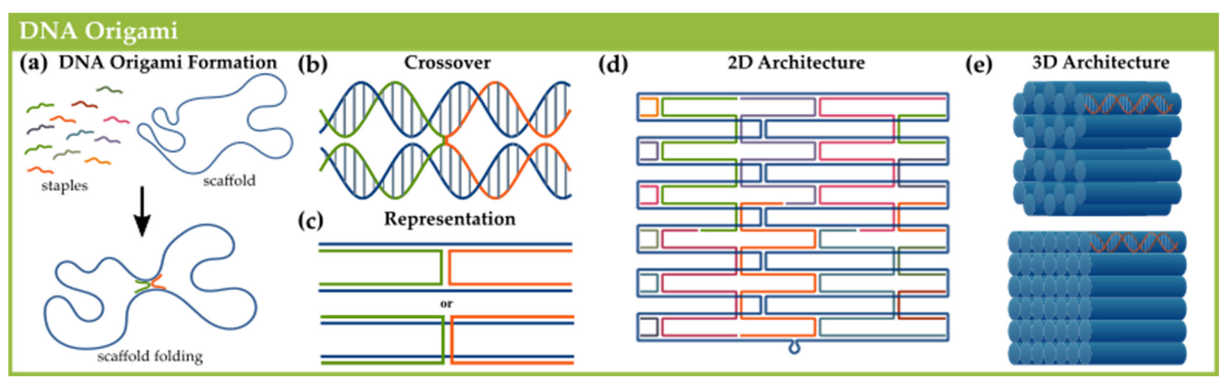
Structural DNA nanotechnology enables the creation of complex polyhedral nanostructures due to the predictability of Watson–Crick base-pairing, wherein adenine (A) and guanine (G) form hydrogen bonds with thymine (T) and cytosine (C) [1,2,3]. Due to the programmable binding of nucleobases, the field of DNA nanotechnology offers an unmatched ability to control the formation of arbitrarily shaped and biocompatible DNA nanostructures [4]. The DNA origami technique is a self-assembly method wherein hundreds of short “staple” oligonucleotides direct the folding of a long single-stranded DNA (ssDNA) “scaffold” to form multilayer and wireframe DNA assemblies (Figure 1) [2,5]. Recently, DNA origami has served to create functional applications such as multifluorophore beacon sensing platforms [6], cargo-sorting robots [7], and drug delivery vehicles [8].
With increasing functional applications, the research community has pioneered innovative tools to facilitate the design process. CaDNAno is a popular computer-aided design (CAD) tool that revolutionized the design process, providing a graphical-user-interface (GUI) and computationally inexpensive method to manually create DNA origami designs from the bottom-up [9]. CaDNAno designs can be built using a square or honeycomb lattice architecture, providing guidance on the available and optimal crossover locations as well as an auto-stapling function. While caDNAno has been so pivotal to the growth of the field, it heavily relies on the expertise of the designer, who must first conceptualize each design before manually implementing the concept. The challenges of manual design can incentivize designers to limit their structures to the simplest geometries. More critically, the manual nature of the process makes it difficult to implement and therefore to compare a range of possible designs to address a given application.
Automated tools have the potential to accelerate the design process and broaden the design space. One powerful approach demonstrated by the tools vHelix [11], DAEDALUS [12], PERDIX [13], and TALOS [14] is the automated generation of nanostructure designs from 3D polyhedral meshes. These tools compute the scaffold routing and staple sequences to create wireframe DNA origami designs from input meshes. MagicDNA is a semi-automated design tool that computes scaffold routing and staple generation from a line model with detailed dimensions of the final design as input [15]. MagicDNA enables an iterative computer-aided engineering (CAE) approach to the design of DNA origami. Thus, current automated tools have enabled automation of key portions of the design process, but they are limited to an approach (top-down) that requires a designer to fully conceptualize the structure. However, it is important to note that the source of the design comes entirely from the user.
Currently, DNA origami design optimization is performed iteratively by human designers, where even veteran designers often get stuck in an infinite iterative design loop in search of the ideal design [16]. Here, we present a novel, formal approach for optimizing the design process for DNA origami through automation. This approach addresses current limitations by computing optimal scaffold routing with only a set of constraints and desired configurations. This is achieved through shape annealing [17], which is an integration of the simulated annealing algorithm, a stochastic optimization technique [18], and shape grammars, which are a formal rule-based generative design method that concisely defines relationships between geometric shapes [19]. Shape annealing generates optimally directed shapes by controlling the selection and implementation of shape transformation rules to evolve a starting shape as the algorithm progresses.
In our first demonstration of this approach, we start with a 3D polyhedral mesh of arbitrary size as input and our algorithm explores the design space to create a variety of unforeseen and legal designs. The 3D polyhedral mesh is merely one example of a constraint, but it is not a requirement for implementing the shape annealing algorithm. This formal approach therefore takes a hybrid top-down and bottom-up direction to nanostructure design. In this work, this approach creates unique routing patterns of the scaffold that, as an initial demonstration in this paper’s implementation, are constrained to the caDNAno honeycomb lattice architecture while designing filling and coating applications. As a note, we refer to “legal” operations as those that are permissible in caDNAno without overriding software recommendations. In this simple demonstration, the shape annealing algorithm enables the automated design of multilayer origami for arbitrary shapes by providing the ability for designers to code for desired features of DNA nanostructures. In this paper we show that shape annealing can be used to design DNA origami by filling or coating polyhedral meshes. The filling application provides a general procedure for filling arbitrary multilayer geometries, while the coating application provides an automated method for creating hollow structures that could be used for casting [20] and cargo-carrying [8] applications.
2. Methods
2.1. Shape Annealing: Optimization with Shape Grammars
The sequencing of constrained DNA strands to meet design goals and constraints is a complex problem, and such layout problems have been shown to have multi-modal and discontinuous spaces [21]. Thus, properties of discrete configuration generation and stochastic search are needed to develop a new algorithm for bottom-up DNA origami design. A method called shape annealing, which was introduced by Cagan and Mitchell [17], utilizes these characteristics.
2.2. Optimization by Simulated Annealing
Shape annealing is a variation of simulated annealing which is a robust and stochastic technique that statistically approaches a global optimum among numerous local optima by accepting worse solutions early on, there-by jumping out of local optima [18]. Simulated annealing (SA), developed by Kirkpatrick et al., can optimize parameters for an arbitrary model and ensure a good solution within sufficient time [18]. SA is a stochastic optimization technique used in many combinatorial optimization problems such as truss design optimization [22] and chip floor planning [23]. The SA algorithm is based on Metropolis’s Monte-Carlo technique, called the Metropolis algorithm [24]. The algorithm randomly samples a feasible solution, , and the energy at that solution, , is calculated. Another random, feasible solution, , is sampled and the energy, , is calculated. In the case of objective minimization, replaces if , or if with a probability, , as a function of temperature, T:
If a generated random number between 0 and 1 is less than , then is accepted; if not, is not replaced. The higher the temperature, the higher the probability of accepting a worse solution. Alternatively, at set temperatures, the higher the difference between the energy states, the lower the probability of accepting worse solutions. The algorithm usually runs for several iterations (or mutations) at a set temperature value until convergence or a set number of iterations (or limit) is reached and then the temperature is reduced. The search process continues until convergence or equilibrium is reached, or the temperature reaches zero. The algorithm is analogous to the annealing process of metals, where the energy can be substituted for an objective function and the temperature is a multiplier that adjusts the probability of accepting a worse solution that dynamically changes as the algorithm runs. An appropriate cooling schedule must be chosen to reduce the temperature. Although a specific cooling schedule that theoretically satisfies convergence is one that follows a logarithmic trend, it would exponentially increase the search time for larger problems. The current work uses a geometric cooling schedule that follows an exponential trend:
where is between 0 and 1. Although this schedule does not guarantee convergence to the global optimum, it searches for a good solution in sufficient time. The temperature continues to be reduced, with the algorithm running for several iterations per temperature, until a temperature of zero is reached. It is important to note that there are “adaptive” annealing schedules that adjust the temperature reduction based on local performance [25,26]. However, for DNA origami applications in this work, the simple geometric schedule performs sufficiently well.
2.3. Shape Grammars
Simulated annealing requires neighborhood moves for each variation, which is the replacement of the current solution by the test solution. Shape annealing utilizes simulated annealing to control the search process and defines the move set through a formal language of shape known as shape grammars. Shape grammars, introduced by Stiny, provides an effective way to concisely encode knowledge of how to legally assemble various artifact forms together through a set of shape transformation rules that are applied iteratively from a starting shape to generate a different, evolving shape [19]. These geometric shapes are typically 2D or 3D. Spatial transformations of translation, rotation, reflection, and scale, and boolean operations of union, intersection, and subtraction can be achieved using shape grammars. Generally, each shape transformation rule specifies a condition and an associated action. In addition to defining a language of form, shape grammars have been utilized for functional designs such as MEMS resonators [27] and roof trusses [28]. Thus, with shape annealing, geometric forms are generated based on the language of a shape grammar to fulfill goals and constraints through stochastic search.
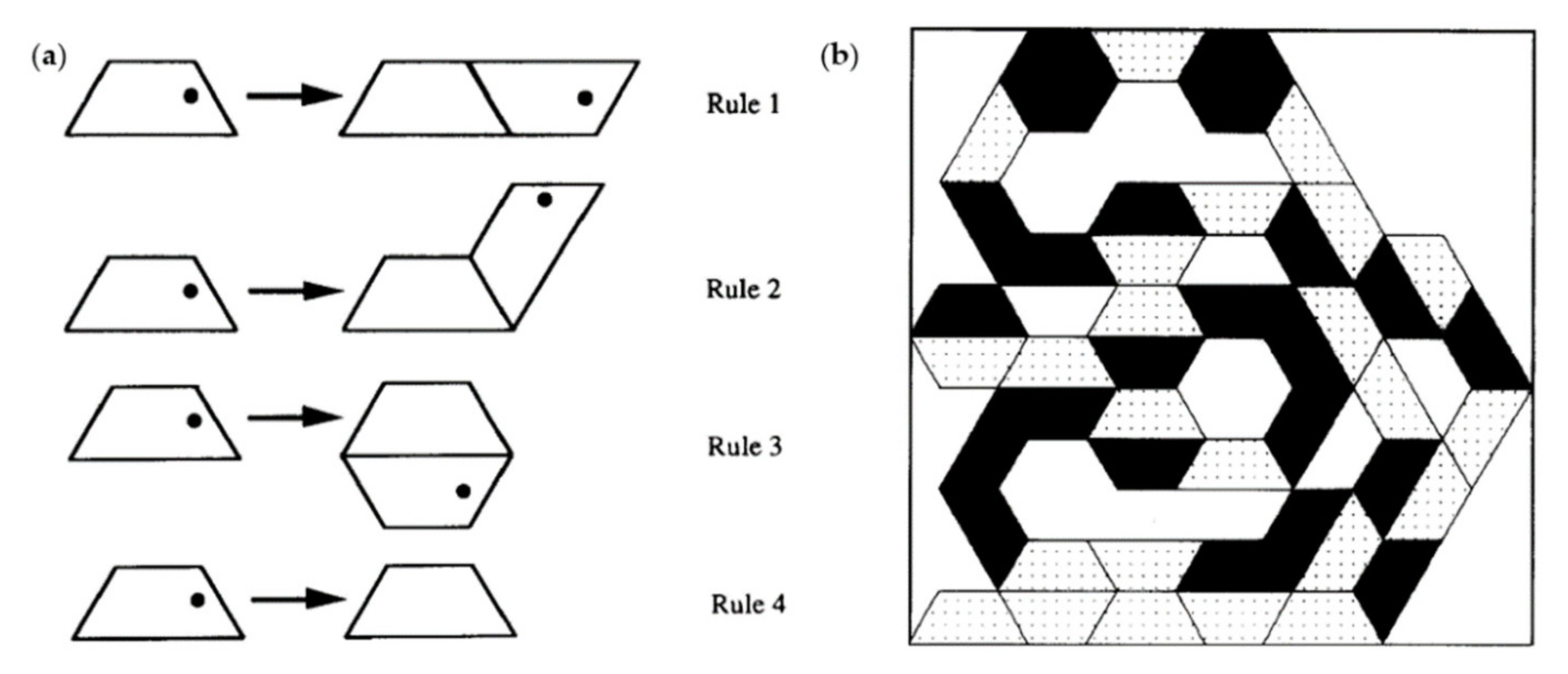
In the original introduction of shape annealing, a snake-like grammar was defined to pack a 2D volume (Figure 2). The insight of this paper is that the sequencing of DNA has a similar snake-like property. As such, in this work, we introduce the shape annealing methods for the design of DNA origami, providing a new generative CAD hybrid top-down and bottom-up approach that results in novel DNA sequences that fulfill a functional need without requiring a prior configuration, or envisioning of the solution.
Since DNA origami is fundamentally based on the path of the scaffold that is then cinched with staple strands, the shape grammars in Figure 3 encode knowledge of how to legally assemble a continuous scaffold strand constrained to the caDNAno honeycomb lattice architecture. The grammar ensures legal designs by incorporating the dimensions of a double-stranded DNA (dsDNA) with a helical diameter of 2 nm cut into an axial length of 2.38 nm (axial rise of 0.34 nm per base). According to the mathematics of the honeycomb lattice architecture, 7 bases is approximately 240 degrees. Therefore, a central helix can address all three nearest neighbors along its length by placing crossovers at multiples of 7 base pairs [5,9].
The shape grammar for the generated designs generalizes the scaffold into short helical 7 base pair (bp) segments with physical dimensions of the dsDNA double helix, where potential crossovers are located at the start and end of the segment. The grammar further represents short helical segments running clockwise in the −z direction as blue, and segments running counterclockwise in the +z direction as red. The nearest neighbors of the blue and red helices are at a −180° angle difference, where potential crossovers for the blue helix are in the order of 0°, 120°, and 240°. The arrow labels indicate the potential crossover locations and therefore where a rule can be applied along the helix. The grammar consists of two addition rules, which allow scaffold growth based on the honeycomb lattice constraint, and a reversal rule, which removes a segment for both additive rules. Although there are several possible crossover locations along the scaffold, for simplicity, the grammar restricts this to the three positions which provide nearest neighbor crossover positions for the honeycomb lattice. This restriction, which generates legal honeycomb designs, can, however, be relaxed in the future to create more complex lattice designs such as hybrid square and honeycomb architectures.
2.4. Shape Annealing
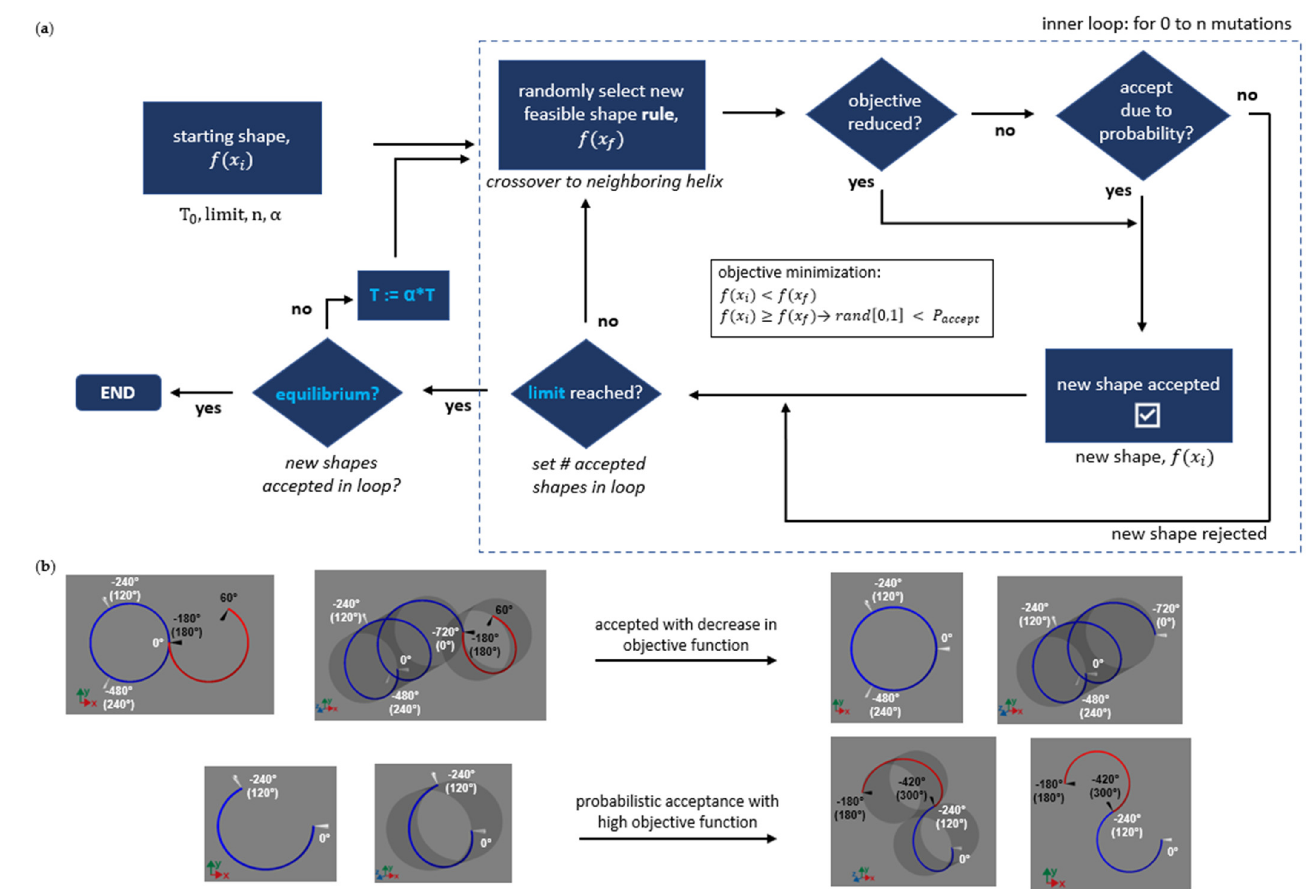
Shape annealing utilizes the simulated annealing algorithm to control the application of randomly selected shape rules at a given state. The pseudocode in Algorithm 1 provides a more detailed description of how the shape annealing algorithm works. Figure 4 illustrates examples of the shape annealing algorithm for scaffold routing when constrained to a honeycomb lattice architecture. A feasible shape rule is selected from the language and applied to the current design state. If the new design complies with the defined constraints, it is sent to the Metropolis algorithm, where the new state is compared to the old state. If the new state complies with the desired design features, it is accepted; if not, the old state is retained. In this current work, the grammar has a reversal rule (Figure 3c) applied to rules 1 and 2 (Figure 3a,b) to prevent rapid convergence on an inferior solution by enabling the algorithm to back out of local solutions. The rules in Figure 3 define the design space used to create DNA origami designs consisting of a continuous scaffold strand.
In the shape annealing algorithm, the number of outer loop iterations, which is determined by the reduction factor (α), the number of inner loop iterations, which is the mutations (n), the initial temperature before the algorithm proceeds (T), and the limit, which is the number of accepted shapes within the inner loop, must be determined to ensure convergence on good solutions. By adjusting these key parameters, the shape annealing algorithm will generate unique shapes. Figure 4a displays a generic flowchart of the shape annealing algorithm, while Figure 4b displays examples of rule applications with objective function calculations.
| Algorithm 1 Shape annealing algorithm | |
| 1: | initialize T, limit, n, α |
| 2: | generate initial_shape |
| 3: | state = evaluate(initial_shape) |
| 4: | procedure Shape Anneal(state, T, limit, n, α) t→ key parameters |
| 5: | while T > 0 do |
| 6: | success=0, i =0 |
| 7: | for i to n do t→ mutations=n |
| 8: | prev_state=state |
| 9: | new_shape=random_rule() |
| 10: | if new_shape complies with constraints then |
| 11: | new_state=evaluate(new_shape) |
| 12: | test = metropolis(new_state, prev_state, T) |
| 13: | if test then |
| 14: | state=new_state |
| 15: | success += 1 |
| 16: | end if |
| 17: | end if |
| 18: | if success>limit then |
| 19: | break |
| 20: | end if |
| 21: | end for |
| 22: | if success=0 then t→ equilibrium |
| 23: | break |
| 24: | end if |
| 25: | T = T*α |
| 26: | end while |
| 27: | end procedure |
2.5. Coarse-Grain Simulations
OxDNA is a coarse-grain nucleotide-level DNA model that has proven to be exceptionally apt at capturing the structural, mechanical, and thermodynamic properties of DNA [30,31]. As an extension, oxDNA can realistically model the properties of larger DNA origami structures and is widely used to study such systems [32,33,34,35]. Due to this ability to model DNA origami structures and to correctly predict stability and structural configuration, oxDNA simulations are used in this study to evaluate the validity of generated structures. In addition, simulations provide the ability to analyze the resulting structure with much greater detail than possible through experimental imaging approaches. In this study, simulations of the generated designs follow a very typical relaxation approach that is outlined by Doye et al. consisting of a minimization step, in which overlapping nucleotide volumes are resolved, followed by a relaxation step, in which overextended bonds are resolved and the structures are allowed to take on a relaxed configuration [36]. The relaxation step for these simulations run for 106 steps once final designs are derived. This 2-step relaxation sequence is followed by a 106 step regular molecular dynamics simulation with no added forces or modified potentials used for root mean-square fluctuations (RMSF) calculations. All simulations are carried out at room temperature (295 K) with a 15.15 fs time step (0.005 in simulation units) with all other parameters following the recommendations outlined by Doye et al. [36].
3. Applications
With arbitrary 3D triangular meshes as input, our shape annealing platform generates filled or coated structures. While there are automated tools for converting triangular meshes into DNA origami designs, these tools are limited to wireframe structures [11,12,13,14]. In this paper, the shape annealing framework imports three distinct triangular meshes as input for the generation of filled and coated multilayer DNA origami designs. After the shapes are generated with their respective filling or coating algorithm, they are converted to caDNAno JSON files using a custom scadnano Python script [37] and then auto-stapled using the caDNAno auto-stapling function. After auto-stapling, the caDNAno JSON files are converted to PDB files using TacoxDNA for visualization [38]. After visualization, the caDNAno JSON files are then converted to oxDNA topology and configuration files using TacoxDNA. The oxDNA topology and configuration files are then imported to oxDNA to evaluate structural validation. The results from oxDNA are analyzed using the RMSF scripts and visualized in oxView, which are both developed by Poppleton et al. [39]. The last frame of the oxDNA simulation is then converted to PDB using TacoxDNA.
3.1. Filling Application
The filling application presents a simple demonstration of the shape annealing algorithm. It is particularly useful for generating solid designs under conditions of complex bounding shapes because segments can only be generated within the confines of a defined geometry. One of the metrics defined to evaluate the filling of an arbitrary geometry is packing density, where the goal is to maximize the number of helices within the geometry. Once these arbitrary geometries become more complex, path direction should be incorporated, where the helices grow towards the surface and thus the corners of the geometry. The filling application accounts for this by presenting an optimization problem with the goal of minimizing the distance of the helical segments to the inner surface of the mesh to generate a scaffold of custom length within an arbitrary geometry. The scaffold, in 7 bp segments, is assembled based on the shape grammars where no segments can overlap, the generated segment must fit within the bounds of the defined space, and the shapes are generated to imitate continuous scaffold length growth. The filling application presents the case of objective minimization, where replaces if , or if , with a probability. The objective function is an exponential function:
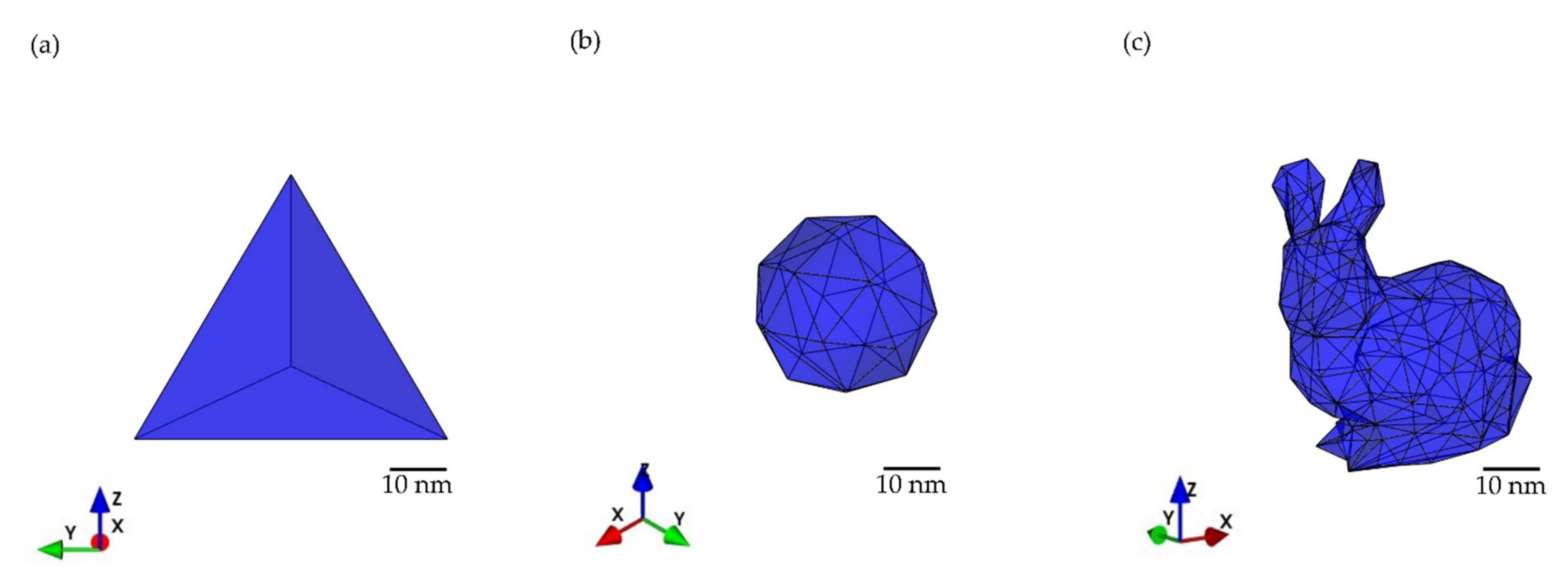
where x is the Euclidian distance from the inner surface of the mesh to the top of each helical segment. This objective function was selected since it exponentially decreases distances near the surface of the polyhedral mesh. An objective function with a base value much greater than one acts more like a step-function and is too restrictive. However, an objective function with a base value only slightly greater than one is not as restrictive. Thus, 1.12 is an appropriate base value for this function. As a demonstration of the method’s capability to fill input triangular meshes, we present three examples of the filling application using a tetrahedron, a snub cuboctahedron (snub cube), and a version of the Stanford bunny (Figure 5).
3.2. Coating Application
Due to its complexity and rigidity, DNA nanostructures can be used as a template to assemble inorganic materials in defined patterns [40]. Sun et al. illustrated the design of DNA into mechanically stiff molds to cast and synthesize metallic nanoparticles into desired 3D configurations [20]. These 3D molds, originally designed through caDNAno, encapsulate a nucleating gold seed that grows to fill up the entire volume, thus reproducing its 3D shape. Although the wireframe design tools automate the design of rigid wireframe-based DNA nanostructures, current approaches have limited options for controlling the mechanical properties of automated structures. A multilayer DNA origami approach, as noted by Sun et al., provides broad control over the mechanical properties of the mold, which are critical to casting applications [20]. However, even though our framework was developed to promote filling, it can be applied to coat the surface of arbitrary geometries with a scaffold of custom length to create solid DNA molds; thus, providing the automated generation of multilayer DNA origami based on 3D polyhedral meshes. The optimization problem in this example minimizes the distance of helical segments to the outer surface of the input mesh. The scaffold, in 7 bp segments, is assembled based on the shape grammars where no segments can overlap, and the shapes are generated to imitate continuous scaffold length growth. The coating application presents the case of objective minimization (Section 2.2). The objective function is:
where x is the Euclidean distance from the outer surface of the mesh to the top of each helical segment. The objective function finds the minimum perpendicular distance to the surface of the mesh. This objective function was selected because it gradually decreases distances closer to the outer surface of the polyhedral mesh. An objective function with a base value much closer to one generates designs that are not as tightly coated. However, an objective function with a base value close to two generates designs that tightly coats the surface of the mesh. Thus, 1.19 is an appropriate base value for this function. As a demonstration of the method’s capability to coat the surface of input meshes, we present three examples of the coating application using a tetrahedron, a snub cube, and a version of the Stanford bunny (Table 1).
4. Results
As the simulated annealing algorithm can converge to a local minimum due to its stochastic nature, the algorithm is typically run several times and the best generated solution is selected [23]. In this work the algorithm is run in sets of 10, with the best solution of each set presented as the selected solution. Here, the filling and coating algorithms are run in 10 batches of 10 (100 times total per mesh) where the best generated shape is selected per batch, resulting in 10 best shapes out of 100 that are evaluated as the goodness of the algorithm. Since the metric of success for the filling application is packing density, 10 shapes with the highest number of helical segments per batch are selected. Table 2 illustrates the mean and standard deviation of the total number of helical segments over the 100 runs and the 10 top runs per batch for the filling application. For the coating application, the metric of success is how tightly the scaffold wraps around the mesh. Currently, the tightness is assessed by selecting designs with a higher number of helical segments close to the mesh. Table 3 illustrates the mean and standard deviation of the total number of helical segments close to the mesh over the 100 runs and the 10 top runs per batch for the coating application. Figure 6 illustrates three out of 10 of the best shapes generated with the shape annealing algorithm per input mesh for the filling application. The shapes generated from the filling application share the same optimization parameters; this is also the same for the coating application (Table 4). Figure 7 illustrates the relaxed configurations for the filling application after structural validation through oxDNA. Figure 8 illustrates the root mean-square fluctuations (RMSF) of the structures generated from oxDNA for the filling application with the total energy over the course of the relaxation simulation plotted in Figure 9. Figure 10 illustrates three out of 10 of the best shapes generated with the shape annealing algorithm per input mesh for the coating application. Figure 11, Figure 12 and Figure 13 provide a visualization of how the scaffold grows during the annealing schedule for the filling application, which are generated through Mayavi, a 3D visualization Python package [41]. The total number of iterations until convergence per mesh is divided equally into 50 steps and an image is generated at every step.
5. Discussion
Figure 6 shows that the proposed framework is capable of filling arbitrary shapes, particularly complex geometries such as the Stanford bunny, with high range of possible scaffold designs. The helical segments were able to reach the ears of the Stanford bunny, which are much further from the center of mass. Therefore, a larger design space lets the algorithm explore deeper corners of complex structures with the scaffold, even within constricted spaces whose narrowest dimensions are only two or three times as large as the diameter of dsDNA. The filling application is also able to replicate the shape of the tetrahedron and snub cube, with sharp and soft corners, respectively. The shape generated from the tetrahedron clearly demonstrates that the filling application can generate solid DNA origami designs with varying cross-sections. As observed in Table 2 for the filling application, the total number of helical segments averaged over all 100 iterations is lower than the average of the 10 top results. While the standard deviation of the total number of helical segments over all 100 iterations is much higher than the standard deviation for the 10 top results. Due to the stochastic nature of the algorithm, there is high variation among consecutive runs, as the algorithm can still get stuck in a local optimum near the global optimum. However, the best solutions are more tightly converged to a higher quality, even though the topology still varies.
One way to drive coating behavior is to incentivize the minimization of the distance of helical segments to the surface of a polyhedral mesh through the objective function. Figure 10 illustrates the coating of different polyhedral meshes, and this demonstrates the adaptability of the shape annealing algorithm in formalizing different types of constraints. This application is the first step to realizing the articulation of a variety of desired features. While the current coating application generates designs with limited coverage, alternative objective functions could lead to better coating. In Table 3, the number of helical segments close to the mesh averaged over all 100 iterations is much lower than the 10 top results. While the standard deviation over all 100 iterations of the number of helical segments close to the mesh is much higher than the 10 top results. Figure 10 illustrates the stochastic nature of the scaffold routing pattern, which does not conform to the typical routing of a human designer where there is typically a seam near the middle of the 2D drawing, as seen in Figure 1d.
Figure 11, Figure 12 and Figure 13 illustrate how the shapes generated by the shape annealing algorithm evolve into their final configuration. As illustrated in the higher iteration numbers in Figure 11, Figure 12 and Figure 13, as the shape annealing algorithm approaches equilibrium, fewer shape rules with worse solutions are accepted. As observed, the final configuration is highly dependent on the initial path generated and tweaking the shape annealing parameters, which pose as the serial number for each application, changes the characteristics of the final shape (Table 3). At the start of the schedule, most generated configurations are better than the previous, thus most new shapes are accepted. If an appropriate initial path is not generated, the algorithm will not be able to effectively coat or fill a geometry, resulting in the large range of solutions per batch.
Simulation results for all structures are depicted in Figure 7, Figure 8 and Figure 9. It is clear from the observed plateauing of the energy in Figure 9 that the relaxation simulation length is more than appropriate. This is not surprising as the structures require minimal component translation or rotation to reach a relaxed state from their initial conformation. The most common deviations from the intended shapes seen in the final relaxed conformations are fraying strands that occur at the surfaces of the structures. This fraying occurs across all generated structures and, in general, is a result of a lack of sufficient crossovers required to hold the strands together within these regions. This similarly explains other events where a lack of sufficient crossovers results in a fracture or similar structural failures, such as the fracture that can be seen in Figure 7c. Structural errors due to low local crossover densities are more likely to occur in regions with reduced number of neighboring helixes and in regions with reduced helical lengths. In other words, they are more likely to occur in regions with a reduced number of possible crossover positions. Therefore, surface fraying events are more likely to occur than fractures and fractures are more likely to occur at points of reduced cross-sectional area. Thus, small details, such as the ears of the Stanford bunny or the corners of a tetrahedron, which have both traits, are particularly likely to unfold. However, it should be emphasized that this issue is not exclusive to these generated shapes, as a low number of possible crossover positions make it difficult create structurally sound small details within a structure regardless of design approach. The filled structures largely maintain their intended shape and, due to the high stability of the honeycomb lattice, they experience no noticeable twist or large deformations in solid regions. Furthermore, given the relatively low time and monetary requirements to characterize structures using simulations, designs with significant fraying or major structural defects can be quickly detected and discarded. RMSF data for the structures remains largely unsurprising. There appears to be a general increase of RMSF magnitude towards the outer edges of the structure that is characteristic of DNA structures due to the inherent flexibility of the material and the decrease in structural support towards the surfaces. RMSF values are also maximum for the frayed strands which can be characterized as undergoing mostly free Brownian motion.
Future work will focus on how to better articulate the algorithm for coating arbitrary geometries. It would be interesting to apply more constraints, such as an outer mesh, for the coating application in order to automate the scaffold routing of DNA origami molds with tunable and uniform thickness. We will also explore other objective functions or constraints to address long standing challenges in the field of DNA origami design, such as limited knowledge in design-property relationships to decrease the design-iteration loop, increase design stability, and increase the yield in DNA origami nanostructures [16]. For example, Ke et al. developed design rules empirically to increase the yield in multilayer DNA origami assemblies, which could be incorporated into our shape annealing platform in the future [42]. In addition to addressing long-standing challenges in the field of DNA origami design, since our current work considers the scaffold as linear, it would be interesting to unite the beginning and end of the scaffold to generate a circular strand from the algorithm. Furthermore, since the optimization of scaffold growth for desired features can be applied to other methods, areas of future work also include exploring other algorithms to better achieve desired goals. For example, Yogov et al. applied the genetic algorithm [43], which mimics biological evolution, to the design of continuous 3D load-supporting structures to achieve desired goals [44].
6. Conclusions
We have introduced shape annealing as a robust method to control the generation of helical segments. Using shape grammars based on optimally directed scaffold patterns, we demonstrate a filling and coating application. This formal approach addresses the limitations of top-down automated design through shape grammars coupled with optimization strategies. It performs parameterized design to conceptualize multilayer DNA origami designs of complex bounding geometries. By exploiting DNA’s predictable and programmable characteristics, the scaffold can be routed in unpredictable ways through automation, which significantly expands the design space that can be considered.
Author Contributions
Conceptualization, J.C. and R.E.T.; methodology, J.C. and R.E.T.; validation, D.S.A.; investigation, B.B.; resources, J.C. and R.E.T.; data curation, B.B.; writing—review and editing, B.B., D.S.A., J.C. and R.E.T.; visualization, B.B. and R.E.T.; supervision, J.C. and R.E.T. All authors have read and agreed to the published version of the manuscript.
Funding
This research was funded by the Air Force Office of Scientific Research (AFOSR) Young Investigator Research Program (YIP) award through grant FA9550-18-1-0199, the Air Force Office of Scientific Research through grant FA9550-18-0088, and the Defense Advanced Research Projects Agency through cooperative agreement No. N66001-17-1-4064. Any opinions, findings, and conclusions or recommendations expressed in this material are those of the authors and do not necessarily reflect the views of the sponsors.
Institutional Review Board Statement
Not applicable.
Conflicts of Interest
The authors declare no conflict of interest.
References
- Seeman, N.C. Nucleic Acid Junctions and Lattices. J. Theor. Biol. 1982, 99, 237–247. [Google Scholar] [CrossRef]
- Rothemund, P.W.K. Folding DNA to Create Nanoscale Shapes and Patterns. Nature 2006, 440, 297–302. [Google Scholar] [CrossRef] [Green Version]
- Seeman, N.C.; Sleiman, H.F. DNA Nanotechnology. Nat. Rev. Mater. 2017, 3, 1–23. [Google Scholar] [CrossRef]
- Tørring, T.; Gothelf, K.V. DNA Nanotechnology: A Curiosity or a Promising Technology? F1000Prime Rep. 2013, 5, 14. [Google Scholar] [CrossRef] [PubMed] [Green Version]
- Castro, C.E.; Kilchherr, F.; Kim, D.-N.; Shiao, E.L.; Wauer, T.; Wortmann, P.; Bathe, M.; Dietz, H. A Primer to Scaffolded DNA Origami. Nat. Methods 2011, 8, 221–229. [Google Scholar] [CrossRef] [PubMed]
- Selnihhin, D.; Sparvath, S.M.; Preus, S.; Birkedal, V.; Andersen, E.S. Multifluorophore DNA Origami Beacon as a Biosensing Platform. ACS Nano 2018, 12, 5699–5708. [Google Scholar] [CrossRef]
- Thubagere, A.J.; Li, W.; Johnson, R.F.; Chen, Z.; Doroudi, S.; Lee, Y.L.; Izatt, G.; Wittman, S.; Srinivas, N.; Woods, D.; et al. A Cargo-Sorting DNA Robot. Science 2017, 357, eaan6558. [Google Scholar] [CrossRef] [Green Version]
- Douglas, S.M.; Bachelet, I.; Church, G.M. A Logic-Gated Nanorobot for Targeted Transport of Molecular Payloads. Science 2012, 335, 831–834. [Google Scholar] [CrossRef]
- Douglas, S.M.; Marblestone, A.H.; Teerapittayanon, S.; Vazquez, A.; Church, G.M.; Shih, W.M. Rapid Prototyping of 3D DNA-Origami Shapes with CaDNAno. Nucleic Acids Res. 2009, 37, 5001–5006. [Google Scholar] [CrossRef] [PubMed] [Green Version]
- Wang, W.; Arias, D.S.; Deserno, M.; Ren, X.; Taylor, R.E. Emerging Applications at the Interface of DNA Nanotechnology and Cellular Membranes: Perspectives from Biology, Engineering, and Physics. APL Bioeng. 2020, 4, 041507. [Google Scholar] [CrossRef] [PubMed]
- Benson, E.; Mohammed, A.; Gardell, J.; Masich, S.; Czeizler, E.; Orponen, P.; Högberg, B. DNA Rendering of Polyhedral Meshes at the Nanoscale. Nature 2015, 523, 441–444. [Google Scholar] [CrossRef] [PubMed] [Green Version]
- Veneziano, R.; Ratanalert, S.; Zhang, K.; Zhang, F.; Yan, H.; Chiu, W.; Bathe, M. Designer Nanoscale DNA Assemblies Programmed from the Top Down. Science 2016, 352, 1534. [Google Scholar] [CrossRef] [PubMed] [Green Version]
- Jun, H.; Zhang, F.; Shepherd, T.; Ratanalert, S.; Qi, X.; Yan, H.; Bathe, M. Autonomously Designed Free-Form 2D DNA Origami. Sci. Adv. 2019, 5, eaav0655. [Google Scholar] [CrossRef] [PubMed] [Green Version]
- Jun, H.; Shepherd, T.R.; Zhang, K.; Bricker, W.P.; Li, S.; Chiu, W.; Bathe, M. Automated Sequence Design of 3D Polyhedral Wireframe DNA Origami with Honeycomb Edges. ACS Nano 2019, 13, 2083–2093. [Google Scholar] [CrossRef] [PubMed]
- Huang, C.-M.; Kucinic, A.; Johnson, J.A.; Su, H.-J.; Castro, C.E. Integrating Computer-Aided Engineering and Computer-Aided Design for DNA Assemblies. bioRxiv 2020. [Google Scholar] [CrossRef]
- Majikes, J.M.; Liddle, J.A. DNA Origami Design: A How-To Tutorial. J. Res. Natl. Inst. Stan. 2020, 126, 126001. [Google Scholar] [CrossRef]
- Cagan, J.; Mitchell, W.J. Optimally Directed Shape Generation by Shape Annealing. Environ. Plan. B 1993, 20, 5–12. [Google Scholar] [CrossRef]
- Kirkpatrick, S.; Gelatt, C.D.; Vecchi, M.P. Optimization by Simulated Annealing. Science 1983, 220, 671–680. [Google Scholar] [CrossRef]
- Stiny, G. Introduction to Shape and Shape Grammars. Environ. Plan. B 1980, 7, 343–351. [Google Scholar] [CrossRef] [Green Version]
- Sun, W.; Boulais, E.; Hakobyan, Y.; Wang, W.L.; Guan, A.; Bathe, M.; Yin, P. Casting Inorganic Structures with DNA Molds. Science 2014, 346, 1258361. [Google Scholar] [CrossRef] [Green Version]
- Cagan, J.; Shimada, K.; Yin, S. A Survey of Computational Approaches to Three-Dimensional Layout Problems. Comput. Aided Des. 2002, 34, 597–611. [Google Scholar] [CrossRef] [Green Version]
- Elperin, T. Monte Carlo Structural Optimization in Discrete Variables with Annealing Algorithm. Int. J. Numer. Methods Eng. 1988, 26, 815–821. [Google Scholar] [CrossRef]
- Rutenbar, R.A. Simulated Annealing Algorithms: An Overview. IEEE Circuits Devices Mag. 1989, 5, 19–26. [Google Scholar] [CrossRef]
- Metropolis, N.; Rosenbluth, A.W.; Rosenbluth, M.N.; Teller, A.H.; Teller, E. Equation of State Calculations by Fast Computing Machines. J. Chem. Phys. 1953, 21, 1087–1092. [Google Scholar] [CrossRef] [Green Version]
- Huang, M.D.; Romeo, F.; Sangiovanni-Vincentelli, A.S. An Efficient General Cooling Schedule for Simulated Annealing. In Proceedings of the IEEE International Conference on Computer-Aided Design, Santa Clara, CA, USA, 10–13 November 1986; pp. 381–384. [Google Scholar]
- Triki, E.; Collette, Y.; Siarry, P. A Theoretical Study on the Behavior of Simulated Annealing Leading to a New Cooling Schedule. Eur. J. Oper. Res. 2005, 166, 77–92. [Google Scholar] [CrossRef]
- Agarwal, M.; Cagan, J.; Stiny, G. A Micro Language: Generating MEMS Resonators by Using a Coupled Form—Function Shape Grammar. Environ. Plan. B Plan. Des. 2000, 27, 615–626. [Google Scholar] [CrossRef]
- Shea, K.; Cagan, J. Languages and Semantics of Grammatical Discrete Structures. Artif. Intell. Eng. Des. Anal. Manuf. 1999, 13, 241–251. [Google Scholar] [CrossRef] [Green Version]
- Cagan, J. Shape Annealing Solution to the Constrained Geometric Knapsack Problem. Comput. Aided Des. 1994, 26, 763–770. [Google Scholar] [CrossRef]
- Šulc, P.; Romano, F.; Ouldridge, T.E.; Rovigatti, L.; Doye, J.P.K.; Louis, A.A. Sequence-Dependent Thermodynamics of a Coarse-Grained DNA Model. J. Chem. Phys. 2012, 137, 135101. [Google Scholar] [CrossRef]
- Ouldridge, T.E.; Louis, A.A.; Doye, J.P.K. Structural, Mechanical, and Thermodynamic Properties of a Coarse-Grained DNA Model. J. Chem. Phys. 2011, 134, 085101. [Google Scholar] [CrossRef] [Green Version]
- Engel, M.C.; Smith, D.M.; Jobst, M.A.; Sajfutdinow, M.; Liedl, T.; Romano, F.; Rovigatti, L.; Louis, A.A.; Doye, J.P.K. Force-Induced Unravelling of DNA Origami. ACS Nano 2018, 12, 6734–6747. [Google Scholar] [CrossRef]
- Huang, C.-M.; Kucinic, A.; Le, J.V.; Castro, C.E.; Su, H.-J. Uncertainty Quantification of a DNA Origami Mechanism Using a Coarse-Grained Model and Kinematic Variance Analysis. Nanoscale 2019, 11, 1647–1660. [Google Scholar] [CrossRef] [PubMed]
- Snodin, B.E.K.; Schreck, J.S.; Romano, F.; Louis, A.A.; Doye, J.P.K. Coarse-Grained Modelling of the Structural Properties of DNA Origami. Nucleic Acids Res. 2019, 47, 1585–1597. [Google Scholar] [CrossRef] [Green Version]
- Suma, A.; Stopar, A.; Nicholson, A.W.; Castronovo, M.; Carnevale, V. Global and Local Mechanical Properties Control Endonuclease Reactivity of a DNA Origami Nanostructure. Nucleic Acids Res. 2020, 48, 4672–4680. [Google Scholar] [CrossRef] [PubMed] [Green Version]
- Doye, J.P.K.; Fowler, H.; Prešern, D.; Bohlin, J.; Rovigatti, L.; Romano, F.; Šulc, P.; Wong, C.K.; Louis, A.A.; Schreck, J.S.; et al. The OxDNA Coarse-Grained Model as a Tool to Simulate DNA Origami. arXiv 2020, arXiv:2004.05052. [Google Scholar]
- Doty, D.; Lee, B.L.; Stérin, T. Scadnano: A Browser-Based, Scriptable Tool for Designing DNA Nanostructures. arXiv 2020, arXiv:2005.11841. [Google Scholar]
- Suma, A.; Poppleton, E.; Matthies, M.; Šulc, P.; Romano, F.; Louis, A.A.; Doye, J.P.K.; Micheletti, C.; Rovigatti, L. TacoxDNA: A User-Friendly Web Server for Simulations of Complex DNA Structures, from Single Strands to Origami. J. Comput. Chem. 2019, 40, 2586–2595. [Google Scholar] [CrossRef]
- Poppleton, E.; Bohlin, J.; Matthies, M.; Sharma, S.; Zhang, F.; Šulc, P. Design, Optimization and Analysis of Large DNA and RNA Nanostructures through Interactive Visualization, Editing and Molecular Simulation. Nucleic Acids Res. 2020, 48, e72. [Google Scholar] [CrossRef]
- Bayrak, T.; Helmi, S.; Ye, J.; Kauert, D.; Kelling, J.; Schönherr, T.; Weichelt, R.; Erbe, A.; Seidel, R. DNA-Mold Templated Assembly of Conductive Gold Nanowires. Nano Lett. 2018, 18, 2116–2123. [Google Scholar] [CrossRef]
- Ramachandran, P.; Varoquaux, G. Mayavi: 3D Visualization of Scientific Data. Comput. Sci. Eng. 2011, 13, 40–51. [Google Scholar] [CrossRef] [Green Version]
- Ke, Y.; Bellot, G.; Voigt, N.V.; Fradkov, E.; Shih, W.M. Two Design Strategies for Enhancement of Multilayer–DNA-Origami Folding: Underwinding for Specific Intercalator Rescue and Staple-Break Positioning. Chem. Sci. 2012, 3, 2587–2597. [Google Scholar] [CrossRef] [PubMed] [Green Version]
- Holland, J.H. Adaptation in Natural and Artificial Systems: An Introductory Analysis with Applications to Biology, Control, and Artificial Intelligence; MIT Press: Cambridge, MA, USA, 1992; ISBN 978-0-262-27555-2. [Google Scholar]
- Yogev, O.; Shapiro, A.A.; Antonsson, E.K. Computational Evolutionary Embryogeny. Trans. Evol. Comp. 2010, 14, 301–325. [Google Scholar] [CrossRef] [Green Version]
Figure 1.
DNA origami folding method: (a) DNA origami nanostructures are assembled from the directed folding of the scaffold strand (blue) by staple strands (multicolored); (b) Individual helical domains are connected by interhelix crossovers; (c) These interhelix crossovers are represented as straight vertical segments; (d) CaDNAno editing is done using a simple 2D visualization of a DNA origami nanostructure that folds into a 3D model; (e) These 3D DNA origami models represent the DNA double helix as a solid cylinder and generally follow a honeycomb (top) or square (bottom) lattice architecture (adapted from Wang et al. [10]).

Figure 2.
Snake-like shape grammars of half-hexagons: (a) Four simple shape grammar rules consisting of half-hexagons with a long base of one unit and a short base of one-half unit. Rule 4 is created to complete the final generated shape; (b) Final generated shape based on the snake-like shape grammar constrained to a 5 × 5 unit box with the condition of no pieces overlapping. The fill pattern indicated the applied rule, where a light fill points to rule 1, a medium fill points to rule 2 and a dense fill points to rule 3 (adapted from Cagan [29]).

Figure 3.
Shape grammar example for scaffold routing when constrained to a honeycomb lattice architecture. The scaffold is sectioned into 7-base helical segments with the physical dimension of the dsDNA right-handed double helix. The blue helix segment is directed in the −z direction (5′ end to 3′ end) while the red helix segment is directed in the +z direction (3′ end to 5′ end): (a) Rule 1 is for generating helix segments that crossover to a neighboring helix (0°, 120°, and 240° for the blue helix, in order; −180°, 60°, and 300° for the red helix, in order). Illustrated is a crossover at 120° from the blue helix segment; (b) Rule 2 is for extending the helix by a segment. Illustrated is an extension at 120° from the blue helix segment to create a longer helix ending at 240°; (c) Rule 3 is for removing a 7-base helical segment to prevent rapid convergence on an inferior solution. Illustrated is an example of rule 3, which here is the reversal of rule 1 by removing the red helix segment at 300° which leaves the blue helix segment ending at 240°.

Figure 4.
Shape annealing algorithm for scaffold routing when constrained to a honeycomb lattice architecture. Key steps are initializing the temperature, verifying desired goal with metropolis function, checking whether the limit and equilibrium has been reached, and reducing the temperature. Key parameters are the temperature (T), mutations (n), limit, and reduction factor (α): (a) General flowchart of the shape annealing algorithm.; (b) Two examples of rule applications based on objective minimization. The top example shows the shape rule 3 (reversal rule) accepted with a decrease in objective function. The bottom example shows the shape rule 1 (additive rule) accepted with a probability due to an increase in objective function.

Figure 5.
Input triangular mesh with a scale bar of 10 nm in length: (a) Tetrahedron mesh with dimensions for the filling application of the axis aligned bounding box of 47.6 nm in length, 55.0 nm in width, and 45.9 nm in height. This mesh has a volume of 19,600 ; (b) Snub cuboctahedron mesh with the axis aligned bounding box of 35.1 nm in length, 36.0 nm in width, and 35.8 nm in height. This mesh has a volume of 20,000 ; (c) Stanford bunny mesh with the axis aligned bounding box of 54.1 nm in length, 43.3 nm in width, and 53.6 nm in height. This mesh has a volume of 34,200 .

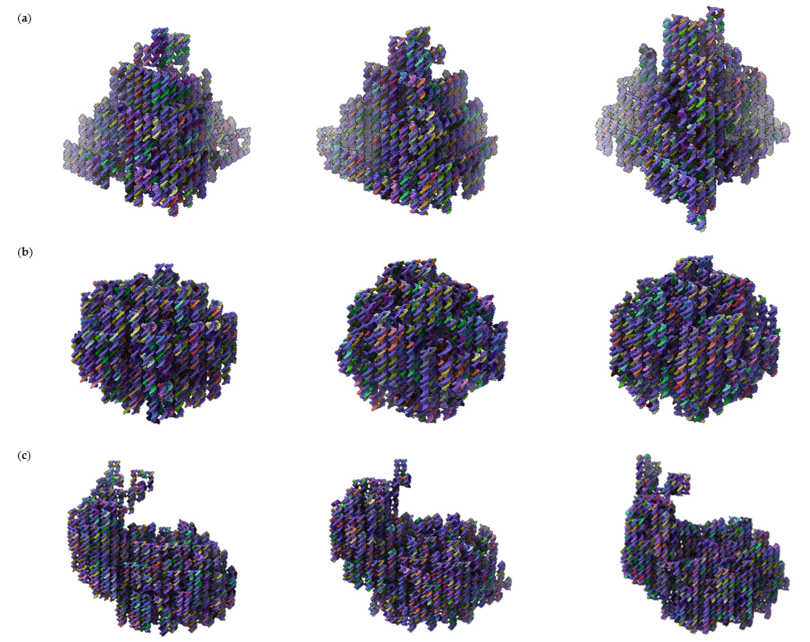
Figure 6.
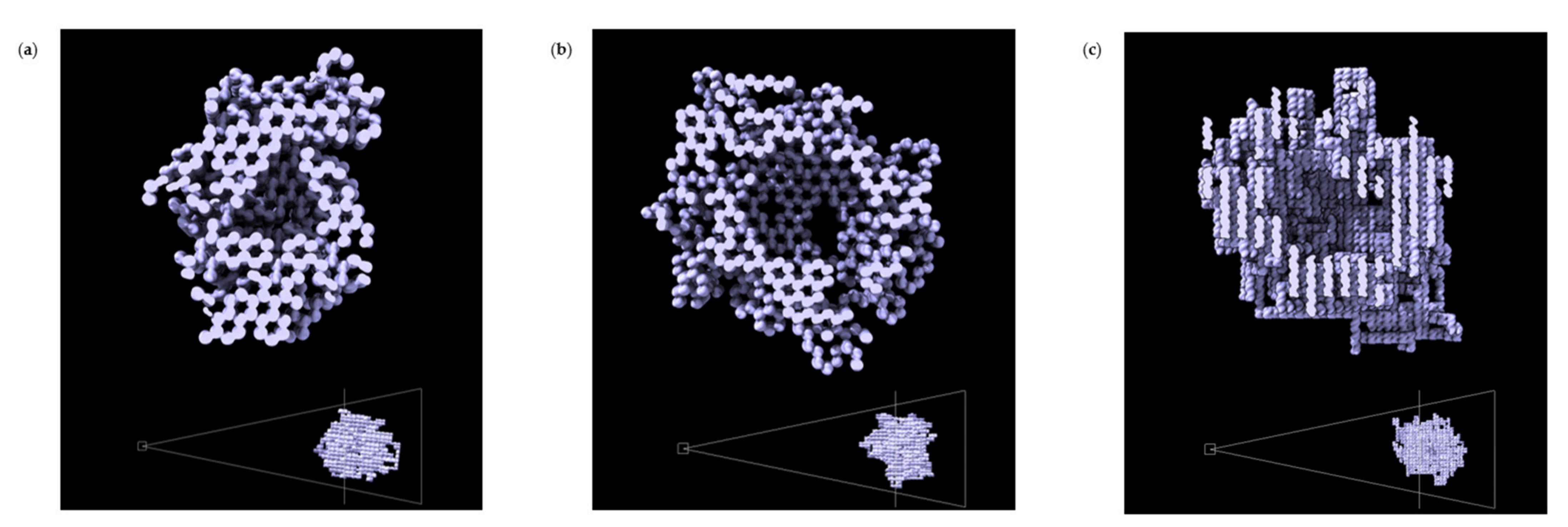
Isometric view of three of the best shapes generated per mesh with shape annealing algorithm for the filling application: (a) Structures generated with the tetrahedron mesh as the outer bounds of the design space. Each structure, from left to right, has a total length of 7595 bp, 7784 bp, and 7728 bp; (b) Structures generated with the snub cube mesh as the outer bounds of the design space. Each structure, from left to right, has a total length of 9275 bp, 8484 bp, and 8582 bp; (c) Structures generated with the Stanford bunny mesh as the outer bounds of the design space. Each structure, from left to right, has a total length of 14,595 bp, 13,531 bp, and 14,105 bp.
Figure 6.
Isometric view of three of the best shapes generated per mesh with shape annealing algorithm for the filling application: (a) Structures generated with the tetrahedron mesh as the outer bounds of the design space. Each structure, from left to right, has a total length of 7595 bp, 7784 bp, and 7728 bp; (b) Structures generated with the snub cube mesh as the outer bounds of the design space. Each structure, from left to right, has a total length of 9275 bp, 8484 bp, and 8582 bp; (c) Structures generated with the Stanford bunny mesh as the outer bounds of the design space. Each structure, from left to right, has a total length of 14,595 bp, 13,531 bp, and 14,105 bp.

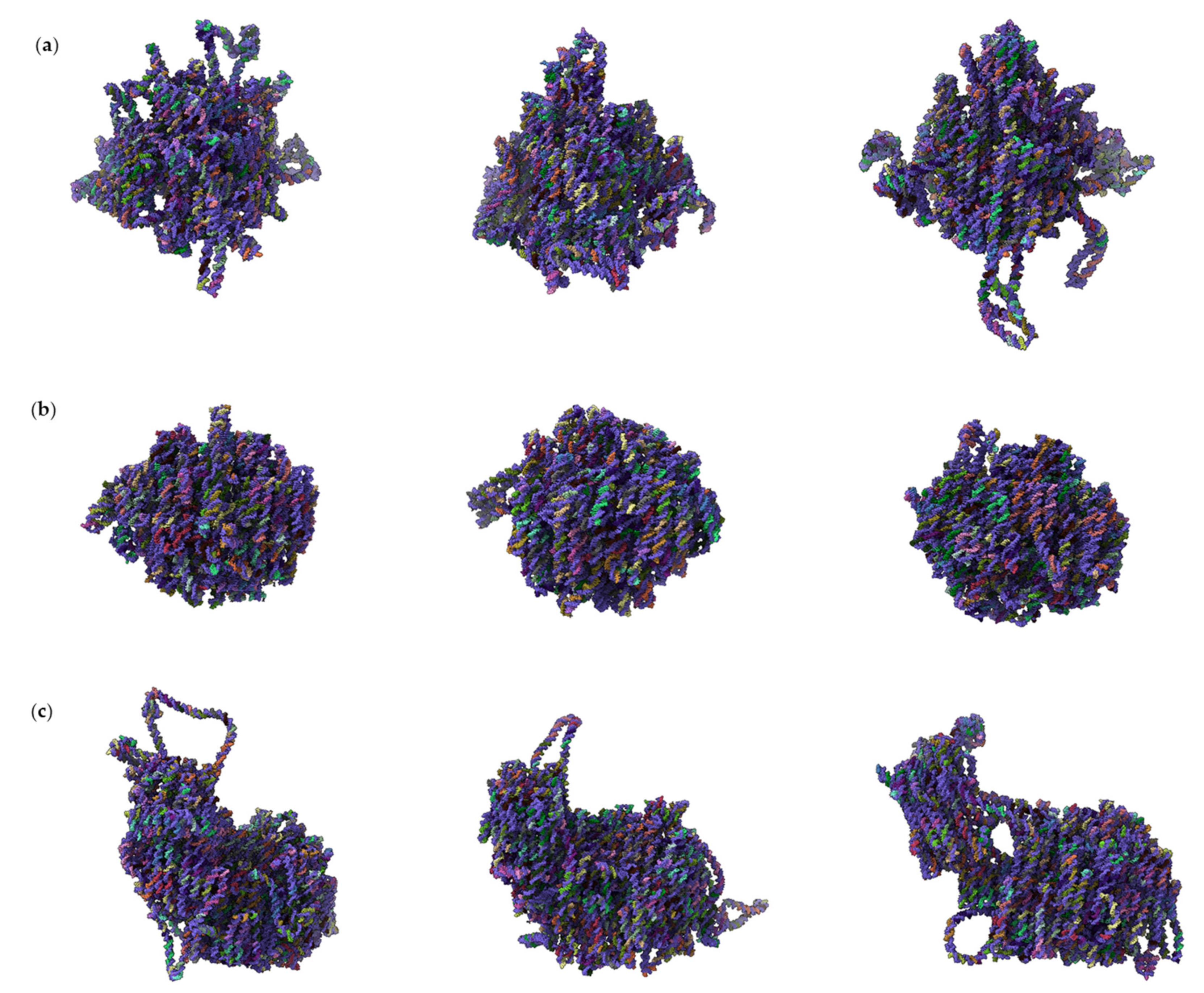
Figure 7.
Isometric view of fully relaxed configuration for filling application from oxDNA simulations (from Figure 6): (a) OxDNA 3D structure with the tetrahedron as the outer bounds of the design space. Each configuration, from left to right, has a total length of 7595 bp, 7784 bp, and 7728 bp; (b) OxDNA 3D structure with the snub cube mesh as the outer bounds of the design space. Each structure, from left to right, has a total length of 9275 bp, 8484 bp, and 8582 bp; (c) OxDNA 3D structure with the Stanford bunny mesh as the outer bounds of the design space. Each configuration, from left to right, has a total length of 14,595 bp, 13,531 bp, and 14,105 bp.

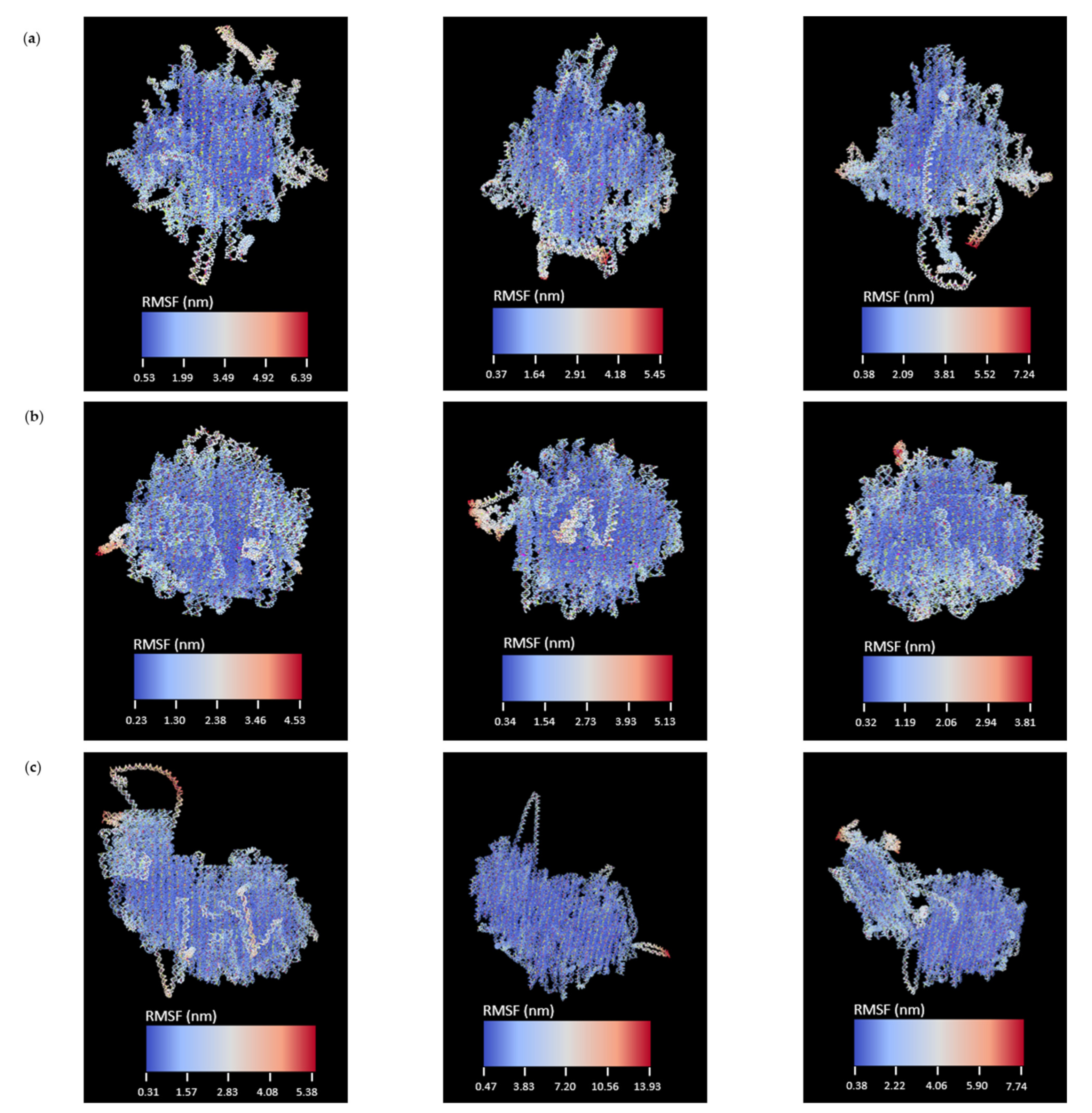
Figure 8.
RMSF of structures generated with filling application from Figure 6. The RMSFs are calculated relative to the average configurations generated over the entire trajectory. The images illustrate the patterns appearing in the RMSF calculations using a colormap with a smooth transition from a cool to warm color: (a) RMSF pattern for tetrahedron as the outer bounds of the design space. Each configuration, from left to right, has a total length of 7595 bp, 7784 bp, and 7728 bp; (b) RMSF pattern for snub cube mesh as the outer bounds of the design space. Each structure, from left to right, has a total length of 9275 bp, 8484 bp, and 8582 bp; (c) RMSF pattern for Stanford bunny mesh as the outer bounds of the design space. Each configuration, from left to right, has a total length of 14,595 bp, 13,531 bp, and 14,105 bp.

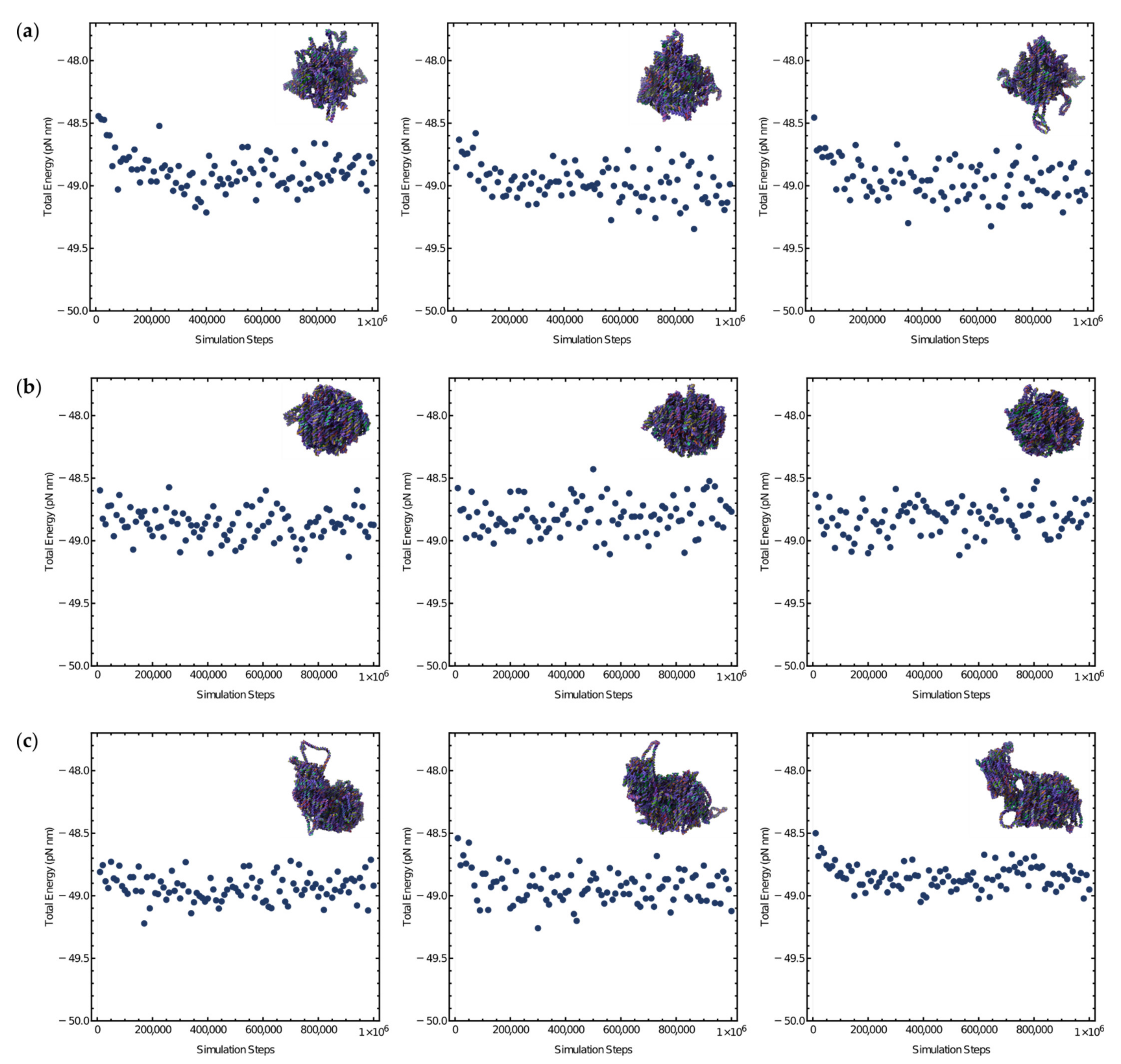
Figure 9.
Total system energy measurements (converted to pN nm from simulation units) over the course of the oxDNA relaxation step, corresponding to the structures in Figure 7 and Figure 8: (a) Plots for structures with the tetrahedron mesh as the outer bounds of the design space; (b) Plots for structures with the snub cube mesh as the outer bounds of the design space; (c) Plots for structures with the Stanford bunny mesh as the outer bounds of the design space. The plateauing of the total energy of the systems as it progresses through the relaxation simulation is an indication that equilibrium has been achieved. More anisotropic shapes with narrow features took longer to reach equilibrium.

Figure 10.
Isometric view of the best shapes generated with shape annealing algorithm for the coating application: (a) Slice view of structures generated with the tetrahedron mesh as the inner bounds of the design space with a total length of 12,901 bp; (b) Slice view of structures generated with the snub cube mesh as the inner bounds of the design space with a total length of 15,729 bp; (c) Slice view of structures generated with the Stanford bunny mesh as the inner bounds of the design space with a total length of 19,285 bp.

Figure 11.
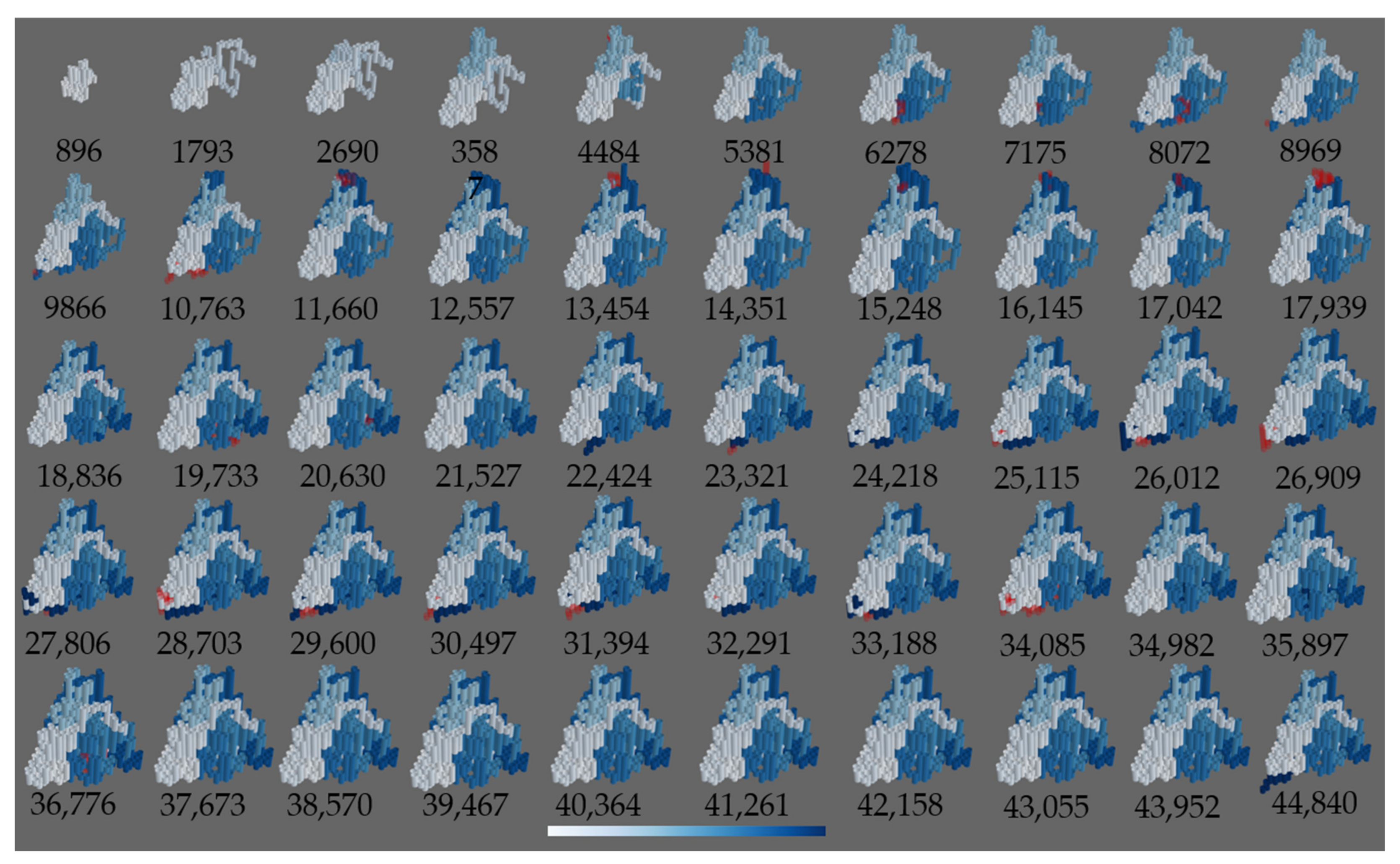
Scaffold growth visualization using a blue color map for right tetrahedron in Figure 6a with a total length of 7728 bp, where the scaffold is represented as cylinders. The total iteration of the shape annealing schedule is divided equally into 50 steps, where an image is generated at each step. The blue color map starts from a light blue tint, which represents the beginning of the scaffold, to dark blue tint, which represents the end of the scaffold. Below each image is the iteration number during the annealing schedule. The transparent red cylinders signify the application of the reversal rule.
Figure 11.
Scaffold growth visualization using a blue color map for right tetrahedron in Figure 6a with a total length of 7728 bp, where the scaffold is represented as cylinders. The total iteration of the shape annealing schedule is divided equally into 50 steps, where an image is generated at each step. The blue color map starts from a light blue tint, which represents the beginning of the scaffold, to dark blue tint, which represents the end of the scaffold. Below each image is the iteration number during the annealing schedule. The transparent red cylinders signify the application of the reversal rule.

Figure 12.
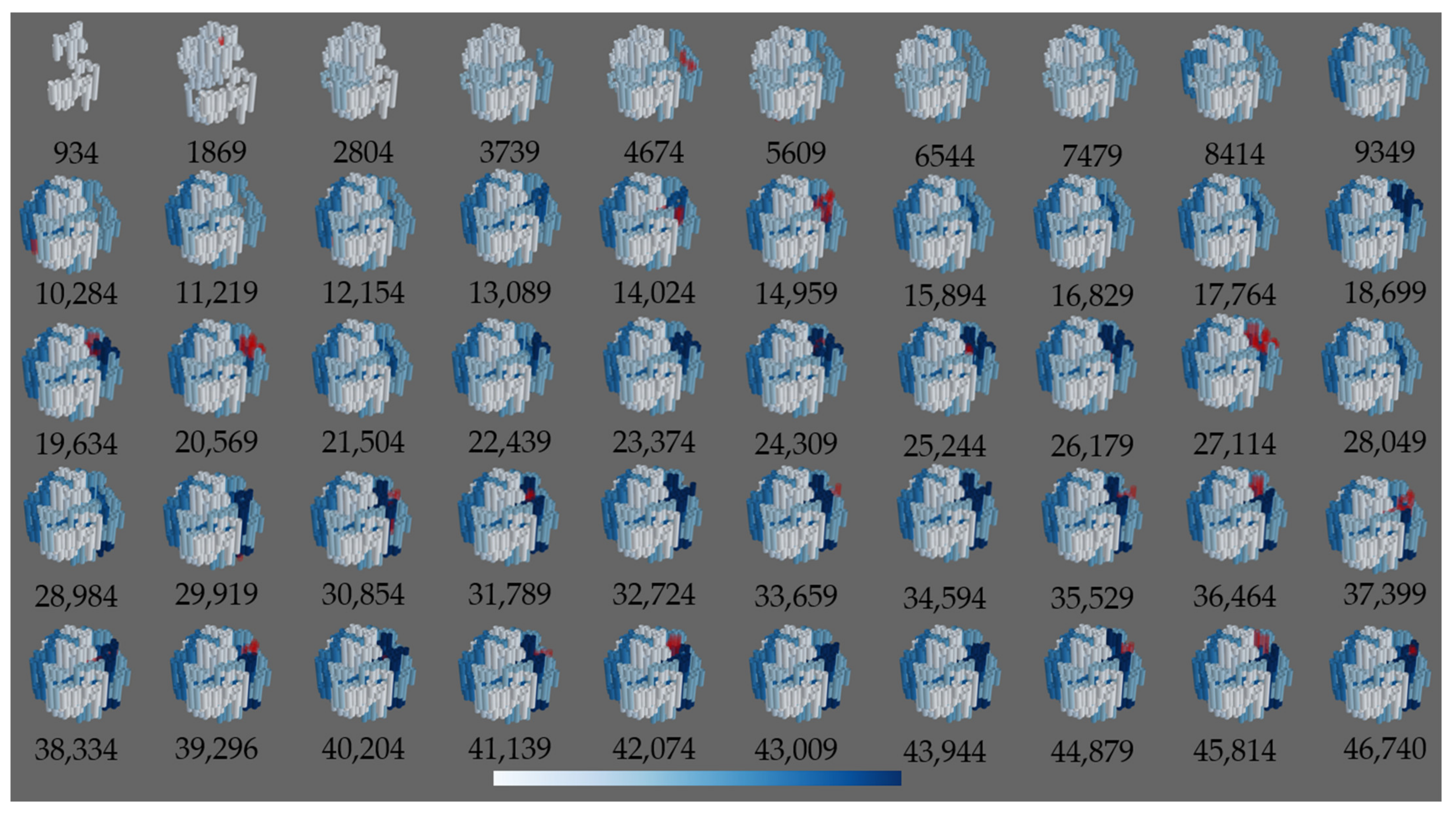
Scaffold growth visualization using blue color map for middle snub cube in Figure 6b with a total length of 8484 bp, where the scaffold is represented as cylinders. The total iteration of the shape annealing schedule is divided equally into 50 steps, where an image is generated at each step. The blue color map starts from a light blue tint, which represents the beginning of the scaffold, to dark blue tint, which represents the end of the scaffold. Below each image is the iteration number during the annealing schedule. The transparent red cylinders signify the application of the reversal rule.
Figure 12.
Scaffold growth visualization using blue color map for middle snub cube in Figure 6b with a total length of 8484 bp, where the scaffold is represented as cylinders. The total iteration of the shape annealing schedule is divided equally into 50 steps, where an image is generated at each step. The blue color map starts from a light blue tint, which represents the beginning of the scaffold, to dark blue tint, which represents the end of the scaffold. Below each image is the iteration number during the annealing schedule. The transparent red cylinders signify the application of the reversal rule.

Figure 13.
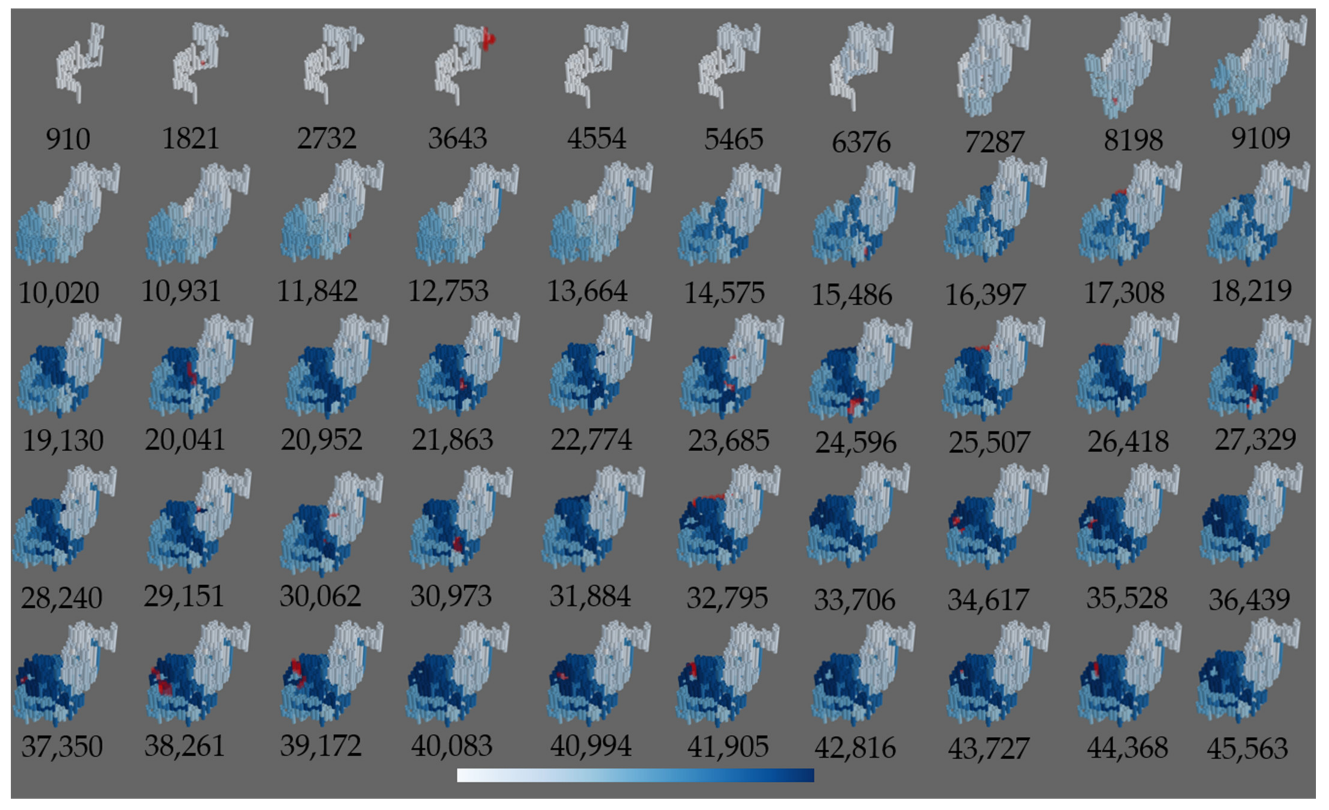
Scaffold growth visualization using blue color map for right Stanford bunny in Figure 6c with a total length of 14,405 bp, where the scaffold is represented as cylinders. The total iteration of the shape annealing schedule is divided equally into 50 steps, where an image is generated at each step. The blue color map starts from a light blue tint, which represents the beginning of the scaffold, to dark blue tint, which represents the end of the scaffold. Below each image is the iteration number during the annealing schedule. The transparent red cylinders signify the application of the reversal rule.
Figure 13.
Scaffold growth visualization using blue color map for right Stanford bunny in Figure 6c with a total length of 14,405 bp, where the scaffold is represented as cylinders. The total iteration of the shape annealing schedule is divided equally into 50 steps, where an image is generated at each step. The blue color map starts from a light blue tint, which represents the beginning of the scaffold, to dark blue tint, which represents the end of the scaffold. Below each image is the iteration number during the annealing schedule. The transparent red cylinders signify the application of the reversal rule.


Table 1.
Dimensions of input triangular mesh for coating application.
| Mesh | Length [nm] | Width [nm] | Height [nm] | |
|---|---|---|---|---|
| tetrahedron | 21.7 | 25.0 | 20.4 | 1840 |
| snub cube | 20.6 | 21.2 | 21.1 | 4010 |
| Stanford bunny | 32.4 | 26.0 | 32.2 | 7380 |
Table 2.
Average and standard deviation of total number of helical segments for filling application.
Table 2.
Average and standard deviation of total number of helical segments for filling application.
| Mesh | Average [Segments] | Std. Dev. | |
|---|---|---|---|
| tetrahedron | total | 875 | 159 |
| top | 1073 | 35 | |
| snub cube | total | 1076 | 135 |
| top | 1242 | 36 | |
| Stanford bunny | total | 1540 | 408 |
| top | 1981 | 84 |
Table 3.
Average and standard deviation of total number of helical segments close to mesh for coating application.
Table 3.
Average and standard deviation of total number of helical segments close to mesh for coating application.
| Mesh | Average [Segments] | Std. Dev. | |
|---|---|---|---|
| tetrahedron | total | 340 | 160 |
| top | 5 | 48 | |
| snub cube | total | 858 | 256 |
| top | 1134 | 54 | |
| Stanford bunny | total | 819 | 222 |
| top | 1086 | 81 |
Table 4.
Shape annealing optimization parameters.
| Application | Temperature (T) | Limit | α | Mutations (n) |
|---|---|---|---|---|
| filling | 80.00 | 35 | 0.99 | 310 |
| coating | 90.00 | 35 | 0.98 | 310 |
Publisher’s Note: MDPI stays neutral with regard to jurisdictional claims in published maps and institutional affiliations. |
© 2021 by the authors. Licensee MDPI, Basel, Switzerland. This article is an open access article distributed under the terms and conditions of the Creative Commons Attribution (CC BY) license (http://creativecommons.org/licenses/by/4.0/).
Share and Cite
MDPI and ACS Style
Babatunde, B.; Arias, D.S.; Cagan, J.; Taylor, R.E. Generating DNA Origami Nanostructures through Shape Annealing. Appl. Sci. 2021, 11, 2950. https://0-doi-org.brum.beds.ac.uk/10.3390/app11072950
AMA Style
Babatunde B, Arias DS, Cagan J, Taylor RE. Generating DNA Origami Nanostructures through Shape Annealing. Applied Sciences. 2021; 11(7):2950. https://0-doi-org.brum.beds.ac.uk/10.3390/app11072950
Chicago/Turabian StyleBabatunde, Bolutito, D. Sebastian Arias, Jonathan Cagan, and Rebecca E. Taylor. 2021. "Generating DNA Origami Nanostructures through Shape Annealing" Applied Sciences 11, no. 7: 2950. https://0-doi-org.brum.beds.ac.uk/10.3390/app11072950
Note that from the first issue of 2016, this journal uses article numbers instead of page numbers. See further details here.