All articles published by MDPI are made immediately available worldwide under an open access license. No special
permission is required to reuse all or part of the article published by MDPI, including figures and tables. For
articles published under an open access Creative Common CC BY license, any part of the article may be reused without
permission provided that the original article is clearly cited. For more information, please refer to
https://0-www-mdpi-com.brum.beds.ac.uk/openaccess.
Feature papers represent the most advanced research with significant potential for high impact in the field. A Feature
Paper should be a substantial original Article that involves several techniques or approaches, provides an outlook for
future research directions and describes possible research applications.
Feature papers are submitted upon individual invitation or recommendation by the scientific editors and must receive
positive feedback from the reviewers.
Editor’s Choice articles are based on recommendations by the scientific editors of MDPI journals from around the world.
Editors select a small number of articles recently published in the journal that they believe will be particularly
interesting to readers, or important in the respective research area. The aim is to provide a snapshot of some of the
most exciting work published in the various research areas of the journal.
Current trends in electrification of the final energy consumption and towards a massive electricity production from renewables are leading a revolution in the electric distribution system. Indeed, the traditional “fit & forget” planning approach used by Distributors would entail a huge amount of network investment. Therefore, for making these trends economically sustainable, the concept of Smart Distribution Network has been proposed, based on active management of the system and the exploitation of flexibility services provided by Distributed Energy Resources. However, the uncertainties associated to this innovation are holding its acceptance by utilities. For increasing their confidence, new risk-based planning tools are necessary, able to estimate the residual risk connected with each choice and identify solutions that can gradually lead to a full Smart Distribution Network implementation. Battery energy storage systems, owned and operated by Distributors, represent one of these solutions, since they can support the use of local flexibility services by covering part of the associated uncertainties. The paper presents a robust approach for the optimal exploitation of these flexibility services with a simultaneous optimal allocation of storage devices. For each solution, the residual risk is estimated, making this tool ready for its integration within a risk-based planning procedure.
With the ambition of achieving a net-zero greenhouse gas emissions by 2050, European Union planned several actions aimed at realizing high shares of renewable energy use (28% by 2030 and 66% by 2050) and of heat and transport electrification (exceeding 50% by 2050) [1,2]. Despite the COVID-19 pandemic has caused a fall in electricity consumption [3], the power generation from renewable energy sources (RES) continues its accelerating expansion [4], keeping valid the general goal of increasing loading and hosting capacity of the electric distribution systems. Indeed, a massive production from RES, often non-homothetic with electric demand, and the expected peak load increment due to the electrification of end uses will impact the distribution system operation by worsening voltage profiles and stressing cables and transformers. It is worth noting that this scenario will strongly affect also the bulk power system that needs stable generation support, increasing reserves and ramping services for compensating the decommissioning of polluting conventional generation, consequence of the RES development [5].
Flexibility is the backbone of the electricity system and the current transition of its availability from conventional large power plants to Distributed Energy Resources (DERs) will introduce new challenges to be faced [6]. Undeniably, DERs could support grid operation, selling their flexibility through the participation in wholesale markets [7], but by so doing they may cause technical issues into the distribution system. Therefore, suitable coordination procedures should be implemented between Transmission and Distribution System Operators (TSO and DSO), always considering the option for the DSO to exploit part of the flexibility from DERs for the secure operation of their local networks. Indeed, the alternative of an oversized distribution system that enables TSO the unilateral and unrestricted use of this flexibility could be economically unsustainable.
In addition, recent EU directives 2019/944 (art. 32) [8] has stated that “network development plan shall also include the use of demand response, energy efficiency, energy storage facilities or other resources that distribution system operator is to use as an alternative to system expansion”, legitimating the exploitation of flexibility services from DERs as a planning solution for the future Smart Distribution Network (SDN), as anticipated by the scientific community [9,10,11].
Flexibility can be defined as the capability of a coordinated multitude of actors to change their behaviour for providing support to the bulk power system operation or to the distribution system management. It comes from the users of the distribution network (loads, generators, stationary storage devices), from sector coupling (electric vehicles, electric boilers, heat pumps and electrolysers for hydrogen production) or from the network itself (network reconfiguration, online tap changer of secondary substations, line voltage regulators). More specifically for the flexibility from DERs, flexible loads may shift in time or curtail (increase) their electricity consumption when participating to Demand Response (DR) programs, flexible generators can curtail (photovoltaic or wind) or shift in time (CHP) their electricity production, and flexible storage may behave like a flexible load or a flexible generator depending on system needs.
As aforementioned, modern DSO needs to consider these flexibility services from local DERs for solving possible contingencies and it needs also to quantify how much they cost, compared to conventional planning actions based on network reinforcement. However, this comparison must be based also on the risk of these new planning choices, because one common question from all distribution system actors is how much reliable the flexibility from DER will be. Indeed, many uncertainties characterize this future scenario like the actual response of many private resources (consumers and producers) to service requests from the DSO, the organization of the local ancillary services market (if any), and the prices of the new services. Therefore, it is plausible that DSOs wish to start this revolution gradually by introducing solutions that can help limiting the risk associated to this flexibility. Even if not yet exploited, one option available in the current European regulation can be the installation of storage devices directly operated by the DSO. It represents a particular network investment which can be used for many applications simultaneously (losses reduction, peak shaving, voltage regulation) and, in this case, it can increase the flexibility of the secondary substation where it is installed, reducing at the same time the uncertainty of this flexibility exploitation.
Following these considerations, ad hoc risk-based tools must be developed for the optimal expansion planning of distribution systems, able to assess the overall technical constraints violation risk of a given network and the residual risks associated to different planning solutions. The first kind of assessment has been formalized in [10] and a possible implementation, proposed by the authors in previous research [12,13,14], has been briefly described in Section 3. The second calculation, coupled to the optimal exploitation of flexibility services from DERs, is deeply illustrated in Section 4 and constitutes the main novelty of the paper. This procedure is based on a Robust Linear Programming (RLP) for modelling the uncertainties related to the active management of DER and estimating the residual risk associated to each optimal solution identified. Two type of uncertainties have been considered: the forecast errors of some data entry (the prices for remunerating the flexibility services) and the actual DERs response to a flexibility request from the DSO.
Robust Optimization (RO) is a complementary methodology to traditional Sensitivity Analysis and Stochastic Optimization to deal with uncertainties that affect the data of real-world optimization problems. The success of this approach comes from the not required distribution assumptions on uncertain parameters and the computational tractability of the robust formulation of Linear Programming problems [15]. For these reasons, in the last decade RO has been applied to several optimization fields, including power systems. Regarding DERs, RO has been often used to model the uncertain behaviour of load consumption and RES production within specific problems: the optimal energy storage system location [16], the optimal demand bidding under uncertain market and including distribution network operational limits [17], the generation and transmission expansion planning problem [18]. When dealing with the flexibility provided by DERs, RO has been applied from the aggregator point of view for maximizing the flexibility potential of its customers to provide services to other actors [19] and to minimize day-ahead operation costs while complying with energy commitments in the day-ahead market and local flexibility requests [20]. To the best of authors’ knowledge, RO has not been yet applied from the DSO point of view to model the uncertain provision of flexibility services used for distribution network planning.
In summary, the present work proposes a RLP for the minimization of the procurement costs of flexibility services from DERs used to solve possible technical issues in the distribution network. The tool is ready for the integration in a wider risk-based planning tool for SDN. Particular attention has been paid to the assessment of the residual risk of the optimal solution, due to the uncertain provision of flexibility services. The objective function of the RLP implements an economic model of the flexibility services remuneration, based on capacity and energy terms. To reduce the uncertainty of the flexibility services provision, the DSO has also the possibility to install and operate some Battery Energy Storage Systems (BESSs). For this reason, the objective function of the RLP has been built to also find the optimal rate and location of these devices, identifying an economic balance between flexibility services exploitation and BESS investment.
The paper is organised as follows. Section 2 describes the theoretical bases of the RO and of its probabilistic guarantees. Section 3 briefly illustrates the risk-based planning tool, while Section 4 details the implementation of the RLP for the flexibility services exploitation. In Section 5 some case studies derived from real Italian distribution network and adopted for testing the proposed approach have been specified. Section 6 analyses and discusses the results obtained and, finally, Section 7 provides some concluding remarks and topics for the future research.
2. Robust Optimization
For typical real-world problems where system operation and components’ responses may deviate from the ideal ones, decision-maker wishes to identify optimal solutions that protect himself against parameter variability and implementation uncertainty. This issue becomes of paramount importance when new technologies and innovative problem solutions are introduced, due to the lack of information on the on-field performances of the new devices or on the actual behaviour of the actors involved. Different mathematical approaches have been proposed in literature and applied into practice, such as Sensitivity Analysis, Stochastic Programming, Chance-Constrained methods, and Robust Optimization.
The burgeoning success of RO in a wide selection of application areas lies in its computational tractability because the uncertainty model adopted is not stochastic, but rather deterministic and set-based. Instead of striving for a probabilistic immunization of the solution to stochastic uncertainty, it creates a solution that is feasible for any realization of the uncertainty in a given set. From this point of view, RO is a worst-case oriented methodology, and this aspect also determines its main drawback: the possible over-conservatism of the solution. Thus, the choice of the uncertain parameter set into which the worst-case is evaluated should be done to achieve an acceptable trade-off between system performance and protection against uncertainty, i.e., neither too small nor too large.
For a Linear Programming (LP) optimization, the robust counterpart is written as:
where x is the vector of decision variables, A is a m × n constraint matrix, is the right-hand-side vector, η is a random variable, Ξ is the entire uncertain set and U is the uncertainty subset of Ξ used for the optimisation. The desired protection level against uncertainty depends on the extent of Ξ covered by U. For instance, if the goal is the maximum protection (no risk of constraints violation, i.e., worst-case scenario), then the robust optimisation has to consider simultaneously all possible variations of the input data and, accordingly, U ≡ Ξ. However, this option is generally over-conservative, because it also considers combinations of parameters’ values that are extremely rare to happen. Therefore, if a minimum risk is acceptable, a subset of Ξ can be used.
In formulation (1), data uncertainty is supposed to affect only the elements of matrix A, because the possible uncertainty in the objective function (c vector) can be easily moved among the inequality constraints by changing the objective function () and adding a new constraint ().
The generic uncertain coefficient ãij of matrix A is modelled as a symmetric and bounded random variable that varies in the interval [aij − âij, aij + âij], where aij is the nominal value of ãij and âij is the extreme deviation from the nominal value. The hypothesis of modelling uncertainty with symmetric and bounded random variables is necessary to preserve the convexity of U [21]. Associated to the uncertain coefficient ãij, it is defined the random variable ηij = (ãij − aij)/âij, which follows an unknown, but symmetric, distribution and takes values in [–1, 1].
By indicating with Ji the set of uncertain coefficients (ãij) in the ith row of the matrix A, the generic inequality constraint of the LP problem (1) can be written as:
where l and u are the lower and upper bound vectors of the variables x. The introduction of the variable yj is motivated when xj can assume negative values (lj < 0), as explained below. The second addendum of the inequality constraint in Equation (2):
represents the worst-case term. In other words, it can be said that the ith constraint is protected by βi(x,U) against the uncertainty of the parameters ãij. Hence, the robust counterpart is a bi-level problem, and its tractability is affected by the geometry of the uncertainty set U because the way in which the inner maximization in Equation (2) is eliminated depends on it. Several choices are available in literature: box, ellipsoidal and polyhedral sets (Figure 1).
The box set corresponds to the maximum possible protection level and assumes that all parameters will take the worst possible value (worst case scenario). It is the most straightforward approach but also the most conservative, with the highest deterioration of the objective function (Figure 1a). To address the excessive conservatism of the box set, an ellipsoidal uncertainty set has been proposed on the observation that corners tend to be unlikely to happen (Figure 1b). However, due to the non-linearity of the model, it leads to computationally complex robust counterparts (Second Order Conic Problem). The polyhedral representation constitutes a compromise between the two previous models because it still allows controlling conservatism while preserving computational tractability [22]. The idea behind this model is that, even if every uncertain parameter can always assume the worst-case value, only a few of them does it simultaneously, and their number is controlled by the so-called Uncertainty Budget, Γ (Figure 1c).
Because in practice uncertainties are generally bounded, and it is useless to consider parameters’ values that exceed the uncertain space Ξ, it is generally convenient defining uncertainty sets generated by combining the ellipsoidal or polyhedral set with the box set. In the paper, for limiting the computational burden, the “box + polyhedral” model has been adopted (Figure 1d). For Γ = 1, the polyhedron is exactly inscribed by the box, and the intersection between the two sets is exactly the polyhedron; on the contrary, when Γ = |Ji|, the box is exactly inscribed in the polyhedron, and the intersection between them is exactly the box. With this kind of model, it is possible to show that the ith constraint of the robust counterpart, Equation (2), is equivalent to the following formulation:
where the auxiliary variables zi and wij are used to eliminate the inner maximization by using its dual formulation. This process requires resorting to the absolute value |xj|. If the variable is positive, the absolute value operator can be directly removed. Otherwise, it can be eliminated by introducing an additional auxiliary variable yj and the constraint −yj ≤ xj ≤ yj:
Probabilistic Guarantees in Robust Optimization
Differently to the stochastic optimization, RO does not provide explicit control on the risk of constraint violation. Therefore, it is crucial to define a probabilistic guarantee for the robust solution that can be computed a priori as a function of the structure and size of the uncertainty set. Indeed, the quality of an optimal solution relies on the definition of uncertainty sets that are guaranteed to satisfy a particular upper bound on the probability of constrain violation: a tighter probabilistic bound allows the adoption of a smaller uncertainty set with the same guarantee of feasibility and, consequently, leads to a less conservative solution.
Some theoretical a priori upper bounds () for the probability of constraint violation have been proposed in literature. One of the most common is given by:
where Δi is the adjustable parameter of the specific uncertainty set adopted (e.g., Γi for the box + polyhedral set), and |Ji| is the total number of uncertain parameters in the ith constraint [23]. While this bound is appealing for its simplicity, it is not so attractive for its over-conservatism, especially when the number of uncertain parameters in a given constraint and the acceptable risk are small. For instance, with the box + polyhedral uncertainty set, 6 uncertain parameters and an accepted violation constraint probability of 10%, the uncertainty budget Γi calculated from (6) is around 5.3 (Figure 2), almost equivalent to the box set representation, where all uncertain parameters are assumed at their worst extreme value (worst-case scenario).
The sole assumption used to derive the bound (6) is that the uncertain parameters are bounded and have known means. If the postulation of symmetric distribution is added, a better upper bound for a box + polyhedral uncertainty set has been derived in [24] and it is expressed as:
where
As it can be seen from Figure 2, bound (7) is clearly tighter, so providing “less conservative” solutions. For the previous example, the uncertainty budget Γi is taken equal to 4.001, i.e., 4 of 6 uncertain parameters are allowed to assume their worst value and one can change by 0.001 of its extreme deviation to guarantee a risk of constraint violation that does not exceed 10% probability.
A second approach for assessing the probabilistic guarantees is based on the solution of the RO problem (x*), and for this reason the resulting bound is called a posteriori bound (). It is typically used for checking the probability of constraint violation of the results obtained with specific uncertainty sets defined by a priori probabilistic bounds. Indeed, a posteriori bound will provide probabilities that are as tight as or tighter than those provided by the a priori bound, but only when they are “analogous”, i.e., the two bounds have to be derived with the same procedure and based on the same assumptions. For the a priori bound expressed in Equation (7), two ways exist to extend its principles to a posteriori bound. The analogue a posteriori bound of (7) is:
where
In Equation (8), is a parameter used for the proof of the upper bounds and its definition depends on the uncertainty set adopted: the definition reported in Equation (8) is related to a polyhedral + box set and makes . The subscript r corresponds to the index of the largest . Essentially, it is scaled by a factor related to the specific uncertainty set. The vector represents the solution of the robust optimization.
However, in [24] it is observed that Equation (8) does not provide the expected reduction in the a posteriori risk when (that is the case of polyhedral and polyhedral + box sets) or when the ith constraint is inactive. An alternative formulation of the a posteriori bound is:
where
But, even if it generally provides lower probabilities than Equations (8) and (7), it is not exactly the analogue of Equation (7), and thus it can yield higher a posteriori probabilities. Therefore, it is always preferred to apply both the Equations (8) and (9) and take the minimum probability generated.
3. Risk Assessment of Technical Constraints Violation
An explicit and detailed assessment of the annual risk to violate technical constraints in a given distribution network requires a stochastic network analysis, which makes use of ad-hoc probabilistic descriptions of customers’ uncertain behaviour. Firstly, their yearly variability has been represented through typical days (with discretization of one hour) that capture the daily, weekly, and seasonal changes in electricity consumption or production, so reproducing the positive and/or negative interactions among loads and non-dispatchable renewable energy sources and the operational impact of the flexibility services. Secondly, their hourly uncertainty has been modelled by assuming Gaussian probability distribution. Consequently, Probabilistic Load Flow (PLF) calculations have been solved for each time step of typical days [12], to identify any critical operating condition with its occurrence probability and to correctly assess the results of possible remedy actions.
The risk assessment procedure (flow chart of Figure 3) starts with the definition of the impedance matrix [Z]b, relative to the bth network configuration in the N − 1 security analysis (where b = 0 means the network in normal configuration and b > 0 means the network reconfigured without the bth element), and the acquisition of the nodal current matrix [Inode]f in the fth hour of the typical daily profile. The results of the PLF are the nodal voltage [Vnode]f and the branch current [Ibranch]f matrixes (expressed in terms of mean value, μ, and standard deviation, σ, of a normal distribution), by which the probability (ptcv) to overcome the voltage regulation band [Vmin, Vmax] or the conductor ampacity (Imax) is estimated. Only the Nc operating conditions with non-negligible probability to violate the technical constraints (ptcv > 0) are stored (Figure 3—case A), while the cases on which the extremes values of any nodal voltage and branch current (, and ), assumed equal to μ ± 3σ, do not exceed the technical limits are disregarded (Figure 3—case B).
In order to calculate the risk of technical constraints violation (Rbf) when the bth network configuration is in force during the fth hour, the ptcv is multiplied by the occurrence probability (pbf) of the relative operating conditions. The sum of all these risk components, determined for each configuration in each interval of the typical days, forms the total risk (RT) that characterises the distribution network examined, i.e., the number of hours per year when it is possible to overcome a technical constraint. When the total risk is greater than the acceptable limit fixed by the DSO planner, RA, planning solutions must be put in place to reduce RT below RA and make the distribution network robust enough for the whole planning period considered.
Each potential contingency is faced by resorting separately to both flexibility services from DERs and network reinforcement (upgrade of existing conductors or transformers), with the goal of minimizing residual risk. The paper is focussed on the first kind of solutions, by developing an optimization tool able to find the correct amount of flexibility, taking account of the uncertainties that may characterize the behaviour of the resources involved.
4. Robust Exploitation of Flexibility from DER and Its Residual Risk
The focus of the paper is on the new category of remedy actions: the active management of the available energy resources in a given distribution system. Specifically, generation curtailment and demand response are the flexibility services that DSO can purchase from a local ancillary services market to solve network contingencies. In previous works, the problem of the optimal flexibility exploitation has been solved with a Linear Programming (LP) approach that minimizes a cost-function, CFlex, expressed as the weighted sum of the flexibility services subject to network constraints:
In model (10), α and β are weights proportional to the cost of the corresponding flexibility service, is the curtailed electricity production from the gth Renewable Energy Source (RES), is the curtailed electricity consumption from the dth customer involved on the DR programme, and are the maximum flexibility offered by the gth RES and the dth customer, NRES and NDR are respectively the number of RES and of customers available to provide flexibility services, NN and NL are respectively the total number of nodes and lines in the distribution network, and are the sensitivity coefficients of the voltage in the ith node and the current in the jth branch with respect to the active power variation of a generic DER, and is a function that associates the ordinal number of a DER with the cardinal number of the network node where it is connected.
To be more precise about the sensitivity coefficients, each of them has been assessed by comparing the PLF results in the initial conditions with those of a second PLF obtained by reducing the active power consumed in a single node. With this procedure, the voltage sensitivity coefficients are always negative and, by assuming positive the line currents that flow downstream from the primary substation and negative the line currents that flow in the opposite direction, the current sensitivity coefficients are always positive. Thanks to these observations and considering that all the active power variations in the LP problem (10) are positive (decision variables), the effect of a generation curtailment is inserted in the corresponding inequality constraint with the plus sign (i.e., if generation is reduced, the nodal voltage decreases), while the effect of a DR programme is included with the minus sign (i.e., a load reduction causes a voltage increase). The inequality constraints for the maximum line currents have been doubled to eliminate the absolute value that should be used for the left-hand-side of these inequalities (indeed, it is important the magnitude of the line current and not its direction). It must be noted that, due to the electric characteristics of distribution networks, the sensitivity coefficient is practically invariant with respect to the amount of active power variation used for the second PLF calculation. This aspect allows considering the sensitivity coefficient as constant parameters, so preserving the linearity of the inequality constraints in Equation (10).
Starting from this basic formulation, additional improvements have been included in the paper to enlarge the flexibility options, refine the models and take account of the flexibility exploitation uncertainties. First, the objective function has been expanded to include also the BESS that DSO can install in its system. Because it is an energy resource owned by the DSO, only its investment has been added to CFlex, while its operation has been considered in the inequality constraints. Secondly, a new market model has been assumed, where the flexibility remuneration is expressed both in capacity and in energy. In other terms, when a specific DER is enabled to participate to the local ancillary services market, it is initially remunerated for the capacity made available within a time-interval (e.g., a week, a month, a year), and then it is also remunerated each time it is called to provide the service. With these improvements, a first upgrade to the objective function can be formulated as:
where and are the prices for the capacity remuneration of the gth RES and the dth customer expressed in €/(kW·year), and are the prices for the energy remuneration of the gth RES and the dth customer expressed in €/(kWh), Rb,h is the risk of constraints violation expressed in hours per year in the bth network reconfiguration during the hth hour, T is the time-interval considered (e.g., the 24 h of a typical day, the repair time of a faulted element that causes a specific emergency network reconfiguration, or simply the single time-step that manifests a contingency), Δh is the time-step used to discretize T (typically 1 h), cp and ce are the power and energy unitary cost of BESS, and are the nominal power and the nominal capacity of the BESS installed in the kth node, and AF is the annuity factor used to convert a single investment into an annual expenditure and allow the comparison between the BESS investment and the annual cost for flexibility services procurement. By assuming a duration of the investment of n years, equivalent to the lifespan of the BESS, and a constant interest rate (r), AF is evaluated as:
The factor Rb,h is the risk component calculated with the flowchart of Figure 3 and it is used to estimate the annual recourse to flexibility services and, consequently, its energy remuneration. The extension of the optimization to multiple time-steps simultaneously (T > 1) is motivated by the potential presence of multiple contingency events during the same network operating conditions (b) and, consequently, the need to correctly assess the capacity remuneration and the BESS sizing. Indeed, the resort to a flexibility resource may have different energy requests for different time-steps within the same time-interval T but it must have the same capacity bid. Also, if two time-steps with Rb,h > 0 are close or one next to the other, the BESS must be sized for solving sequentially both the contingencies.
In summary, the new problem statement (11) will define the optimal compromise between the investment in BESS (finding number, site, and size of storage devices) and the purchase of flexibility services from existing DERs (in terms of capacity available and energy used). A further improvement of the economic model has been obtained by fixing a cap in the annual budget available for the DSO (Bcap). This cap can be fixed arbitrarily, or it can derive from the conventional planning alternative of network refurbishment. In other words, it can be used to compare the investments in network solutions, needed to solve the technical issues, with the expenditures in flexibility services (e.g., DR actions) and in innovative solutions (BESS). Obviously, also Bcap is assessed by applying a suitable annuity factor to each network upgrade.
This new constraint increases the possibility that the LP problem becomes unfeasible due to the lack of sufficient resources to solve all the contingencies. It is important to note that these defective situations have not to be disregarded but they are still useful in a general planning procedure. Indeed, even if the risk of constraints violation is not nullified, it is reduced (residual risk) so contributing to the achievement of the planning goal of RT < RA. To overcome this limitation and allow the optimization to provide always a solution, “slack” variables have been introduced in the objective function and in the nodal voltage and line current inequality constraints (). Dimensionally, they represent the residual gaps in nodal voltages or in line currents that the available DERs are not able to close for satisfying the corresponding technical constraints. In the objective function, they are weighted by a very large cost, to avoid that they could be used needlessly, i.e., when flexibility resources are still available below the budget cap. When returned (≠0) by the LP optimization, they allow assessing the residual risk through the probability density function of the corresponding nodal voltage or line current. For instance, referring to Figure 4, the existing probability to overcome the maximum nodal voltage () is reduced to the red striped area that corresponds to the occurrence probability of the operating conditions that bring the ith nodal voltage within the gap not solved by the available DERs ().
Taking account of all these improvements, the full deterministic formulation of the optimal exploitation of flexibility from private DERs and from BESS owned by the DSO is expressed by the following LP problem:
In the inequality constraints (15), the contribution of BESS operation is inserted with the plus sign, because, when , the storage is charging () and its effects is equivalent to a generation curtailment and, when , the storage is discharging () and its effects is equivalent to a load curtailment. The group (16) includes all the technical constraints of the resources (the active power of the BESS absorbed from or released to the grid must be lower or equal to the nominal power of the storage device, the state of charge must be always within an acceptable band of operation, the initial state of charge has to be equal to the last value when considering the whole typical day) and the external data fixed by the operator (the ranges of power, [, ], and duration, [, ], for the BESS sizing, the minimum and maximum states of charge defined as percentage of the BESS capacity, σm and σM, the BESS round-trip efficiency, ηtrip, and the maximum amount of flexibility that each resource makes available, and ). It has not been considered a minimum size for the BESS power, in order to optimize also the location and not only the size of the storage. Indeed, when , no BESS is in the kth node. If a minimum size needs to be fixed preserving on the same time the siting optimization, a Mixed Integer Linear Programming formulation should be implemented.
As aforementioned, this LP formulation is deterministic, in the sense that all data are exactly known, and the operation of each resource is certain. However, this is a weak assumption, and several uncertainties still affect this model, because the active management of DER is not yet implemented in the actual distribution system (only few pilot projects have been founded in the last years), and local ancillary services markets does not exist. Therefore, the estimation of the risk associated to the exploitation of flexibility from DER is becoming of paramount importance for overcoming the last concerns of the DSO and arranging feasible and economic implementation plans. Due to the lack of practical experience, it is extremely difficult defining stochastic models to represent the uncertain aspects and RO represents one of the few alternatives to face this optimization problem. Indeed, it is worth to remind that for RO it is not necessary to know exactly the uncertainty distribution, but it is sufficient the assumption of symmetric and bounded random variables. In the paper, two kind of uncertainties have been considered: a prediction uncertainty and an implementation uncertainty [15].
The first category generally depends on the forecast errors of some data entries that do not exist when the problem is solved. For the LP problem (13), these parameters are the prices used for assessing the remuneration of the flexibility services (, , and ) that will be represented as symmetric and bounded random variables, whose range of uncertainty is influenced by the market organization decided by the regulation authority.
The second type of data uncertainty occurs when some of the decision variables cannot be implemented exactly as computed. This is the case of the DER responses to the flexibility requests from DSO ( and ), which may differ from the ideal values calculated due to the partial unavailability of the flexibility offered. These errors can be represented as equivalent to appropriate artificial data uncertainties. Indeed, reminding that the contribution of a particular decision variable xj to the ith constraint is the term aijxj, a typical multiplicative implementation error can be rearranged as no implementation error on the decision variable and uncertainty applied to the data coefficient . For making the equations of the LP problem more legible, the uncertain parameters have been renamed as following:
where a is the expected value of the uncertain parameter ã and â is its extreme variation.
Observing that uncertain parameters also affect the objective function (13), this last has been changed and a new constrain has been added for leaving uncertain coefficients only among the elements of matrix A. Moreover, all constraints have been rearranged as “≤” inequalities to preserve the canonical formulation (). By so doing, the uncertain formulation of (13)–(15) is:
The group of constraints (16) remains valid and unaltered, so it has not been repeated just for simplicity. The uncertainty set size of constraint (19) is , while the number of uncertain parameters for the generic nth inequality of group (21) is .
Finally, the robust counterpart of the LP optimization used to find the robust exploitation of flexibility from DER has been obtained by applying model (4). To avoid a tedious and repetitive mathematical description, only the application to constraint (18) has been shown:
The uncertainty budget Γn has been calculated for each uncertain constraint based on a prefixed maximum acceptable risk (upper bound ) by using Equation (7). Finally, the a posteriori risk () is determined by taking the minimum value between Equations (8) and (9). When too few resources are available or the budget limitation Bcap is too tight, the total residual risk may become higher than the prefixed a priori value, because the calculated a posteriori risk will be incremented by the highest probability associated to the non-zero slack variables (red striped area of Figure 4).
5. Case Study
The methodology proposed has been applied to a case study derived from a real Italian Medium Voltage (MV) distribution network, adequately clustered to reduce the number of secondary substations from 80 to 21 (Figure 5). It is a rural distribution system, radially operated, with two feeders in normal operating conditions (F1 and F2), fed by a Primary Substation with a 16 MVA (132/20 kV) transformer, and interconnected by a tie-line normally open (branch 4–15).
Long overhead lines supply small loads. The conductor’ cross-sections (S) are relatively small due to the low load density, and voltage drop issues can be expected. Three PV generators are also connected that may cause overvoltages. Table 1, Table 2 and Table 3 summarize respectively the data of customers, branches and conductors. The trunk conductors in an open-loop topology are sized with a constant cross-section (typical practice of the main Italian DSO), so that all the secondary substations can be resupplied for the outage of any trunk branch. Four different kind of customers are connected to the system: the predominant category is the residential (11 secondary substations), followed by agricultural (6), tertiary (2) and industrial (2). Their typical load profiles have been taken from the daily curves of the ATLANTIDE project [25], as depicted in Figure 6.
Only one typical day has been used to simulate the customers’ behaviour along the whole year. Their hourly variability has been represented by a Gaussian distribution with a mean value reported in the figure and a constant standard deviation of 5%. Obviously, more detailed representations are possible (multiple typical days for catching the weekly and seasonal variability, different standard deviations along the day), but this simpler model has been preferred because the focus of the paper is mainly on the performance of the new tool for the optimal exploitation of energy resources during critical operating conditions and not on the whole planning study of the distribution system.
When the network is in its normal operating conditions, excessive voltage drops may appear in the peripheral nodes, particularly during the evening peak (from 18th to 23rd hour), due to the growth of residential and agricultural electric demand and the simultaneous fall of the PV production. Minimum voltage violation can happen also at the 7th and 8th hour for the high demand of agricultural and industrial loads and the absence of PV production. For the sake of argument, the extreme voltage profile along the network (i.e., the minimum nodal voltages assessed through a probabilistic load flow, ) at the 19th hour is depicted in Figure 7a, together with daily voltage profile (Figure 7b) of the furthest node from the Primary Substation (node 22 of Figure 5).
Additional contingencies happen during emergency configurations, when, due to the outage of a trunk line, the network is reconfigured by closing the emergency connection 4–15 and the electricity supply of all the nodes is preserved. Indeed, even if an augmented voltage operating range is accepted, technical issues may still happen. An example is shown in Figure 8, that refers to the isolation of line 1–2 and the resupply of all the network only from line 1–9. Under this configuration, also the secondary substations 6, 7, and 8 result far from the Primary Substation and in the evening hour, due to the high demand and the absence of generation, they manifest excessive voltage drops. This situation is illustrated with the extreme voltage profile along the network at the 19th hour (Figure 8a), and with the voltage daily profile of node 22 (Figure 8b).
Each of these contingencies is characterised by a specific risk of occurrence, Rb,h, that should be determined with the procedure illustrated in the flow-chart of Figure 3. To simplify the results reading, it has been assumed that all the contingencies during normal operating conditions are certain, i.e., by using a unique typical daily profile to model the whole yearly behaviour of the distribution system customers, they happen for 365 h/year. Instead, the risk of occurrence for the contingencies analysed during emergency configuration has been arbitrarily assumed equal to 1 h/year (considering the relatively low fault rate for the lines). The uncertainty set size of the technical constraints depends on the network configuration considered. For instance, in ordinary conditions, for feeder F1 and for feeder F2. All the main data used for the simulations are summarized in Table 4.
6. Results and Discussion
Different simulations have been performed to test the proposed optimization tool. Four core-settings have been considered: deterministic optimization with and without BESS allocation (i.e., data and resources’ behaviour are assumed known exactly and equal to their expected values without any uncertainty), and robust optimization with and without BESS allocation.
Moreover, an initial study has been executed on a single hour, to check the correct working of the robust linear programming implementation; then, the analysis has been extended to the whole time period T (24 h in ordinary conditions, and 5 h of repair time in emergency conditions), in order to identify some general remarks in the exploitation of flexibility services and the potential support of storage devices.
6.1. Single Hour Analysis
The 19th hour of the typical day in ordinary operating conditions (Figure 7b) has been used to analyse the performances of the optimization tool. Preliminary, no uncertainties for the flexibility prices and no budget cap have been considered. Therefore, the only uncertainty source is the actual response of the resources to the DSO request. In the robust optimizations, the a priori risk has been changed from 1% to 30%, while the deterministic optimization is characterized by a 50% risk, being obtained by using the expected values. Because the technical issue is an excessive voltage drop, the only flexibility service required is a demand curtailment.
Without storage, the deterministic solution involves 9 secondary substations (SS), from 13th to 22nd node (except the node 14), for an overall curtailed demand of 801 kW. All the loads are curtailed to their maximum availability, apart from node 13 (Figure 9a and Table 5). This result is quite obvious because further the load from the primary substation, more effective its curtailment for raising the nodal voltage profile.
All the results of robust optimization require a higher amount of curtailed demand and a greater number of resources involved, due to the uncertainty in the actual curtailment that can be the 20% lower than requested. By decreasing the acceptable residual risk, the amount of flexibility to purchase increases, with the higher values registered for the 1% a priori risk (11 secondary substations involved for a total curtailed demand of 1145 kW).
This observation confirms the correctness of the robust optimization methodology implemented. Indeed, if a higher protection against adverse changes of uncertain coefficients is desired (low residual risk), constraints must be checked against all cases where up to Γ of these coefficients can change. When the pre-fixed a priori risk grows from 1% to 30%, the uncertainty budget Γ, calculated for the minimum nodal voltage constraints, lowers from 9 to 3, allowing less resources to assume their worst response. In Table 5 the secondary substations that change their expected response in the most critical constraint (minimum voltage limit for node 22) have been highlighted (greyed cells). It is interesting to notice that the adverse behaviour has not been assigned to the DR resources strictly in order of distance from the primary substation, because the effectiveness of their flexibility depends also on the amount of demand that can be curtailed. For instance, SS 17 can reduce its electricity demand more than twice the curtailment of nodes 18, 19 and 20; so, the improvement of the nodal voltage profile along feeder F2 is greater by acting on node 17, even if it is closer to the primary substation.
The repercussion of the robustness against problem uncertainties is a deterioration of the objective function: Figure 10a shows the higher flexibility costs for any robust solution versus the deterministic result, and the increment of this cost with the reduction of the accepted residual risk. The relative high value of this cost (61.3 k€ for the deterministic solution and 87.6 k€ for the robust solution with 1% of a priori risk) derives from the extreme hypotheses adopted for this case study (minimum nodal voltage limit of 0.96 p.u., maximum existing risk of technical constraint violation with Rb,h = 365 h per annum) that bring to a huge exploitation of demand curtailment. Due to the choice of T = 1 h, the optimal amount of flexibility accepted from each DR resource in the local ancillary services market () always equates the provision of flexibility service ().
With storage, a mix of the two kind of resources has been obtained. The deterministic optimization identifies as optimal the installation of two BESS in the furthest nodes 22 and 21. Due to T = 1 h and the hypothesis of SoC0 = 50% of the battery capacity, the optimal BESS sizing and its operation are quite intuitive. Indeed, once the optimization algorithm identifies the allocation node and the amount of power that has to be discharged (because the technical issue is an excessive voltage drop), the power rate is fixed to this value () and the capacity rate is chosen so that at the end of the single hour considered the state of charge achieves the minimum admissible capacity (). For instance, the two BESS of the deterministic solution discharge at their nominal power during the 19th hour of the typical day. This power discharged (157 kW + 93 kW = 250 kW) is added to the demand curtailed (263 kW). Thanks to the increment of flexibility available in the furthest nodes, the total amount of flexibility service required is drastically reduced in comparison to the previous cases without storage (Figure 9), because the actions are more effective.
This general result occurs also for the robust solutions. However, by reducing the acceptable residual risk, the weight of BESS increases to the detriment of DR actions. For instance, with an a priori risk of 1%, three storage devices are installed on nodes 22, 21 and 17, for a total power discharged at the 19th hour of 253 kW + 96 kW + 48 kW = 397 kW. Simultaneously, only three secondary substations (21, 20 and 19) are involved in DR actions, for a total curtailed demand of 135 kW. This behaviour is justified mainly by the need of limiting the resort to uncertain resources in favour of the more reliable BESS, and by the flexibility costs adopted. Indeed, higher unitary costs of storage or lower remuneration prices for DR actions may change the exploitation ratio between BESS and DR, fostering this latter.
In terms of objective function, the total cost of the robust solutions with BESS reduces slightly with the growth of the residual risk, passing from 49.4 k€ with 1% risk to 48.8 k€ with 30% risk. Also, the gap with the deterministic solution is lower if compared to the solutions without BESS. Obviously, this conclusion is son of the limited resort to uncertain resources that, consequently, contains the extra cost for guaranteeing the desired solution’s robustness.
The a posteriori risk of each robust solution (with and without BESS) is confirmed always lower than the corresponding a priori value (Figure 10b and second and third columns of Table 5). However, the most valuable result is that the installation of BESS in parallel to the exploitation of flexibility services from available DER leads to less risky and cheaper solutions. Revealing are the solutions with lowest a priori risk (1% and 5%), for which the optimal siting and sizing of BESS nullify the residual risk, i.e., the presence of storage allows covering all the uncertainties associated to the use of DR actions. Indeed, looking deeply at these robust solutions, all the auxiliary variables zi of constraint (4) are set to zero, so excluding the uncertainty budget addendum and making evident that the few DR resources involved are all considered with their most adverse behaviour (worst-case scenario), neutralizing any risk of constraint violation.
If the uncertainty on the flexibility service prices is added (as indicated in Table 4), a slight rise of requested flexibility is registered (maximum of 8% with an a priori risk of 1%), with a more definite increment in the total cost (more than 14% with an a priori risk of 1%). Indeed, the robust fulfilment of constraint (19) associates the higher price of the uncertainty range with the resources that place the bigger amount of flexibility at DSO’s disposal, determining the objective function to vary from 100.2 k€ (with a priori risk of 1%) to 76.5 kW (with a priori risk of 30%).
In search of the best planning solution, conventional network refurbishment always constitutes the benchmark for innovative alternatives. Indeed, DSOs well know costs and reliability performances of building a new line or upgrading an existing conductor. A way to include this comparison is to fix an upper bound to the objective function (i.e., a yearly budget cap for the optimization of flexibility services), assessed by transforming the overall network investment into an equivalent annual cost. When a budget cap is considered, a strong constraint is introduced in the optimization problem, often causing the impossibility to satisfy all technical inequality constraints. However, also these cases can become valuable because, in a risk-based planning approach, any improvement (even partial) of the distribution system performances against specific contingencies can contribute to reduce the overall system risk (RT) below the acceptable value (RA). To test the proposed optimization tool in providing these partial results, a tight budget cap (Bcap = 40 k€) has been applied to the previous studies. With this new constraint, none of the combinations of flexibility services and BESS installations has been able to satisfy all the technical inequality constraints. In these cases, the slack variables turn active allowing anyway the estimation of the overall solution improvement.
By way of example, Figure 11 depicts the voltage profiles obtained by resorting only to DR actions (blue profile) or by exploiting also storage devices (yellow profile), when the a priori risk accepted for the robust optimization is 10%. Without BESS, the flexibility service has been requested to all the last seven secondary substations of feeder F2 (from node 16 to node 22), with a total demand curtailment of 523 kW and a posteriori risk of 1.56%. Note that this value has not been calculated as the probability to violate the technical limit Vmin, but the corrected limit , i.e., the probability that the voltage profile can be lower than the “blue” one depicted in Figure 11. In other words, the available DERs are able to deal with many of the operating conditions that cause an excessive voltage drop, so raising the voltage profile closer to the technical limit. The residual gap between each nodal voltage and Vmin is exactly the corresponding slack variable returned by the robust optimization. Therefore, the overall residual risk associated to this planning solution is obtained by adding the probability (Figure 4), related to the biggest slack variable (), to the calculated a posteriori risk. By also considering storage devices (yellow profile), the budget cap allows installing only one BESS in node 22 and involving only two DR resources (nodes 21 and 22) for a total curtailment request of 180 kW. The calculated a posteriori risk is null because the robust solution covers the worst behaviour of these two resources (budget of uncertainty Γ = 5). The voltage profile is further improved, with a smaller residual probability , now corresponding to the slack variable of node 17 (the biggest).
6.2. Multiple Hour Analysis
If the contingency lasts for more than one hour or happens more than one time within the typical day, the time-interval T of the robust optimization tool has to be set greater than one hour. The two situations described in Figure 7 and Figure 8 has been tested: the first one related to the normal operating conditions (T = 24 h of the typical day), and the second one associated to the repair time (T = 5 h) of the faulted line 1–2 and the network reconfigured by closing tie-line 4–15.
In normal operating conditions, due to the excessive voltage drops in the early morning and in the evening hours, a massive exploitation of DR actions is required if no BESS is installed. The optimization correctly identifies the capacity reserved for each resource (corresponding to the maximum demand curtailment requested among the 24 h) and the hourly requests of demand modulation needed to solve the technical issue. As example, in Figure 12 are depicted the DR requests in the deterministic optimization (all DERs behave as expected) and in the robust optimization with an a priori risk of 1%. As expected, the last entails a higher amount of demand curtailment due to the uncertain behavior of DERs, i.e., the DSO must sign all the resources available for their maximum capacity offered in order to face this technical issue with a low residual risk. Looking deeply on the results, it has been noted that, also considering the maximum DR exploitation during the 21st hour (the most loaded), the possible excessive voltage drop has not been completely answered (insufficient availability of flexibility), and the furthest two nodes may still suffer a voltage lower than the technical limit (slack variables activated with [p.u.] and [p.u]).
The comparisons among deterministic and robust approaches, for different a priori risks, with and without BESS, are substantially similar to those obtained with the previous studies of a single hour: deterministic solutions are always better than corresponding robust ones (because they disregard uncertainties), the cost of flexibility decreases by increasing the residual (a priori) risk accepted, the exploitation of BESS allows limiting the recourse to DR actions and obtaining solutions at lower flexibility cost and with reduced a posteriori risk in respect to those without BESS. The optimal allocation of storage devices has been again identified in the peripheral secondary substations (nodes 22 and 21), so as to raise their available flexibility and reduce the overall amount of load curtailment (Figure 13). The anomalous load curtailment of the 24th hour (no violation of minimum voltage exists before DSO active management) has been caused by the BESS operation and the presence of constraint (16) that imposes the same State of Charge at the beginning and at the end of the typical days. Indeed, the storage devices have been charged to their maximum capacity before 17th to be totally discharged between 18th and 23rd (peak shaving service). By so doing, in the last hour of the day they must be recharged at their maximum power in order to achieve their original SoC, so creating a new contingency (an artificial growth of the demand that is limited with an additional DR request). Despite this extra demand curtailment, the global objective function stays below the solutions obtained without BESS, i.e., the solution is still optimal. This example stresses the importance of extending the time-interval T of the optimization for more than one hour, when the optimal exploitation of some resources depends on the chronological sequence of their states (like for storage devices) [10]. Obviously, this behavior can be avoided by assuming a different SoC0: e.g., with 10% of EnB the need of recharging in the 24th hour does not exist. However, a BESS is often used for multiple services (peak shaving, voltage regulation, losses reduction) and the initial State of Charge can be uncertain. This aspect will be modeled in a next improvement of the present paper.
The objective function varies from 298 k€ to 253 k€ for the robust solutions without BESS (deterministic cost equal to 196 k€) and from 154 k€ to 144 k€ for the robust solutions with BESS (deterministic cost equal to 125 k€). Looking at the formation of the flexibility cost, the energy component (i.e., the remuneration in energy) is higher than the capacity component (77% vs. 23%), because the contingency simulated happens with a high probability (in ordinary conditions, i.e., every day of the year) and the resort to flexibility services is persistent.
On the contrary, the contingency illustrated in Figure 8 is occasional, because it happens when a permanent fault occurs in the line 1–2 and the consequent repair phase involves peak hours of the typical day. By assuming a risk of occurrence of this event Rbf = 1 h/year, the flexibility cost (only DR actions) needed to solve the contingency is formed essentially by the capacity remuneration (the energy remuneration weighs for less than 1%). This aspect also causes the unattractiveness of BESS investment in respect to the exploitation of flexibility services from DERs, even considering the robust optimization with the minimum a priori risk.
7. Conclusions
The oncoming transition towards the smart electric distribution system will need to manage and exploit massively the flexibility services that all the DERs are potentially able to provide. However, this innovative system operation is affected by implementation uncertainties, due to the lack of experience, that holds its full acceptance by distribution utilities. Therefore, it is essential the development of new tools able to deal with these uncertainties and provide an estimation of the associated residual risk.
Robust Optimization represents an interesting and promising methodology able to face this problem, as shown in the paper for the optimal use of generation curtailment, DR actions and the installation of BESS owned and operated by DSO. The main remarks of the paper are:
RO allows finding reliable application of services from flexibility resources (i.e., controlling the residual risk) without worsening too much the objective function (in terms of flexibility cost and number of resources involved).
The main advantage of RO is the limited number of hypotheses required for modelling the uncertainties (only the range of variability and its symmetry), useful when few information is available.
The application of BESS helps containing the effects of the flexibility uncertainties, so providing a more confidence way to introduce this new smart network operation for DSO.
The exploitation of flexibility services has more chance to become a successful planning solution, if the occurrence probability of technical issues is low. In other words, if the evolution scenario of a distribution system causes frequent contingencies, it is still preferable the resort to conventional network refurbishment; however, if contingencies are occasional, solutions based on smart system operation may become the correct choice.
The following research will concern the improvement of flexibility models (e.g., the payback effect associated to the DR action) and the addition of new ones (e.g., DERs aggregators), the identification of new uncertainties, the inclusion of new flexibility services (e.g., voltage regulation with reactive power), and the simultaneous view of all technical issues in a given network for the correct definition of the flexibility costs.
Author Contributions
Conceptualisation, F.P., G.C.; methodology, G.C.; software, M.G.; validation, G.C., M.G., G.G.S.; writing—original draft preparation, G.C.; writing—review and editing, F.P., S.R., G.G.S.; funding acquisition, F.P. All authors have read and agreed to the published version of the manuscript.
Funding
This research has been supported by the project “Planning and flexible operation of micro-grids with generation, storage and demand control as a support to sustainable and efficient electrical power systems: regulatory aspects, modelling and experimental validation”, funded by the Italian Ministry of Education, University and Research (MIUR) Progetti di Ricerca di Rilevante Interesse Nazionale (PRIN) Bando 2017—grant 2017K4JZEE, and by the project “BERLIN—Cost-effective rehabilitation of public buildings into smart and resilient nano-grids using storage”, funded by the European Union under the ENI CBC Mediterranea Sea Basin Programme 2014–2020, priority B.4.3—grant A_B.4.3_0034. The contribution of S. R. to this paper has been conducted within the PON R&I 2014–2020 framework (Project AIM (Attrazione e Mobilità Internazionale), ID: AIM1873058-1).
Institutional Review Board Statement
Not applicable.
Informed Consent Statement
Not applicable.
Data Availability Statement
All the data are included in the text from Table 1 to Table 4.
Conflicts of Interest
The authors declare no conflict of interest. The funders had no role in the design of the study; in the collection, analyses, or interpretation of data; in the writing of the manuscript, or in the decision to publish the results.
IRENA. Global Renewables Outlook: Energy Transformation 2050. (Edition: 2020), International Renewable Energy Agency, Abu Dhabi. Available online: https://www.irena.org/publication (accessed on 1 December 2020).
Ghiani, E.; Galici, M.; Mureddu, M.; Pilo, F. Impact on Electricity Consumption and Market Pricing of Energy and Ancillary Services during Pandemic of COVID-19 in Italy. Energies2020, 13, 3357. [Google Scholar] [CrossRef]
Aminifar, F.; Shahidehpour, M.; Alabdulwahab, A.; Abusorrah, A.; Al-Turki, Y. The Proliferation of Solar Photovoltaics: Their Impact on Widespread Deployment of Electric Vehicles. IEEE Electrif. Mag.2020, 8, 79–91. [Google Scholar] [CrossRef]
Mancarella, P.; Alejandro Martinez-Ceseña, E.; Celli, G.; Das, K.; Ledwich, G.; Lombardi, P.; Negnevitsky, M.; Saviozzi, M.; Joel Soares, F.; Zhang, G.; et al. Modelling flexibility from distributed energy resources. In Proceedings of the CIGRE Symposium, Chengdu, China, 20–26 September 2019; pp. 252–264. [Google Scholar]
Villar, J.; Bessa, R.; Matos, M. Flexibility products and markets: Literature review. Electr. Power Syst. Res.2018, 154, 329–340. [Google Scholar] [CrossRef]
Directive (EU) 2019/944 of the European Parliament and of the Council of 5 June 2019 on Common Rules for the Internal Market for Electricity and Amending Directive 2012/27/EU. Off. J. Eur. Union2019, L158, 125–199.
Celli, G.; Pilo, F.; Pisano, G.; Soma, G.G. Optimal Planning of Active Networks. In Proceedings of the 16th PSCC, Glasgow, UK, 14–18 July 2008. [Google Scholar]
Technical Brochure, n. 591, Working Group C6.19. Planning and Optimisation Methods for Active Distribution Systems; CIGRE: Paris, France, 2014. [Google Scholar]
Roark, J.D.; O’Connell, A.; Taylor, J. An advanced distribution planning and optimization process. In Proceedings of the 25th CIRED, Madrid, Spain, 3–6 June 2019; p. 2131. [Google Scholar]
Pilo, F.; Celli, G.; Ghiani, E.; Soma, G.G. New electricity distribution network planning approaches for integrating renewable. Wiley Interdiscip. Rev. Energy Environ.2013, 2, 140–157. [Google Scholar] [CrossRef]
Celli, G.; Pilo, F.; Ruggeri, S.; Soma, G.G. Impact study on the utilisation of DER Flexibilities for DSO Network Management. In Proceedings of the Cigrè Symposium, Chengdu, China, 20–26 September 2019. [Google Scholar]
Celli, G.; Pilo, F.; Pisano, G.; Ruggeri, S.; Soma, G.G. Relieving Tensions on Battery Energy Sources Utilization among TSO, DSO, and Service Providers with Multi-Objective Optimization. Energies2021, 14, 239. [Google Scholar] [CrossRef]
Ben-Tal, A.; El Ghaoui, L.; Nemirovski, A. Robust Optimisation; Princeton Series in Applied Mathematics; Princeton University Press: Princeton, NJ, USA, 2009. [Google Scholar]
Chowdhury, N.; Pilo, F.; Pisano, G. Optimal Energy Storage System Positioning and Sizing with Robust Optimization. Energies2020, 13, 512. [Google Scholar] [CrossRef] [Green Version]
Sadeghi-Mobarakeh, A.; Shahsavari, A.; Haghighat, H.; Mohsenian-Rad, H. Optimal Market Participation of Distributed Load Resources Under Distribution Network Operational Limits and Renewable Generation Uncertainties. IEEE Trans. Smart Grid2018, 10, 3549–3561. [Google Scholar] [CrossRef]
Verástegui, F.; Lorca, Á.; Olivares, D.E.; Negrete-Pincetic, M.; Gazmuri, P. An Adaptive Robust Optimization Model for Power Systems Planning with Operational Uncertainty. IEEE Trans. Power Syst.2019, 34, 4606–4616. [Google Scholar] [CrossRef]
Diekerhof, M.; Peterssen, F.; Monti, A. Hierarchical Distributed Robust Optimization for Demand Response Services. IEEE Trans. Smart Grid2017, 9, 6018–6029. [Google Scholar] [CrossRef]
Correa-Florez, C.A.; Michiorri, A.; Kariniotakis, G. Optimal Participation of Residential Aggregators in Energy and Local Flexibility Markets. IEEE Trans. Smart Grid2019, 11, 1644–1656. [Google Scholar] [CrossRef]
Ben-Tal, A.; Nemirovski, A. Robust solutions of Linear Programming problems contaminated with uncertain data. Math. Program.2000, 88, 411–424. [Google Scholar] [CrossRef] [Green Version]
Bertsimas, D.; Sim, M. The price of robustness. Oper. Res.2004, 52, 35–53. [Google Scholar] [CrossRef]
Li, Z.; Tang, Q.; Floudas, C.A. A comparative theoretical and computational study on robust counterpart optimisation: II. Probabilistic guarantees on constraint satisfaction. Ind. Eng. Chem. Res.2012, 51, 6769–6788. [Google Scholar] [CrossRef] [PubMed] [Green Version]
Guzman, Y.A.; Matthews, L.R.; Floudas, C.A. New a priori and a posteriori probabilistic bounds for robust counterpart optimization: I. Unknown probability distributions. Comput. Chem. Eng.2016, 84, 568–598. [Google Scholar] [CrossRef] [Green Version]
Bracale, A.; Caldon, R.; Celli, G.; Coppo, M.; Dal Canto, D.; Langella, L.; Petretto, G.; Pilo, F.; Pisano, G.; Proto, D. Analysis of the Italian distribution system evolution through reference networks. In Proceedings of the 3rd ISGT Europe Conference, Berlin, Germany, 14–17 October 2012. [Google Scholar]
Figure 1.
Uncertainty set U for a constraint with two uncertain parameters.
Figure 1.
Uncertainty set U for a constraint with two uncertain parameters.
Figure 2.
Comparison of probability bounds.
Figure 2.
Comparison of probability bounds.
Figure 3.
Identification of potential contingencies (ptcv > 0) and flow chart of total risk assessment.
Figure 3.
Identification of potential contingencies (ptcv > 0) and flow chart of total risk assessment.
Figure 4.
Assessment of the residual probability of technical constraints violation (p*tcv).
Figure 4.
Assessment of the residual probability of technical constraints violation (p*tcv).
Figure 5.
MV distribution network analyzed.
Figure 5.
MV distribution network analyzed.
Figure 6.
Load profiles of customer categories (average hourly values of active power absorbed).
Figure 6.
Load profiles of customer categories (average hourly values of active power absorbed).
Figure 7.
(a) Network profile of the minimum nodal voltage at the 19th hour; (b) Daily profile of the minimum voltage of node 22.
Figure 7.
(a) Network profile of the minimum nodal voltage at the 19th hour; (b) Daily profile of the minimum voltage of node 22.
Figure 8.
(a) Network profile of the minimum nodal voltage at the 19th hour during the emergency configuration with line 1–2 out of service and emergency tie 4–15 closed; (b) Daily profile of the minimum voltage of node 22 under the same network configuration.
Figure 8.
(a) Network profile of the minimum nodal voltage at the 19th hour during the emergency configuration with line 1–2 out of service and emergency tie 4–15 closed; (b) Daily profile of the minimum voltage of node 22 under the same network configuration.
Figure 9.
Comparison of flexibility exploitation (differentiated by resources with different colours) by varying the a priori risk: (a) deterministic and robust optimization without storage; (b) deterministic and robust optimization with storage.
Figure 9.
Comparison of flexibility exploitation (differentiated by resources with different colours) by varying the a priori risk: (a) deterministic and robust optimization without storage; (b) deterministic and robust optimization with storage.
Figure 10.
Comparison of the solutions in terms of flexibility cost (a) and residual risk (b).
Figure 10.
Comparison of the solutions in terms of flexibility cost (a) and residual risk (b).
Figure 11.
Ending part of F2 voltage profile with and without BESS when Bcap = 40 k€ ().
Figure 11.
Ending part of F2 voltage profile with and without BESS when Bcap = 40 k€ ().
Figure 12.
Requests of demand curtailment for (a) the robust solution with 1% of a priori risk and (b) the deterministic solution.
Figure 12.
Requests of demand curtailment for (a) the robust solution with 1% of a priori risk and (b) the deterministic solution.
Figure 13.
Request of demand curtailment with BESS (green bars) vs. solutions without BESS.
Figure 13.
Request of demand curtailment with BESS (green bars) vs. solutions without BESS.
Table 1.
Load and Generator data.
Table 1.
Load and Generator data.
Node
Load
Generator
Node
Load
Generator
P [kW]
Q [kvar]
P [kW]
P [kW]
Q [kvar]
P [kW]
2
216
105
-
13
637
308
-
3
368
178
-
14
456
220
-
4
483
89
-
15
230
11
-
5
364
176
-
16
370
18
-
6
608
295
1000
17
240
6
-
7
770
37
1000
18
100
3
-
8
244
118
-
19
100
3
-
9
456
75
9000
20
100
3
-
10
293
93
-
21
210
10
-
11
441
213
-
22
240
6
-
12
422
204
-
Table 2.
Network branch data.
Table 2.
Network branch data.
Branch
Length [km]
S [mm2]
Branch
Length [km]
S [mm2]
1–2
2.097
35
11–12
1.500
20
2–3
1.600
35
11–13
3.035
35
3–4
2.350
35
13–14
2.150
16
4–15
1.725
35
13–15
1.126
35
4–5
1.500
16
15–16
1.790
16
2–6
1.849
16
16–17
2.900
16
6–7
0.500
16
16–18
1.460
16
7–8
0.950
16
18–19
1.760
16
1–9
1.806
35
18–20
1.200
16
9–10
1.000
35
18–21
3.850
16
10–11
0.890
35
21–22
2.665
25
Table 3.
Conductor data.
Table 3.
Conductor data.
S [mm2]
r [Ω/km]
x [Ω/km]
Ampacity [A]
16
1.118
0.419
105
20
0.871
0.413
120
25
0.720
0.400
140
35
0.520
0.430
190
Table 4.
Main data adopted for the simulations.
Table 4.
Main data adopted for the simulations.
Descriptions
Symbols and Values
Notes
Technical Constraints
range of nodal voltage
Vmin; Vmax
[0.96; 1.04]
ordinary conditions
[0.90; 1.10]
emergency conditions
maximum branch current (related to conductor ampacity)
Imax
1.00
ordinary conditions
1.10
emergency conditions
DER available
n. of generators
NRES
3
all generators provide flexibility services
n. of DR resources
NDR
21
all loads are involved in DR programme
max generation curtailment
FmaxRES
100%
related to the nominal rate of the generator
max demand curtailment
FmaxDR
40%
related to the nominal rate of the load
uncertain behavior
20%
for any resource in any hour
Flexibility services remuneration
capacity price [€/kW]
pRES
25
±20%
for any generator
pDR
40
±10%
for any load
energy price [€/kWh]
eRES
0.06
±20%
for any generator
eDR
0.10
±10%
for any load
BESS
maximum Power rate [MW]
3000
duration range [h]
dmin; dmax
[1; 8]
nominal BESS capacity EnB = PB × d
admissible range of operation
σm; σM
[10%; 90%]
related to EnB
roundtrip efficiency
ηtrip
97%
initial state of charge
SoC0
50%
of EnB (equal for every BESS installed)
power unitary cost of BESS [€/kW]
cp
160
energy unitary cost of BESS [€/kWh]
ce
240
Table 5.
Detailed results of the four core-settings for the single hour contingency (19th). The values of Γ are calculated for the technical constraints of feeder F2 (|Jn| = 15).
Table 5.
Detailed results of the four core-settings for the single hour contingency (19th). The values of Γ are calculated for the technical constraints of feeder F2 (|Jn| = 15).
Core Setting
Residual Risk
Γ
DR Resources Involved—Curtailment Requested [kW]
BESS
Ante
Post
SS 22
SS 21
SS 20
SS 19
SS 18
SS 17
SS 16
SS 15
SS 14
SS 13
SS 11
SS 22
SS 21
SS 17
kW
kWh
kW
kWh
kW
kWh
Det. w/o BESS
50%
0
96
84
40
40
40
96
148
92
-
166
-
-
-
-
-
-
-
Det. w/BESS
50%
0
96
84
-
28
-
55
-
-
-
-
-
157
380
93
225
-
-
Rob. w/o BESS
1%
0.10%
9
96
84
40
40
40
96
148
92
182
255
72
-
-
-
-
-
-
5%
1.07%
7
96
84
40
40
40
96
148
92
182
254
0
-
-
-
-
-
-
10%
5.47%
5
96
84
40
40
40
96
148
92
182
200
0
-
-
-
-
-
-
15%
5.47%
5
96
84
40
40
40
96
148
92
182
200
0
-
-
-
-
-
-
20%
8.98%
4
96
84
40
40
40
96
148
84
182
178
0
-
-
-
-
-
-
25%
17.19%
3
96
84
40
40
40
96
148
92
76
247
0
-
-
-
-
-
-
30%
17.19%
3
96
84
40
40
40
96
148
92
76
247
0
-
-
-
-
-
-
Rob. w/BESS
1%
0.00%
9
0
84
40
11
0
0
0
0
0
0
0
253
613
96
243
48
117
5%
0.00%
7
0
84
40
11
0
0
0
0
0
0
0
253
613
96
243
48
117
10%
1.56%
5
3
84
40
6
3
4
8
0
0
0
0
250
607
94
229
41
100
15%
1.56%
5
3
84
40
6
3
4
8
0
0
0
0
250
607
94
229
41
100
20%
6.25%
4
8
84
40
13
8
10
20
0
0
0
0
247
598
85
206
26
64
25%
10.94%
3
24
84
40
30
29
11
0
0
0
0
0
235
569
66
160
-
-
30%
10.94%
3
24
84
40
30
29
11
0
0
0
0
0
235
569
66
160
-
-
The greyed cells indicate those SS that assume their worst response in the most critical constraint (i.e., the minimum voltage limit for node 22).
Publisher’s Note: MDPI stays neutral with regard to jurisdictional claims in published maps and institutional affiliations.
Celli, G.; Galici, M.; Pilo, F.; Ruggeri, S.; Soma, G.G.
Uncertainty Reduction on Flexibility Services Provision from DER by Resorting to DSO Storage Devices. Appl. Sci.2021, 11, 3395.
https://0-doi-org.brum.beds.ac.uk/10.3390/app11083395
AMA Style
Celli G, Galici M, Pilo F, Ruggeri S, Soma GG.
Uncertainty Reduction on Flexibility Services Provision from DER by Resorting to DSO Storage Devices. Applied Sciences. 2021; 11(8):3395.
https://0-doi-org.brum.beds.ac.uk/10.3390/app11083395
Chicago/Turabian Style
Celli, Gianni, Marco Galici, Fabrizio Pilo, Simona Ruggeri, and Gian Giuseppe Soma.
2021. "Uncertainty Reduction on Flexibility Services Provision from DER by Resorting to DSO Storage Devices" Applied Sciences 11, no. 8: 3395.
https://0-doi-org.brum.beds.ac.uk/10.3390/app11083395
Note that from the first issue of 2016, this journal uses article numbers instead of page numbers. See further details here.
Article Metrics
No
No
Article Access Statistics
For more information on the journal statistics, click here.
Multiple requests from the same IP address are counted as one view.
Celli, G.; Galici, M.; Pilo, F.; Ruggeri, S.; Soma, G.G.
Uncertainty Reduction on Flexibility Services Provision from DER by Resorting to DSO Storage Devices. Appl. Sci.2021, 11, 3395.
https://0-doi-org.brum.beds.ac.uk/10.3390/app11083395
AMA Style
Celli G, Galici M, Pilo F, Ruggeri S, Soma GG.
Uncertainty Reduction on Flexibility Services Provision from DER by Resorting to DSO Storage Devices. Applied Sciences. 2021; 11(8):3395.
https://0-doi-org.brum.beds.ac.uk/10.3390/app11083395
Chicago/Turabian Style
Celli, Gianni, Marco Galici, Fabrizio Pilo, Simona Ruggeri, and Gian Giuseppe Soma.
2021. "Uncertainty Reduction on Flexibility Services Provision from DER by Resorting to DSO Storage Devices" Applied Sciences 11, no. 8: 3395.
https://0-doi-org.brum.beds.ac.uk/10.3390/app11083395
Note that from the first issue of 2016, this journal uses article numbers instead of page numbers. See further details here.


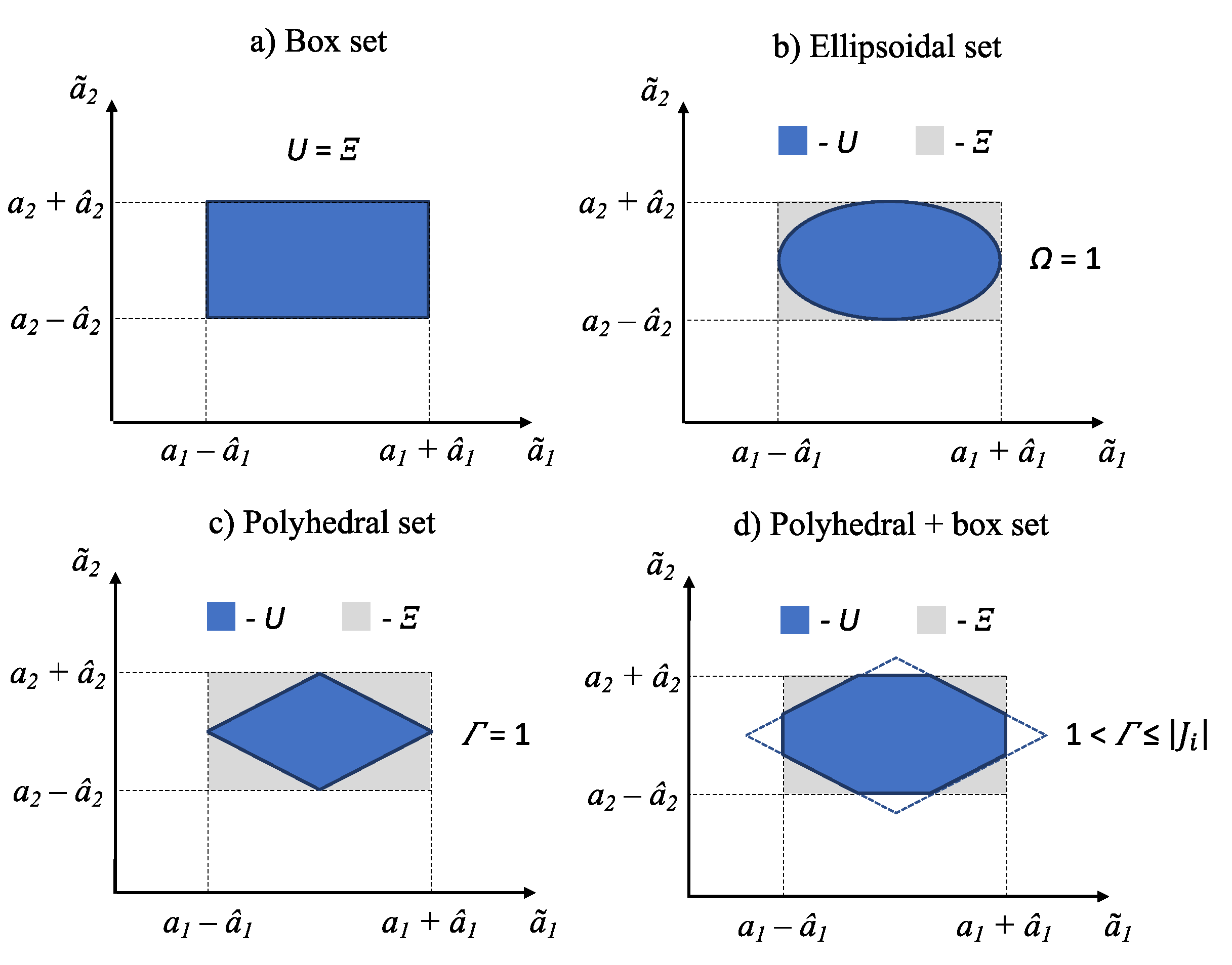
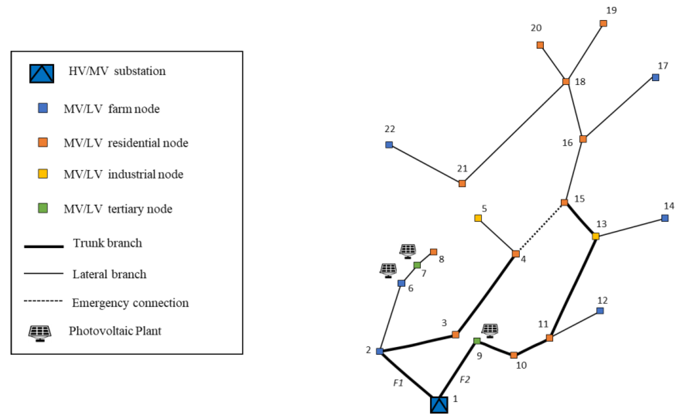
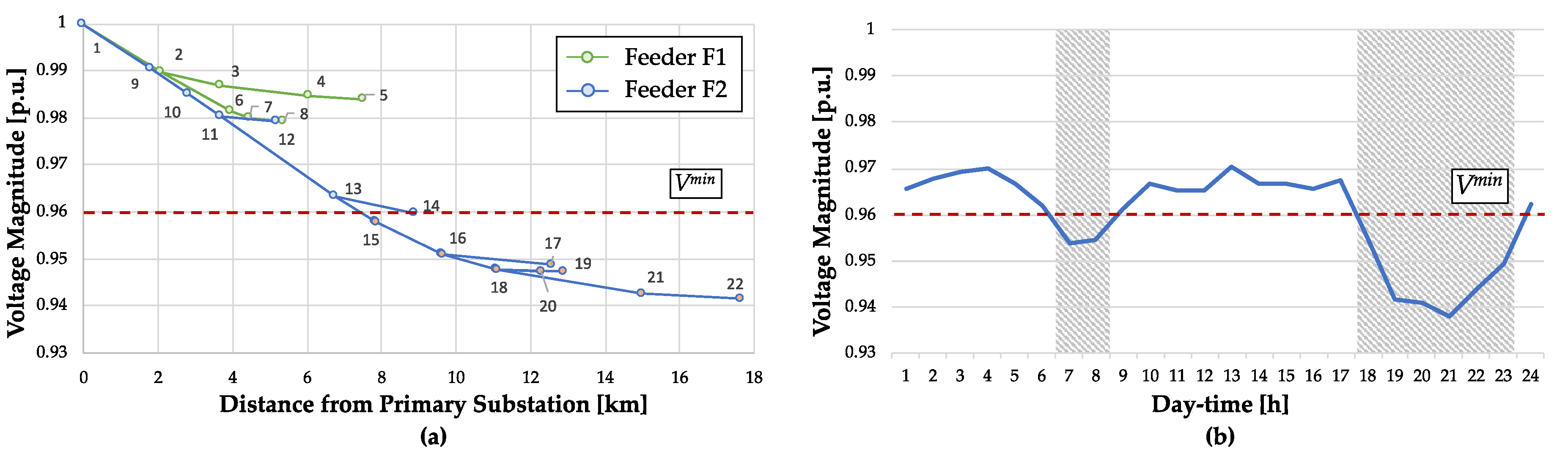
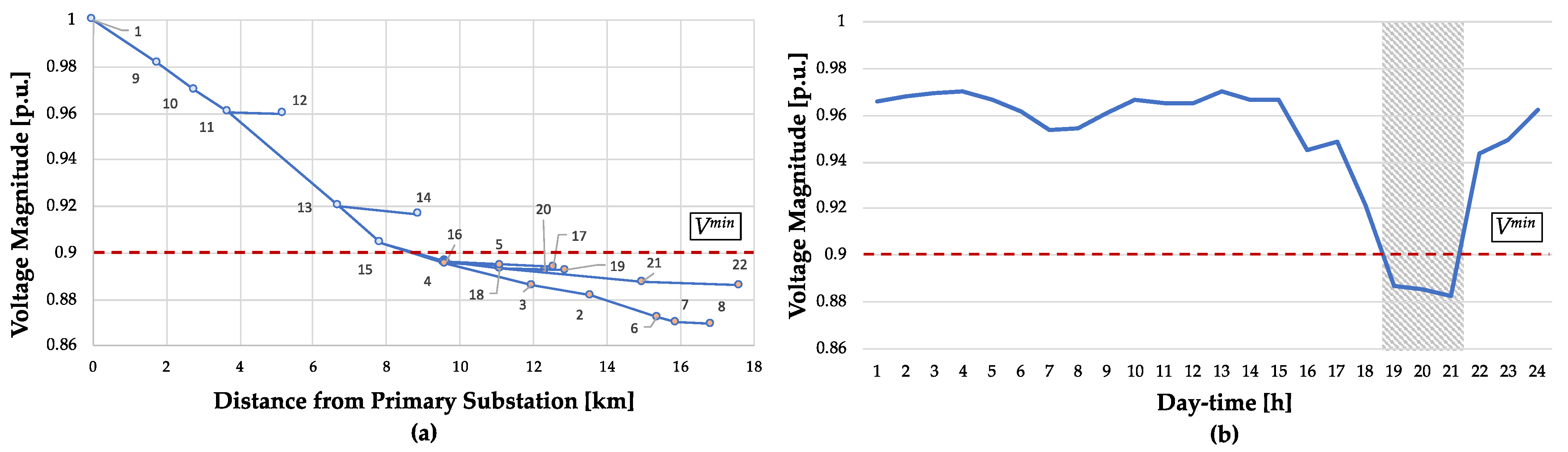
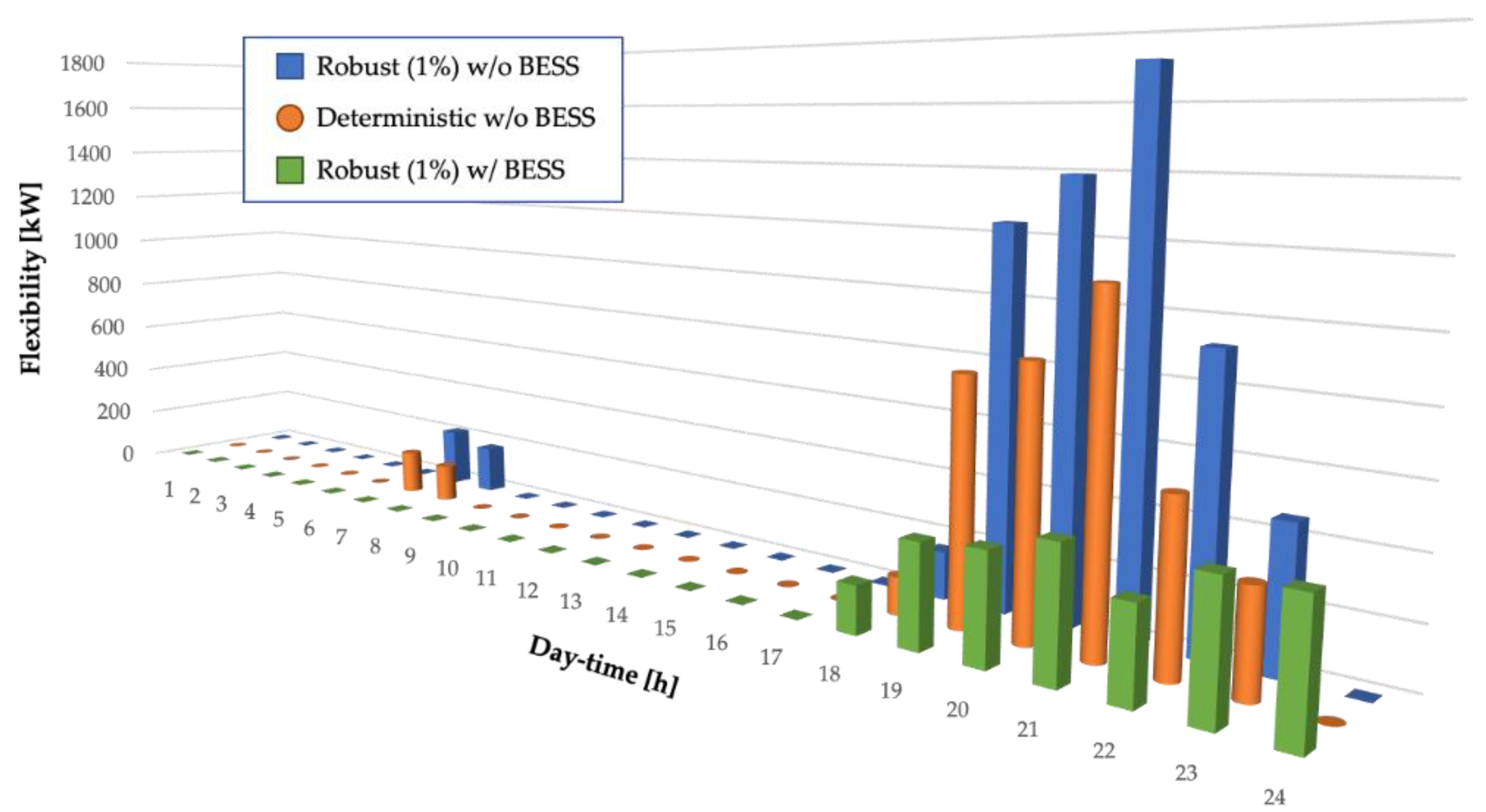