A Technique of Recursive Reliability-Based Missing Data Imputation for Collaborative Filtering

Abstract

Collaborative filtering (CF) is a recommendation technique that analyzes the behavior of various users and recommends the items preferred by users with similar preferences. However, CF methods suffer from poor recommendation accuracy when the user preference data used in the recommendation process is sparse. Data imputation can alleviate the data sparsity problem by substituting a virtual part of the missing user preferences. In this paper, we propose a k-recursive reliability-based imputation (k-RRI) that first selects data with high reliability and then recursively imputes data with additional selection while gradually lowering the reliability criterion. We also propose a new similarity measure that weights common interests and indifferences between users and items. The proposed method can overcome disregarding the importance of missing data and resolve the problem of poor data imputation of existing methods. The experimental results demonstrate that the proposed approach significantly improves recommendation accuracy compared to those resulting from the state-of-the-art methods while demanding less computational complexity.

1. Introduction

With the advance of Web-based technologies, there is a rapid growth in products and services available on online platforms leading to the information overload problem. As a result, manually searching and finding relevant products and services for a user have become challenging and time-consuming. Recommendation systems can alleviate the information overload problem, as they help platforms automatically locate the items that the users are most likely to consume with respect to their preferences. Thus, the recommendation systems have been successfully used in various commercial applications, such as movie recommendations on Netflix, book recommendations on Amazon, or music recommendations on Last.fm.

One of the most widely used recommendation techniques is collaborative filtering (CF), which analyzes the behavior of various users and recommends the items preferred by users with similar preferences. For example, a user may express preferences for an item through item rating, purchase behavior, and search behavior. The main idea of the CF method is that a group of users, who are interested in the same item, exhibit similar tendencies for other items, and the items that are selected together by the same user have a prerequisite that they are also selected by other users [1,2]. If a CF method only relies on the original user–item interaction, we call it a pure CF method [3]. The pure CF method can only provide satisfactory recommendations for users, considering that there are sufficient past interactions. However, in actual systems, the user is often restricted in expressing preferences for items. In other words, the number of evaluations of items is much smaller than that of the actual number of items selected. As a result, the pure CF methods suffer from poor recommendation accuracy due to insufficient user preference data. We can refer to this problem as a data sparsity problem.

Generally, the CF method is used in a variety of recommendation systems to predict the interests of users, including movie and music [4,5], travel routes [6,7], products [8,9,10], and online resources [11]. Various methods are proposed to solve the data sparsity problem in CF methods by substituting a virtual part of the nonexistent user preferences. For example, Ma et al. [12] proposed an Effective Missing Data Prediction (EMDP) method, which prioritizes high-reliability data for imputation and only imputes the missing data when it exceeds the predefined threshold. Other methods [13,14,15,16] incorporated the EMDP method into their proposed methods to solve a data sparsity problem in various fields. The main advantage of EMDP is that it can avoid poor imputation (no or insufficient amount of imputed data) because it imputes all the data whose similarities with the active user and active item exceed the thresholds. However, the main disadvantage of EMDP is a relatively poor accuracy because it gives the same value to all missing data [17]. On the other hand, Ren et al. [18,19,20,21] proposed the Auto-Adaptive Imputation (AutAI) and Adaptive Maximum imputation (AdaM) methods, which consider neighborhood information when imputing missing data. That is, AutAI and AdaM impute data of high importance by focusing on data rated by both users. Considering that the data imputed by AutAI and AdaM are highly important data containing most information on the prediction data, high accuracy can be maintained even with a small number of imputed missing data. However, the main limitation of these approaches is the risk of poor imputation, leading to no or insufficient imputed data in some cases, where the user’s rating history is much smaller than those of other users [22,23].

In this paper, we propose a k-recursive reliability-based imputation (k-RRI) for CF. The proposed method can overcome the disadvantage of EMDP of disregarding the importance of missing data and resolving the problem of poor data imputation of AutAI and AdaM. More specifically, we make the following contributions in this paper:

• We propose an effective method for missing data imputation that improves the poor recommendation accuracy of CF caused by the data sparsity problem. The proposed method, k-RRI, first selects data with high reliability and then recursively imputes data with additional selection while gradually lowering the reliability criterion. Existing methods replaced the data with a small amount of real data at once; however, we replaced the data with real and reliable virtual data to alleviate the data sparsity problem.
• We also propose a new similarity measure that weights common interests and indifferences between users and items. This enables us to determine the similarities between user and items more accurately.
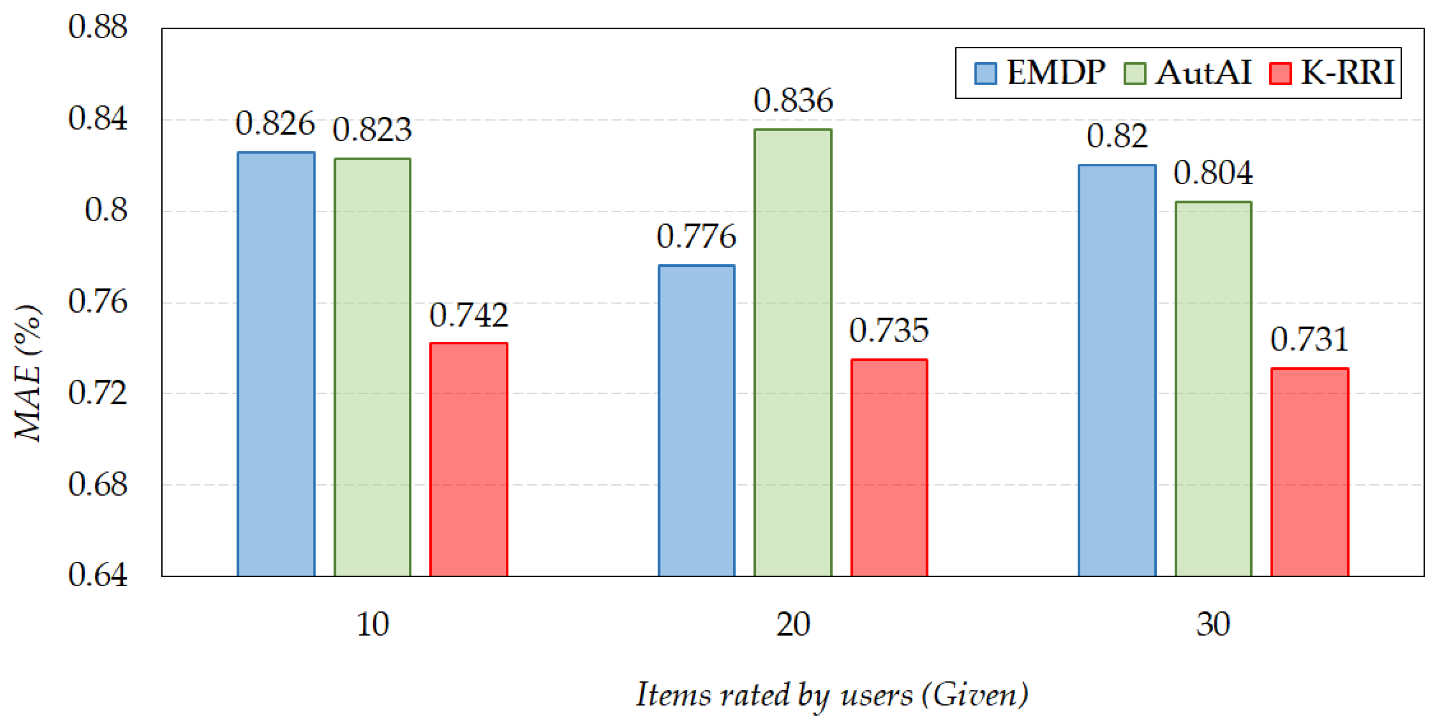
• We evaluated the performance of the proposed approach through experiments with state-of-the-art methods: EMDP and AutAI. The experimental results demonstrate that the proposed approach using a new similar measure significantly improves recommendation accuracy compared to those resulting from the state-of-the-art methods while demanding less computational complexity.

The rest of this paper is organized as follows. Section 2 explains the preliminaries for our work. Section 3 discusses related studies that solved the data sparsity problem in CF. Section 4 describes the proposed method in detail. Section 5 presents the result of the performance evaluation. Section 6 summarizes and concludes the paper.

2. Preliminaries

This section explains preliminaries for our work. In this paper, we focus on the neighborhood-based CF that can generally be divided into two steps: neighbor selection and rating combination. We first explain the similarity measure for neighbor selection in Section 2.1. Then, we elaborate the neighborhood-based rating prediction method in Section 2.2.

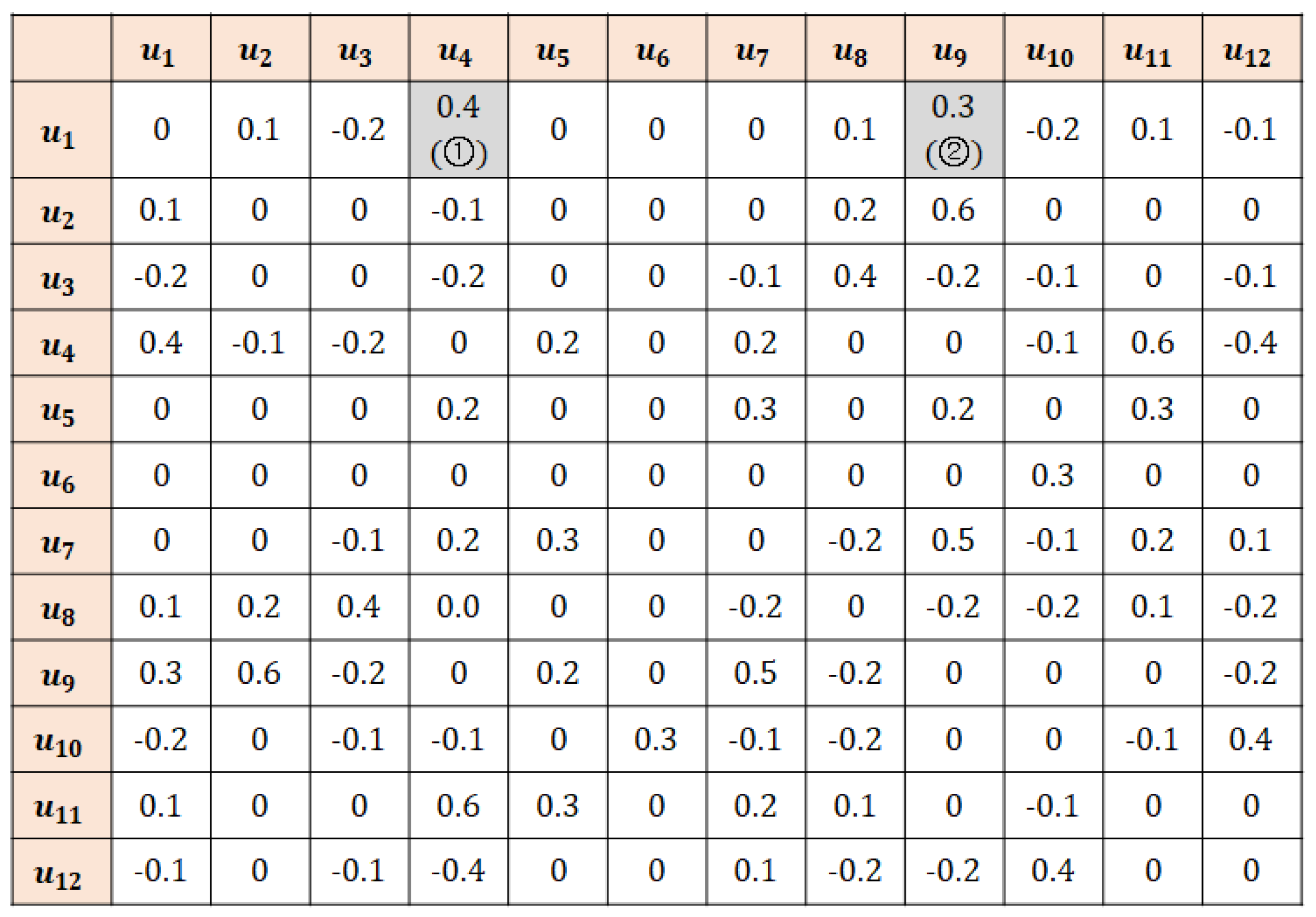
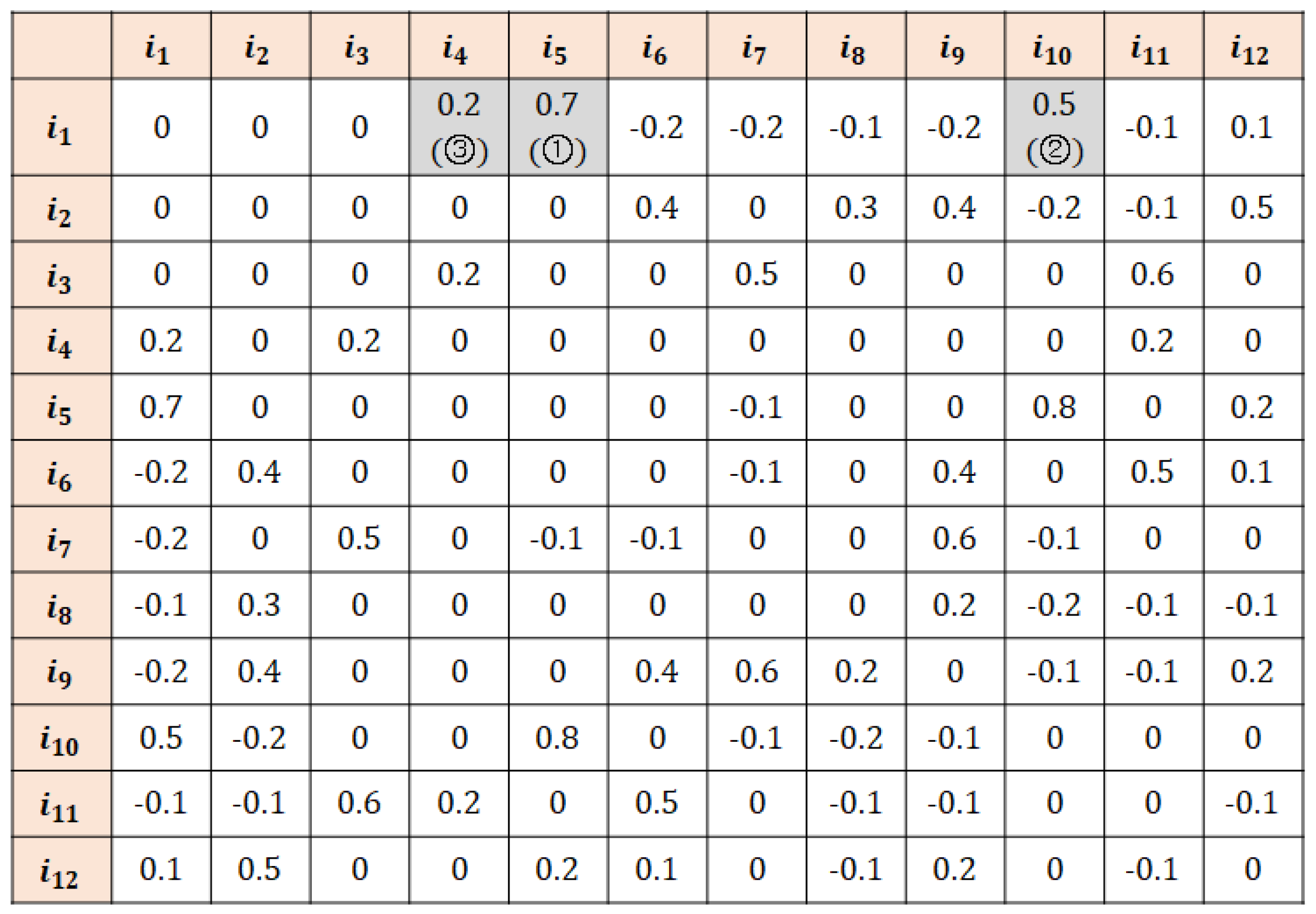
2.1. Similarity Measures

The process of neighborhood-based CF is characterized by defining similar users or items as neighbors and recommending items based on the rating histories of the selected neighbors. Thus, neighbor selection depends on the definition of similarity. The similarity measurements widely used in various fields include Pearson’s Correlation Coefficient, Cosine Similarity, and Jaccard Index. Pearson’s Correlation Coefficient compares the linear correlation between two variables. Cosine Similarity is a measure of the difference in orientation between two vectors, and Jaccard Index is a measure of similarity expressed as the ratio of the intersection of two sets to the size of their union. In this paper, we use Pearson’s Correlation Coefficient as the primary similarity measure, which is the most widely used measure in the field of CF [24].

The similarity between users $a$ and $b$ [$Si{m}_u\left(a,b\right)$] and that between items $s$ and $t$ [$Si{m}_i\left(s,t\right)$] are defined by Equations (1) and (2), respectively, where $I\left(a,b\right)$ is the intersection of the items rated by users $a$ and $b$, and $U\left(s,t\right)$ is the intersection of the users that rated the items $s$ and $t$; $\overline{r_a}$ and $\overline{r_b}$ are the average ratings given by users $a$ and $b$, respectively, and $\overline{r_s}$ and $\overline{r_t}$ are the average ratings received by items $s$ and $t$, respectively [24,25,26]. The denominator and numerator indicate the extent to which the ratings of two users and items change separately and together, respectively. The extent of change in user ratings can be calculated by adding up the squared deviations obtained by comparing all ratings pertaining to $I\left(a,b\right)$ with the average rating. Similarly, the extent of change in item ratings can be calculated by adding up the squared deviations obtained by comparing all ratings pertaining to $U\left(s,t\right)$ with the average rating. The similarity measure is a real number in the closed interval $\left[-1,1\right]$, whereby a higher value indicates a higher correlation. In general, if the Pearson’s correlation coefficient is greater than or equal to $0.1$, it indicates a positive correlation. If it is less than $-0.1$, it indicates negative correlation, and any value in the open interval $\left(-0.1,0.1\right)$ indicates no correlation.

$$Si{m}_u\left(a,b\right)=\frac{{\sum }_{i\in I\left(a,b\right)}\left(r_{a,i}-\overline{r_a}\right)\left(r_{b,i}-\overline{r_b}\right)}{\sqrt{{\sum }_{i\in I\left(a,b\right)}{\left(r_{a,i}-\overline{r_a}\right)}^2}\sqrt{{\sum }_{i\in I\left(a,b\right)}{\left(r_{b,i}-\overline{r_b}\right)}^2}}$$

(1)

$$Si{m}_i\left(s,t\right)=\frac{{\sum }_{u\in U\left(s, t\right)}\left(r_{u,s}-\overline{r_s}\right)\left(r_{u,t}-\overline{r_t}\right)}{\sqrt{{\sum }_{u\in U\left(s,t\right)}{\left(r_{u,s}-\overline{r_s}\right)}^2}\sqrt{{\sum }_{u\in U\left(s,t\right)}{\left(r_{u,t}-\overline{r_t}\right)}^2}}$$

(2)

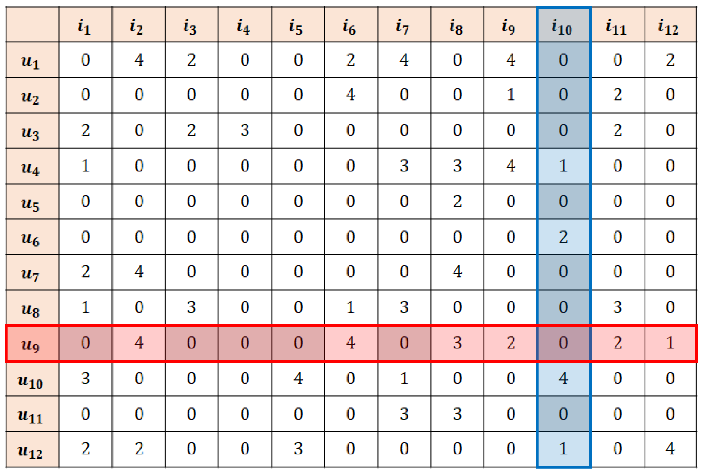
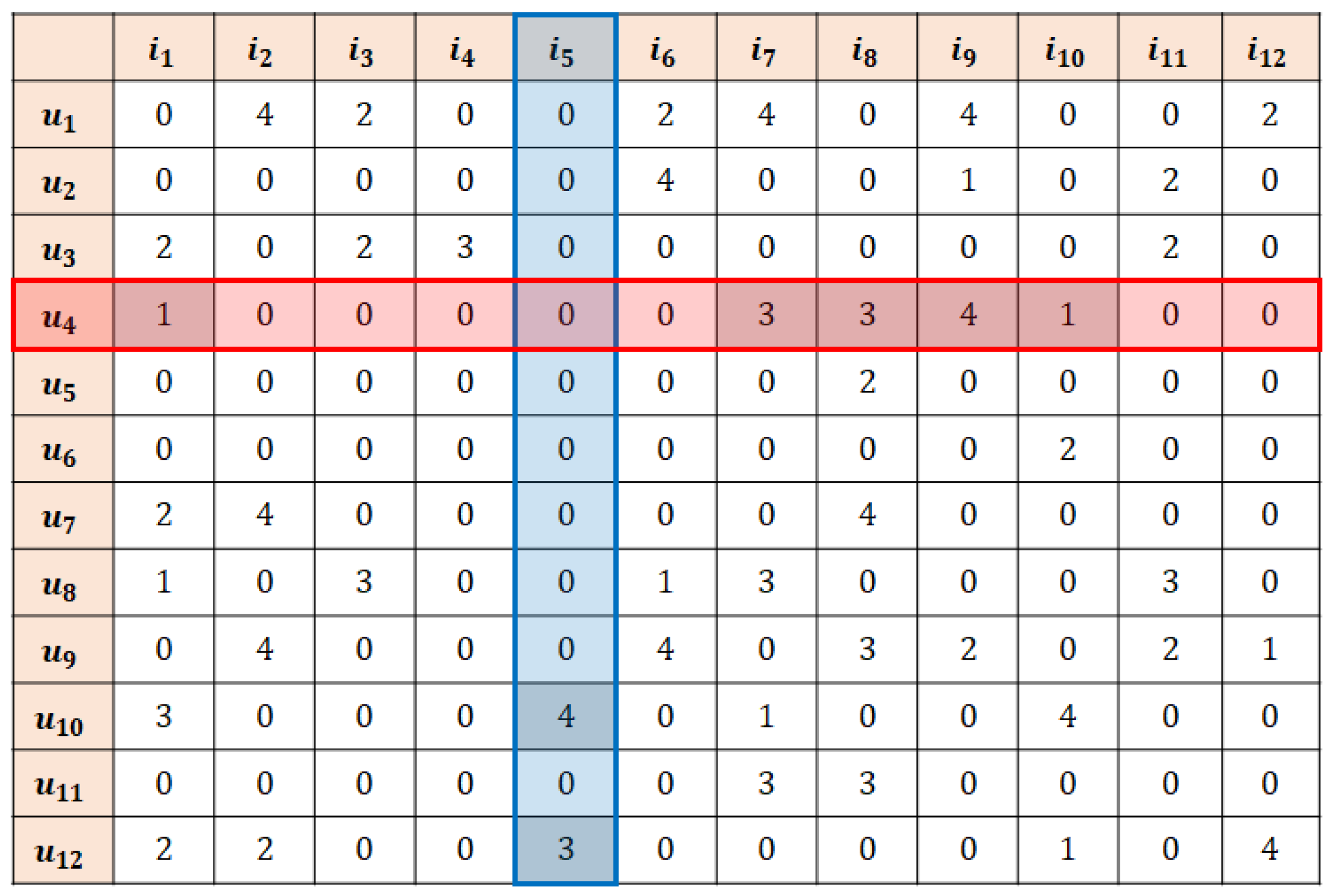
2.2. Rating Prediction Method

This section describes the method to predict user ratings for items in the neighborhood-based CF process. The predictions of user ratings for items can be divided into user-based and item-based predictions. User-based predictions are based on the target user’s ratings for other items and similar users’ ratings for the target item. The item-based prediction is based on the ratings that the target item has received from other users and the ratings that similar items have received from the target user.

User $a$’s neighbor $N_u\left(a\right)$ is defined as the set of $k$ users that have high similarities with $a$. Similarly, item $s$’s neighbor $N_i\left(s\right)$ is defined as the set of $k$ items that have high similarities with $s$. Equation (3) represents the rating of user $a$’s user-based prediction for item $s$, where $\overline{u_x}$ is the average rating of all item ratings from any given user $x$. Similarly, Equation (4) represents the rating of user $a$’s item-based prediction for item $s$, where $\overline{i_y}$ is the average rating of all user ratings for any given item $y$.

$${\widehat{r}}_{a,s}^u=\overline{u_a}+\frac{{\sum }_{x\in N_u\left(a\right)}Si{m}_u\left(a,x\right)\times \left(r_{x,s}-\overline{u_x}\right)}{{\sum }_{x\in N_u\left(a\right)}Si{m}_u\left(a,x\right)}$$

(3)

$${\widehat{r}}_{a,s}^i=\overline{i_s}+\frac{{\sum }_{y\in N_i\left(s\right)}Si{m}_i\left(s,x\right)\times \left(r_{a,y}-\overline{i_y}\right)}{{\sum }_{y\in N_i\left(s\right)}Si{m}_i\left(s,y\right)}$$

(4)

The rating for item $s$ predicted by user $a$ [${\widehat{r}}_{a,s}$] can be obtained by combining user $a$’s user-based and item-based rating predictions for item $s$ $[{\widehat{r}}_{a,s}^u$] in Equation (3) and $[{\widehat{r}}_{a,s}^i$] in Equation (4), respectively, using the parameter $\lambda$, as expressed by Equation (5). Here, $\lambda$ is a real number in the closed interval $\left[0,1\right]$. Specifically, $\lambda =0$ and $\lambda =1$ represent the item-based and user-based predictions, respectively, as the user-based prediction is offset to zero by the coefficient value $\lambda$ and the item-based prediction is offset to zero by the coefficient value $\left(1-\lambda \right)$ [18,19].

$${\widehat{r}}_{a,s}=\lambda {\widehat{r}}_{a,s}^u+\left(1-\lambda \right){\widehat{r}}_{a,s}^i$$

(5)

Recall from Section 1 that if a CF method only relies on the original user–item interaction, we call it a pure CF method [3]. Generally, the pure CF method can achieve high efficiency in recommendation tasks. However, when users rarely express their preferences for items, it is difficult for pure CF methods to gather the required amount of user preference data for the recommendation. In other words, most pure CF methods suffer from poor recommendation accuracy when the user preference data used in the recommendation process is sparse. We refer to this problem as a data sparsity problem. In the next section, we discuss the studies that solved the data sparsity problem using EMDP, AutAI and AdaM methods.

3. Related Studies

In this section, we review related studies. We can roughly classify these studies into the following three categories: (1) studies that use the CF method in various fields; (2) studies that solve the data sparsity problem with EMDP method; and (3) studies that solve the data sparsity problem with AutAI and AdaM methods.

Due to its simplicity and ease of implementation, the CF-based methods are used in a variety of recommendation systems to predict the interests of users. For example, Musa et al. [4] proposed a CF approach for efficient movie recommendations using two similarity measures: item–item correlation and item–item adjusted cosine similarity. Cohen et al. [5] proposed a method that improves the efficiency of music recommendations by integrating data collected from the web into user ratings. Logesh et al. [6] proposed a personalized recommender system that considers users’ activities, behaviors, and relationships between them in predicting Points of Interest (POIs) travel recommendations. Logesh et al. [7] also proposed integrating user’s contextual information, i.e., opinion mining from textual reviews and posts, into personalized recommender systems to provide efficient recommendations to the tourists. Similar work was also performed by Zhao et al. [8,9], where the authors proposed a product recommendation system that considers internal user factors, i.e., user sentimental deviations and the review’s reliability. Recently, an artificial intelligence-based product recommendation approach, called Neural Interactive Collaborative Filtering, was proposed by Zou et al. [10]. The authors used an efficient Q-learning mechanism to solve the cold-start and warm-start recommendation problems. Chen et al. [11] proposed a personalized recommendation method for online video learning resources using an association rule mining mechanism to discover helpful videos for students.

There were several methods to solve the data sparsity problem. For example, Ma et al. [11] proposed an Effective Missing Data Prediction (EMDP) method, which prioritizes high-reliability data for imputation and defines imputation data as data with similarity exceeding the threshold. Here, the similarity is computed using the equation proposed by Herlocker [27], which is based on the modified Pearson’s Correlation Coefficient. Considering that the Pearson’s Correlation Coefficient determines similarity based on datasets of items rated by both users, its reliability decreases if the number of the rated items is small. Therefore, a higher weight is assigned to larger data size. That is, when the Pearson’s Correlation Coefficient values are identical, the data with a larger intersection size is considered to have a higher similarity. In other words, by adding weight to the similarity measure in EMDP, we can lower the similarity value obtained from a dataset with a small number of items rated by both users. Equation (6) for user–user similarity computation is the result of adding this weight to Equation (1), where $\left|I_a\cap I_b\right|$ is the number of items rated by both users. In the same manner, the item–item similarity is obtained by adding this weight to Equation (2), as expressed by Equation (7), where $\left|U_s\cap U_t\right|$ is the number of users that rated both items. Here, parameters $\gamma$ and $\delta$ are input values for user similarity and item similarity, respectively, and the computed similarity value of an item rated by both users is defined to be reliable only when it is larger than or equal to $\gamma$ and $\delta$. Accordingly, when weight is assigned to $Si{m}_u^{\prime }\left(a,b\right)$, the lower value between $\left|I_a\cap I_b\right|$ and $\gamma$ is taken as the numerator and is divided by the denominator $\gamma$ to prevent $Si{m}_u^{\prime }\left(a,b\right)$ from exceeding $1$, as per the basic definition of similarity. The same applies to the weight of $Si{m}_i^{\prime }\left(s,t\right)$: the lower value between $\left|U_s\cap U_t\right|$ and $\delta$ is taken as the numerator and is divided by the denominator $\delta$ to prevent $Si{m}_i^{\prime }\left(s,t\right)$ from exceeding $1$. For example, in the case of the parameter value $\gamma$ = 10, if the number of items rated by both users is 10 or more, then $Si{m}_u^{\prime }\left(a,b\right)=Si{m}_u\left(a,b\right)$. If the number of items rated by both users is 5, then $Si{m}_u^{\prime }\left(a,b\right)=\frac{1}{2}Si{m}_u\left(a,b\right)$, and half of the computed similarity value is taken. As the value of $\gamma$ increases, the number of items rated by both users exerts higher influence on the similarity value, whereby it is always equal to or lower than the value computed with Equation (1). Similarly, as the value of $\delta$ increases, the number of users that rated both items exerts higher influence on the similarity value, whereby it is always equal to or lower than the value computed from Equation (2).

$$Si{m}_u^{\prime }\left(a, b\right)=\frac{Min\left(\left|I_a\cap I_b\right|, \gamma \right)}{\gamma }\times Si{m}_u\left(a,b\right)$$

(6)

$$Si{m}_i^{\prime }\left(s, t\right)=\frac{Min\left(\left|U_s\cap U_t\right|, \delta \right)}{ \delta }\times Si{m}_i\left(s,t\right)$$

(7)

There were several methods that solved a data sparsity problem based on EMDP in various fields. For example, Özbal et al. [13] proposed to solve the data sparsity problem in movie recommendation applications by combining EMDP and Local and Global User Similarity (LU&GU) [28] methods. These approaches were improved by integrating the content information of the movies (e.g., cast, director, genre) during the item similarity calculations. The experiment results showed that the overall system performance improved when the proposed method was augmented with content information. Agarwal and Bharadwaj et al. [14] proposed a CF method for friend recommendation based on their interaction intensity and adaptive user similarity in social networks. To solve the data sparsity problem, the authors incorporated EMDP into the proposed method. As a result, the proposed method with EMDP outperformed its variants on a sparse dataset. Shin et al. [15] proposed a content-aware CF for expert recommendation in social networks. The proposed method uses a new cosine similarity measure, where a weight is assigned for the local similarities among users. By using this similarity measure, the authors predicted missing values based on EMDP and formed a preference score prediction table, where experts are selected with the highest scores. The experiment results demonstrated that the proposed method outperforms the traditional content-aware CF method. Inan et al. [16] proposed to combine EMDP with a method proposed by Özbal et al. [13] to achieve more efficient movie recommendations. Similar to [13], the proposed method was integrated with content information of the movies during the item similarity calculations. In addition, the authors used a goal programming technique to calculate the movie feature’s similarity scores. The experiment results of the proposed method showed that it outperforms existing methods when it uses content information with a goal programming technique. The main advantage of EMDP is that it can avoid poor imputation (no or insufficient amount of imputed data) because it imputes all the data whose similarities with the active user and active item exceed the thresholds. However, the main disadvantage of EMDP is a relatively poor accuracy because it gives the same value to all missing data [17].

According to a study by Cover [29] on the nearest neighbor rule, the nearest neighbor of a data point in an infinite training dataset shares over 50% of the information with that data point. In other words, when predicting a value, neighboring data have information values of different importance. Ren et al. [18,19] proposed the Auto-Adaptive Imputation (AutAI) method, which considers neighborhood information when imputing missing data. AutAI imputes data of high importance by focusing on data rated by both users. In AutAI, the data to be imputed are defined as the dataset combining the items rated by one or more neighboring users among the items rated by the active user and the users who rated one or more neighboring items among the users who rated the active item. The main feature of AutAI is that it can operate with any similarity measure, and it outperforms existing neighborhood-based CF approaches. Ren et al. [20,21] also proposed an improvement of the AutAI method, which is called an Adaptive Maximum imputation (AdaM). The main idea of the AdaM is to maximize the imputation advantage and minimize the imputation error. To achieve the maximum imputation, the authors proposed determining the imputation area from both the user and the item perspectives. As a result, there is at least one real rating guaranteed for each item in the determined imputation area so as to avoid misleading analysis caused by the imputation error. The experiment results showed that the AdaM outperforms the existing methods owing to more accurate neighbor identification. As the data imputed by AutAI and AdaM are highly important data containing most information on the prediction data, high accuracy can be maintained even with a small number of imputed missing data. However, the main limitation of these approaches is the risk of poor imputation, leading to no or insufficient imputed data in some cases, where the active user’s rating history is much smaller than those of other users [22,23].

4. k-Recursive Reliability-Based Imputation (k-RRI)

This section is devoted to a new imputation method, k-RRI. We first describe k-RRI in Section 4.1. Then, we explain a stepwise reliability-based threshold reset process of the proposed method in Section 4.2. Lastly, we analyze a computational complexity of k-RRI and compare it with those of EMDP and AutAI in Section 4.3.

4.1. k-RRI

In this paper, we propose a k-RRI, which is a recursive imputation method for CF based on reliability. We first define the related key terms used in this paper as follows:

• Active user: the user of the data targeted for prediction.
• Active item: the item of the data targeted for prediction.
• Key neighbors: a set of data necessary for predicting the active user and the active item. Each imputation algorithm will define the key neighbors and impute the missing data, i.e., unrated data, among them.
• High-reliability data: a set of data whose similarity with the active user and active item exceeds the given threshold.

According to the prerequisite for neighborhood-based CF defined by [17], the similar nearest neighbor has the most information regarding the data to be predicted. Accordingly, k-RRI is implemented according to the criteria defined below.

• Definition 1: Missing data are selectively imputed in a stepwise and decreasing order of reliability.
• Definition 2: Data imputed in the preceding step can be used for imputation in the succeeding step.
• Definition 3: The threshold cutoff value decreases as the algorithm progresses. That is, the reliability-based threshold cutoff criteria are strict in earlier recursive steps and become increasingly relaxed toward the end.

Similarity is determined by the Herlocker’s modified similarity computation equation [27] presented in Section 2, whereby the number of data unrated by both users is included in the weight. In other words, in the case of the identical Pearson’s Correlation Coefficient, the larger the size of the unrated data subset, the higher the similarity. In k-RRI, the user–user similarity is defined by Equation (8), which is a modification of Equation (1) by incorporating a weight factor. The purpose of adding weight to the similarity measure in k-RRI is to lower the similarity value obtained in cases where there are only a small number of data rated or unrated by both users. In Equation (8), $\left|I_a^c\cap I_b^c\right|$ is the number of items that have not been rated by both users. In the same manner, the item–item similarity is defined by Equation (9), which is a modification of Equation (2) by adding a weight factor. In Equation (9), $\left|U_s^c\cap U_t^c\right|$ is the number of the users who have not rated both items. Parameters ${\gamma }_I$ and ${\gamma }_{I^c}$ are required as input values when computing user similarity with the k-RRI algorithm, whereby a user similarity value is considered reliable only if the number of the data rated by both users is higher than or equal to ${\gamma }_I$ and the number of the data unrated by both users is higher than or equal to ${\gamma }_{I^c}$. Thus, when assigning weight to $Si{m}_u^{\prime }\left(a,b\right)$, the lower values between $\left|I_a\cap I_b\right|$ and ${\gamma }_I$ and between $\left|I_a^c\cap I_b^c\right|$ and ${\gamma }_{I^c}$ are taken as the numerator and divided by the product of ${\gamma }_I$ and ${\gamma }_{I^c}$ to prevent $Si{m}_u^{\prime }\left(a,b\right)$ from exceeding $1$, as per the basic definition of similarity. Similarly, a user similarity value is considered reliable only if the number of data rated by both users is higher than or equal to ${\delta }_U$ and the number of the data unrated by both users is higher than or equal to ${\delta }_{U^c}$. Accordingly, when assigning weight to $Si{m}_u^{\prime }\left(s,t\right)$, the lower values between $\left|U_s\cap U_t\right|$ and ${\delta }_U$ and between $\left|U_s^c\cap U_t^c\right|$ and ${\delta }_{U^c}$ are taken as the numerator and divided by the product of ${\delta }_U$ and ${\delta }_{U^c}$ to prevent $Si{m}_u^{\prime }\left(s,t\right)$ from exceeding $1$. For example, in the case of the parameter values ${\gamma }_I=10$ and ${\gamma }_{I^c}=20$, if the number of items rated by both users is 10 or more and the number of the items unrated by both users is 20 or more, then $Si{m}_u^{\prime }\left(a,b\right)=Si{m}_u\left(a,b\right)$. However, if the number of items unrated by both users is 5 but the number of the items rated by both users is 10, then $Si{m}_i^{\prime }\left(s,t\right)=\frac{1}{4}Si{m}_i\left(s,t\right)$, where one-quarter of the computed similarity value is taken. As the value of ${\gamma }_I$ increases, the number of items rated by both users exerts a higher influence on the similarity value. In addition, as the value of ${\gamma }_{I^c}$ increases, the number of items unrated by both users exerts a higher influence on the similarity value, whereby it is always equal to or lower than the value computed from Equation (1). Similarly, as the value of ${\delta }_U$ increases, the number of users that rated both items exerts higher influence on the similarity value, and as the value of ${\delta }_{U^c}$ increases, the number of users that have not rated both items exerts a higher influence on the similarity value, whereby it is always equal to or lower than the value computed from Equation (2).

$$Si{m}_u^{\prime }\left(a, b\right)=\frac{Min\left(\left|I_a\cap I_b\right|, {\gamma }_I\right)}{{\gamma }_I}\times \frac{Min\left(\left|I_a^c\cap I_b^c\right|,{\gamma }_{I^c}\right)}{{\gamma }_{I^c}}\times Si{m}_u\left(a,b\right)$$

(8)

$$Si{m}_i^{\prime }\left(s, t\right)=\frac{Min\left(\left|U_s\cap U_t\right|, {\delta }_U\right)}{{\delta }_U}\times \frac{Min\left(\left|U_s^c\cap U_t^c\right|, {\delta }_{U^c}\right)}{{\delta }_{U^c}}\times Si{m}_i\left(s,t\right)$$

(9)

The basic steps of the k-RRI are described in Algorithm 1. The input values for Algorithm 1 are the user–item rating matrix, user–item similarity set, active user and active item for prediction, number of recursive steps, and final user and item similarity thresholds. The output is the imputed matrix for the active user and the active item. In Algorithm (1), the final user similarity threshold ${\eta }_k$ is used when selecting a high-reliability user set. The user similarity threshold at any given step $[{\eta }_r$] is a value between 1 (i.e., maximum similarity value) and ${\eta }_k$. Similarly, the final item similarity threshold ${\theta }_k$ is used when selecting a high-reliability item set, and the item similarity threshold at any given step $[{\theta }_r$] is a value between 1 (i.e., maximum similarity value) and ${\theta }_k$. ${\eta }_k$ and ${\theta }_k$ indicate any real number in the closed interval $\left[0,1\right]$, which is the similarity range. In the first line, the imputed matrix is initialized with the user–item rating matrix. Lines 2–13 represent the process of imputing missing data according to the threshold cutoff value, which is reset at each iteration while performing the $k$ recursive steps. As the algorithm progresses, the threshold cutoff values are decreased. In the third line, the current user and item similarity thresholds (${\eta }_r$ and ${\theta }_r$, respectively) are set. The reliability-based threshold reset process for determining ${\eta }_r$ and ${\theta }_r$ is explained in detail in Section 4.2. The sets of users ${\mathcal{U}}_a$ and items ${ℐ}_s$ satisfying the current threshold values are generated in lines 4 and 5, respectively. In line 6, the key neighbor set ${\mathcal{N}}_{a,s}$ is selected, combining the elements of ${\mathcal{U}}_a$ and ${ℐ}_s$. That is, ${\mathcal{N}}_{a,s}$ is the set of data containing information necessary for predicting user $u_a$’s rating of item $i_s$. In lines 7–12, the imputed matrix is filled by imputing the missing values among the elements of ${\mathcal{N}}_{a,s}$. ${\widehat{r}}_{a^{\prime }{s}^{\prime }}$ in the ninth line is calculated using the rating prediction method described in Section 2.2.

Algorithm 1: k-RRI
Input:	the user–item rating matrix $ℛ$.
	the similarity set $si{m}^{\prime }$.
	the active user $u_a$. the active item $i_s$.
	the number of steps $k$.
	the user’s final similarity threshold ${\eta }_k$.
	the item’s final similarity threshold ${\theta }_k$.
Output:	the imputed matrix ${ℛ}^{\prime }$.
1:	${ℛ}^{\prime }\leftarrow ℛ$; // initialize the imputed matrix
2:	for$r\leftarrow 1$until$k$do
3:	calculate ${\eta }_r$, ${\theta }_r$;
4:	${\mathcal{U}}_a\leftarrow \left\{u_{a^{\prime }}| {\eta }_r<si{m}^{\prime }\left(u_{a^{\prime }},u_a\right)\le {\eta }_{r-1},u_{a^{\prime }}\ne u_a\right\}$;
5:	${ℐ}_s\leftarrow \left\{i_{s^{\prime }}| {\theta }_r<si{m}^{\prime }\left(i_{s^{\prime }},i_s\right)\le {\theta }_{r-1},i_{s^{\prime }}\ne i_s\right\}$;
6:	${\mathcal{N}}_{a,s}\leftarrow \left\{r_{a^{\prime }{s}^{\prime }}|u_{a^{\prime }}\in {\mathcal{U}}_a\vee i_{s^{\prime }}\in {\mathcal{T}}_s\right\}$;
7:	for each $r_{a^{\prime }{s}^{\prime }}\in {\mathcal{N}}_{a,s}$ do
8:	if $r_{a^{\prime }{s}^{\prime }}=\mathsf{\varnothing }$ then
9:	calculate ${\widehat{r}}_{a^{\prime }{s}^{\prime }}$;
10:	${ℛ}^{\prime }\left(u_{a^{\prime }},i_{s^{\prime }}\right)\leftarrow {\widehat{r}}_{a^{\prime }{s}^{\prime }}$;
11:	end if
12:	end for
13:	end for

Example. Figure 1 and Figure 2 show the user and item similarity matrices, respectively, where $u_1$ and $i_1$ are the active user and active item, respectively, which are computed by the similarity measure employed by the k-RRI algorithm. Let the number of k-RRI steps be set at $k=3$ and the user threshold values in steps 1–3 be ${\eta }_1=0.3$, ${\eta }_2=0.2$, and ${\eta }_3=0.1$, respectively. Then, the set of users ${\mathcal{U}}_1$ selected in step 1 is $\left\{u_4\right\}$ because its similarity with the active user $u_1$ exceeds threshold ${\eta }_1=0.3$. Similarly, let the item threshold values in steps 1–3 be ${\theta }_1=0.6$, ${\theta }_2=0.3$, and ${\theta }_3=0.1$. Then, the set of the items ${ℐ}_1$ selected in step 1 is $\left\{i_5\right\}$ because its similarity with the active item $i_1$ exceeds ${\theta }_1=0.6$. Accordingly, the ratings that $\left\{u_4\right\}$ gives to all items and the ratings that $\left\{i_5\right\}$ receives from all users become the set of key neighbors ${\mathcal{N}}_{1,1}$ in step 1. The missing data to be imputed are the unrated values among the key neighbors (the parts marked in Figure 3).

On the other hand, the set of users ${\mathcal{U}}_1$ selected in step 2 $is\left\{u_9\right\}$, whose similarity with the active user $u_1$ is between threshold ${\eta }_2=0.2$ and ${\eta }_1=0.3$, and the set of items ${ℐ}_1$ is $\left\{i_{10}\right\}$, whose similarity with the active item $i_1$ is between threshold ${\theta }_2=0.3$ and ${\theta }_1=0.6$. Accordingly, the ratings that $\left\{u_9\right\}$ gives to all items and the ratings that $\left\{i_{10}\right\}$ receives from all users become the set of key neighbors ${\mathcal{N}}_{1,1}$ in step 2. The missing data to be imputed are the unrated values among the key neighbors (the parts marked in Figure 4).

Lastly, the set of users ${\mathcal{U}}_1$ selected in step 3 is $\mathsf{\varnothing }$, whose similarity with the active user $u_1$ is between threshold ${\eta }_3=0.1$ and ${\eta }_2=0.2$, and the set of items ${ℐ}_1$ is $\left\{i_4\right\}$, whose similarity with the active item $i_1$ is between threshold ${\theta }_3=0.1$ and ${\theta }_2=0.3$. Accordingly, the ratings that $\left\{i_4\right\}$ receives from all users become the set of key neighbors ${\mathcal{N}}_{1,1}$ in step 3, and the missing data to be imputed are the unrated values among the key neighbors (the parts marked in Figure 5).

4.2. Threshold Reset Process

Unlike EMDP and AutAI, k-RRI uses a recursive algorithm with stepwise iteration, whereby the final imputation matrix can vary depending on the recursive structure. The imputation error can be defined as an error incurred by imputing an empty dataset with an arbitrary value. In k-RRI, missing data are imputed in a given step based on the actual rating histories and the virtual data imputed in the preceding step. Therefore, not only does the imputation error affect the step concerned, but it is also carried forward to the next step, as expressed by Equation (10), where $k$ is the number of recursive steps, ${\epsilon }_r$ is the imputation error incurred in the $r$-th step, and ${\alpha }_i$ and ${\beta }_i$ are constants.

$$\begin{gathered} {\epsilon }_2={\alpha }_1{\epsilon }_1+{\beta }_1 \\ {\epsilon }_3={\alpha }_2{\epsilon }_2+{\beta }_2={\alpha }_2\left({\alpha }_1{\epsilon }_1+{\beta }_1\right)+{\beta }_2={\alpha }_1{\alpha }_2{\epsilon }_1+{\beta }_1{\beta }_2 \\ ⋮ \\ {\epsilon }_k={\alpha }_1{\alpha }_2\cdots {\epsilon }_1+{\beta }_1{\beta }_2\cdots {\beta }_k \end{gathered}$$

(10)

Owing to the recursive nature of the proposed algorithm, the propagation of imputation errors is inevitable; however, minimization of initial imputation errors can prevent much of the error propagation. In each step, care should be taken to select and impute only high-reliability data. Equations (11) and (12) represent the user and item similarity thresholds, respectively, of the reliability-based threshold cutoff values in the $r$-th step, where $\eta$ and $\theta$ denote the final user and item similarity thresholds, respectively. As the algorithm progresses, ${\eta }_r$ and ${\theta }_r$ decrease, while the value of $r$ increases. For example, let $\eta =0.7$ and $k=3$; then, the threshold will have values as follows: ${\eta }_1=0.93$, ${\eta }_2=0.85$, and ${\eta }_3=0.70$, whereby the deviation increases from $-0.08$ between ${\eta }_1$ and ${\eta }_2$ to $-0.15$ between ${\eta }_2$ and ${\eta }_3$. Therefore, by setting strict cutoff criteria in earlier steps, reliable data are left as imputation candidate data in later steps. Further into the algorithmic process, the cutoff criterion becomes increasingly relaxed. This threshold cutoff reset method contributes to minimizing the propagation imputation errors that occur when imputing data from low-reliability candidate data.

$${\eta }_r=1-\frac{\left(1-\eta \right)\times 2^r}{2^k}$$

(11)

$${\theta }_r=1-\frac{\left(1-\theta \right)\times 2^r}{2^k}$$

(12)

4.3. Comparison of Computational Complexity

The purpose of this study is to enhance prediction accuracy; however, it is important to note that the dependence of computational complexity on the system size is also a significant factor. The benefit obtained by high prediction accuracy can be offset by a higher computational complexity, rendering the algorithm uncompetitive in a practical setting. Therefore, we conducted a theoretical comparison of EMDP, AutAI, and k-RRI with a focus on the computational complexity.

Three imputation algorithms presented in this paper, namely EMDP, AutAI, and k-RRI, can generally be divided into the following process parts:

• Key neighbor selection stage: selection of the key neighbors of interest.
• Missing data imputation stage [30]: identification of the missing data from the key neighbors and implementation of missing data imputation.

Equations (13)–(15) represent the computational complexities of EMDP, AutAI, and k-RRI, respectively, where $M$ and $N$ denote the total numbers of users and items, respectively.

$$\begin{array}{cc}\hfill tim{e}_{EMDP}& =tim{e}_{key neighbor selection}+tim{e}_{missing data imputation}\hfill \\ & =O\left(MN\right)+O\left({\mathcal{N}}_{EMDP}\right)\\ & =O\left(MN+{\mathcal{N}}_{EMDP}\right)\\ & =O\left(MN\right)\end{array}$$

(13)

$$\begin{array}{cc}\hfill tim{e}_{AutAI}& =tim{e}_{key neighbor selection}+tim{e}_{missing data imputation}\hfill \\ & =O\left(MN\right)+O\left({\mathcal{N}}_{AutAI}\right)\\ & =O\left(MN+{\mathcal{N}}_{AutAI}\right)\\ & =O\left(MN\right)\end{array}$$

(14)

$$\begin{array}{cc}\hfill tim{e}_{k-RRI}& =\left(tim{e}_{key neighbor selection}+tim{e}_{missing data imputation}\right)\times k\hfill \\ & =\left(O\left(\frac{1}{2}{M}^2+\frac{1}{2}{N}^2+MN\right)+O\left({\mathcal{N}}_{k-RRI}\right)\right)\times k\\ & =O\left(k\left(\frac{1}{2}{M}^2+\frac{1}{2}{N}^2+MN\right)\right)+O\left(k{\mathcal{N}}_{k-RRI}\right)\\ & =O\left(M^2+N^2+MN\right)+O\left({\mathcal{N}}_{k-RRI}\right)\\ & =O\left(max(M^2, N^2\right))+O\left({\mathcal{N}}_{k-RRI}\right)\\ & =O\left(max(M^2, N^2\right)+{\mathcal{N}}_{k-RRI})\\ & =O\left(max(M^2, N^2\right))\end{array}$$

(15)

In the key neighbor selection stage, all elements of the user–item rating matrix should be identified, of which the computational complexity is $O\left(MN\right)$. EMDP and AutAI implement this stage once, and k-RRI repeats it $k$ times at each iteration, with the user–item rating data changing every time. Changes in the user–item rating data entail changes in the user and item similarities. Therefore, k-RRI updates the similarity matrix at every iteration. Here, the time required for updating the user similarity matrix is $O\left(\frac{1}{2}{M}^2\right)$ and for the item similarity matrix is $O\left(\frac{1}{2}{N}^2\right)$. The number of recursive steps $k$ is a negligibly small constant irrespective of the numbers of users and items; thus, it can be disregarded in terms of big-O notation. Accordingly, the computational complexity of k-RRI in the key neighbor selection stage is $O\left(k\left(\frac{1}{2}{M}^2+\frac{1}{2}{N}^2+MN\right)\right)=O\left(max(M^2,N^2)\right)$.

In the missing data imputation stage, all key neighbors are identified. Considering the characteristics of each algorithm, the numbers of key neighbors can be expressed by ${\mathcal{N}}_{AutAI}\le {\mathcal{N}}_{EMDP}\approx {\mathcal{N}}_{k-RRI}\ll MN$. That is, the computational complexity in the imputation stage is $O\left({\mathcal{N}}_{AutAI}\right)$, $O\left({\mathcal{N}}_{EMDP}\right)$, and $O\left({\mathcal{N}}_{k-RRI}\right)$, with the maximum time requirement being $O\left(MN\right)$. Given that the key neighbor selection stage is the dominant part in all three algorithms, the overall computational complexity is $O\left(MN\right)$ for EMDP and AutAI, and $O\left(max(M^2,N^2\right))$ for k-RRI. For similar user and item data sizes, the overall computational complexity of all three algorithms is $O\left(MN\right)$. This suggests that in a system with similar user and item data sizes, only prediction accuracy plays a role in algorithm selection.

5. Performance Evaluation

This section describes a performance comparison of the proposed k-RRI with EMDP and AutAI, which are two conventional imputation algorithms. Their performance accuracies are experimentally tested with a focus on prediction accuracy.

5.1. Experimental Setup

We used the MovieLens 1M Dataset provided by the University of Minnesota, which is widely used to test the performance of recommender systems. This dataset contains one million ratings from 6000 users on 4000 items. For the purpose of performance testing, we extracted 500 users from the MovieLens 1M Dataset, generated a training dataset, and labeled it $M_{500}$. The test dataset was generated by extracting another 500 users. To assume data sparsity conditions, items rated by the test dataset users were provided in limited numbers of 10, 20, and 30, which are labeled as $Give{n}_{10}$, $Give{n}_{20}$, and $Give{n}_{30}$. This is an experimental setup mostly used to test the performance of recommender systems.

The performance of an imputation algorithm should be evaluated by the final ratings predicted by the algorithm rather than its interim products. To maintain consistency with other studies, we applied the Mean Absolute Error (MAE) as a metric to compare the algorithms [31,32]. Equation (16) is an equation for calculating MAE, where $r_{as}$ and ${\widehat{r}}_{as}$ are the real and predicted ratings, respectively, by user $u_a$ on item $t_s$, $X$ is the test dataset, and $\left|X\right|$ is the size of $X$. The lower the value of MAE, the higher the prediction accuracy. Its value can be any real number ranging from 0 to 5 as the MovieLens 1M Dataset uses ratings from 1 to 5.

$$\mathit{M}\mathit{A}\mathit{E}=\frac{{\sum }_{\left(\mathit{a},\mathit{s}\right)\in \mathit{X}}\left|{\mathit{r}}_{\mathit{a}\mathit{s}}-{\widehat{\mathit{r}}}_{\mathit{a}\mathit{s}}\right|}{\left|\mathit{X}\right|}.$$

(16)

Prior to the implementation of the imputation algorithm, the values of the parameters provided by each imputation algorithm must be defined. To avoid research bias problems, we employed the values used in other studies [12]. More specifically, the parameters of EMDP and k-RRI were set at $\lambda =0.7$, $\gamma =30$, $\delta =25$, and $\eta =\theta =0.4$, and those of AutAI were set at $\lambda =0.4$ and $k=10$.

5.2. Experimental Results

Figure 6 shows the results of comparing the prediction accuracies of the EMDP, AutAI, and k-RRI algorithms for the training datasets $M_{500}Give{n}_{10}$, $M_{500}Give{n}_{20}$, and $M_{500}Give{n}_{30}$.

From the graph, we can observe that the MAE scores of EMDP and AutAI for the $M_{500}Give{n}_{10}$ dataset were 0.826 and 0.823, respectively, indicating that AutAI slightly outperformed EMDP. For the $M_{500}Give{n}_{10}$ dataset, the highest accuracy was shown by the proposed method k-RRI, outperforming EMDP by 11.3% and AutAI by 10.9%. On the other hand, the MAE scores of EMDP and AutAI for the $M_{500}Give{n}_{20}$ dataset were 0.776 and 0.836, respectively, indicating that EMDP outperformed AutAI. For $M_{500}Give{n}_{20}$, the highest accuracy was shown by the proposed method k-RRI, outperforming EMDP by 5.6% and AutAI by 13.8%. Lastly, the MAE scores of EMDP and AutAI for $M_{500}Give{n}_{30}$ dataset were 0.820 and 0.804, respectively, indicating that AutAI slightly outperformed EMDP. As in the previous two cases, the highest accuracy was shown by k-RRI, outperforming EMDP by 12.2% and AutAI by 10.0%.

Figure 7 demonstrates the results of comparing the prediction accuracies of k-RRI as the number of k values varies. From the graph, we can observe that the highest accuracy can be obtained when the number of k values is set to $k=8$ for the $M_{500}Give{n}_{10}$ and $M_{500}Give{n}_{20}$ datasets, and $k=6$ for the $M_{500}Give{n}_{30}$ dataset. It is important to note that the prediction accuracy of k-RRI varied depending on the number of recursive steps with standard deviation (SD), which is a measure of the variation or dispersion of a dataset. The SD exhibited values of 0.0047, 0.0048, and 0.0022 at $Give{n}_{10}$, $Give{n}_{20}$, and $Give{n}_{30}$, respectively. The SD may be significantly high or negligibly low depending on the system’s characteristics. From this perspective, $k$ = 2 is recommended for a system less sensitive to prediction accuracy in terms of computational time. For a system sensitive to prediction accuracy, it is recommended that the value of $k$ should be optimized according to the system under consideration.

6. Conclusions

In this paper, we have proposed an effective imputation method for missing data to improve the poor recommendation accuracy due to data sparsity in CF. The proposed method, k-RRI, is a recursive imputation method based on reliability. We have also proposed a new similarity measure that weights common interests and indifferences between users and items. As a result, the proposed k-RRI has achieved the following advantages over existing methods: (1) poor imputation can be avoided because the threshold values are adjusted depending on the reliability level required in each step; (2) the importance of missing data is reflected in imputation because priority is given to the nearest neighbors with important information on the data to be predicted; and (3) a sufficient number of candidate data for imputation can be ensured because the data imputed in the preceding step are used in each step. We compared the prediction accuracy of k-RRI with EMDP and AutAI through the experiments, using the benchmark dataset, MovieLens. Experimental results show that the prediction accuracy of k-RRI outperforms existing methods by 13.8%.

As for the future work, we are planning to improve the processing time of k-RRI by developing an efficient neighbor searching method according to the reliability. We are also planning to study an algorithm that automatically determines parameters such as the number of steps, the similarity threshold, and so on. Furthermore, we are planning to incorporate the trust constraint into the proposed method in the future work as trust-awareness can also alleviate the data sparsity problem and further improve the accuracy of our method. Lastly, we are planning to apply the proposed method in various fields. For example, airplane services can greatly benefit from the proposed method considering that achieving high recommendation accuracy in airplane services is essential to satisfy customers.

References

1. Adomavicius, G.; Tuzhilin, A. Toward the Next Generation of Recommender Systems: A Survey of the State-of-the-Art and Possible Extensions. IEEE Trans. Knowl. Data Eng. 2015, 17, 734–749. [Google Scholar] [CrossRef]
2. Rendle, S.; Krichene, W.; Zhang, L.; Anderson, J. Neural Collaborative Filtering vs. Matrix Factorization Revisited. In Proceedings of the ACM Conference on Recommender Systems, Rio de Janeiro, Brazil, 22–26 September 2020; pp. 240–248. [Google Scholar]
3. Wang, Q.; Yin, H.; Wang, H.; Nguyen, Q.V.H.; Huang, Z.; Cui, L. Enhancing Collaborative Filtering with Generative Augmentation. In Proceedings of the 25th ACM SIGKDD International Conference on Knowledge Discovery & Data Mining, Anchorage, AK, USA, 4–8 August 2019; pp. 548–556. [Google Scholar]
4. Musa, J.M.; Zhihong, X. Item Based Collaborative Filtering Approach in Movie Recommendation System Using Different Similarity Measures. In Proceedings of the 6th International Conference on Computer and Technology Applications, Antalya, Turkey, 14–16 April 2020; pp. 31–34. [Google Scholar]
5. Cohen, W.W.; Fan, W. Web-collaborative filtering: Recommending music by crawling the web. Comput. Netw. 2000, 33, 685–698. [Google Scholar] [CrossRef]
6. Logesh, R.; Subramaniyaswamy, V. Exploring hybrid recommender systems for personalized travel applications. Cogn. Inform. Soft Comput. 2019, 768, 535–544. [Google Scholar]
7. Logesh, R.; Subramaniyaswamy, V.; Vijayakumar, V.; Li, X. Efficient user profiling based intelligent travel recommender system for individual and group of users. Mob. Netw. Appl. 2019, 24, 1018–1033. [Google Scholar] [CrossRef]
8. Zhao, G.; Lei, X.; Qian, X.; Mei, T. Exploring users’ internal influence from reviews for social recommendation. IEEE Trans. Multimed. 2018, 21, 771–781. [Google Scholar] [CrossRef]
9. Zhao, G.; Lou, P.; Qian, X.; Hou, X. Personalized location recommendation by fusing sentimental and spatial context. Knowl. Based Syst. 2020, 196, 105849. [Google Scholar] [CrossRef]
10. Zou, L.; Xia, L.; Ding, Z.; Song, J.; Liu, W.; Yin, D. Reinforcement learning to optimize long-term user engagement in recommender systems. In Proceedings of the 25th ACM SIGKDD International Conference on Knowledge Discovery & Data Mining, Anchorage, AK, USA, 4–8 August 2019; pp. 2810–2818. [Google Scholar]
11. Chen, X.; Deng, H. Research on Personalized Recommendation Methods for Online Video Learning Resources. Appl. Sci. 2021, 11, 1–11. [Google Scholar]
12. Ma, H.; King, I.; Lyu, M.R. Effective missing data prediction for collaborative filtering. In Proceedings of the ACM SIGIR International Conference on Theory of Information Retrieval, Amsterdam, The Netherlands, 23–27 July 2007; pp. 39–46. [Google Scholar]
13. Özbal, G.; Karaman, H.; Alpaslan, F.N. A content-boosted collaborative filtering approach for movie recommendation based on local and global similarity and missing data prediction. Comput. J. 2011, 54, 1535–1546. [Google Scholar] [CrossRef]
14. Agarwal, V.; Bharadwaj, K.K. A collaborative filtering framework for friends recommendation in social networks based on interaction intensity and adaptive user similarity. Soc. Netw. Anal. Min. 2013, 3, 359–379. [Google Scholar] [CrossRef]
15. Shin, Y.S.; Kim, H.I.; Chang, J.W. A content-aware expert recommendation scheme in social network services. In Advanced Multimedia and Ubiquitous Engineering; Springer: Singapore, 2016; Volume 393, pp. 45–54. [Google Scholar]
16. Inan, E.; Tekbacak, F.; Ozturk, C. Moreopt: A goal programming based movie recommender system. J. Comput. Sci. 2018, 28, 43–50. [Google Scholar] [CrossRef]
17. Dong, J.; Tang, R.; Lian, G. Cooperative Filtering Program Recommendation Algorithm Based on User Situations and Missing Values Estimation. In Proceedings of the International Conference on Intelligent Information Processing, Guilin, China, 12–15 October 2018; pp. 247–258. [Google Scholar]
18. Ren, Y.; Zhang, J.; Zhou, W. The Efficient Imputation Method for Neighborhood-based Collaborative Filtering. In Proceedings of the 21st ACM International Conference on Information and Knowledge Management, Maui, HI, USA, 29 October–2 November 2012; pp. 684–693. [Google Scholar]
19. Ren, Y.; Li, G.; Zhang, J.; Zhou, W. Lazy collaborative filtering for data sets with missing values. IEEE Trans. Cybern. 2013, 43, 1822–1834. [Google Scholar] [CrossRef]
20. Ren, Y.; Li, G.; Zhang, J.; Zhou, W. AdaM: Adaptive-maximum imputation for neighborhood-based collaborative filtering. In Proceedings of the 2013 IEEE/ACM International Conference on Advances in Social Networks Analysis and Mining, New York, NY, USA, 25–28 August 2013; pp. 628–635. [Google Scholar]
21. Ren, Y.; Li, G.; Zhang, J.; Zhou, W. The maximum imputation framework for neighborhood-based collaborative filtering. Soc. Netw. Anal. Min. 2014, 4, 207. [Google Scholar] [CrossRef]
22. Suganeshwari, G.; Ibrahim, S.S. Rule-based effective collaborative recommendation using unfavorable preference. IEEE Access 2020, 8, 128116–128123. [Google Scholar] [CrossRef]
23. Lee, Y.; Kim, S.W.; Park, S.; Xie, X. How to Impute Missing Ratings? Claims, Solution, and Its Application to Collaborative Filtering. In Proceedings of the 20th International Conference on World Wide Web, New York, NY, USA, 28 March–1 April 2018; pp. 783–792. [Google Scholar]
24. Ahmadian, S.; Afsharchi, M.; Meghdadi, M. A novel approach based on multi-view reliability measures to alleviate data sparsity in recommender systems. Multimed. Tools Appl. 2019, 78, 17763–17798. [Google Scholar] [CrossRef]
25. Chae, D.K.; Kim, J.; Chau, D.H.; Kim, S.W. AR-CF: Augmenting Virtual Users and Items in Collaborative Filtering for Addressing Cold-Start Problems. In Proceedings of the 43rd International ACM SIGIR Conference on Research and Development in Information Retrieval, New York, NY, USA, 11–15 July 2020; pp. 1251–1260. [Google Scholar]
26. Margaris, D.; Spiliotopoulos, D.; Karagiorgos, G.; Vassilakis, C. An Algorithm for Density Enrichment of Sparse Collaborative Filtering Datasets Using Robust Predictions as Derived Ratings. Algorithms 2020, 13, 174. [Google Scholar] [CrossRef]
27. Herlocker, J.; Konstan, J.A.; Riedl, J. An empirical analysis of design choices in neighborhood-based collaborative filtering algorithms. Inf. Retr. 2002, 5, 287–310. [Google Scholar] [CrossRef]
28. Luo, H.; Nju, C.; Shen, R.; Ullrich, C. A collaborative filtering framework based on both local user similarity and global user similarity. Mach. Learn. 2008, 72, 231–245. [Google Scholar] [CrossRef] [Green Version]
29. Cover, T. Estimation by the nearest neighbor rule. IEEE Trans. Inf. Theory 1968, 14, 50–55. [Google Scholar] [CrossRef] [Green Version]
30. Mohammadi, F.; Zheng, C. A precise SVM classification model for predictions with missing data. In Proceedings of the 4th National Conference on Applied Research in Electrical, Mechanical Computer and IT Engineering, Tehran, Iran, 4 October 2018. [Google Scholar]
31. Wang, W.; Lu, Y. Analysis of the Mean Absolute Error (MAE) and the Root Mean Square Error (RMSE) in Assessing Rounding Model. Mater. Sci. Eng. 2018, 324, 012049. [Google Scholar] [CrossRef]
32. Nguyen, L.V.; Hong, M.S.; Jung, J.J.; Sohn, B.S. Cognitive Similarity-Based Collaborative Filtering Recommendation System. Appl. Sci. 2020, 10, 4183. [Google Scholar] [CrossRef]
Figure 1. An example of user similarity matrix of k-RRI.
Applsci 11 03719 g001
Figure 2. An example of item similarity matrix of k-RRI.
Applsci 11 03719 g002
Figure 3. An example of missing data imputation of k-RRI.
Applsci 11 03719 g003
Figure 4. An example of missing data imputation of k-RRI (step 2).
Applsci 11 03719 g004
Figure 5. An example of missing data imputation of k-RRI (step 3).
Applsci 11 03719 g005
Figure 6. The prediction accuracy of missing data imputation algorithms.
Applsci 11 03719 g006
Figure 7. The prediction accuracy of k-RRI as number of k values varies.
Applsci 11 03719 g007
Publisher’s Note: MDPI stays neutral with regard to jurisdictional claims in published maps and institutional affiliations.