
Groundwater Quality Monitoring Using In-Situ Measurements and Hybrid Machine Learning with Empirical Bayesian Kriging Interpolation Method

 ,
,  ,
,  ,
,
Abstract
:Featured Application
Abstract
1. Introduction
2. Materials and Methods
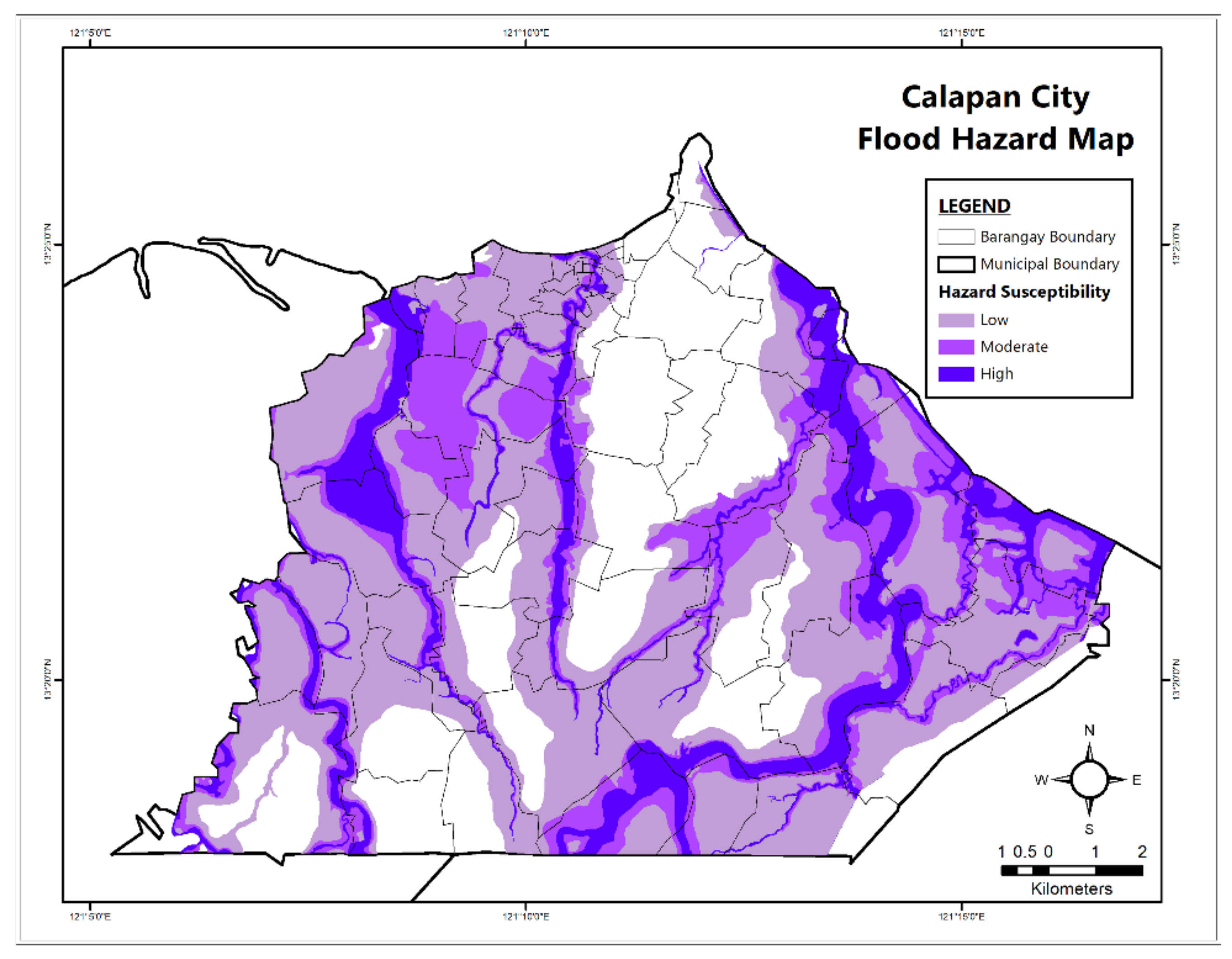
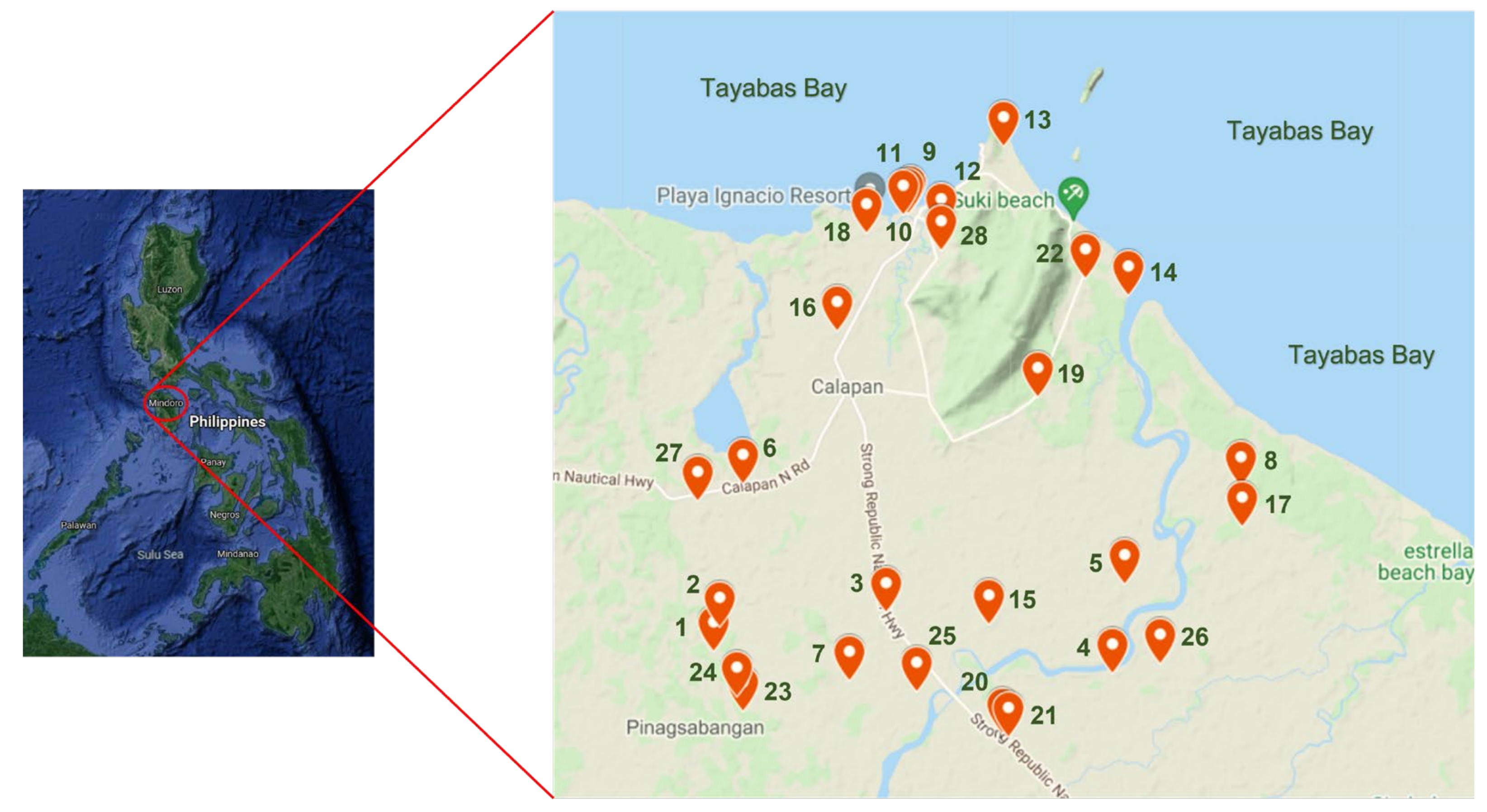
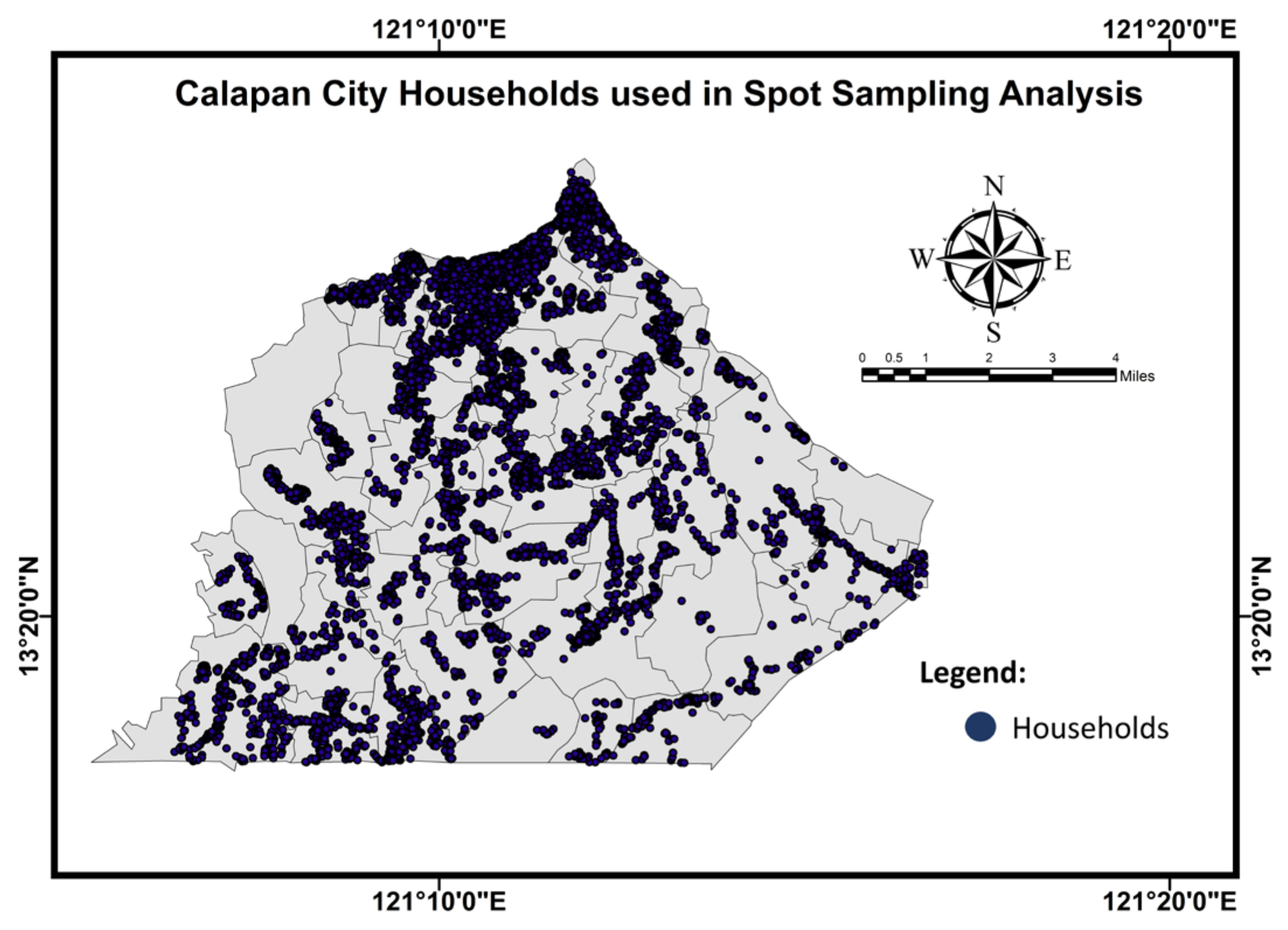
2.1. Description of the Study Area
2.2. Collection/Treatment of Groundwater Samples
2.3. Physicochemical and Metal Concentrations Analysis
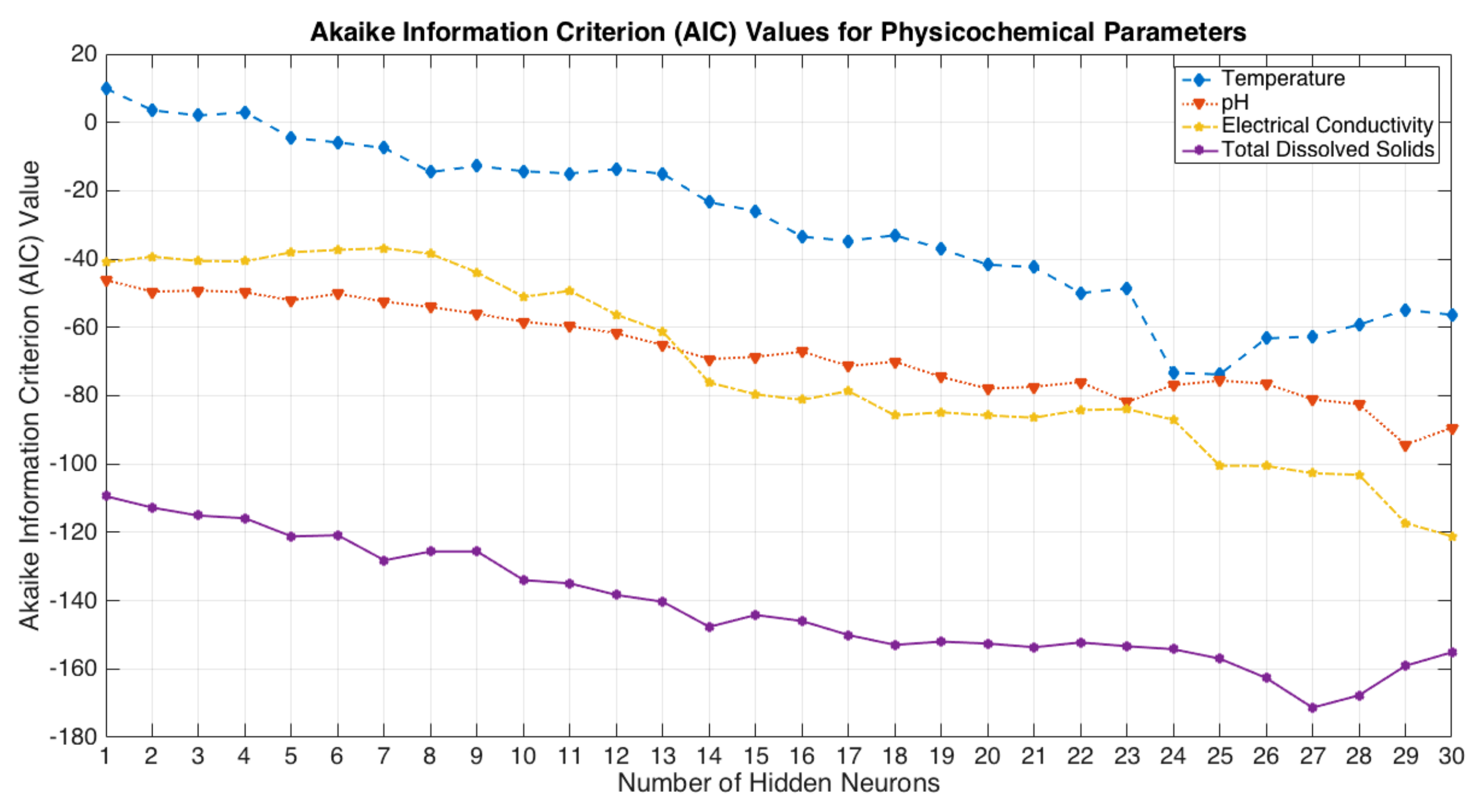
2.4. Spatial Concentration Mapping Using Machine Learning Informed Empirical Bayesian Kriging (EBK) Method
3. Results
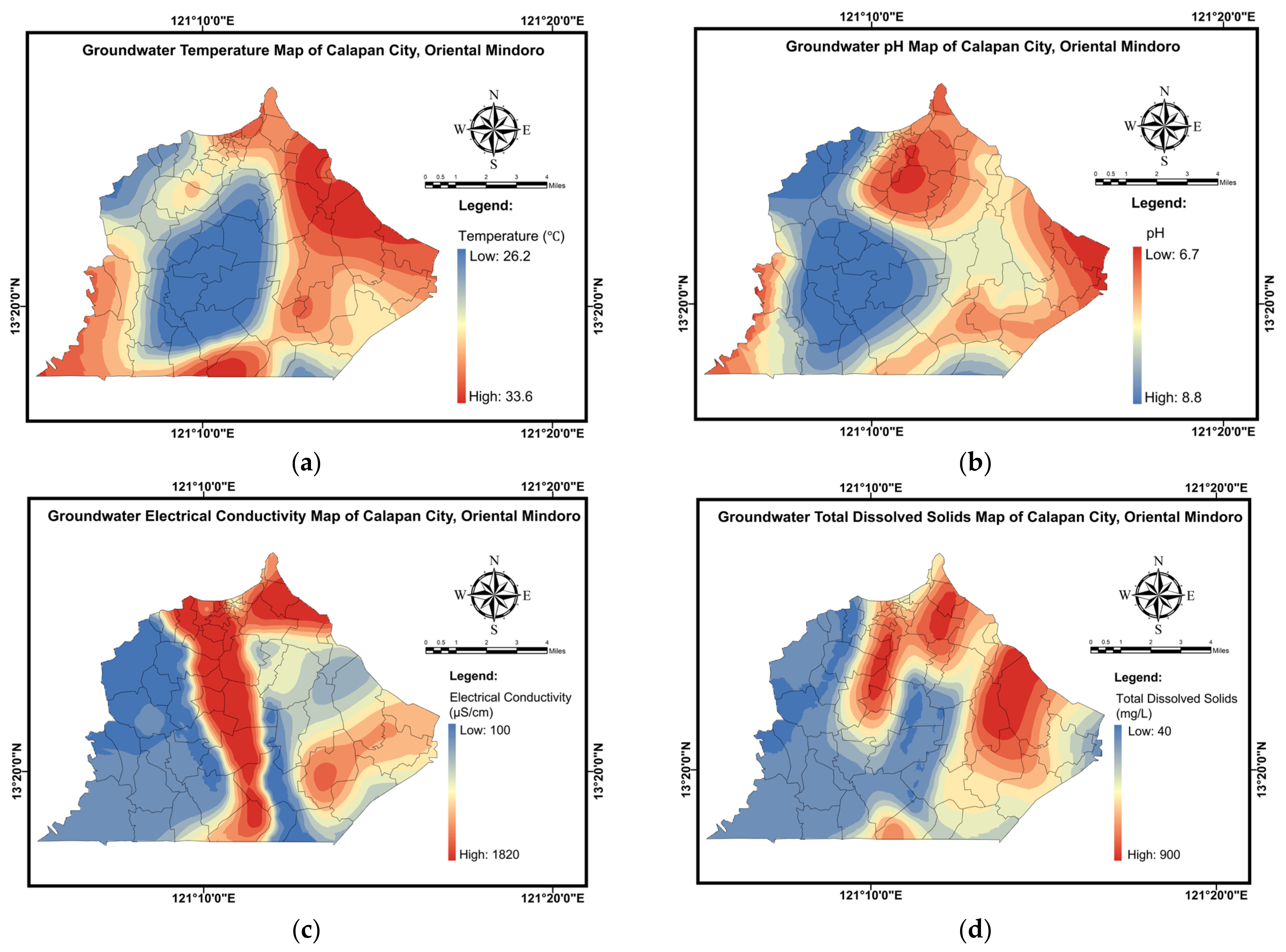
3.1. Physicochemical Groundwater Parameters
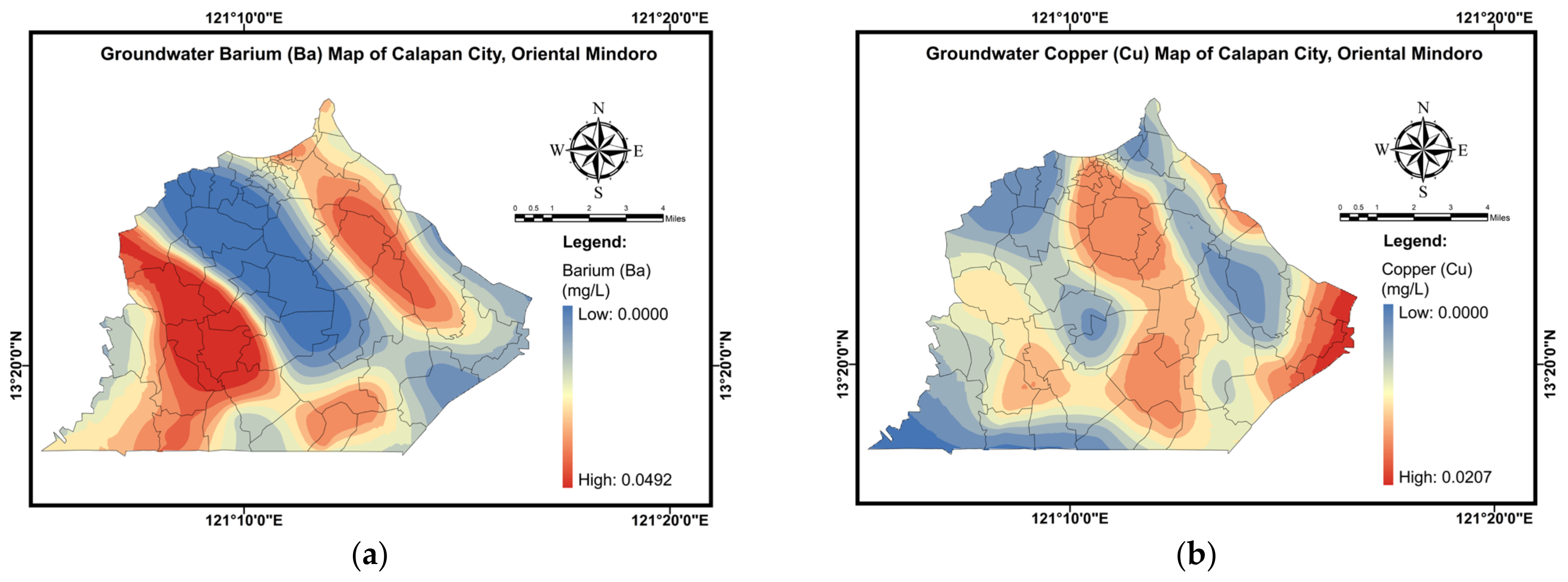
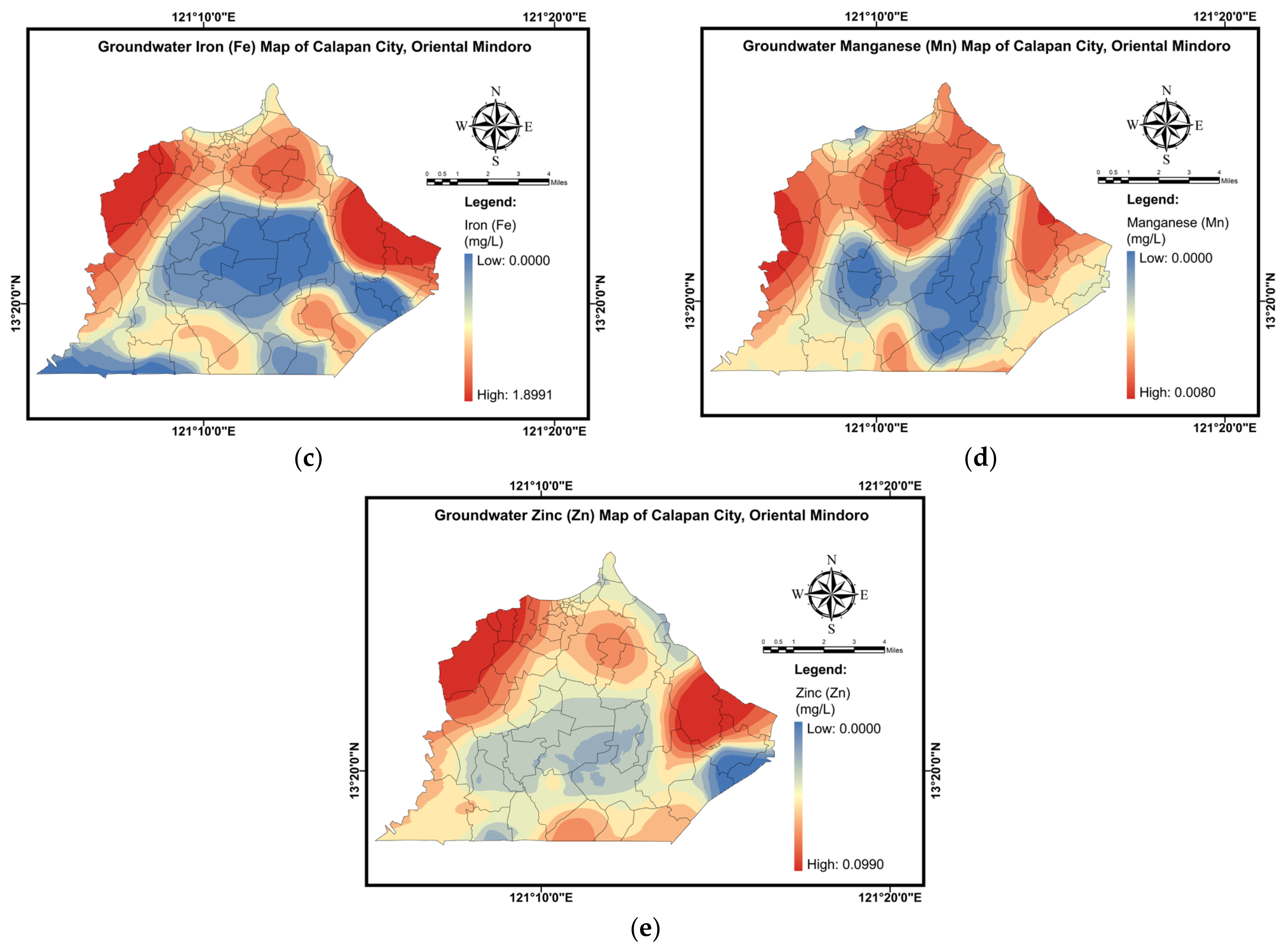
3.2. Heavy Metal Concentrations
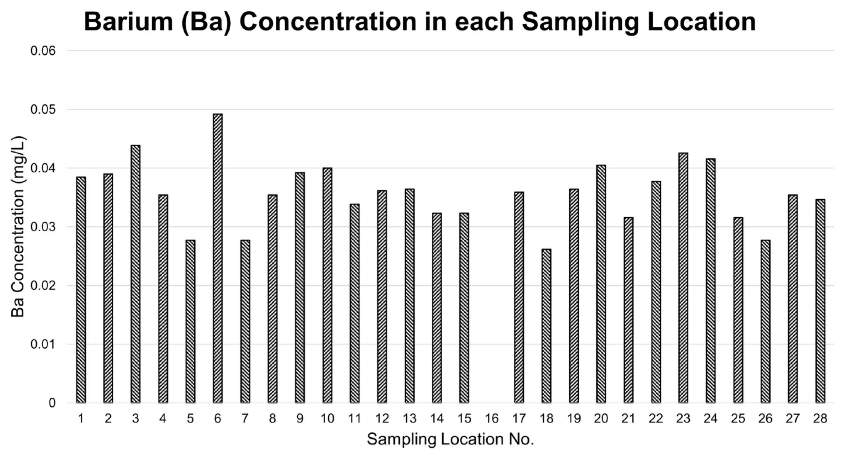
3.2.1. Barium
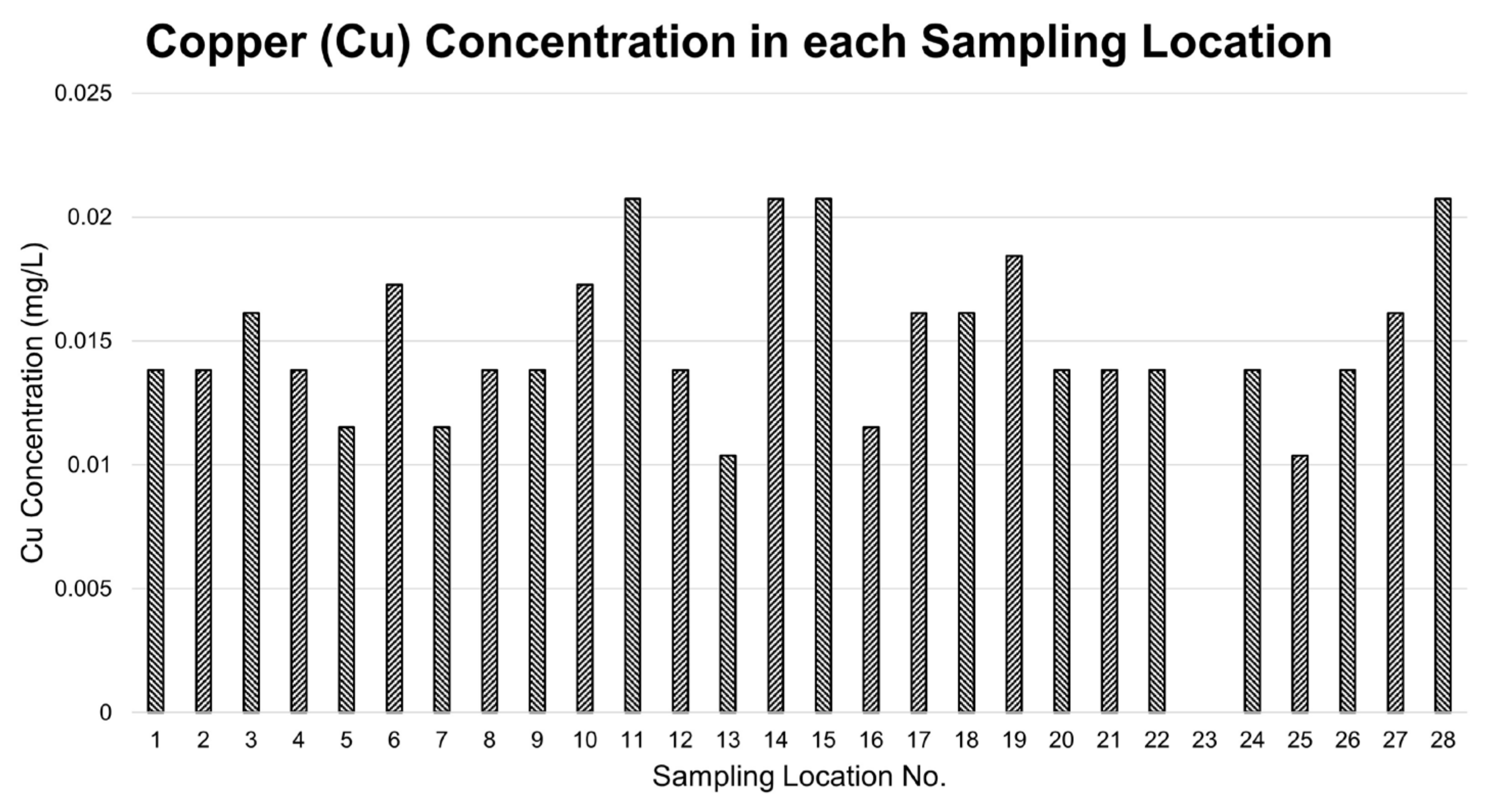
3.2.2. Copper
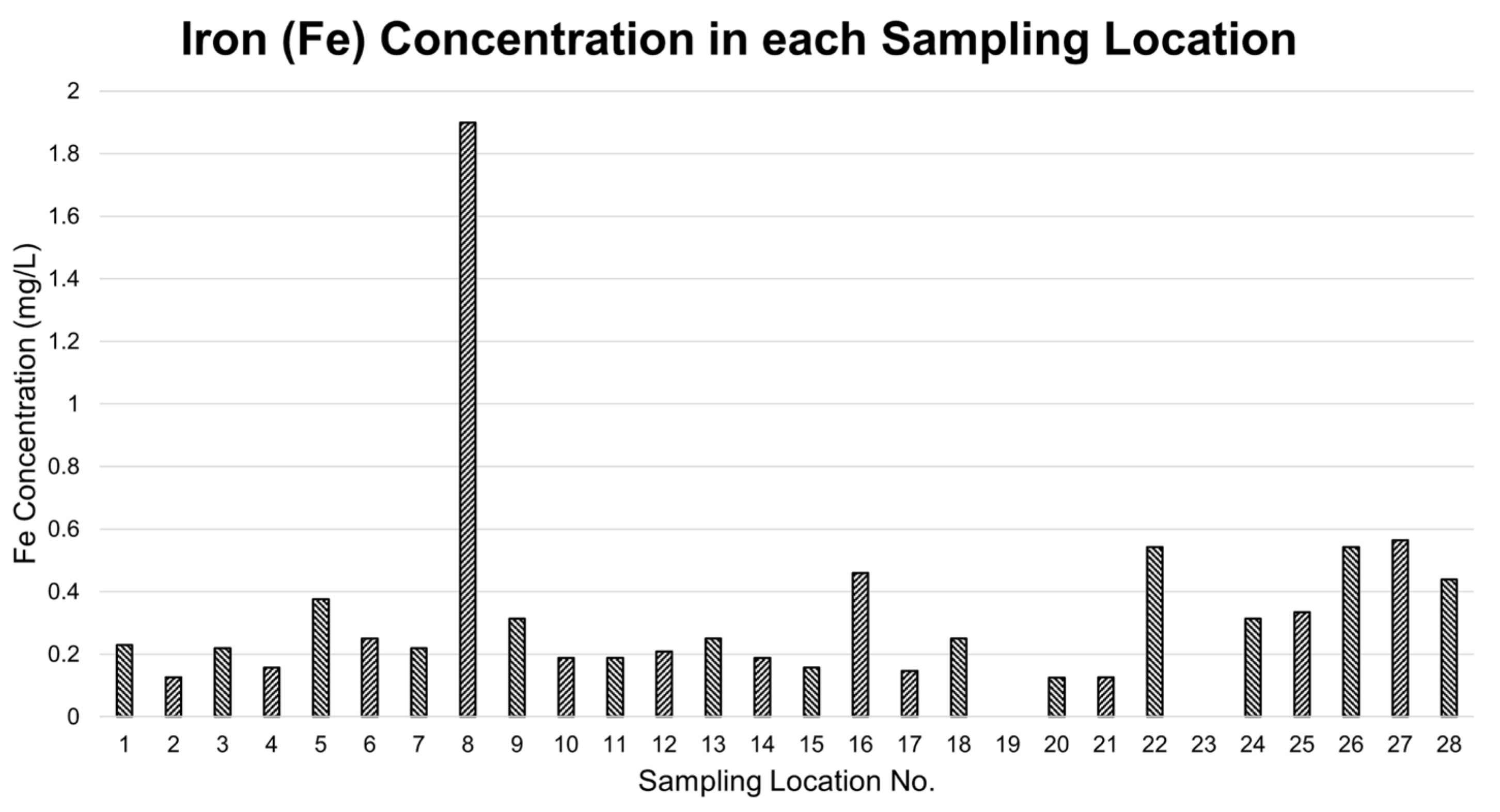
3.2.3. Iron
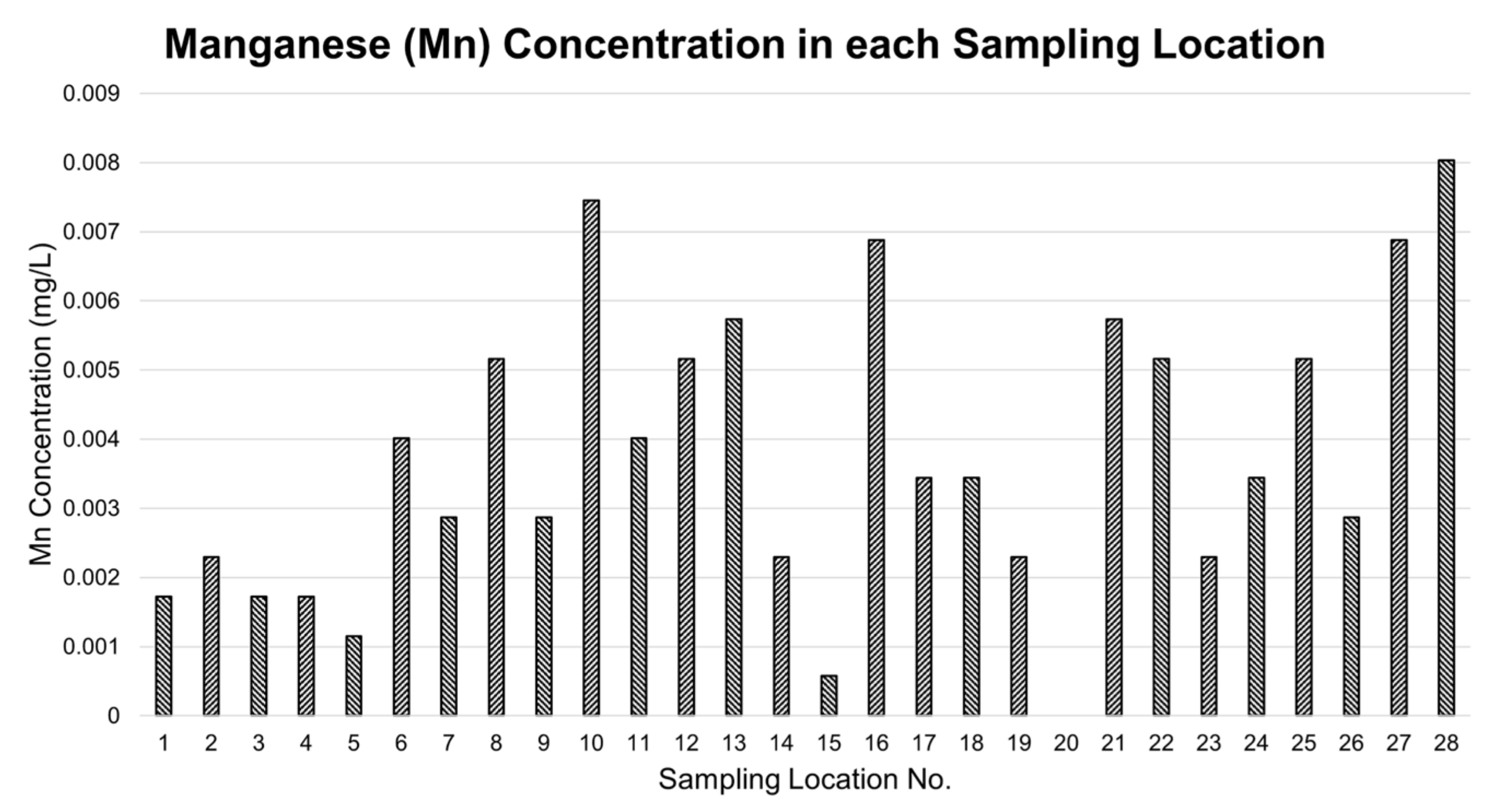
3.2.4. Manganese
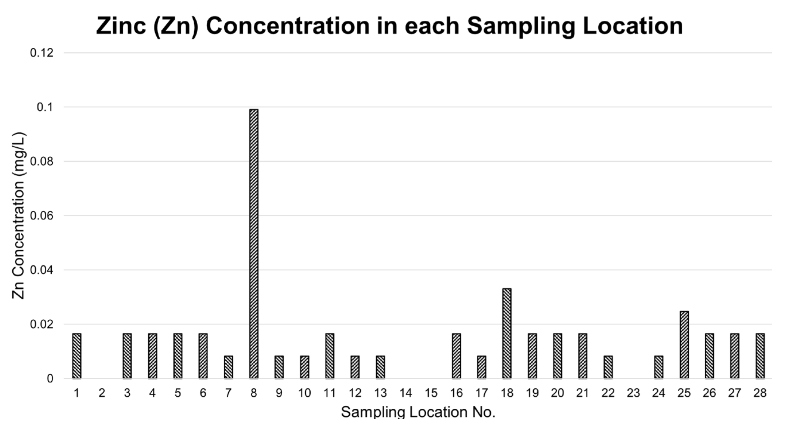
3.2.5. Zinc
3.3. Correlation Analysis
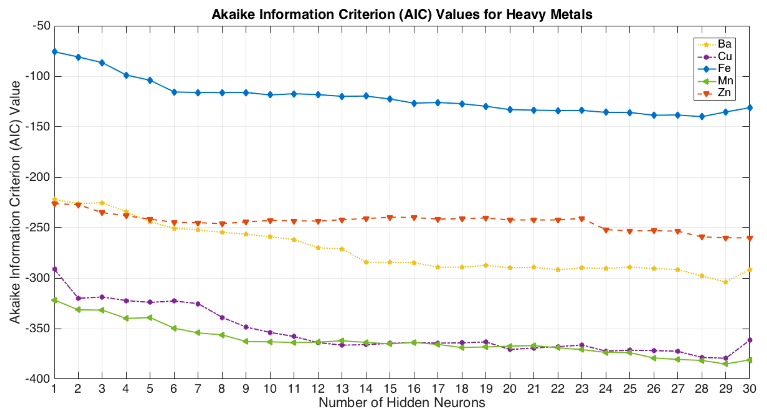
3.4. Spatial Concentration Mapping Using NN-PSO + EBK
3.5. Cross Validation and Spot Sampling Evaluation Results
4. Discussion
5. Conclusions
Author Contributions
Funding
Institutional Review Board Statement
Informed Consent Statement
Data Availability Statement
Acknowledgments
Conflicts of Interest
Appendix A

| Sampling No. | Barangay | Latitude | Longitude | Temp (°C) | pH | EC (µS/cm) | TDS (ppm) |
|---|---|---|---|---|---|---|---|
| 1 | Balingayan (Site 1) | 13.31903° N | 121.13432° E | 28.3 | 7.9 | 130 | 60 |
| 2 | Balingayan (Site 2) | 13.32454° N | 121.13555° E | 28.5 | 8.4 | 130 | 60 |
| 3 | Biga | 13.32791° N | 121.17312° E | 26.2 | 8.5 | 120 | 50 |
| 4 | Buhuan | 13.31451° N | 121.22395°E | 29.2 | 7.6 | 660 | 320 |
| 5 | Camansihan | 13.33399° N | 121.22656° E | 30.7 | 7.8 | 1200 | 590 |
| 6 | Canubing I | 13.35590° N | 121.14091° E | 27.1 | 8.8 | 130 | 50 |
| 7 | Comunal | 13.31267° N | 121.16494° E | 27.2 | 7.9 | 200 | 90 |
| 8 | Gutad | 13.35518° N | 121.25278° E | 32.4 | 7.1 | 900 | 440 |
| 9 | Ibaba East (Site 1) | 13.41517° N | 121.17836° E | 31.6 | 7.5 | 350 | 160 |
| 10 | Ibaba East (Site 2) | 13.41484° N | 121.17769° E | 32.5 | 7.5 | 970 | 480 |
| 11 | Ibaba West | 13.41478° N | 121.17676° E | 31.4 | 7.4 | 1820 | 900 |
| 12 | Ilaya | 13.41181° N | 121.18548° E | 31.1 | 7.1 | 780 | 380 |
| 13 | Lazareto | 13.42972° N | 121.19940° E | 31 | 7 | 990 | 490 |
| 14 | Maidlang | 13.39711° N | 121.22727° E | 32 | 7.5 | 600 | 290 |
| 15 | Managpi | 13.32512° N | 121.19595° E | 28.1 | 7.5 | 220 | 100 |
| 16 | Masipit | 13.38917° N | 121.16190° E | 31.5 | 7.3 | 570 | 270 |
| 17 | Nag-iba II | 13.34643° N | 121.25301° E | 30.6 | 7.3 | 820 | 400 |
| 18 | Pachoca | 13.41061° N | 121.16840° E | 29.2 | 8.1 | 690 | 340 |
| 19 | Palhi | 13.37502° N | 121.20703° E | 30.2 | 7.4 | 410 | 200 |
| 20 | Panggalaan | 13.30148° N | 121.19908° E | 30.1 | 7.6 | 140 | 160 |
| 21 | Panggalaan | 13.30027° N | 121.20041° E | 28.4 | 8.3 | 180 | 150 |
| 22 | Parang | 13.40059° N | 121.21769° E | 33.6 | 7.7 | 910 | 450 |
| 23 | Personas (Site 1) | 13.30623° N | 121.14083° E | 28.7 | 8.3 | 140 | 60 |
| 24 | Personas (Site 2) | 13.30930° N | 121.13945° E | 27.4 | 8.4 | 140 | 60 |
| 25 | San Vicente East | 13.31045° N | 121.17980° E | 32.9 | 7.6 | 750 | 370 |
| 26 | Sta. Cruz | 13.31633° N | 121.23461° E | 29.7 | 7.3 | 500 | 240 |
| 27 | Sta. Rita | 13.35212° N | 121.13091° E | 29.7 | 7.7 | 100 | 40 |
| 28 | Sto. Nino | 13.40712° N | 121.18545° E | 30.3 | 6.7 | 1140 | 560 |
Appendix B


Appendix C
| Brgy. No. | Barangay | Latitude | Longitude | Elev. (m) | Average MSE | ||||
|---|---|---|---|---|---|---|---|---|---|
| Ba | Cu | Fe | Mn | Zn | |||||
| 1 | Balingayan | 13.3241° N | 121.1407° E | 13.2 | 0.0000151 | 0.0000412 | 0.0000104 | 0.0000007 | 0.0000138 |
| 2 | Balite | 13.4131° N | 121.1580° E | 7.6 | 0.0002007 | 0.0002381 | 0.0009690 | 0.0000110 | 0.0025765 |
| 3 | Batino | 13.3494° N | 121.2201° E | 7.8 | 0.0000578 | 0.0000624 | 0.0009873 | 0.0000028 | 0.0003248 |
| 4 | Bayanan I | 13.3679° N | 121.1685° E | 8.8 | 0.0005507 | 0.0000240 | 0.0001122 | 0.0000040 | 0.0002384 |
| 5 | Bayanan II | 13.3560° N | 121.1699° E | 12.5 | 0.0002042 | 0.0001388 | 0.0005354 | 0.0000042 | 0.0001622 |
| 6 | Biga | 13.3270° N | 121.1733° E | 14.1 | 0.0000080 | 0.0000108 | 0.0000396 | 0.0000006 | 0.0001686 |
| 7 | Bondoc | 13.3867° N | 121.2010° E | 165.5 | 0.0000844 | 0.0000133 | 0.0025490 | 0.0000110 | 0.0003627 |
| 8 | Bucayao | 13.3066° N | 121.1915° E | 17.3 | 0.0000146 | 0.0000316 | 0.0000047 | 0.0000039 | 0.0000776 |
| 9 | Buhuan | 13.3106° N | 121.1915° E | 12.8 | 0.0000069 | 0.0000081 | 0.0002698 | 0.0000003 | 0.0000034 |
| 10 | Bulusan | 13.4037° N | 121.2012° E | 28.4 | 0.0000127 | 0.0000730 | 0.0009766 | 0.0000010 | 0.0000702 |
| 11 | Calero | 13.4159° N | 121.1831° E | 9.4 | 0.0000079 | 0.0001424 | 0.0000126 | 0.0000020 | 0.0000081 |
| 12 | Camansihan | 13.3428° N | 121.2290° E | 7.1 | 0.0000042 | 0.0000183 | 0.0004483 | 0.0000007 | 0.0004709 |
| 13 | Camilmil | 13.4061° N | 121.1760° E | 8.4 | 0.0000827 | 0.0000129 | 0.0000828 | 0.0000059 | 0.0000046 |
| 14 | Canubing I | 13.3554° N | 121.1423° E | 8.6 | 0.0000088 | 0.0000043 | 0.0030914 | 0.0000055 | 0.0012961 |
| 15 | Canubing II | 13.3261° N | 121.1216° E | 12.9 | 0.0002042 | 0.0001033 | 0.0002191 | 0.0000018 | 0.0017159 |
| 16 | Comunal | 13.3075° N | 121.1606° E | 19.5 | 0.0000085 | 0.0000694 | 0.0000558 | 0.0000008 | 0.0000270 |
| 17 | Guinobatan | 13.3829° N | 121.1818° E | 9.7 | 0.0003723 | 0.0000199 | 0.0003131 | 0.0000073 | 0.0000374 |
| 18 | Gulod | 13.3433° N | 121.2073° E | 9.0 | 0.0004521 | 0.0000160 | 0.0007486 | 0.0000049 | 0.0002808 |
| 19 | Gutad | 13.3597° N | 121.2464° E | 7.2 | 0.0001561 | 0.0000687 | 0.0075550 | 0.0000108 | 0.0021064 |
| 20 | Ibaba East | 13.4149° N | 121.1788° E | 6.6 | 0.0000009 | 0.0000016 | 0.0000250 | 0.0000008 | 0.0000022 |
| 21 | Ibaba West | 13.4146° N | 121.1762° E | 5.9 | 0.0000027 | 0.0000018 | 0.0000010 | 0.0000001 | 0.0000021 |
| 22 | Ilaya | 13.4129° N | 121.1840° E | 8.7 | 0.0000040 | 0.0000232 | 0.0000372 | 0.0000002 | 0.0000020 |
| 23 | Lalud | 13.3993° N | 121.1739° E | 9.1 | 0.0003669 | 0.0000186 | 0.0002229 | 0.0000068 | 0.0000209 |
| 24 | Lazareto | 13.4286° N | 121.1995° E | 12.9 | 0.0000251 | 0.0000371 | 0.0000305 | 0.0000012 | 0.0000589 |
| 25 | Libis | 13.4149° N | 121.1847° E | 9.2 | 0.0000074 | 0.0001006 | 0.0000018 | 0.0000010 | 0.0000036 |
| 26 | Lumang Bayan | 13.4009° N | 121.1816° E | 6.8 | 0.0001156 | 0.0000113 | 0.0001495 | 0.0000042 | 0.0000077 |
| 27 | Mahal na Pangalan | 13.4082° N | 121.1502° E | 9.0 | 0.0004217 | 0.0002451 | 0.0057978 | 0.0000094 | 0.0056021 |
| 28 | Maidlang | 13.3883° N | 121.2339° E | 8.3 | 0.0000427 | 0.0000111 | 0.0017492 | 0.0000014 | 0.0000401 |
| 29 | Malad | 13.3396° N | 121.1588° E | 10.8 | 0.0001085 | 0.0000189 | 0.0002558 | 0.0000093 | 0.0001421 |
| 30 | Malamig | 13.3439° N | 121.1456° E | 10.7 | 0.0000640 | 0.0000077 | 0.0002769 | 0.0000110 | 0.0001567 |
| 31 | Managpi | 13.3282° N | 121.1997° E | 18.0 | 0.0000321 | 0.0000051 | 0.0000465 | 0.0000014 | 0.0000330 |
| 32 | Masipit | 13.3869° N | 121.1603° E | 6.6 | 0.0000484 | 0.0000162 | 0.0001101 | 0.0000002 | 0.0000723 |
| 33 | Nag-Iba I | 13.3400° N | 121.2721° E | 8.5 | 0.0000893 | 0.0000313 | 0.0032634 | 0.0000108 | 0.0010670 |
| 34 | Nag-Iba II | 13.3470° N | 121.2622° E | 11.0 | 0.0000154 | 0.0000190 | 0.0016347 | 0.0000060 | 0.0006289 |
| 35 | Navotas | 13.3739° N | 121.2486° E | 7.5 | 0.0004349 | 0.0000114 | 0.0065142 | 0.0000019 | 0.0018669 |
| 36 | Pachoca | 13.4108° N | 121.1677° E | 6.0 | 0.0000441 | 0.0000266 | 0.0000465 | 0.0000024 | 0.0001095 |
| 37 | Palhi | 13.3750° N | 121.2070° E | 18.6 | 0.0001992 | 0.0000633 | 0.0003630 | 0.0000046 | 0.0000934 |
| 38 | Panggalaan | 13.3012° N | 121.1990° E | 17.9 | 0.0000164 | 0.0000234 | 0.0000402 | 0.0000039 | 0.0000126 |
| 39 | Parang | 13.4035° N | 121.2182° E | 9.5 | 0.0000148 | 0.0000209 | 0.0001279 | 0.0000015 | 0.0000127 |
| 40 | Patas | 13.3452° N | 121.1222° E | 12.9 | 0.0009213 | 0.0001269 | 0.0005874 | 0.0000021 | 0.0000333 |
| 41 | Personas | 13.3083° N | 121.1438° E | 14.5 | 0.0000006 | 0.0000300 | 0.0000213 | 0.0000001 | 0.0000028 |
| 42 | Puting Tubig | 13.3470° N | 121.1887° E | 7.3 | 0.0003178 | 0.0000788 | 0.0003261 | 0.0000037 | 0.0001840 |
| 43 | San Antonio | 13.4259° N | 121.1956° E | 14.0 | 0.0000013 | 0.0001353 | 0.0000519 | 0.0000045 | 0.0000587 |
| 44 | San Rafael | 13.4216° N | 121.1911° E | 6.4 | 0.0000099 | 0.0002183 | 0.0000171 | 0.0000053 | 0.0000280 |
| 45 | San Vicente Central | 13.4120° N | 121.1787° E | 8.6 | 0.0000010 | 0.0000086 | 0.0000024 | 0.0000011 | 0.0000011 |
| 46 | San Vicente East | 13.4098° N | 121.1798° E | 9.3 | 0.0000009 | 0.0000106 | 0.0000044 | 0.0000014 | 0.0000004 |
| 47 | San Vicente North | 13.4138° N | 121.1785° E | 6.7 | 0.0000003 | 0.0000045 | 0.0000005 | 0.0000003 | 0.0000001 |
| 48 | San Vicente South | 13.4095° N | 121.1779° E | 7.6 | 0.0000072 | 0.0000115 | 0.0000123 | 0.0000031 | 0.0000018 |
| 49 | San Vicente West | 13.4124° N | 121.1765° E | 7.8 | 0.0000005 | 0.0000040 | 0.0000024 | 0.0000005 | 0.0000010 |
| 50 | Santa Cruz | 13.3169° N | 121.2370° E | 12.1 | 0.0001231 | 0.0000173 | 0.0006697 | 0.0000002 | 0.0001946 |
| 51 | Santa Isabel | 13.3654° N | 121.1577° E | 5.3 | 0.0003942 | 0.0000233 | 0.0005533 | 0.0000043 | 0.0000575 |
| 52 | Santa Maria Village | 13.4093° N | 121.1748° E | 6.3 | 0.0000154 | 0.0000115 | 0.0000167 | 0.0000040 | 0.0000019 |
| 53 | Santa Rita | 13.3489° N | 121.1303° E | 11.1 | 0.0000139 | 0.0000317 | 0.0000140 | 0.0000002 | 0.0000081 |
| 54 | Santo Niño | 13.4066° N | 121.1848° E | 8.2 | 0.0000004 | 0.0000075 | 0.0000057 | 0.0000004 | 0.0000003 |
| 55 | Sapul | 13.3651° N | 121.1885° E | 14.3 | 0.0008450 | 0.0000108 | 0.0003983 | 0.0000126 | 0.0001391 |
| 56 | Silonay | 13.3992° N | 121.2248° E | 8.8 | 0.0000004 | 0.0000004 | 0.0000011 | 0.0000000 | 0.0000007 |
| 57 | Suqui | 13.4177° N | 121.2040° E | 11.1 | 0.0000057 | 0.0000434 | 0.0001749 | 0.0000019 | 0.0000464 |
| 58 | Tawagan | 13.3712° N | 121.1448° E | 8.6 | 0.0000693 | 0.0000169 | 0.0019052 | 0.0000004 | 0.0012349 |
| 59 | Tawiran | 13.3950° N | 121.1680° E | 7.0 | 0.0002160 | 0.0000253 | 0.0002604 | 0.0000030 | 0.0001365 |
| 60 | Tibag | 13.4123° N | 121.1730° E | 8.2 | 0.0000018 | 0.0000040 | 0.0000027 | 0.0000006 | 0.0000014 |
| 61 | Wawa | 13.4025° N | 121.1453° E | 8.8 | 0.0004609 | 0.0002441 | 0.0085841 | 0.0000055 | 0.0063922 |
References
- Pineda-Pineda, J.J.; Martínez-Martínez, C.T.; Méndez-Bermúdez, J.A.; Muñoz-Rojas, J.; Sigarreta, J.M. Application of Bipartite Networks to the Study of Water Quality. Sustainability 2020, 12, 5143. [Google Scholar] [CrossRef]
- Mekonnen, M.M.; Hoekstra, A.Y. Four billion people facing severe water scarcity. Sci. Adv. 2016, 2, e1500323. [Google Scholar] [CrossRef] [Green Version]
- Jha, M.K.; Shekhar, A.; Jenifer, M.A. Assessing groundwater quality for drinking water supply using hybrid fuzzy-GIS-based water quality index. Water Res. 2020, 179, 115867. [Google Scholar] [CrossRef] [PubMed]
- Department of Environment and Natural Resources—Mines and Geosciences Bureau. Geohazard Maps. Available online: http://www.region4b.mgb.gov.ph/28-geohazard-maps/98-geohazard-maps (accessed on 25 October 2021).
- Philippine Statistics Authority. Compendium of Philippine Environment Statistics Component 2: Environmental Resources and their Use. Available online: https://psa.gov.ph/press-releases/id/163678 (accessed on 25 October 2021).
- Kumar, A.; Cabral-Pinto, M.; Kumar, A.; Kumar, M.; Dinis, P.A. Estimation of Risk to the Eco-Environment and Human Health of Using Heavy Metals in the Uttarakhand Himalaya, India. Appl. Sci. 2020, 10, 7078. [Google Scholar] [CrossRef]
- Kumar, A.; Jigyasu, D.K.; Kumar, A.; Subrahmanyam, G.; Mondal, R.; Shabnam, A.A.; Cabral-Pinto, M.M.S.; Malyan, S.K.; Chaturvedi, A.K.; Gupta, D.K.; et al. Nickel in terrestrial biota: Comprehensive review on contamination, toxicity, tolerance and its remediation approaches. Chemosphere 2021, 275, 129996. [Google Scholar] [CrossRef] [PubMed]
- Kumar, A.; Cabral Pinto, M.; Candeias, C.; Dinis, P.A. Baseline maps of potentially toxic elements in the soil of Garhwal Himalayas, India: Assessment of their eco-environmental and human health risks. Land Degrad. Dev. 2021, 10, 3984. [Google Scholar] [CrossRef]
- Hartzler, D.A.; Jain, J.C.; McIntyre, D.L. Development of a subsurface LIBS sensor for in situ groundwater quality monitoring with applications in CO 2 leak sensing in carbon sequestration. Sci. Rep. 2019, 9, 1–10. [Google Scholar]
- Bu, X.; Koide, K.; Carder, E.J.; Welch, C.J. Rapid analysis of residual palladium in pharmaceutical development using a catalysis-based fluorometric method. Org. Process Res. Dev. 2013, 17, 108–113. [Google Scholar] [CrossRef]
- Farghaly, O.A.; Hameed, R.A.; Abu-Nawwas, A.A.H. Analytical application using modern electrochemical techniques. Int. J. Electrochem. Sci. 2014, 9, 3287–3318. [Google Scholar]
- Kudr, J.; Richtera, L.; Nejdl, L.; Xhaxhiu, K.; Vitek, P.; Rutkay-Nedecky, B.; Hynek, D.; Kopel, P.; Adam, V.; Kizek, R. Improved electrochemical detection of zinc ions using electrode modified with electrochemically reduced graphene oxide. Materials 2016, 9, 31. [Google Scholar] [CrossRef]
- Estela, J.M.; Tomás, C.; Cladera, A.; Cerda, V. Potentiometric stripping analysis: A review. Crit. Rev. Anal. Chem. 1995, 25, 91–141. [Google Scholar] [CrossRef]
- Khadro, B.; Sikora, A.; Loir, A.S.; Errachid, A.; Garrelie, F.; Donnet, C.; Jaffrezic-Renault, N. Electrochemical performances of B doped and undoped diamond-like carbon (DLC) films deposited by femtosecond pulsed laser ablation for heavy metal detection using square wave anodic stripping voltammetric (SWASV) technique. Sens. Actuators B Chem. 2011, 155, 120–125. [Google Scholar] [CrossRef]
- Avuthu, S.G.R.; Narakathu, B.B.; Eshkeiti, A.; Emamian, S.; Bazuin, B.J.; Joyce, M.; Atashbar, M.Z. Detection of heavy metals using fully printed three electrode electrochemical sensor. In SENSORS; IEEE: New York, NY, USA, 2014; pp. 669–672. [Google Scholar]
- Cheng, L.; Liu, X.; Lei, J.; Ju, H. Low-potential electrochemiluminescent sensing based on surface unpassivation of CdTe quantum dots and competition of analyte cation to stabilizer. Anal. Chem. 2010, 82, 3359–3364. [Google Scholar] [CrossRef] [PubMed]
- Bansod, B.; Kumar, T.; Thakur, R.; Rana, S.; Singh, I. A review on various electrochemical techniques for heavy metal ions detection with different sensing platforms. Biosens. Bioelectron. 2017, 94, 443–455. [Google Scholar] [CrossRef]
- Borgese, L.; Zacco, A.; Bontempi, E.; Pellegatta, M.; Vigna, L.; Patrini, L.; Riboldi, L.; Rubino, F.M.; Depero, L.E. Use of total reflection X-ray fluorescence (TXRF) for the evaluation of heavy metal poisoning due to the improper use of a traditional ayurvedic drug. J. Pharm. Biomed. Anal. 2010, 52, 787–790. [Google Scholar] [CrossRef]
- De Jesus, K.; Senoro, D.B.; Dela Cruz, J.C.; Chan, E.B. A Hybrid Neural Network—Particle Swarm Optimization In-formed Spatial Interpolation Technique for Groundwater Quality Mapping in a Small Island Province of the Philippines. Toxics 2021, 9, 273. [Google Scholar] [CrossRef] [PubMed]
- El-Rawy, M.; Fathi, H.; Abdalla, F. Integration of remote sensing data and in situ measurements to monitor the water quality of the Ismailia Canal, Nile Delta, Egypt. Environ. Geochem. Health 2020, 42, 2101–2120. [Google Scholar] [CrossRef] [PubMed]
- Solis, K.L.B.; Macasieb, R.Q.; Parangat, R.C.; Resurreccion, A.C.; Ocon, J.D. Spatiotemporal Variation of Groundwater Arsenic in Pampanga, Philippines. Water 2020, 12, 2366. [Google Scholar] [CrossRef]
- Tiankao, W.; Chotpantarat, S. Risk assessment of arsenic from contaminated soils to shallow groundwater in Ong Phra Sub-District, Suphan Buri Province, Thailand. J. Hydrol. Reg. Stud. 2018, 19, 80–96. [Google Scholar] [CrossRef]
- Mogaji, K.A. Application of vulnerability modeling techniques in groundwater resources management: A comparative study. Appl. Water Sci. 2018, 8, 1–24. [Google Scholar] [CrossRef] [Green Version]
- Nistor, M.M.; Rahardjo, H.; Satyanaga, A.; Hao, K.Z.; Xiaosheng, Q.; Sham, A.W.L. Investigation of groundwater table distribution using borehole piezometer data interpolation: Case study of Singapore. Eng. Geol. 2020, 271, 105590. [Google Scholar] [CrossRef]
- Rusydi, A.F.; Onodera, S.I.; Saito, M.; Ioka, S.; Maria, R.; Ridwansyah, I.; Delinom, R.M. Vulnerability of groundwater to iron and manganese contamination in the coastal alluvial plain of a developing Indonesian city. SN Appl. Sci. 2021, 3, 1–12. [Google Scholar] [CrossRef]
- Lado, L.R.; Polya, D.; Winkel, L.; Berg, M.; Hegan, A. Modelling arsenic hazard in Cambodia: A geostatistical approach using ancillary data. Appl. Geochem. 2008, 23, 3010–3018. [Google Scholar] [CrossRef]
- Viossanges, M.; Pavelic, P.; Rebelo, L.M.; Lacombe, G.; Sotoukee, T. Regional mapping of groundwater resources in data-scarce regions: The case of Laos. Hydrology 2018, 5, 2. [Google Scholar] [CrossRef] [Green Version]
- Giang, P.Q.; Nakhapakorn, K.; Ussawarujikulchai, A. Effectiveness of different spatial interpolators in estimating heavy metal contamination in shallow groundwater: A case study of arsenic contamination in Hanoi, Vietnam. Environ. Nat. Resour. J. 2011, 9, 31–37. [Google Scholar]
- Agutaya, C.A.C.; Zamora, J.T. Developmental Projects in Calapan City, Philippines: Localization Perspectives. Am. J. Educ. Res. 2018, 6, 133–136. [Google Scholar]
- United States Environmental Protection Agency (U.S. E.P.A). Operating Procedure for In Situ Water Quality Monitoring (SESDPROC-111-R4). Available online: https://www.epa.gov/sites/default/files/2015-06/documents/Insitu-Water-Quality-Mon.pdf (accessed on 16 December 2021).
- Hanna Instruments. HI9811-5 Portable pH/EC/TDS/Temperature. Available online: https://www.hannainst.com/portable-ph-ec-tds-temperature-meter-hi9811-5.html (accessed on 16 December 2021).
- Magalona, M.L.; Peralta, M.M.; Lacsamana, M.S.; Sabularse, V.C.; Pelegrina, A.B.; De Guzman, C.C. Analysis of Inorganic Arsenic (As (III) and Total As) and Some Physicochemical Parameters in Groundwater Samples from Selected Areas in Bulacan, Batangas, and Laguna, Philippines. KIMIKA 2019, 30, 28–38. [Google Scholar] [CrossRef]
- Groover, K.D.; Izbicki, J.A. Elemental analysis using a handheld X-ray fluorescence spectrometer (No. 2016-3043). U.S. Geol. Surv. Fact Sheet 2016, 2015–3043. [Google Scholar] [CrossRef]
- Analytical Methods Committee AMCTB No. 89. Hand-held X-ray fluorescence spectrometry. Anal. Methods 2019, 11, 2498–2501. [Google Scholar] [CrossRef]
- Muramatsu, Y.; Izawa, R.; Nishioka, H.; Nogami, T. X-ray fluorescence analysis of dilute heavy-metals in water using a portable x-ray fluorescence spectrometer with the metal-adsorbent, tobermorite. X-sen Bunseki No Shinpo 2009, 40, 195–201. [Google Scholar]
- Pearson, D.; Weindorf, D.C.; Chakraborty, S.; Li, B.; Koch, J.; Van Deventer, P.; de Wet, J.; Kusi, N.Y. Analysis of metal-laden water via portable X-ray fluorescence spectrometry. J. Hydrol. 2018, 561, 267–276. [Google Scholar] [CrossRef]
- Zhou, S.; Yuan, Z.; Cheng, Q.; Zhang, Z.; Yang, J. Rapid in situ determination of heavy metal concentrations in polluted water via portable XRF: Using Cu and Pb as example. Environ. Pollut. 2018, 243, 1325–1333. [Google Scholar] [CrossRef]
- Pearson, D.; Chakraborty, S.; Duda, B.; Li, B.; Weindorf, D.C.; Deb, S.; Brevik, E.; Ray, D.P. Water analysis via portable X-ray fluorescence spectrometry. J. Hydrol. 2017, 544, 172–179. [Google Scholar] [CrossRef] [Green Version]
- Crocombe, R.A.; Leary, P.E.; Kammrath, B.W. Portable Spectroscopy and Spectrometry, Applications; John Wiley & Sons: Hoboken, NJ, USA, 2021; Volume 2, ISBN 978-111-963-640-3. [Google Scholar]
- Magesh, N.S.; Chandrasekar, N.; Elango, L. Occurrence and distribution of fluoride in the groundwater of the Tamiraparani River basin, South India: A geostatistical modeling approach. Environ. Earth Sci. 2016, 75, 1–16. [Google Scholar] [CrossRef]
- Shariati, M.; Mafipour, M.S.; Mehrabi, P.; Bahadori, A.; Zandi, Y.; Salih, M.N.; Nguyen, H.; Dou, J.; Song, X.; Poi-Ngian, S. Application of a hybrid artificial neural network-particle swarm optimization (ANN-PSO) model in behavior prediction of channel shear connectors embedded in normal and high-strength concrete. Appl. Sci. 2019, 9, 5534. [Google Scholar] [CrossRef] [Green Version]
- Kayabasi, E.; Ozturk, S.; Celik, E.; Kurt, H. Determination of cutting parameters for silicon wafer with a Diamond Wire Saw using an artificial neural network. Sol. Energy 2017, 149, 285–293. [Google Scholar] [CrossRef]
- Ozturk, S.; Kayabasi, E.; Celik, E.; Kurt, H. Determination of lapping parameters for silicon wafer using an artificial neural network. J. Mater. Sci.: Mater. Electron. 2018, 29, 260–270. [Google Scholar] [CrossRef]
- Lin, Y.H.; Hu, Y.C. Electrical energy management based on a hybrid artificial neural network-particle swarm optimization-integrated two-stage non-intrusive load monitoring process in smart homes. Processes 2018, 6, 236. [Google Scholar] [CrossRef] [Green Version]
- World Health Organization. Guidelines for Drinking-Water Quality, 3rd ed.; World Health Organization: Geneva, Switzerland, 2004; Volume 1, ISBN 92-4-154638-7. [Google Scholar]
- Department of Health—Food and Drug Administration. Administrative Order No. 2017-0010—Philippine National Standards for Drinking Water of 2017. Available online: https://www.fda.gov.ph/administrative-order-no-2017-0010-philippine-national-standards-for-drinking-water-of-2017 (accessed on 25 October 2021).
- Li, H.; Shi, A.; Li, M.; Zhang, X. Effect of pH, temperature, dissolved oxygen, and flow rate of overlying water on heavy metals release from storm sewer sediments. J. Chem. 2013, 2013, 434012. [Google Scholar] [CrossRef]
- Zhu, K.; Blum, P.; Ferguson, G.; Balke, K.D.; Bayer, P. The geothermal potential of urban heat islands. Environ. Res. Lett. 2010, 5, 044002. [Google Scholar] [CrossRef]
- Lomboy, M.; Riego de Dios, J.; Magtibay, B.; Quizon, R.; Molina, V.; Fadrilan-Camacho, V.; See, J.; Enoveso, A.; Barbosa, L.; Agravante, A. Updating national standards for drinking-water: A Philippine experience. J. Water Health 2017, 15, 288–295. [Google Scholar] [CrossRef] [PubMed]
- Edwards, K.A.; Classen, G.A.; Schroten, E.H.J. The Water Resource in Tropical Africa and Its Exploitation. Available online: https://www.ilri.org/publications/water-resource-tropical-africa-and-its-exploitation (accessed on 20 November 2021).
- Anyanwu, B.O.; Ezejiofor, A.N.; Igweze, Z.N.; Orisakwe, O.E. Heavy metal mixture exposure and effects in developing nations: An update. Toxics 2018, 6, 65. [Google Scholar] [CrossRef] [Green Version]
- Fenton, T.R.; Huang, T. Systematic review of the association between dietary acid load, alkaline water and cancer. BMJ open 2016, 6, e010438. [Google Scholar] [CrossRef] [PubMed]
- Jan, A.T.; Azam, M.; Siddiqui, K.; Ali, A.; Choi, I.; Haq, Q.M. Heavy metals and human health: Mechanistic insight into toxicity and counter defense system of antioxidants. Int. J. Mol. Sci. 2015, 16, 29592–29630. [Google Scholar] [CrossRef] [Green Version]
- Patil, V.T.; Patil, P.R. Physicochemical Analysis of Selected Groundwater Samples of Amalner Town in Jalgaon District, Maharashtra, India. E-J. Chem. 2010, 7, 111–116. [Google Scholar] [CrossRef] [Green Version]
- Oyem, H.H.; Oyem, I.M.; Ezeweali, D. Temperature, pH, electrical conductivity, total dissolved solids and chemical oxygen demand of groundwater in Boji-BojiAgbor/Owa area and immediate suburbs. Res. J. Environ. Sci. 2014, 8, 444. [Google Scholar] [CrossRef] [Green Version]
- Ramasamy, S. Barium in Drinking Water—Background document for development of WHO Guidelines for Drinking-water Quality. Available online: https://www.who.int/water_sanitation_health/water-quality/guidelines/chemicals/barium-background-jan17.pdf (accessed on 26 October 2021).
- Kroschwitz, J.I.; Howe-Grant, M. Kirk-Othmer Encyclopedia of Chemical Technology, 3rd ed.; Grayson, M., Eckroth, D., Eds.; John Wiley and Sons: New York, NY, USA, 1978; Volume 3, pp. 457–463. [Google Scholar]
- Miner, S. Air Pollution Aspects of Barium and Its Compounds; Contract No. Ph-22-68-25; Litton Systems, Inc.: Bethesda, MD, USA, 1969; p. 69. [Google Scholar]
- Pinto, V.M.; Hartmann, L.A. Flow-by-flow chemical stratigraphy and evolution of thirteen Serra Geral Group basalt flows from Vista Alegre, southernmost Brazil. An. Acad. Bras. Cienc. 2011, 83, 425–440. [Google Scholar] [CrossRef] [Green Version]
- Vieira, I.F.B.; Rolim Neto, F.C.; Carvalho, M.N.; Caldas, A.M.; Costa, R.C.A.; Silva, K.S.D.; Parahyba, R.D.B.V.; Pacheco, F.A.L.; Fernendes, L.F.S.; Pissarra, T.C.T. Water Security Assessment of Groundwater Quality in an Anthropized Rural Area from the Atlantic Forest Biome in Brazil. Water 2020, 12, 623. [Google Scholar] [CrossRef] [Green Version]
- Beyene, G.; Aberra, D.; Fufa, F. Evaluation of the suitability of groundwater for drinking and irrigation purposes in Jimma Zone of Oromia, Ethiopia. Groundw. Sustain. Dev. 2019, 9, 100216. [Google Scholar] [CrossRef]
- Carasek, F.L.; Baldissera, R.; Oliveira, J.V.; Scheibe, L.F.; Dal Magro, J. Quality of the groundwater of the Serra Geral aquifer system of Santa Catarina west region, Brazil. Groundw. Sustain. Dev. 2020, 10, 100346. [Google Scholar] [CrossRef]
- Maher, K. The dependence of chemical weathering rates on fluid residence time. Earth Planet. Sci. Lett. 2010, 294, 101–110. [Google Scholar] [CrossRef]
- Sholehhudin, M.; Azizah, R.; Sham, A.S.S.M.; Amiruddin, Z. Analysis of Heavy Metals (Cadmium, Chromium, Lead, Manganese, and Zinc) in Well Water in East Java Province, Indonesia. Malays. J. Med. Health Sci. 2021, 17, 146–153. [Google Scholar]
- Zhang, Z.; Xiao, C.; Adeyeye, O.; Yang, W.; Liang, X. Source and mobilization mechanism of iron, manganese and arsenic in groundwater of Shuangliao City, Northeast China. Water 2020, 12, 534. [Google Scholar] [CrossRef] [Green Version]
- Abou Zakhem, B.; Al-Charideh, A.; Kattaa, B. Using principal component analysis in the investigation of groundwater hydrochemistry of Upper Jezireh Basin, Syria. Hydrol. Sci. J. 2017, 62, 2266–2279. [Google Scholar]
- Sunkari, E.D.; Abu, M. Hydrochemistry with special reference to fluoride contamination in groundwater of the Bongo District, Upper East Region, Ghana. Sustain. Water. Resour. Manag. 2019, 5, 1803–1814. [Google Scholar] [CrossRef]
- Wali, S.U.; Alias, N.; Harun, S.B. Reevaluating the hydrochemistry of groundwater in basement complex aquifers of Kaduna Basin, NW Nigeria using multivariate statistical analysis. Environ. Earth Sci. 2021, 80, 1–25. [Google Scholar] [CrossRef]
- Senoro, D.B.; De Jesus, K.L.M.; Yanuaria, C.A.; Bonifacio, P.B.; Manuel, M.T.; Wang, B.N.; Kao, C.C.; Wu, T.N.; Ney, F.P.; Natal, P. Rapid site assessment in a small island of the Philippines contaminated with mine tailings using ground and areal technique: The environmental quality after twenty years. In IOP Conference Series: Earth and Environmental Science; IOP Publishing: Bristol, UK, 2019; Volume 351, p. 012022. [Google Scholar]
- Wright, N. Small Island Developing States, disaster risk management, disaster risk reduction, climate change adaptation and tourism. Background Paper for the Global Assessment Report on DRR 2013. 2013. Available online: https://www.preventionweb.net/english/hyogo/gar/2013/en/bgdocs/Wright,%20N.,%202013.pdf (accessed on 20 November 2021).
- Lopez-Maldonado, Y.; Batllori-Sampedro, E.; Binder, C.R.; Fath, B.D. Local groundwater balance model: Stakeholders’ efforts to address groundwater monitoring and literacy. Hydrol. Sci. J. 2017, 62, 2297–2312. [Google Scholar] [CrossRef]
- Galhardi, J.A.; Bonotto, D.M. Hydrogeochemical features of surface water and groundwater contaminated with acid mine drainage (AMD) in coal mining areas: A case study in southern Brazil. Environ. Sci. Pollut. 2016, 23, 18911–18927. [Google Scholar]
- Williams, M.; Todd, G.D.; Roney, N.; Crawford, J.; Coles, C.; McClure, P.R.; Garey, J.D.; Zaccaria, K.; Citra, M. Toxicological Profile for Manganese; Agency for Toxic Substances and Disease Registry (US): Atlanta, GA, USA, 2012. [Google Scholar]
- Erikson, K.M.; Thompson, K.; Aschner, J.; Aschner, M. Manganese neurotoxicity: A focus on the neonate. Pharmacol. Ther. 2007, 113, 369–377. [Google Scholar] [CrossRef] [Green Version]
- Bhasin, G.; Kauser, H.; Athar, M. Iron augments stage-I and stage-II tumor promotion in murine skin. Cancer Lett. 2002, 183, 113–122. [Google Scholar] [CrossRef]
- Grazuleviciene, R.; Nadisauskiene, R.; Buinauskiene, J.; Grazulevicius, T. Effects of elevated levels of manganese and iron in drinking water on birth outcomes. Pol. J. Environ. Stud. 2009, 18, 819–825. [Google Scholar]
- Kravchenko, J.; Darrah, T.H.; Miller, R.K.; Lyerly, H.K.; Vengosh, A. A review of the health impacts of barium from natural and anthropogenic exposure. Environ. Geochem. Health. 2014, 36, 797–814. [Google Scholar] [CrossRef] [PubMed]
- MacDonald, A.M.; Bonsor, H.C.; Ahmed, K.M.; Burgess, W.G.; Basharat, M.; Calow, R.C.; Dixit, A.; Foster, S.S.D.; Gopal, K.; Lapworth, D.J.; et al. Groundwater quality and depletion in the Indo-Gangetic Basin mapped from in situ observations. Nat. Geosci. 2016, 9, 762–766. [Google Scholar] [CrossRef]


| Sampling No. | Temperature (°C) | pH | EC (µS/cm) | TDS (ppm) |
|---|---|---|---|---|
| 1 | 28.3 | 7.9 | 130 | 60 |
| 2 | 28.5 | 8.4 | 130 | 60 |
| 3 | 26.2 | 8.5 | 120 | 50 |
| 4 | 29.2 | 7.6 | 660 | 320 |
| 5 | 30.7 | 7.8 | 1200 | 590 |
| 6 | 27.1 | 8.8 | 130 | 50 |
| 7 | 27.2 | 7.9 | 200 | 90 |
| 8 | 32.4 | 7.1 | 900 | 440 |
| 9 | 31.6 | 7.5 | 350 | 160 |
| 10 | 32.5 | 7.5 | 970 | 480 |
| 11 | 31.4 | 7.4 | 1820 | 900 |
| 12 | 31.1 | 7.1 | 780 | 380 |
| 13 | 31.0 | 7.0 | 990 | 490 |
| 14 | 32.0 | 7.5 | 600 | 290 |
| 15 | 28.1 | 7.5 | 220 | 100 |
| 16 | 31.5 | 7.3 | 570 | 270 |
| 17 | 30.6 | 7.3 | 820 | 400 |
| 18 | 29.2 | 8.1 | 690 | 340 |
| 19 | 30.2 | 7.4 | 410 | 200 |
| 20 | 30.1 | 7.6 | 140 | 160 |
| 21 | 28.4 | 8.3 | 180 | 150 |
| 22 | 33.6 | 7.7 | 910 | 450 |
| 23 | 28.7 | 8.3 | 140 | 60 |
| 24 | 27.4 | 8.4 | 140 | 60 |
| 25 | 32.9 | 7.6 | 750 | 370 |
| 26 | 29.7 | 7.3 | 500 | 240 |
| 27 | 29.7 | 7.7 | 100 | 40 |
| 28 | 30.3 | 6.7 | 1140 | 560 |
| WHO [45] | 30.0 | 6.5–8.5 | 400 | 1000 |
| PNSDW [46] | 6.5–8.5 | - | 600 |
| Parameter, mg/L | WHO | USEPA (2009) | PNSDW 2017 |
|---|---|---|---|
| Ba | 0.7 [56] | 2.00 | 0.70 |
| Cu | 1.30 [45] | 1.30 | 1.00 |
| Fe | - | 0.30 | 1.00 |
| Mn | 0.40 1 | 0.05 | 0.40 |
| Zn | - | 5.00 | - |
| Parameter | Temp | pH | EC | TDS |
|---|---|---|---|---|
| Temp | 1.000 | |||
| pH | −0.665 ** | 1.000 | ||
| EC | 0.657 ** | −0.602 ** | 1.000 | |
| TDS | 0.664 ** | −0.603 ** | 0.995 ** | 1.000 |
| Metal | Ba | Cu | Fe | Mn | Zn |
|---|---|---|---|---|---|
| Ba | 1 | ||||
| Cu | 0.055 | 1 | |||
| Fe | −0.136 | −0.001 | 1 | ||
| Mn | −0.235 | 0.072 | 0.320 | 1 | |
| Zn | −0.089 | 0.013 | 0.870 ** | 0.190 | 1 |
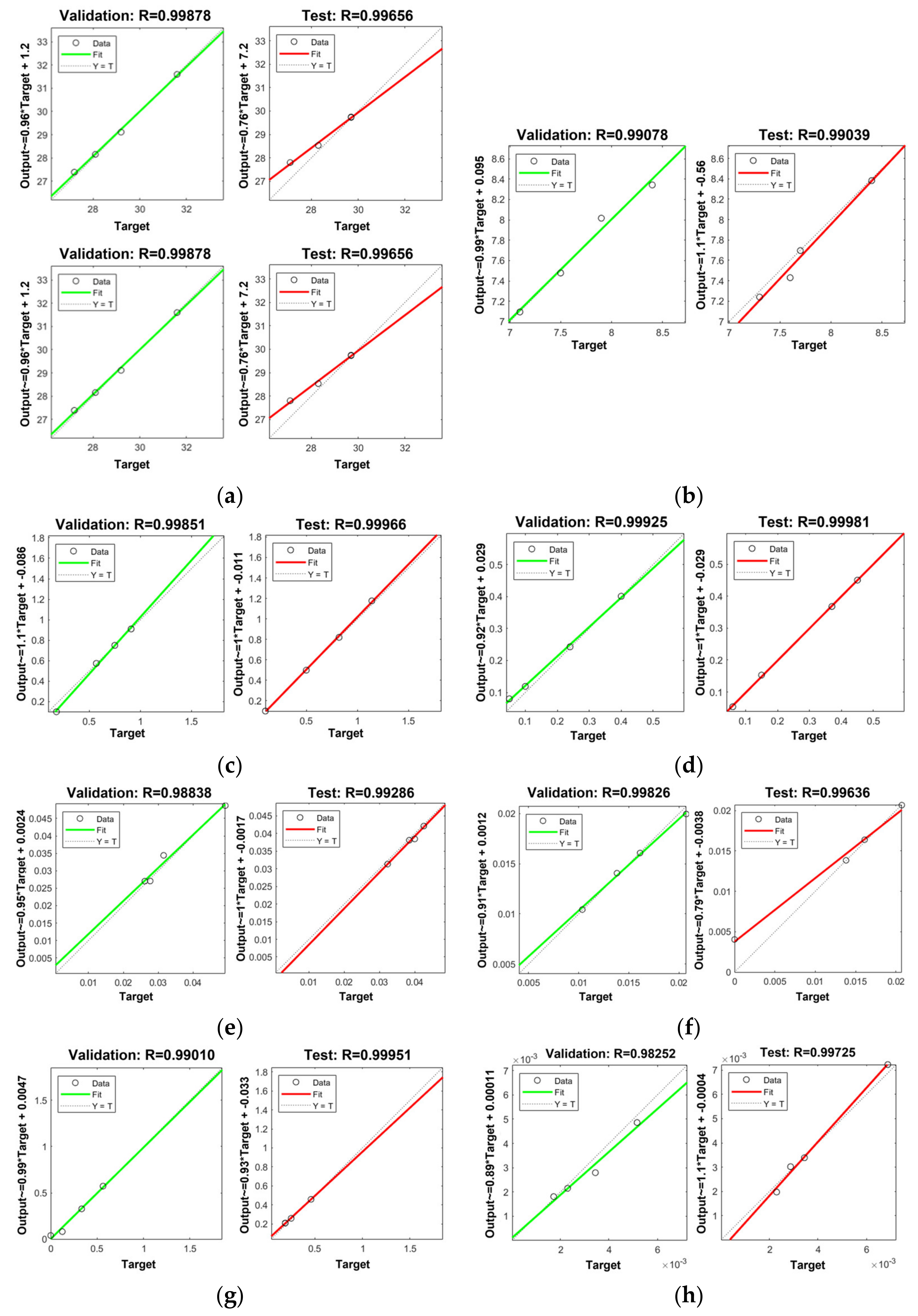
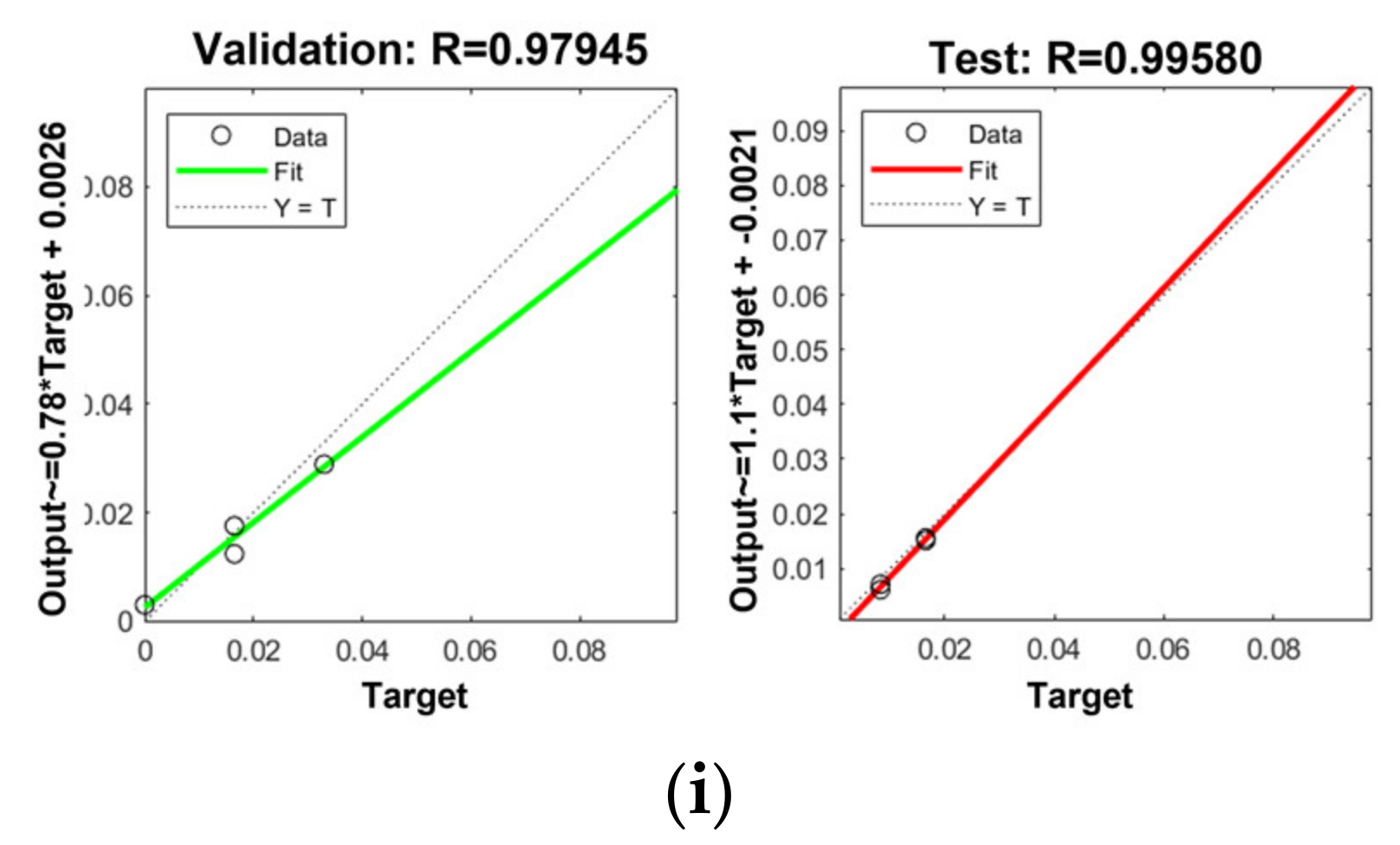
| Hidden Neurons | No. of Particles | No. of Iterations | Elapsed Time (sec) | MSE | R | ||
|---|---|---|---|---|---|---|---|
| Validation | Testing | ||||||
| Temp | 25 | 3 | 2000 | 180.38559 | 0.01204 | 0.99878 | 0.99656 |
| pH | 29 | 10 | 2000 | 119.16085 | 0.00434 | 0.99078 | 0.99039 |
| EC | 30 | 1 | 2000 | 163.34882 | 0.00155 | 0.99851 | 0.99966 |
| TDS | 27 | 3 | 2000 | 337.90592 | 0.00032 | 0.99925 | 0.99981 |
| Ba | 29 | 1 | 2000 | 172.62202 | 2.44 × 10⁻⁶ | 0.98838 | 0.99286 |
| Cu | 29 | 3 | 2000 | 366.12861 | 1.64 × 10⁻⁷ | 0.99826 | 0.99636 |
| Fe | 28 | 3 | 2000 | 139.78693 | 0.00091 | 0.99010 | 0.99951 |
| Mn | 29 | 5 | 2000 | 115.26285 | 1.34 × 10⁻⁷ | 0.98252 | 0.99725 |
| Zn | 30 | 1 | 2000 | 142.60618 | 1.08 × 10⁻⁵ | 0.97945 | 0.99580 |
| Criteria | Temp | pH | EC | TDS | Ba | Cu | Fe | Mn | Zn |
|---|---|---|---|---|---|---|---|---|---|
| R | 0.989 | 0.990 | 0.934 | 0.977 | 0.994 | 0.976 | 0.985 | 0.975 | 0.984 |
| Criteria | Ba | Cu | Fe | Mn | Zn |
|---|---|---|---|---|---|
| MSE | 0.0001404 | 0.0000542 | 0.0006260 | 0.0000037 | 0.0004141 |
Publisher’s Note: MDPI stays neutral with regard to jurisdictional claims in published maps and institutional affiliations. |
© 2021 by the authors. Licensee MDPI, Basel, Switzerland. This article is an open access article distributed under the terms and conditions of the Creative Commons Attribution (CC BY) license (https://creativecommons.org/licenses/by/4.0/).
Share and Cite
Senoro, D.B.; de Jesus, K.L.M.; Mendoza, L.C.; Apostol, E.M.D.; Escalona, K.S.; Chan, E.B. Groundwater Quality Monitoring Using In-Situ Measurements and Hybrid Machine Learning with Empirical Bayesian Kriging Interpolation Method. Appl. Sci. 2022, 12, 132. https://0-doi-org.brum.beds.ac.uk/10.3390/app12010132
Senoro DB, de Jesus KLM, Mendoza LC, Apostol EMD, Escalona KS, Chan EB. Groundwater Quality Monitoring Using In-Situ Measurements and Hybrid Machine Learning with Empirical Bayesian Kriging Interpolation Method. Applied Sciences. 2022; 12(1):132. https://0-doi-org.brum.beds.ac.uk/10.3390/app12010132
Chicago/Turabian StyleSenoro, Delia B., Kevin Lawrence M. de Jesus, Leonel C. Mendoza, Enya Marie D. Apostol, Katherine S. Escalona, and Eduardo B. Chan. 2022. "Groundwater Quality Monitoring Using In-Situ Measurements and Hybrid Machine Learning with Empirical Bayesian Kriging Interpolation Method" Applied Sciences 12, no. 1: 132. https://0-doi-org.brum.beds.ac.uk/10.3390/app12010132