A Deconvolutional Deblurring Algorithm Based on Dual-Channel Images

Abstract

Aiming at the motion blur restoration of large-scale dual-channel space-variant images, this paper proposes a dual-channel image deblurring method based on the idea of block aggregation, by studying imaging principles and existing algorithms. The study first analyzed the model of dual-channel space-variant imaging, reconstructed the kernel estimation process using the side prior information from the correlation of the two-channel images, and then used a clustering algorithm to classify kernels and restore the images. In the kernel estimation process, the study proposed two kinds of regularization terms. One is based on image correlation, and the other is based on the information from another channel input. In the image restoration process, the mean-shift clustering algorithm was used to calculate the block image kernel weights and reconstruct the final restored image according to the weights. As the experimental section shows, the restoration effect of this algorithm was better than that of the other compared algorithms.

1. Introduction

During the imaging process, atmospheric disturbances, camera aberrations, and relative motion can all cause blurred images and degrade the image quality. To eliminate the adverse effects of these factors, the current mainstream deblur algorithms mainly use the idea of deconvolution to restore a blurred image. The common single-image deblurred algorithms usually use the image information provided by the recovered image itself to estimate the blur kernel, and the prior information of this estimation algorithm mostly consists of the statistical results of general image features, such as intensity distribution, transform domain features, etc. Fergus et al. proposed a blind deblurring algorithm based on the statistical results of image gradients in 2006 [1], and Levin et al. proposed a method based on sparse gradients in 2007 [2]. At present, similarly to single image blind deblur methods, the algorithm is based on the variational Dirichlet, proposed by Xu et al. in 2015. The Xu method has a good restoration effect [3]. Most of the current methods for single image restoration that use blind deconvolution are based on the basic ideas of the abovementioned two algorithms from [1,2], which use the statistical features of the image’s sparse characteristics in the intensity distribution for kernel estimation. The abovementioned blind deblur algorithms for single images have a better performance in deblurring (example: shape and detail) for cases where the features of the recovered image and the selection of the prior information are relatively close; for example, the image intensity distribution and the statistical prior distribution are in the same heavy-tailed distributions [1]. However, the larger the difference between the distributions, the worse the effect of recovery is. Therefore, the method of obtaining more targeted image information, which would improve the deblur restoration effect, is the main research direction for blind deconvolution algorithms at present.

With the advancement of technology, current imaging devices, such as smartphones and civilian drones, are usually equipped with multiple lenses to obtain images with different optical characteristics. When images of the same target are obtained from multiple lenses, there is more information derived from multiple-input channels than a single image provides. Researchers have explored optimizing the restoration of image deblurring using the prior side information provided by images [4,5,6,7,8,9,10,11,12]. In 2003, Liu and Abbas et al. conducted deblur research using images with different exposure rates with time-series characteristics [4], using the clear area of a short exposure image to replace the blurred area in the same position of the long exposure, and finally obtained a clear image and improved the dynamic range, which is the theoretical origin of the commonly used HDR algorithm [5]. In 2005, Rava-cha et al. proposed using the spatial correlation of multi-frame blurred images to estimate the blur kernel [6]; Yuan et al. used long and short exposure images of the same objectives to perform a blind restoration of multi-frame images in 2007 [7]. The Yuan method had a higher calculation efficiency and better restoration. However, the imaging acquisition process is complicated, and images with different exposure parameters need to be obtained for the same target. There are higher requirements for imaging condition in this method. In 1993, the framework of the multi-channel-based degraded signal restoration algorithm was proposed by Katsaggelos et al. [8]. In 2005, Sroubek et al. proposed a multi-frame image restoration technology [9] that used the inherent correlation of multi-frame images as a priori information, which improved the restoration effect, and the method was optimized in 2007 [10] and 2012 [11]. In [11], the subspace theory was used to enhance the calculation effect, but, because the application model of the solution algorithm is easy (applying total variation (TV) as regularization), and the correlation of the whole image is not fully utilized, it is not good when dealing with large-format image motion blur with spatial variation.

To solve the above problems, this paper proposes a restoration method named the dual-channel block-cluster deblur algorithm (DCBCD), for the problem of space-variant blurred image restoration, which combines the characteristics of the traditional multi-channel restoration image algorithm and the single-channel blind deconvolution restoration algorithm. The main content of this paper has three parts: (1) the improved model of the dual-channel input deblur method, named DCBCD is proposed; (2) the relative side prior information (RSPI) and non-dimensional weight-balanced Gaussian measure (WG-NGM), which uses kernel estimation, are outlined; (3) a clustering-based algorithm is proposed, to restore the space-variant blurred images.

2. Basic Model of DCBCD

2.1. The Dual-Channel Image Module

During the imaging process of dual input channels, it is assumed that the images are blurred with their blur kernel, which is from the different input channels. The blur model of a two-channel image can usually be written as:

$$\begin{gathered} Y_1^{Total}=X⊛H_1^{Total}+n_1 \\ {Y}_2^{Total}=X⊛H_2^{Total}+n_2 \end{gathered}$$

(1)

where “$⊛$” denotes the discrete convolution operator, $Y_1^{Total}$ and $Y_2^{Total}$ are the two-channel input images, $X$ is the ideal image, $H_1^{Total}$ and $H_2^{Total}$ are different blur kernels, and $n_1$ and $n_2$ denote the additive noises incurred in the imaging processes of channel-1 and channel-2, respectively; both of which are zero-mean Gaussian noises by default. Taking the example of recovering an image of channel-1, the deconvolutional algorithm model under the dual-channel framework can be written in the following form:

$$\begin{gathered} H_1^{Total}=\underset{\forall H_1^{Total}\in {\mathcal{H}}_1}{\arg \min }{\Vert H_{Iter}^{Total}⊛X_1^{Total}-Y_1^{Total}\Vert }_2^2\hspace{1em}(Estimate Kernel) \\ {X}_1=\underset{\forall X^{Total}\in \mathcal{X}}{\arg \min }{\Vert H_1^{Total}⊛X_{Iter}^{Total}-Y_1^{Total}\Vert }_2^2\hspace{1em}(Estimate Original image) \end{gathered}$$

(2)

where ${‖ ‖}_2$ is the norm operator, and ${\mathcal{H}}_1$, $\mathcal{X}$ denote the pool of allowed $H_1^{Total}$ and $X_{iter}^{{}^{Total}}$. $X_1$ is the final restoration image of channel-1. $H_{Iter}^{Total}$ is the iter-kernel in the process of channel-1, and $X_{iter}^{{}^{Total}}$ is the iter-image in the process of channel-1. Therefore, it is the same with channel-2.

2.2. The Struction of DCBCD

Usually, Equation (2) is an ill-posed problem, which cannot be directly solved. Moreover, if the image is a large-scale space-variant or space-invariant image, the restoration results obtained by the method of derivation to obtain the inverse matrix are very poor. Therefore, this paper adopted a split-block strategy, to obtain the kernels of each selected block in the image for dealing with space-variant blurred images. Subsequently, the proposed method classifies similar kernels using a clustering algorithm. Then it assigned different weights to the clusters of kernels to determine the weights of the pixels in each recovered image block. Finally, each pixel value of the final deblurred image was the normalized sum of the corresponding position pixel value from each image block with different weights.

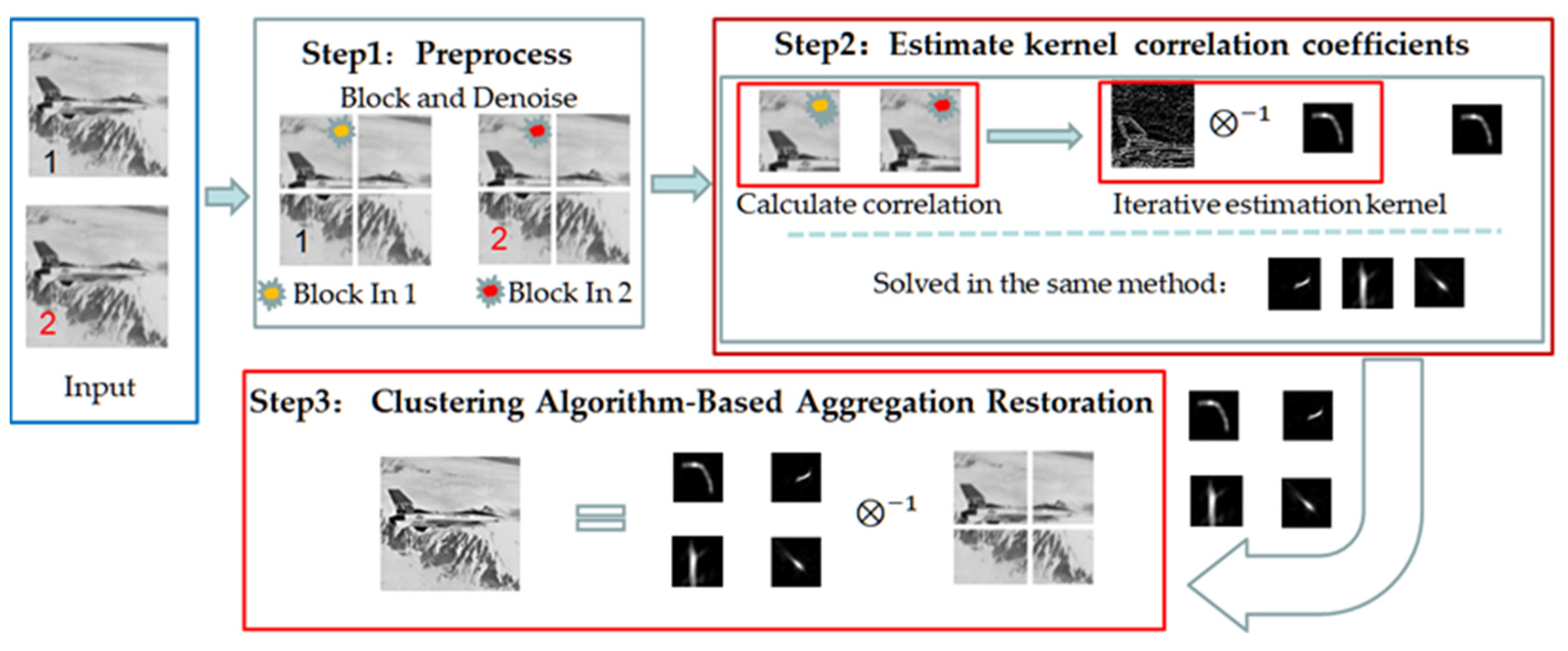
As shown in Figure 1, the work of Equation (2) was divided into three parts in this paper: (1) preprocess; (2) kernel estimation; (3) image restoration.

• Step 1: Preprocessing: De-noising, blocking, and building a pyramid of the input images

De-noise: In this paper, the image de-noising preprocess was performed using the currently widely used BM3D [12] algorithm. In the process of de-noising, balancing the image sharpness and signal-to-noise ratio after de-noising usually depends on empirical choices. In this paper, the blur kernel estimation process was mostly calculated in the gradient domain. Therefore, the presence of noise affected the sparsity of the gradient domain. Thus, the parameter settings for de-noising tended to enhance the de-noising effect, rather than protecting the image texture.

Block: In the process of image blocking, the size of the image blocks must be divided according to the size of the image and the forward step. The choice of block size and the length of the step are usually based on the nature of the image itself. If the similarity of the blur kernel-space change of the image is high, a relatively large step size can be chosen, to reduce the number of blocks and accelerate the calculation speed. If the space change shape is complex, a smaller block can be chosen, to improve the estimation accuracy [13].

Built pyramid: In common image deblur algorithms [2], an image pyramid is usually created by down-sampling in the process of kernel estimation. The kernel is estimated layer by layer, and the initial value of the next kernel is obtained by the up-sampling of the above layer result. The algorithm for estimating the kernel is the same for each layer in all blocks; therefore, the algorithm for the kernel estimation is presented in Section 3, as an example for any layer of any pair of image blocks.

• Step 2: Block layer kernel estimation (introduced in Section 3)

Section 3 introduces the kernel estimation method in any block layer of the image pyramid. For space-invariant image blurred images, where the whole image has the same blur pattern, calculating the RSPI block by block is equivalent to calculating the RSPI for the whole image. The specific reasons were described in the section on RSPI below. The split-block step can be omitted if dealing with space-invariant images. The blurring kernel of the whole image is estimated directly by building an image pyramid with the original image size as the initial value layer by layer.

With the dual-channel blurred images input, the RSPI between the sliced images was calculated using the total information from selected image blocks as a priori information. The image blur kernel was estimated and restored block by block.

This paper introduced the RSPI and WG-NGM to improve the accuracy of the block layer kernel estimation in the processes of block layer iter-kernel and block layer iter-image estimation.

The estimated kernel can be used to perform a deconvolution operation, to obtain a deblurred image. The image deblur model in the spatial domain was obtained from Equation (2):

$$X_1^{}=\underset{X_1^{}\in {\mathcal{X}}_1}{argmin }{‖H_1^{Total}⊛X_{{}_{iter}}^{Total}-Y_1^{Total}‖}_2^2+{\gamma }_X‖R(X_{{}_{iter}}^{Total})‖$$

(3)

${\gamma }_X$ is the regularization coefficient for an iter-restored image as a constant value, ${\mathcal{X}}_{opt}$ is the pool of allowed $X_{opt}$, $X_{{}_{iter}}^{Total}$ is the iter-image in the process, and $R(X_{{}_{iter}}^{Total})$ is the regularization term function for image restoration.

• Step 3: Blurred block image restoration (introduced in Section 4)

In Section 4, this paper focuses on a mean-shift clustering method, to collocate blocks of images that have been deblurred.

In this paper, we used the clustering method to determine the pixel values of overlapping regions when stitching together images. Depending on the weights of the kernels, the weights of the pixels in the corresponding image blocks are different. The final pixel value of the final deblurred image’s overlapping part is determined by deriving a weighted average.

3. The Block Layer Kernel Estimation

The main improvements of the proposed method in this section, which deals with the space-variant blurred images, are the modified regularization terms in the kernel estimation process.

Specifically, in the kernel estimation algorithm for each layer of the image block pyramid, this paper makes the following contributions:

•  In the block layer iter-kernel estimation process, using the RSPI of each pair of blocks to calculate the correlation coefficient, the integrity of the total information of the selected block was preserved to the greatest extent. Furthermore, the interference caused by the information from the other parts of the global image was avoided.
•  In the block layer iter-image estimation process, the advanced modified regularization term is proposed with the dual-channel images information introduced in this paper. With the improvements, the accuracy of the clock-layer kernel estimation was improved.

For the block layer kernel estimation problem, the estimation model from Equation (2) can be written in the following iterative form:

$$H=\underset{\nabla X\rightleftarrows h}{argmin}{‖h_{iter}⊛X_{iter}-Y_L‖}_2^2+{\lambda }_x‖T(X_{iter})‖+{\lambda }_h‖F(h_{iter})‖$$

(4)

where H is the result of the kernel estimation in this block layer, and $Y_L$ is the blurred image in this block layer, with it representing the alternate iterative minimization of the block layer iterative image $X_{iter}$ and the block layer iterative kernel. ${\lambda }_{{}_X}$ and ${\lambda }_h$ are regularization coefficients for iterative image estimation and kernel estimation in each block layer. $T(X_{iter})$ and $F(h_{iter})$ are regularization terms for the block layer iterative image estimation and layer-kernel estimation models, respectively. The choice of these coefficients is usually based on experience, depending on the design purpose of the regularization term and the characteristics of the image itself.

The design requirement of the regularization term $F(h_{iter})$ in the block layer iter-image estimation process aims to improve the reliability of the block layer iter-image. Regularization terms, such as the TV operator, are usually chosen to emphasize the gradient part of the blurred image. However, such features are derived from the gradient of the blurred image itself and lack reference side information to which to refer. Therefore, if the dual-channel blurred images are the input content with weak coprime, the two images will be more correlated. Furthermore, the more reliable information can be preserved using RSPI as the regularization term. In Section 3.1, this paper proposed a block layer iter-kernel estimation model with an RSPI regularization term for optimizing the block layer iter-kernel estimation process.

The design requirements of the regularization term $T(X_{iter})$ in the block layer iter-image estimation process usually need to consider the feature of the gradient image from the block layer iter-image. This paper introduced the side information from the input dual-channel corresponding image, to modify the regularization term NGM, which is used in [14]. The modified regularization term WG-NGM receives information from two-channel input images, making it more reliable than the NGM.

Therefore, through the improvements above, and by continuously iterating alternately to convergence, the optimal solution of the block layer kernel H can be obtained.

Finally, with the repetition of the up-sample and iterative solving process, the kernels of the blurred image blocks could be estimated.

3.1. The RSPI of Total Images

Generally, when the imaging results of the two channels are considered to be weak coprime, the morphological difference of the kernel is a constant, which changes its direction and size without changing its basic topology [9]. Therefore, assuming that the input two-channel image is weakly coprime, the ideal de-noising model of the blurred image can be obtained through the de-noise operation:

$$\begin{gathered} Denoise(Y_1^{Total})={DY}_1^{Total}=X⊛a_1\widehat{h} \\ Denoise(Y_2^{Total})={DY}_2^{Total}=X⊛a_2\widehat{h} \\ {H}_1^{Total}=a_1\widehat{h} \\ {H}_1^{Total}=a_2\widehat{h} \end{gathered}$$

(5)

The $\widehat{h}$ is the ideal shape of the kernel, $a_1$ is the deformation coefficient of kernel-1, $a_2$ is the deformation coefficient of kernel-2, and $Denoise()=D$ is the de-noise function.

The two equations in (5) can be combined to obtain:

$$(1/a_1){DY}_1^{Total}{⊛}^{-1}\widehat{h}=x=(1/a_2){DY}_2^{Total}{⊛}^{-1}\widehat{h}$$

(6)

The final result is:

$$(D(Y_1^{Total})-D(Y_2^{Total})){⊛}^{-1}\widehat{h}=0$$

(7)

With quadratic items:

$$R(\widehat{h})={‖(D(Y_1^{Total})-D(Y_2^{Total})\widehat{h}‖}_2^2$$

(8)

Even if using the quadratic term without de-noiseing: ${‖((Y_1^{Total})-(Y_2^{Total})\widehat{h}‖}_2^2$ as a regularization term, the result of the kernel estimation would be better than the regularization term of kernel’s norm-2: ${‖h_{temp}‖}^2$ [9]. Therefore, the correlation of the whole image is calculated with the condition of lower noise, and the result is more accurate [11]. Considering the convenience of using the sparsity of the gradient image to calculate the correlation coefficient, the correlation coefficient can finally be written as follows:

$$R_{\nabla }={\left[\nabla D(Y_1^{Total}),-\nabla D(Y_2^{Total})\right]}^T\left[\nabla D(Y_1^{Total}),-\nabla D(Y_2^{Total})\right]$$

(9)

“$\nabla$” signifies the function of the gradient operator, and $R_{\nabla }$ is the RSPI of the whole image.

In particular, it should be noted that if the blurred image is a space-variant blurred image, the step of split-block in the pre-processing is not required. The experimental part of this paper was devoted to testing the restoration of the space-invariant images, except for Group 4.

Furthermore, the problem that the algorithm in [11] faced is that the correlation coefficient just contains part of the information of the whole image, which is called the “effective part”, and would inevitably lose global information [15]. In the process of kernel estimation, if the kernel is calculated by the block method with the space-invariant blurred image, there is no need to consider the change of kernel morphology in the overlapping regions. This can be directly performed in simple equal-sized blocks. When the change of overlapping regions is not considered, the block operation actually introduces more edges that do not exist, and these non-existent edges will destroy the image’s smooth properties; this will lead to the appearance of unexpected ringing, which in turn affects the recovery of the image. As such, if the blurred image is a space-invariant blurred image, there will be a better restoration using the whole image to calculate the RSPI.

3.2. Block Layer Kernel Estimation: Applied RSPI and Weight-Balanced NGM (WG-NGM)

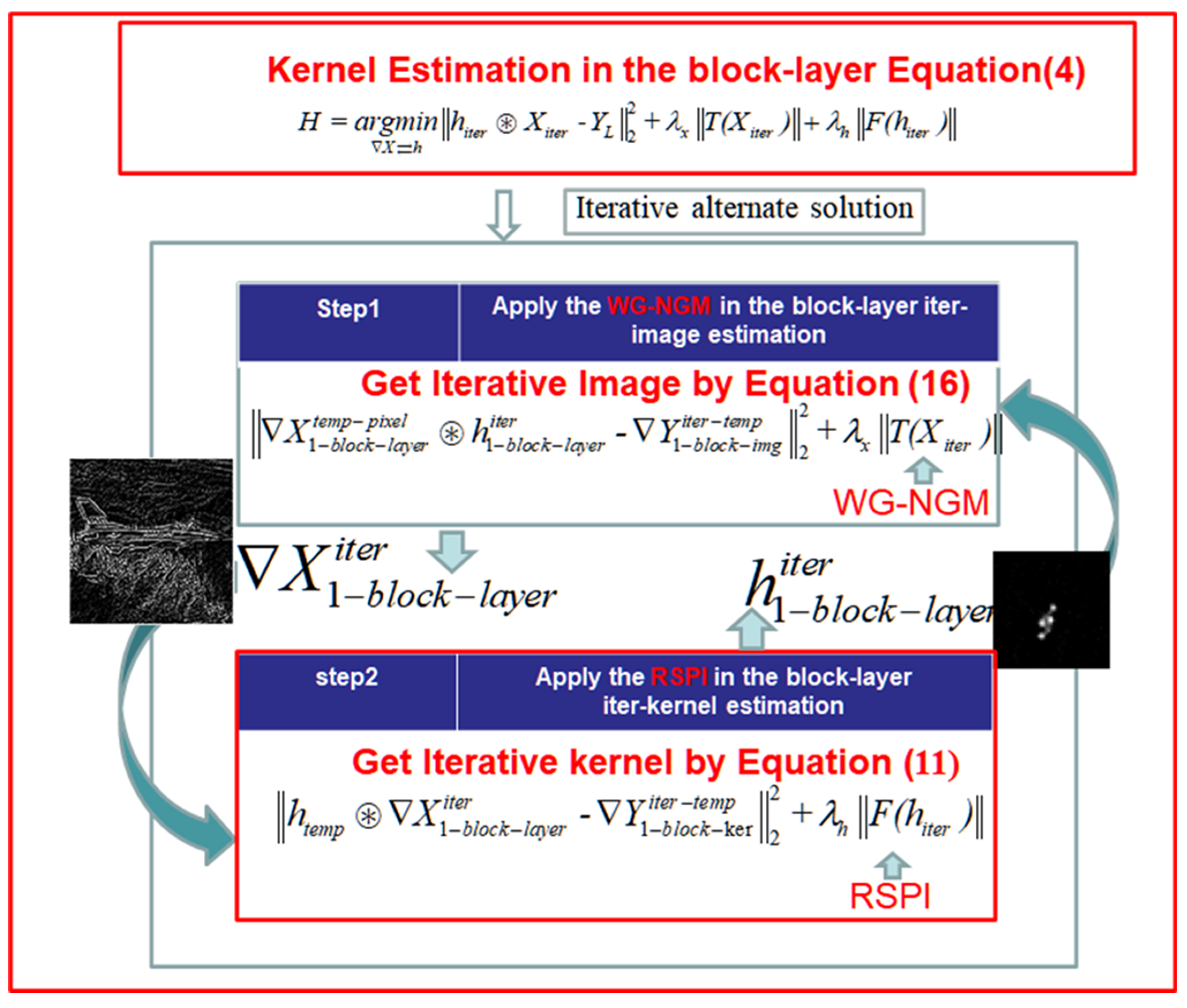
The kernel estimation problem is a non-convex underdetermined problem, so the method of using a gradient-like optimization algorithm to solve it often cannot obtain good results [16]. At present, the mainstream methods are based on the idea of the expectation-maximization (EM) algorithm [17], which estimates the iterative kernel and iterative image alternately. Based on the above framework, this paper proposed two regularization terms, which used RSPI and image correlation to improve the block layer iter-kernel and block layer iter-image estimation in space-variant image deblurring. The new method with the two regularization terms was found to enhance the accuracy of kernel estimation, as shown in

Table 1. Example of the method with RSPI.

	Length of Kernel	Angle	SSIM
RSPI	Len = 6	15, −60	0.9818
Norm_2			0.9764
RSPI	Len = 25	0, 90	0.9580
Norm_2			0.9416
RSPI	Len = 35	70, −150	0.9365
Norm_2			0.9334

and Figure 2. The specific processes and methods for kernel estimating are described below.

As previously mentioned, the proposed method builds an image pyramid by down-sampling and uses the same method to estimate the blur kernel at each layer.

As Figure 2 shows, the blur kernel estimation model Equation (4) for block layer images is divided into Equations (16) and (11), according to iterative image estimation and iterative kernel estimation, respectively. In addition, the iterative image and iterative kernel are estimated alternately using the EM method.

The block layer kernel estimation model in the gradient domain is obtained from Equation (2) as:

$$H_{{}_1}^{Total}=\underset{H_1{}^{Total}\in \mathcal{H}}{\arg \min }{‖h_{{}_{iter}}^{Total}⊛ (\nabla X_{}^{Total})-\nabla Y_{}^{Total}‖}_2^2+{\lambda }_h‖\varphi (h_{{}_{iter}}^{Total})‖$$

(10)

where ${\lambda }_h$ is the regularization coefficient of kernel estimation, $\mathcal{H}$ denotes the pool of allowed block layer kernel $H_1^{Total}$, $\varphi (h_{{}_{iter}}^{Total})$ is the regularization term function for kernel estimation as $F(h_{iter})$, and $h_{{}_{iter}}^{Total}$ is the temp iter-kernel in the process (same as $H_{}^{Total}$). Owing to its higher calculation efficiency [18], the kernel estimation model Equation (10) is solved in the sparsity gradient domain.

3.2.1. Block Layer Iter-Kernel Estimation with RSPI

First, the correlation coefficient of the two-channel image of this block-layer is calculated as RSPI: $R_{\nabla -block}=block({\left[\nabla D(Y_1^{Total}),-\nabla D(Y_2^{Total})\right]}^T\left[\nabla D(Y_1^{Total}),-\nabla D(Y_2^{Total})\right])$ (function block() means the area of the block in the whole images), and then the RSPI is applied to improve the block layer iter-kernel estimation model:

$$\begin{array}{c}{h}_{1-block-layer}^{iter}=\underset{h_{block-layer}^{iter}\in {\mathcal{H}}_{iter}}{\arg \min }({‖h_{temp}⊛\nabla X_{1-block-layer}^{iter}-\nabla Y_{1-block-\ker }^{iter-temp}‖}_2^2+{\lambda }_h{‖R_{\nabla -block}‖}^2{‖h_{temp}‖}_2^2)\\ s.t.{\displaystyle \sum h_{temp}^{pixel}}=1 and 1>h_{temp}^{pixel}\ge 0\end{array}$$

(11)

where 1 signifies channel-1, $h_{1-block-layer}^{iter}$ represents the block layer iter-kernel, ${\mathcal{H}}_{iter}$ denotes the pool of allowed block layer kernel $h_{1-block-layer}^{iter}$, $h_{temp}^{}$ represents the temp value of $h_{1-block-layer}^{iter}$ in the iterative kernel estimation process, $\nabla X_{1-Block-layer}^{iter}$ is the block layer gradient of the ideal image, $\nabla Y_{1-block-\ker }^{iter-temp}$ is the temp iteration blurred image’s block layer gradient image in the process, and $h_{temp}^{pixel}$ is each pixel of the $h_{temp}$.

Expanding this expression yields:

$$\begin{array}{l}\underset{}{h_{1-block-layer}^{iter}=\underset{h\in \mathcal{H}}{\arg \min }(}{h}_{temp}^T⊛(\nabla {\left(X_{1-block-layer}^{iter}\right)}^T\nabla \left(X_{1-block-layer}^{iter}\right)+{\lambda }_h{R}_{\nabla -block})\\ -h_{temp}^T\nabla {\left(x_{1-block-layer}^{iter}\right)}^T\nabla Y_{1-block-\ker }^{iter-temp})\\ s.t.{\displaystyle \sum h_{temp}^{pixel}}=1 and h_{temp}^{pixel}\ge 0\end{array}$$

(12)

It is easy to see that there are many ways to solve this problem, as [16] shows. However, the usual method of maximum a posteriori probability estimation (MAP) does not accommodate both the normalization and non-negativity conditions of the kernel in a single objective function. Therefore, this paper found a probability distribution that satisfies the multivariate Dirichlet distribution by variational estimation, to fit the real distribution of the kernel based on statistical theory. In this paper, the variational Dirichlet (VD) method was used to solve Equation (12) [3]; the gradient projection algorithm [3] was used to solve this problem. This method typically uses a given step-size minimum as the iteration termination threshold. Based on experience of selection, it is usually decided to terminate the iteration when the maximum number of iterations is 20 or when the relative change in the objective function is less than ${10}^{-5}$. The Dirichlet function for fitting the kernel is better than the other methods in its speed and accuracy of kernel estimation; for example, the gradient-like method and other functions (multivariate mixed Gaussian function etc.) to fit the kernel [3]. With the results obtained from the VD method, the block layer iter-kernel can be obtained.

Usually, the norm-2 of the kernel ${‖h_{temp}‖}^2$ is used as the regularization term in the estimation of the layer iter-kernel estimation [14]. Furthermore, it can be seen in Equation (11) that the computation of the ${‖h_{temp}‖}^2$ regularization term adds the unit matrix to the diagonal of the ${‖h_{temp}‖}^2$ result of the block layer iterated image. The essence of the RSPI operator involves introducing the two-channel image correlation to the ${‖h_{temp}‖}^2$ result of the block layer iterated image. Therefore, the use of RSPI instead of the ${‖h_{temp}‖}^2$ as the regularization term can effectively improve the kernel estimation accuracy.

As shown in Table 1, three sets of simulated blur images were obtained using images from the GoPro image library. The sizes of kernel were selected in sizes of (6, 6), (25, 25), (35, 35) pixels and blur angles of (15, −60), (0, 90), and (70, −150) degrees, respectively. The similarity index SSIM was chosen to examine the similarity between the RSPI and the ${‖h_{temp}‖}^2$ results in the kernel estimation process. The RSPI and ${‖h_{temp}‖}^2$ were used as the layer iter-kernel regularization terms $‖\varphi (h_{{}_{iter}}^{Total})‖$ in Equation (10):

$$\underset{}{\underset{h\in \mathcal{H}}{\arg \min }(}{h}_{temp}^T⊛(\nabla {\left(X_{1-block-layer}^{iter}\right)}^T\nabla \left(X_{1-block-layer}^{iter}\right)+{\lambda }_{h}I) -h_{temp}^T\nabla {\left(X_{1-block-layer}^{iter}\right)}^T\nabla Y_{1-block-\ker }^{iter-temp})$$

(13)

$$\underset{}{\underset{h\in \mathcal{H}}{\arg \min }(}{h}_{temp}^T(\nabla {\left(X_{1-block-layer}^{iter}\right)}^T\nabla \left(X_{1-block-layer}^{iter}\right)+{\lambda }_h{R}_{\nabla -block}) -h_{temp}^T\nabla {\left(X_{1-block-layer}^{iter}\right)}^T\nabla Y_{1-block-\ker }^{iter-temp})$$

(14)

and used with the same NGM term in the layer iter-image (without blocking because of un-space-variation).

It can be seen that the RSPI results were more similar than the norm-2 ${‖h_{temp}‖}^2$ results, except that the blurred kernel vectors were in quadrants 1 and 3, respectively (the advantage was, therefore, not obvious).

3.2.2. Block Layer Iter-Image Estimation with WB-NGM

As mentioned above, the ordinary regularization term NGM was improved upon with the WB-NGM. As shown in Figure 2, the ${\lambda }_2\left|\nabla X_{2-block-layer}^{iter-pixel}\right|$ from channel-2 of the proposed WG-NGM method was found to effectively improve the texture restoration effect of the iterative image and improve the restoration accuracy of the iterative kernel.

The calculation method of WB-NGM is as follows:

$$T(X_{iter})=\frac{\left|\nabla X_{1-block-layer}^{iter-pixel}\right|}{\left|{\lambda }_1\left|\nabla X_{1-block-layer}^{iter-pixel}\right|+{\lambda }_2\left|\nabla X_{2-block-layer}^{iter-pixel}\right|\right|+E\left[\nabla Y_{1-block-img}^{iter-temp}\right]}$$

(15)

where $E\left[\nabla Y_{1-block-img}^{iter-temp}\right]$ indicates the mathematical expectation operation performed on the channel-1 iterative blurred block layer image gradient map $\nabla Y_{1-block-img}^{iter-temp}$ in the block layer iter-image estimation process, and the value is the mean of the gradients of all pixels of the $\nabla Y_{1-block-img}^{iter-temp}$. $\nabla X_{1-block-layer}^{iter-pixel}$ and $\nabla X_{2-block-layer}^{iter-pixel}$ are the pixel values of the selected location in the gradient images of the block layer iter-images from channel-1 and channel-2. ${\lambda }_1$ and ${\lambda }_2$ (determined by experience) are weighting factors to control the ratio of two pixels. If the located pixel’s gradient value $\nabla X_{1-block-layer}^{iter-pixel}$ is larger than the $E\left[\nabla Y_{1-block-img}^{iter-temp}\right]$, the pixel is retained; otherwise, it is discarded. By updating the threshold and iterative formula repeatedly, only small parts of the pixels are retained in the final result, which improves the accuracy of the blur kernel estimation, while ensuring sparsity.

The WG-NGM could be applied to rewrite the block layer iter-image model as:

$$\begin{array}{l}\underset{}{\nabla X_{1-block-layer}^{iter}=argmin(}{‖\nabla X_{1-block-layer}^{temp-pixel}⊛h_{1-block-layer}^{iter}-\nabla Y_{1-block-img}^{iter-temp}‖}_2^2\\ +{\lambda }_x\frac{\left|\nabla X_{1-block-layer}^{iter-pixel}\right|}{\left|{\lambda }_1\left|\nabla X_{1-block-layer}^{iter-pixel}\right|+{\lambda }_2\left|\nabla X_{2-block-layer}^{iter-pixel}\right|\right|+E\left[\nabla Y_{1-block-img}^{iter-temp}\right]})\end{array}$$

(16)

To solve this problem, this paper used an iterative shrinkage-threshold (abbreviated as IST) algorithm [19], which has a good restoration effect for the non-uniform kernel. The WG-NGM can be thought of as a norm-1 regularization term. The IST algorithm typically uses the given maximum number of iterations or the difference between the target values of the two iterations as the threshold critical. In this paper, the maximum number of iterations was set to 10 times, based on the design experience in the references, and the minimum threshold was ${10}^{-2}$.

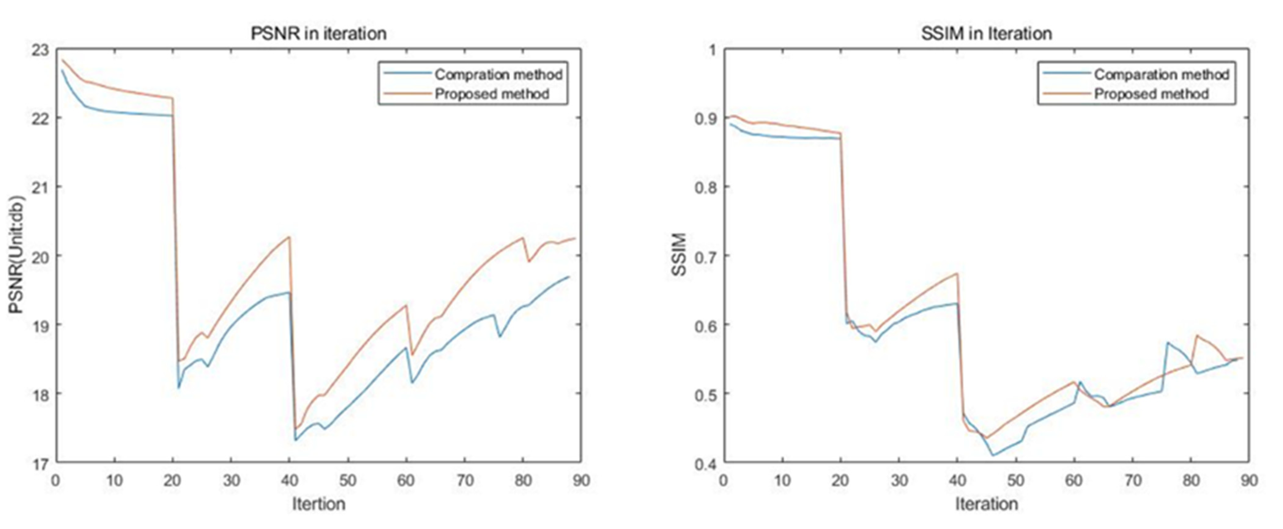
In order to verify that the introduced multi-channel information could improve the estimation of iterative images, two images from the Levin image set were selected for testing in this paper.

As shown in Figure 3, it was found that the iterative results estimated by the WG-NGM term performed better than those estimated by the NGM term (the different scales caused the step-like performance in the image pyramid, as Figure 3 shows, because the smaller images had a better performance). The data were displayed for approximately 90 iterations (the pyramid was divided into nine layers, and the number of iterations estimated for each layer of the iterative image was ten, so there were 90 iterations), which was in line with the results of the Group-1 experiment below.

The same parameters were used to create a pyramid of images of the same size as the baseline. The performance of the WG-NGM and NGM algorithms was compared separately to the iterative images for 90 iterations. PSNR and SSIM were chosen as the test indicators.

As the figure shows, the WG-NGM method performed better in terms of PSNR, and the final three results in the SSIM were compared, as follows:

The value of SSIM is usually small, so the difference in the final stages in the Figure 3 appears to be small.

Table 2. Final results of SSIM.

WG-NGM	0.5498	0.5509	0.5519
NGM	0.5415	0.5474	0.5488

lists the comparison of the SSIM values of the last three terms of the two methods. It can be noticed that WG-NGN performed better.

Therefore, it was demonstrated that the WG-NGM term can effectively improve the accuracy of the existing algorithm.

4. Blocked Image Restoration Based on Clustering Algorithm

The main improvement of the proposed method in this section, which deals with space-variant blurred images, is the block strategy, which is based on the mean-shift method to restore large-scale blurred images.

In space-variable blurred images, the kernel of each block is different [13]. Therefore, it is necessary to fully consider the selection of pixel values in the overlapping area in the process of restoring image block stitching. It is hard to obtain a good kernel estimation result, due to the weak intensity of the texture edge in some parts of images. Furthermore, if the blocks are derived from different blurred transition regions, the results of estimating the blur kernels have no valuable reference significance area. Therefore, if the mean value of the corresponding pixels in the relevant blocks is used as the corresponding pixel value of the restored image directly, the result is inaccurate [13]. To solve these problems, this paper used a kernel classification technique based on the mean-shift clustering algorithm [13] to distinguish high-weight kernels from low-weight kernels. In the final step of stitching, the value of the corresponding pixel was determined according to the quality weight of the blur kernel. The restoration of the final image has three main components:

•  Block image restoration

As mentioned above, if the blurred images are all divided into $N$ groups horizontally and $M$ groups vertically, for a total of $N\times M$ blocks, the number of corresponding kernels is also $N\times M$. First, this paper used the kernel of each block to restore the corresponding block of the images separately. For each blur kernel $Kerne{l}_i$ (i means the order of the kernel, and $i\in N\times M$), the alternating direction method of multipliers (ADMM) [20] algorithm was applied to restore the block of blurred images corresponding to that kernel.

2.

 Mean-shift cluster weight calculation

In the process of image restoration, the determination of the pixel values of the overlapping parts of the image blocks is an important part of image deblurred. The method used in this paper requires all the weights of the image blocks. The weights are used in determining the rate of value in the final recovered image from each image block. Generally, the more blur kernels that have a similar blur form, the more pixels in the whole image that are blurred according to that blur pattern. Therefore, this paper used a mean-shift clustering algorithm to classify the blur kernels and finally obtain a clustering result where the blur kernels are classified according to similarity as the flow shown in

Table 3. The flow of the mean-shift cluster method in kernel categorization.

Mean-Shift Cluster Method in Kernel Categorization
Step 1:  Calculate the pixel sum of squares for each kernel as its weight:                 $Weigh{t}_i={\displaystyle \sum _{n,m}{‖Kerne{l}_{pixel}^i‖}^2}$
Step 2:  $\mathrm{Taking} \mathrm{the} Weigh{t}_S$$\mathrm{as} \mathrm{the} \mathrm{center} \mathrm{value} \mathrm{of} \mathrm{the} \mathrm{cluster}{C}_s$ $\hspace{1em}\hspace{1em}\hspace{1em}\hspace{1em}\hspace{1em}\hspace{1em}{C}_s=\left\{Weigh{t}_{S-C}\right\};Weigh{t}_{S-C}\in Kernel(Weight<Band)$
Step 3:  $\mathrm{Taking} \mathrm{the} Weigh{t}_S$$\mathrm{as} \mathrm{the} \mathrm{center} \mathrm{value} \mathrm{of} C_s$  Calculate the sum of all the vectors:              ${\overrightarrow{D}}_{sum}={\displaystyle \sum _{j\in S-C}{\overrightarrow{D}}_j};{\overrightarrow{D}}_j=Weigh{t}_j-Weigh{t}_S$
Step 4:  $\mathrm{Calculate} \mathrm{the} \mathrm{new} \mathrm{center} Weigh{t}_{new}$$\mathrm{with} \mathrm{the} {\overrightarrow{D}}_{sum}$:              $Weigh{t}_{new}=Weigh{t}_S+{\overrightarrow{D}}_{sum}$  $\mathrm{Add} \mathrm{all} \mathrm{the} \mathrm{kernels} \mathrm{which} \mathrm{weigh} \mathrm{less} \mathrm{than} {\overrightarrow{D}}_{sum}$$\mathrm{in} \mathrm{the} \mathrm{cluster} C_s$
Step 5:  If  $Weigh{t}_{new}-Weigh{t}_s<{\overrightarrow{D}}_{sum}$  do:   two clusters can be merged  else   A new cluster should be obtained
Step 6:   Run step 3   $\mathrm{Until} {\overrightarrow{D}}_{sum}<t$ (t as selected by the experiment)
Step 7:  Run step 2 Until all the kernels are visited

.

$Weigh{t}_i$ denotes the weight of the i-th kernel, $i\in N\times M$ is the order number of the kernel, $n,m$ are the length and width of the kernel (unit: pixel), and ${‖Kerne{l}_{pixel}^i‖}^2$ means the sum of squares for all pixel values in the kernel, $C_s$ is the cluster of all the kernels (representative weight value as $Weigh{t}_{S-C}$ for all of them) whose absolute values of the difference between their weight values are less than a threshold (names $Band$ in follow, which was determined by experience), ${\overrightarrow{D}}_j$ is the weight vector for the difference of the j-th kernel’s weight in the cluster $C_s$, the pool of j is the element’s order number in $C_s$, and $Weigh{t}_{new}$ is the new center.

3.

 Each pixel’s value from the sum of the normalized weights

For computational convenience, all image blocks should be complemented first. For example, if the original image size was 800 × 800 and the image block size was 200 × 200, fill in zeros around the image block according to its position on the original image, until it is the same size as the original image; 800 × 800 as layer-recovered images. Then, the value of the pixels in the final restoration image was determined by all values from the same location pixels in all layer-recovered images. The weight of layer-recovered images was calculated using the ratio of the total element number of the corresponding kernel’s class to the total number of kernels. For example, if there are two kernels that have similar forms in one cluster and the total number of kernels is 8, then the weight of the pixels in the blocks recovered by the two kernels is 0.25.

The calculation of the pixels’ value of the final restoration image was performed as follows:

$$X_{pixel}={\displaystyle \sum _{k\in {\Omega }_c}{\lambda }_k(X_{layer}^{k-pixel})}$$

(17)

$X_{pixel}$ denotes the selected pixel’s value for the final restoration image $X$. ${\lambda }_k$ means the weights of the k-th kernel, $X_{layer}^{k-pixel}$ signifies the same selected location pixel value as the k-th layer-recovered image, and ${\Omega }_c$ means all of the layers recovered images.

5. Experimental Results

To verify the restoration effect of the proposed algorithm, three groups of experiments were used for verification. The Group-1 experiments were simulation experiments with simulation data; the Group-2 experiments involved real-shot image restoration with space-invariant images; and Group-3 were real-shot experiments with space-variant images. The three groups of experiments verified the practicability of the algorithm by comparing the restoration results of the Levin Library, sample images provided by other literature, and our images. Among them, the simulated images sets were quantitatively analyzed through a variety of indicators, and the real-shot images sets were generally selected to use the method of visual observation to evaluate the restoration quality. Moreover, the results from [11] (code download on http://zoi.utia.cas.cz/download_toolbox (accessed on 28 May 2020) with permission) and [14] (code used with GNU) were calculated using the copyright permission when the software was downloaded. Group-4 used space-variance blurred images of the target plate to test the recoverability of this method.

All programs were running on the student version of MATLAB 2017 under the licensed Windows 11 platform. The CPU was an Intel Core i7 8750H, and 32G memory with Intel 750 SSD. Peak signal-to-noise ratio (PSNR, unit: dB) and structural similarity index (SSIM) were calculated using MATLAB’s functions, with default parameters.

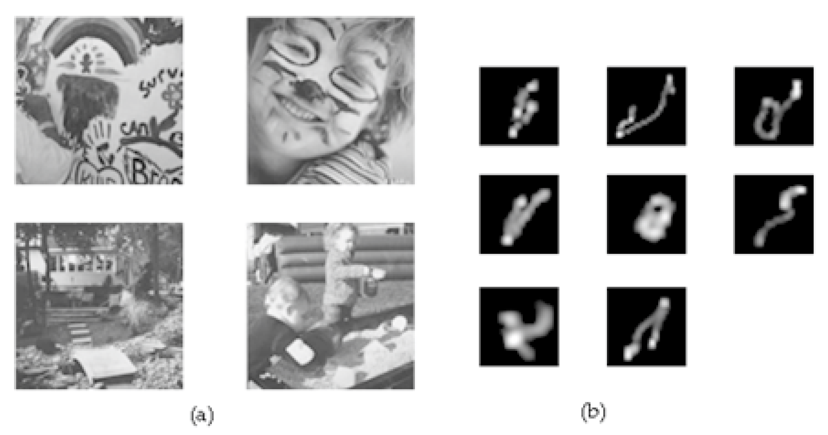
Group 1: In this group, the non-space-variant blurred images of the Levin image library were used to compare and test the restoration ability of the algorithm for non-space-variant blurred images. This group mainly verified the estimation ability of the algorithm to the kernel, so we chose to compare all 32 results from the total of four original images and eight kernels. The comparisons were obtained from the studies by Xu et al. [14,21,22,23]. The codes of those papers were downloaded from their official websites on GitHub, with a GPL or GNU open-source license. The comparison method also used the PSNR and SSIM to measure the results from the two algorithms. The total images, and kernels are shown in Figure 4, and the results are shown in Figure 5.

Furthermore, the results of [21,22,23] were provided by their official GitHub site. The results were not obtained by the authors of this paper running the program on this machine, except running times or special declarations.

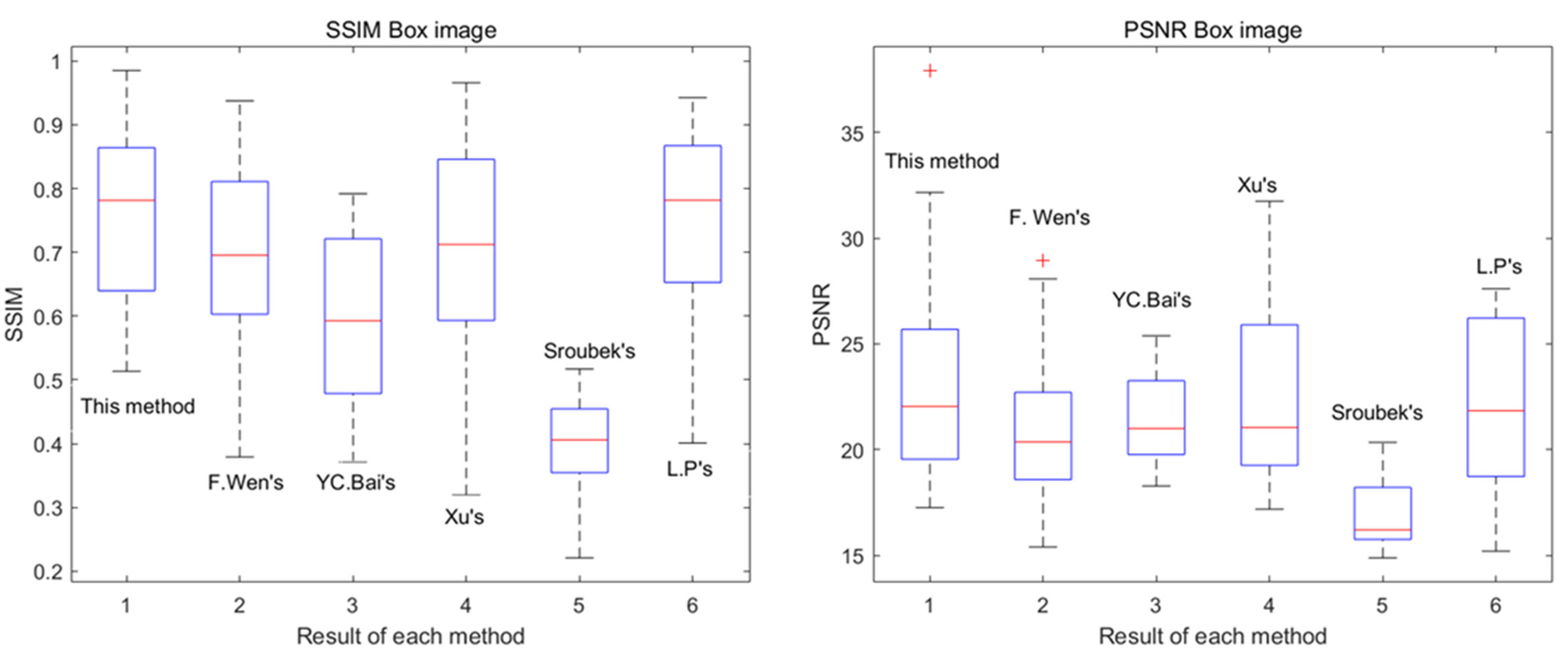
Figure 4a shows the original images and Figure 4b the self-designed simulation blur kernel. Figure 5 shows all the results obtained when simulations were performed in two-by-two teams in the order of images and blur kernels. It can be seen that the proposed algorithm performed well overall, in terms of the PSNR and SSIM.

Discussion: As shown in Figure 5, with the PSNR, this algorithm not only produced a result up to 35+, but the mean and the concentration of the distribution interval of the PSNR of this algorithm were higher than the other algorithms. Moreover, the lower bound of this algorithm in the PSNR was higher than the others.

The proposed algorithm also performed well in for the SSIM. It led, both in terms of the maximum and mean values, and the lower bound of the interval.

This shows that the recovery results of this method are more stable overall, with less variation in the results for images with different blurring patterns. Moreover, with stability and balance, this method provided the highest performance results and high lower bounds. It is also worth mentioning that, since the Levin library is a space-invariant blurred image simulation library, this algorithm does not fall short in terms of time consumption. The time cost of the remaining algorithms was essentially close, except for the frequency domain-based L.P’s algorithm, which has a significant advantage over the present algorithm as

Table 4. Restoration quality evaluation table of times.

Indicators	Proposed	Sroubek	Xu	YC.B	F.Wen	L.P
Times (Unit: s)	27.33	43.02	17.19	27.24	23.19	12.96

shows.

Group 2: In this group, two sets of test images from the literature [11] were used as the test objects. The first set of photos in this group were real images without the original, and the second set were real-shot images.

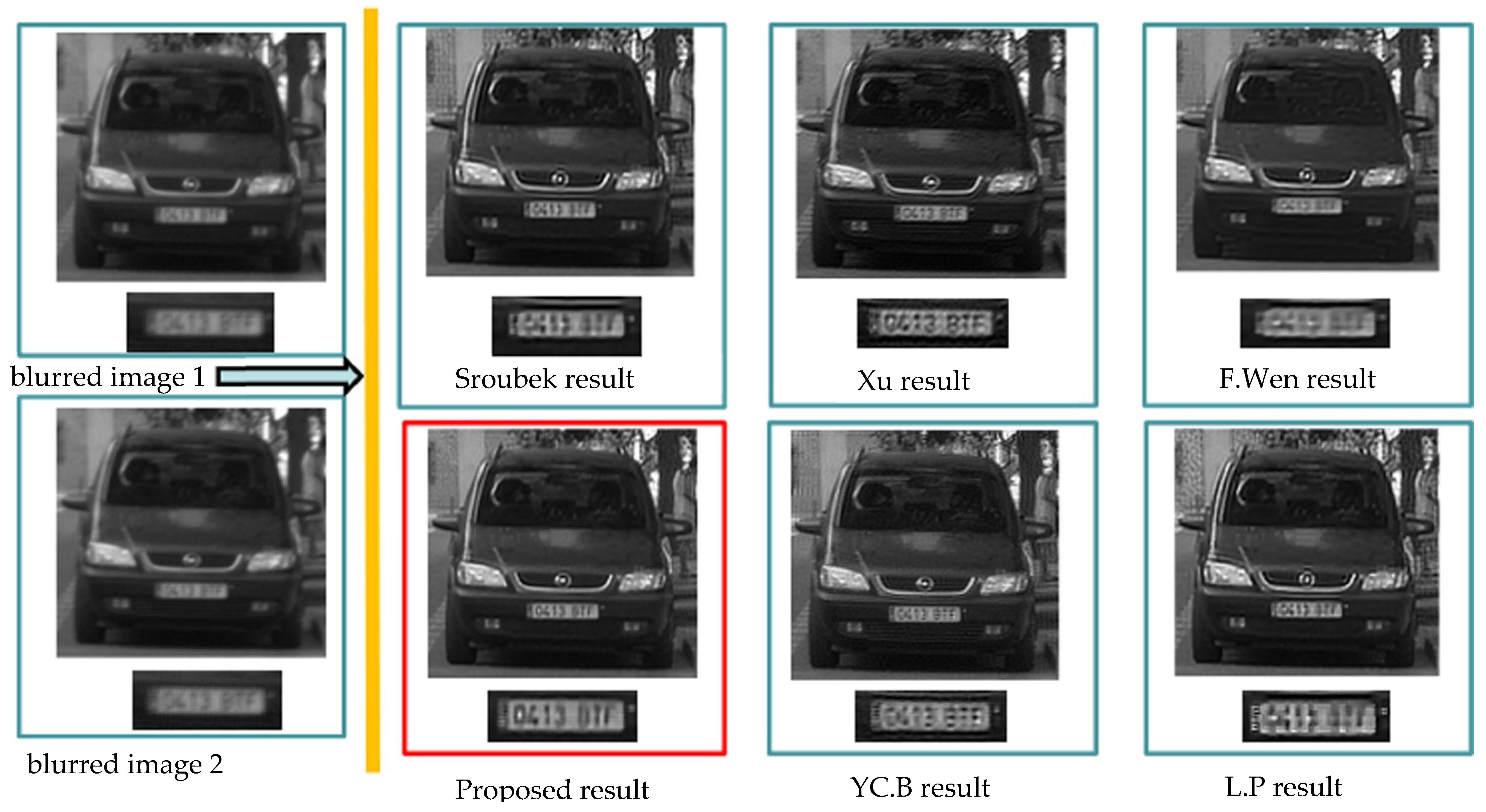
Set 1 Discussion: The images in this set are real images provided from the open-source algorithm by Mr. Sroubek’s official website. There is no original image, so the PSNR and SSIM cannot be used to test the restoration. Fortunately, in this paper, it is not too difficult to obtain meaningful visually observed results.

Looking at the details of the license plate in Figure 6, it can be seen that both Xu’s algorithm and YC. B’s algorithm [22] can roughly identify the character B. The proposed method could identify the number. The main reason for this difference is that both the Xu’s and YC. B’s algorithms had a certain ringing effect, so in the recovery results there are some horizontal stripes in the middle of the plate, which unexpectedly enhance the recognition of the letter B. Therefore, on balance, the proposed algorithm had a better performance in removing ringing and recovering the details of the numbers.

Set 1:

Figure 6. Sroubek’s sample restored experiment set1. On the left, the top image is the blurred image1, and the blurred image 2 is at the bottom. In the top from left to right, is the Sroubek’s result, Xu’s result, and F.Wen’s result; the bottom list, from left to right, shows the proposed method’s result, YC.B’s result, L.P’s result.

Figure 6. Sroubek’s sample restored experiment set1. On the left, the top image is the blurred image1, and the blurred image 2 is at the bottom. In the top from left to right, is the Sroubek’s result, Xu’s result, and F.Wen’s result; the bottom list, from left to right, shows the proposed method’s result, YC.B’s result, L.P’s result.

The proposed method provided a good recovery result. Although slightly worse in terms of horizontal image features, it avoided more ringing in the whole image. In addition, the proposed method also recovered the numbers in the license plate clearly, which shows that this method has better generalizability, rather than good recovery for specific targets.

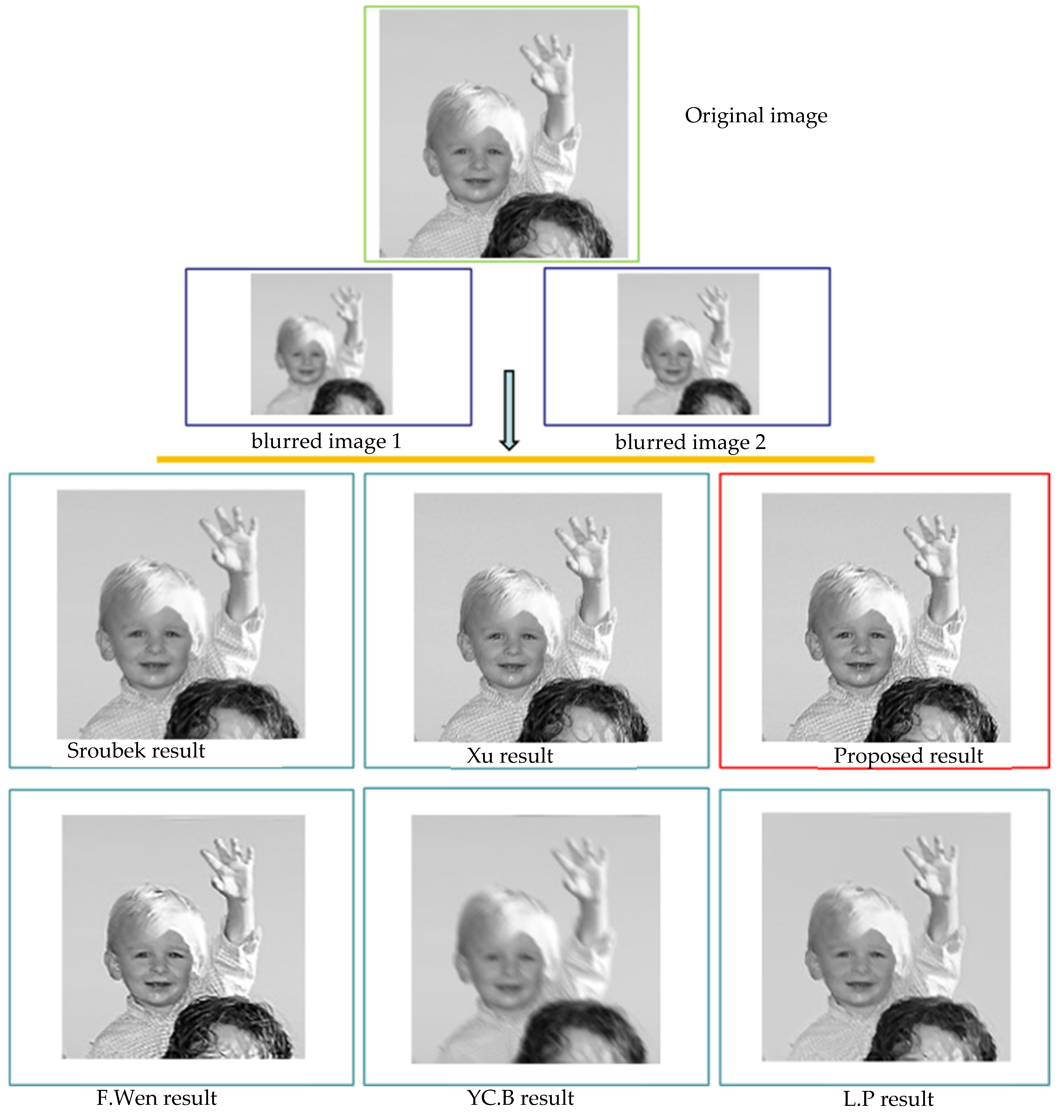
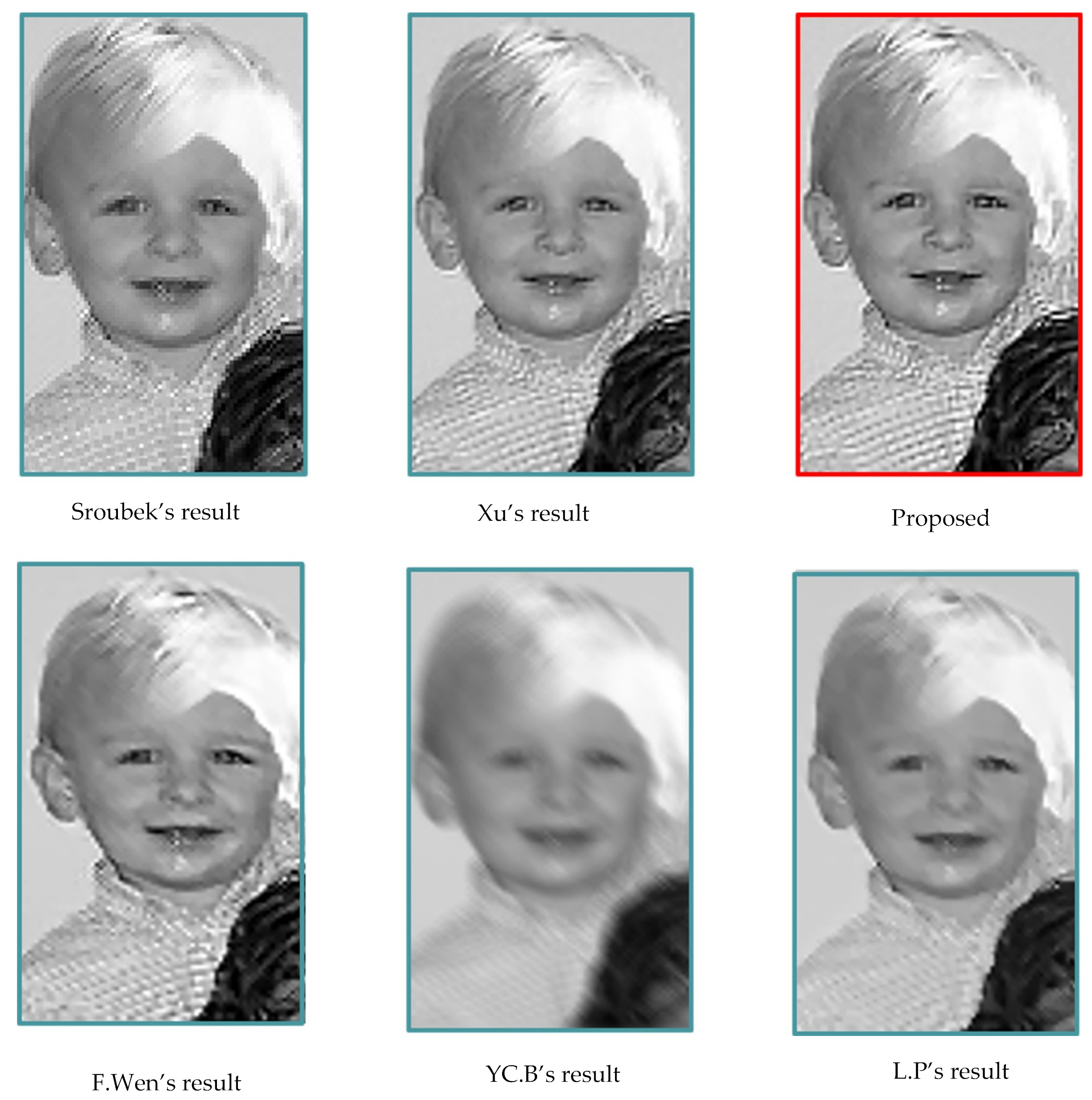
Set 2 Discussion: From the directed observation in Figure 7, the proposed algorithm performed better. For example, the checkered texture of the clothes on the left shoulder, and the texture of the face in Figure 8. Moreover, the image recovered by the proposed method is sharper and has more details than the original image size.

Both the PSNR and SSIM mean that the algorithm has a leading location in Table 5. It is worth noting that the F. Wen’s algorithm achieved better results, both in the Levin library and in Sroubek’s image library. Therefore, the next set of experiments, represented by the F. Wen’s method, tested the effectiveness of the present algorithm on a color image.

Set 2:

Figure 7. Sroubek’s sample restored experiment set 2. In the top line, it is the original image; the second line shows the input blurred images 1 and 2; the third line, from the left to right, are the results of Sroubek, Xu, and the proposed method; the fourth line, from the left to right, are the results of F.Wen, YC.B, and L.P.

Figure 7. Sroubek’s sample restored experiment set 2. In the top line, it is the original image; the second line shows the input blurred images 1 and 2; the third line, from the left to right, are the results of Sroubek, Xu, and the proposed method; the fourth line, from the left to right, are the results of F.Wen, YC.B, and L.P.

Figure 8. Sroubek’s sample restored experiment set 2 details. At the top, from left to right, are the results of Sroubek, Xu, and the proposed method; The next line, from left to right, shows the results of F.Wen, YC.Bai, and L.P.

Figure 8. Sroubek’s sample restored experiment set 2 details. At the top, from left to right, are the results of Sroubek, Xu, and the proposed method; The next line, from left to right, shows the results of F.Wen, YC.Bai, and L.P.

Table 5. Restoration quality evaluation table of Sroubek’s set2.

Indicators	Proposed	Sroubek	Xu	YC.Bai	F.Wen	L.P
PSNR	27.64	25.47	26.23	23.21	13.62	26.81
SSIM	0.8572	0.8317	0.8572	0.8348	0.7469	0.7947

Table 5. Restoration quality evaluation table of Sroubek’s set2.

Indicators	Proposed	Sroubek	Xu	YC.Bai	F.Wen	L.P
PSNR	27.64	25.47	26.23	23.21	13.62	26.81
SSIM	0.8572	0.8317	0.8572	0.8348	0.7469	0.7947

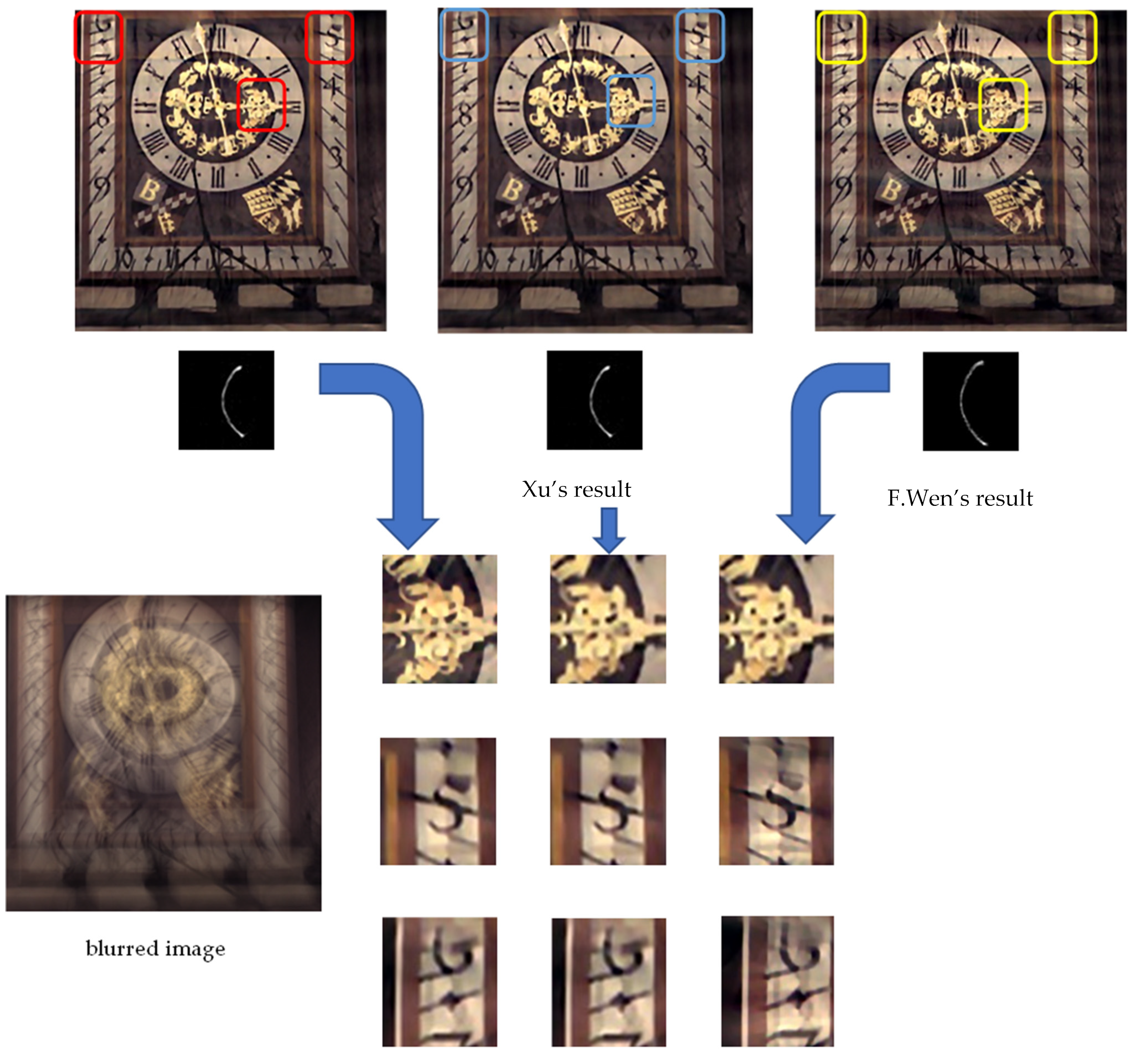
Group-3: The eighth blur image of the bell, one of the most difficult image to deblur in the Kohler library, was chosen to test the proposed method’s ability for blurred color image restoration, and shown in Figure 9 and

Table 6. Restoration quality evaluation table of Kohler’s bell.

Evaluation Object	Indicators	F.Wen	Xu	Proposed
Restoration results	PSNR	11.8610	11.5741	11.9056
	SSIM	0.3683	0.3790	0.3825

. Since the results of these images are only provided in the open-source code of F. Wen’s program, without other methods, this experiment only examined the proposed algorithm’s results, which were compared to Xu’s and F.Wen’s results.

Discussion: The F. Wen method’s official code provided the recovery results for this image directly. Using the recovered images provided by the code was as objective and fair way to compare with the proposed method’s result. Looking at the whole image, the algorithm in this paper consistently performed well in dealing with the ringing effect. In the detail section, whether it was the pointer in the table or the numbers and letters, the results recovered by this algorithm were clear in detail. The blur kernels of the image show that the curvature of the blur kernels estimated by this paper’s algorithm was more rounded, and the energy distribution of the blur kernels at the ends is greater. It avoided the more horizontal bar seen with the F. Wen algorithm. In terms of PSNR and SSIM, the algorithm in this paper also maintained the lead. Moreover, from the experimental results provided in F.Wen’s study, F.Wen’s method is the one of best methods for space-invariant color deblurring in both the Levin and Kohler libraries. Combined with the experimental results of Group-2, it was proven that the proposed method has a better performance in processing black and white images and color images.

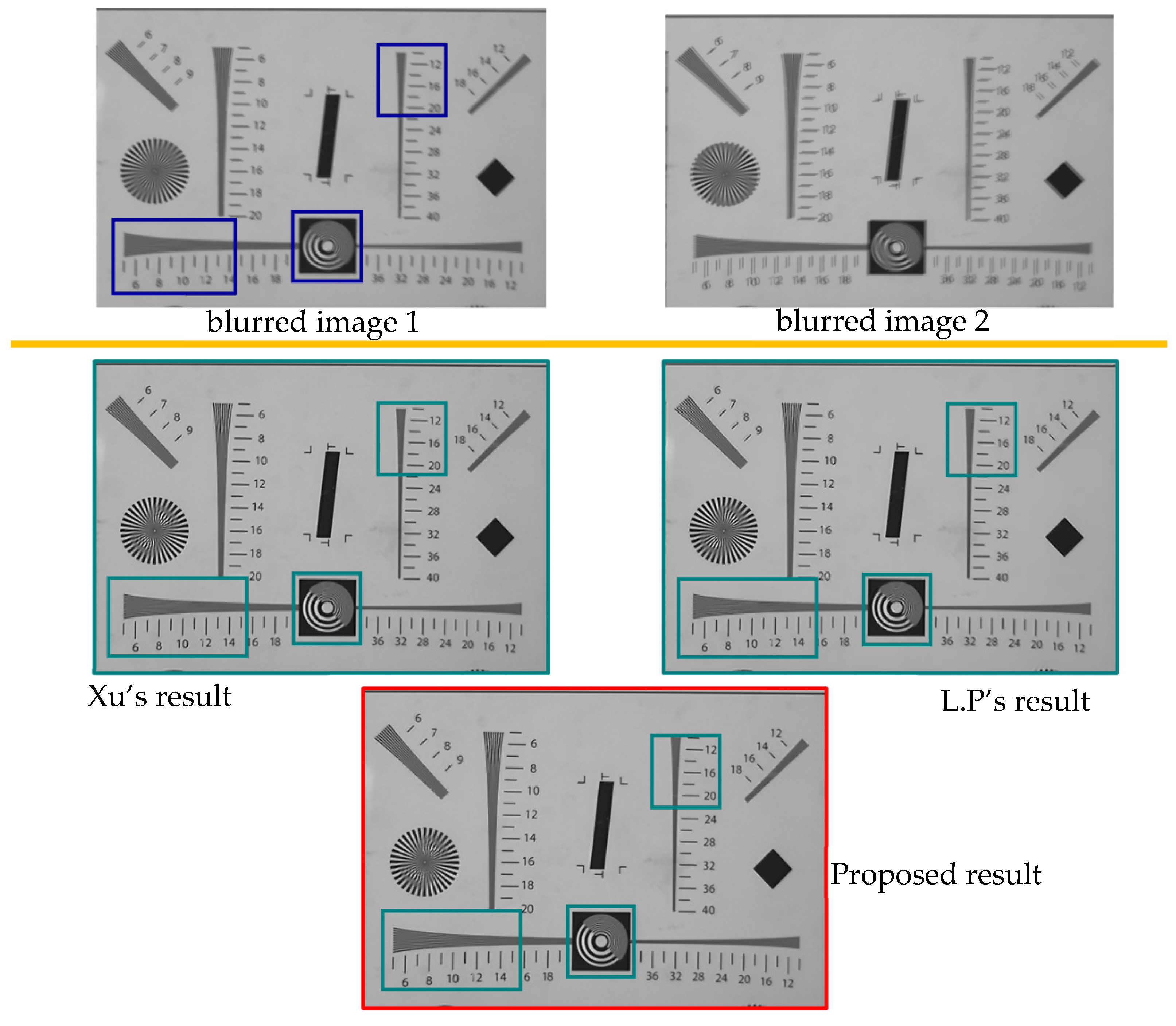
Group-4: Group-4 aimed to verify the restoration effect of large-scale space-variant images. Images were taken with an industrial camera “Imaging-Source DFK290”. The imaging parameters of the two images were set the same: the exposure time was 1/66 s, the ISO was 240, the length and width of a single CMOS pixel were both 3 microns, the focal length was 5 mm, and the object distance was 75 cm. The resolution of the image was 1920 × 1080 (unit: pixel), and the area of the target plate was 800 × 550 pixels in the image used. The images were preprocessed for registration and brightness matching before use. The object of the target plate was designed using ISO122333 [24] standards. The measurement algorithm implemented the calculation by selecting the program (SFR_1.41) compiled by MITRE Corporation in 2006.

This group of experiments comprised real-shot experiments, so the subjective evaluation method was used to evaluate the restoration quality of the images. However, some existing image quality assessment (IQA) indicators were also used, such as the natural image quality evaluator (NIQE: the smaller the value, the smaller the gap with the natural image, and the better the image quality [25]), and the average gradient (the larger the value, the clearer the image texture). These two indicators were, thus, able to evaluate the image restoration quality from other perspectives.

The comparison methods were L.P’s and Xu’s methods. The main reason for not choosing other methods was because other algorithms were more complicated to set up and had less reference value for the results run on the local machine. Moreover, the L.P’s algorithm was more advanced, as seen in previous comparisons of works with space-variation images. Thus, the open-source program required only one major parameter, kernel size, so the results of L.P’s method were more reliable if computed on this machine.

The results are shown below in the order:

• The restoration of whole images in Figure 10;
• The kernel result and the MFT in Figure 11;
• The details of restoration in Figure 12;
• The IQA of the results in

  Table 7. Final results of the IQA.

  Test Image	Evaluation Criterion	Xu	L.P	Proposed Algorithm
  Plate	NIQE	4.1217	4.6578	3.9489
  	Average Gradient	5.7576	5.3857	5.8725

  ;

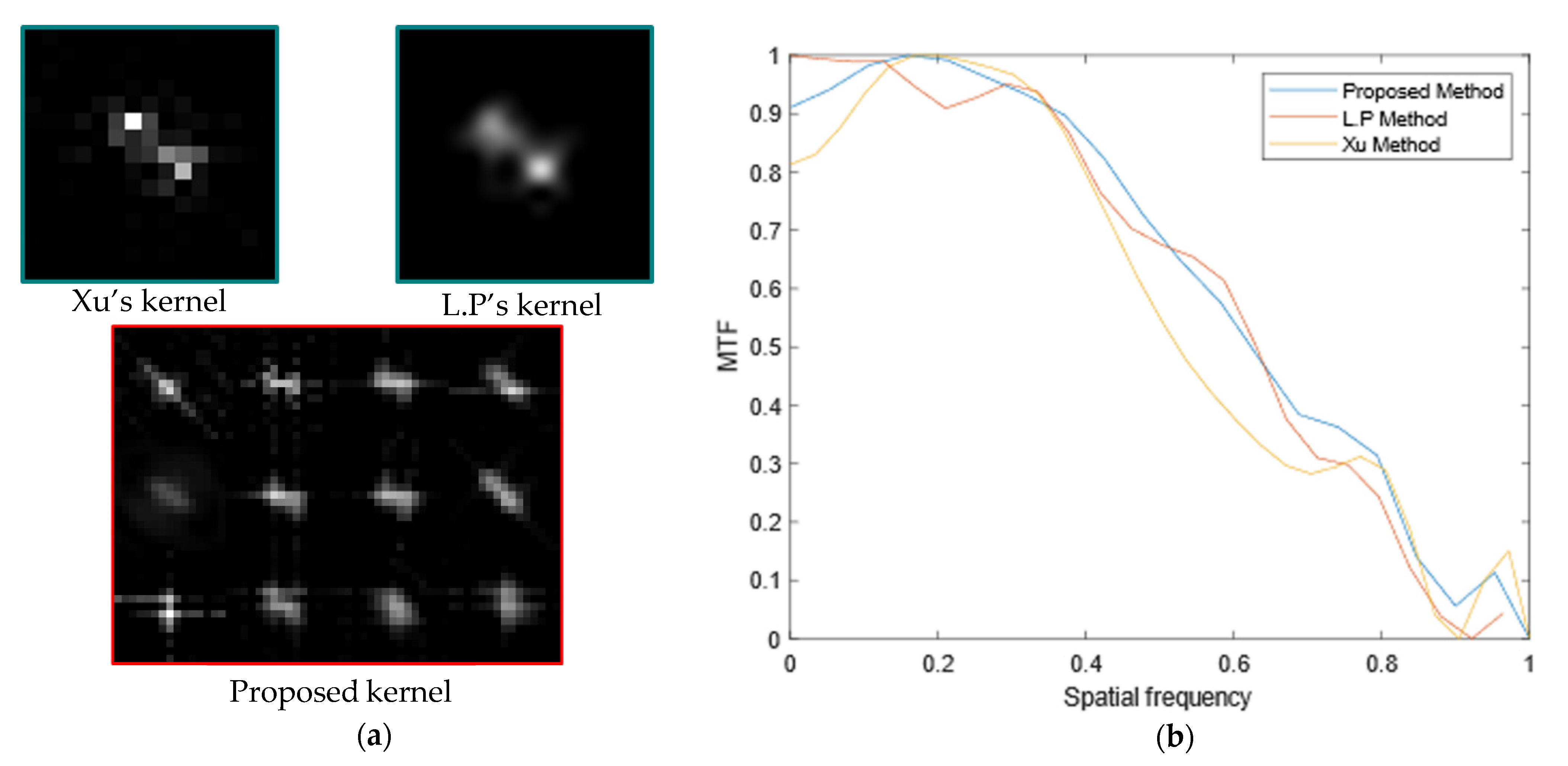
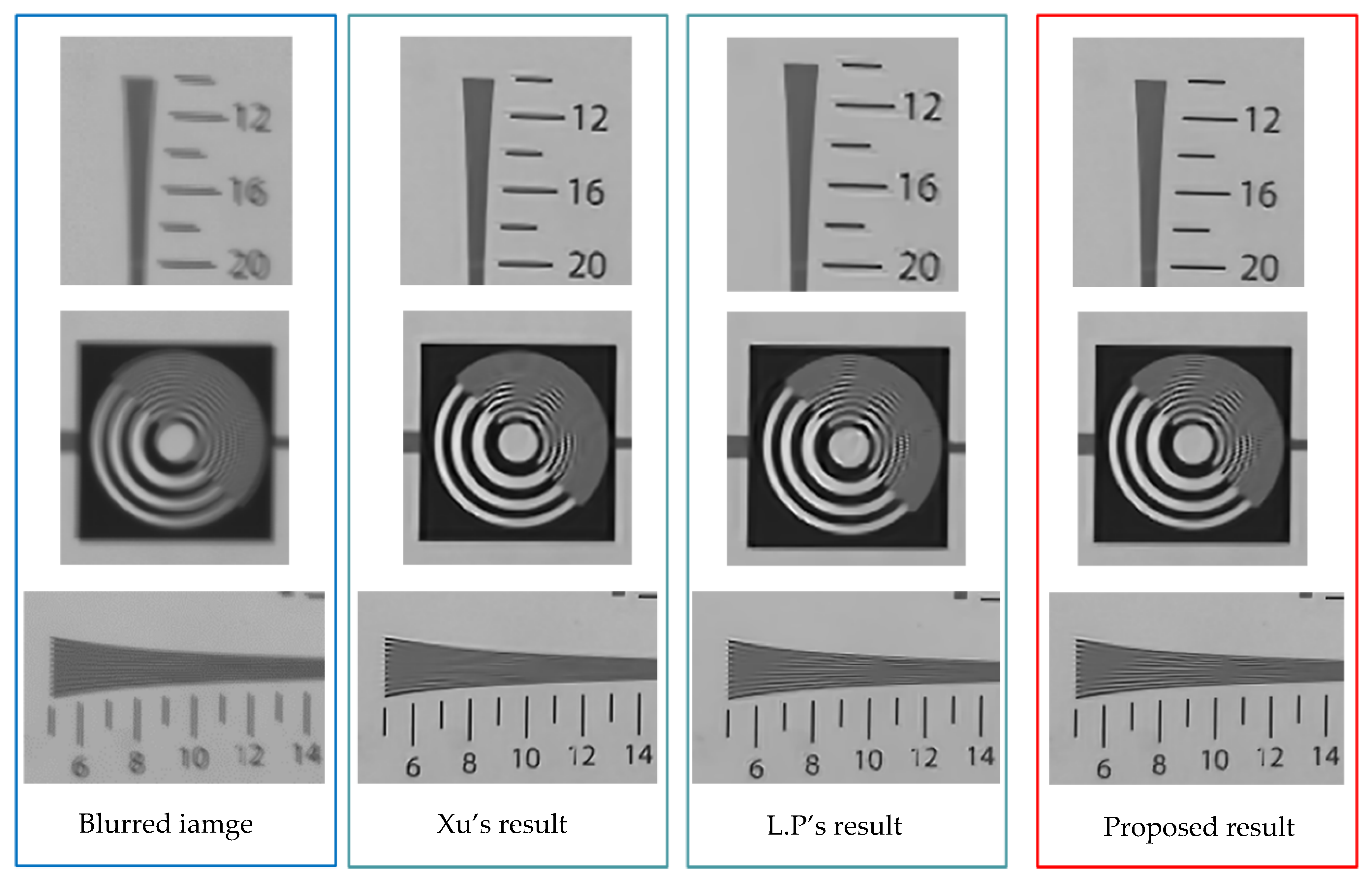
Discussion: The experimental results are shown in Figure 10 and Figure 11. First, by looking at the morphology of the blur kernels, it can be seen that the blur kernels obtained by the split block method show different blurring states, depending on the region. Therefore, if the blur kernel of the whole image is estimated according to the premise of space-invariance, it can be seen that the morphology of the kernel from the comparison methods was similar, and the results also show the main blurred motion pattern of the whole image.

However, since the blurring of the image is non-uniform, the comparison algorithms were able to obtain good results in relative regions, where the blurring patterns match well. However, a poor result was obtained in regions where the blurring patterns were widely disparate. Therefore, in Figure 12, this paper selected the parts where the blur kernel morphology differed relatively more from the comparison algorithm for comparison.

In Figure 11, in the region of the green box on the top right corner of the figure, it can be seen that the blur state estimated by the proposed method is characterized by a predominantly horizontal motion with a vertical orientation, while the morphology estimated by the comparison method is an oblique blur. This difference performance of the detail restoration was caused by the different ability of the ringing effect control in the recovery results.

Within the circular region in the lower part of the image, the corresponding blurred region is the intersection of the four blurred kernels in this method; therefore, the recovered image of this block reflects the common morphology of the four regional blurred kernels. It can be seen that an oblique motion is the main common feature of all four kernels. Thus, the results of this algorithm are only slightly better than L.P.’s in terms of ringing effects and better than those of Xu’s algorithm in terms of detail.

In the lower-left corner of the image, the blur shows a greater range of movement in the horizontal direction, according to the estimation results of this algorithm. However, the energy distribution of the blur kernels is mainly in the vertical direction. Therefore, Xu’s method has a serious loss of detail in the image, to ensure control ability of the ringing. The results of L. P’s method are not sufficient in the lateral direction. In data “6” and “8”, it shows bad ringing control in the oblique direction, and the same is shown in the location of the line cluster above.

The measurements of the indicators in Table 7 also show the higher sharpness and better restoration processed by this method.

As such, because of its split-block strategy, the proposed method is significantly more effective in dealing with blurring problems with space-variant than space-invariant algorithms.

Using the suggested software (SFR_1.41) to calculate MTF parameters. Although the MTF graph shows that each comparison algorithm has some advantages over the proposed method in some intervals, the proposed method performs better in most areas of the medium and high frequencies region. The L.P’s algorithm performs better in the region around 0.5, but lower in the region from 0.4~0.5 and 0.6~1. While the result from Xu was a little higher in the end region of 0.9~1, but lower in the region 0.3~0.9. In the MTF, the method is more stable, and the result is shaper.

6. Conclusions

In this paper, the advantages and disadvantages of the existing blind deconvolution deblur algorithms for single-channel images and multi-channel images were first analyzed, and then the characteristics of large-scale space-variant blurred images were studied. Based on synthesizing single-channel blind deconvolution and multi-channel blind deconvolution algorithms, and through theoretical derivation and experimental verification, a practical dual-channel blind deconvolution algorithm was proposed. By dividing the two-channel blurred image into blocks, the algorithm cleverly uses all the information of the image block as the correlation coefficient, takes into account the correlation of the local image and the utilization rate of the global information, and also deals with the space-variant problem of space-variant images. In the kernel estimation step, the correlation coefficient and correlation information of the dual-channel image is used to reconstruct the two iterative parts of the kernel. In the restoration part of the block image, the clustering algorithm is used to calculate the weight of the kernel, to restore and reconstruct the entire image. The final experimental results showed that the algorithm fulfilled the design expectations, and the improvement to the existing algorithm is obvious.

In the process of derivation, it was found that the algorithm still has space for further development. First, the number of methods for further enhancement can be increased. According to the derivation of [11], the more channels involved in the deblurring process, the better the restoration effect may be. A specific theoretical derivation and implementation need to be performed in the next step. Second, the block clustering restoration part of the image can also be optimized, and the weight of the corresponding pixels in the block image can be more accurately determined by introducing regularization.

References

- Fergus, R.; Singh, B.; Hertzmann, A. Removing camera shake from a single photograph. ACM 2006, 25, 787–794. [Google Scholar]
- Levin, A. Image and Depth from a Conventional Camera with a Coded Aperture. Siggraph 2007, 2007, 70-es. [Google Scholar] [CrossRef]
- Zhou, X.; Mateos, J.; Zhou, F. Variational Dirichlet Blur Kernel Estimation. IEEE Trans. Image Process. 2015, 24, 5127–5139. [Google Scholar] [CrossRef] [PubMed]
- Liu, X.; Gamal, A.E. Synthesis of high dynamic range motion blur free image from multiple captures. Circuits Syst. I Fundam. Theory Appl. IEEE Trans. 2003, 50, 530–539. [Google Scholar]
- Li, Z.; Deshpande, A.; Xin, C. Denoising vs. deblurring: HDR imaging techniques using moving cameras. In Proceedings of the 2010 IEEE Computer Society Conference on Computer Vision and Pattern Recognition, San Francisco, CA, USA, 13–18 June 2010. [Google Scholar]
- Rav-Acha, A.; Peleg, S. Two motion-blurred images are better than one. Pattern Recognit. Lett. 2005, 26, 311–317. [Google Scholar] [CrossRef]
- Yuan, L.; Sun, J.; Quan, L.; Shum, H.Y. Image deblurring with blurred noisy image pairs. In ACM SIGGRAPH 2007 Papers, Proceedings of the SIGGRAPH07: Special Interest Group on Computer Graphics and Interactive Techniques Conference, San Diego, CA, USA, 5–9 August 2007; Association for Computing Machinery: New York, NY, USA, 2007. [Google Scholar]
- Katsaggelos, A.K.; Lay, K.T.; Galatsanos, N.P. A general framework for frequency domain multi-channel signal processing. IEEE Trans. Image Process. 1993, 2, 417–420. [Google Scholar] [CrossRef] [PubMed]
- Sroubek, F.; Flusser, J. Multichannel blind deconvolution of spatially misaligned images. IEEE Trans. Image Process. 2005, 14, 874–883. [Google Scholar] [CrossRef] [PubMed] [Green Version]
- Sroubek, F.; Flusser, J.; Cristobal, G. Multiframe Blind Deconvolution Coupled with Frame Registration and Resolution Enhancement; CRC Press: Boca Raton, FL, USA, 2007. [Google Scholar]
- Sroubek, F.; Milanfar, P. Robust Multichannel Blind Deconvolution via Fast Alternating Minimization. IEEE Trans. Image Process. 2012, 21, 1687–1700. [Google Scholar] [CrossRef] [PubMed]
- Djurovi, I. BM3D filter in salt-and-pepper noise removal. EURASIP J. Image Video Process. 2016, 2016, 13. [Google Scholar] [CrossRef] [Green Version]
- Alam, M.Z.; Qian, Q.; Gunturk, B.K. Space-variant blur kernel estimation and image deblurring through kernel clustering. Signal Process. Image Commun. 2019, 76, 41–55. [Google Scholar] [CrossRef]
- Xu, Z.; Fugen, Z.; Bei, X.Z. Blind deconvolution using a nondimensional Gaussianity measure. In Proceedings of the 2014 IEEE International Conference on Image Processing, Melbourne, VIC, Australia, 15–18 September 2013. [Google Scholar]
- Harikumar, G.; Bresler, Y. Perfect Blind Restoration of Images Blurred by Multiple Filters: Theory and Efficient Algorithms. IEEE Trans. Image Process. 1999, 8, 202–219. [Google Scholar] [CrossRef] [PubMed]
- Li, X.C.; Li, H.K.; Song, B. Application of energy functional regularization model in image restoration. J. Image Graph. 2014, 19, 1247–1259. (In Chinese) [Google Scholar]
- Yang, L.; Ji, H. A Variational EM Framework With Adaptive Edge Selection for Blind Motion Deblurring. In Proceedings of the IEEE/CVF Conference on Computer Vision and Pattern Recognition (CVPR), Long Beach, CA, USA, 15–20 June 2019. [Google Scholar]
- Osher, S.; Burger, M.; Goldfarb, D.; Xu, J.; Yin, W. An iterative regularization method for total variation-based image restoration. Siam J. Multiscale Model. Simul. 2005, 4, 460–489. [Google Scholar] [CrossRef]
- Beck, A.; Teboulle, M. A Fast Iterative Shrinkage-Thresholding Algorithm for Linear Inverse Problems. Siam J. Imaging Hences 2009, 2, 183–202. [Google Scholar] [CrossRef] [Green Version]
- Boyd, S.; Parikh, N.; Chu, E.; Peleato, B.; Eckstein, J. Distributed Optimization and Statistical Learning via the Alternating Direction Method of Multipliers. Found. Trends Mach. Learn. 2010, 3, 1–122. [Google Scholar] [CrossRef]
- Wen, F.; Ying, R.; Liu, Y.; Liu, P.; Truong, T.-K. A Simple Local Minimal Intensity Prior and An Improved Algorithm for Blind Image Deblurring. IEEE Trans Circuits Syst. Video Technol. 2021, 31, 2923–2937. [Google Scholar] [CrossRef]
- Bai, Y.; Cheung, G.; Liu, X.; Gao, W. Graph-Based Blind Image Deblurring From a Single Photograph. IEEE Trans. Image Process. 2018, 28, 1404–1418. [Google Scholar] [CrossRef] [PubMed] [Green Version]
- Pan, L.; Hartley, R.; Liu, M.; Dai, Y. Phase-Only Image Based Kernel Estimation for Single Image Blind Deblurring. In Proceedings of the 2019 IEEE/CVF Conference on Computer Vision and Pattern Recognition (CVPR), Long Beach, CA, USA, 15–20 June 2019. [Google Scholar]
- ISO 122333; 2017 Photography Electronic Still Picture Imaging Resolution and Spatial Frequency Responses. ISO: Geneva, Switzerland, 2017.
- Mittal, A.; Soundararajan, R.; Bovik, A.C. Making a “Completely Blind” Image Quality Analyzer. IEEE Signal Process. Lett. 2013, 20, 209–212. [Google Scholar] [CrossRef]
Figure 1.
Structure flow chart: This figure describes the flow and components of the proposed algorithm. The input is two blurred images with different blurring patterns, but with the same object. The first step is pre-processing, which focuses on block splitting and de-noising. The second part estimates the blur kernel, block by block. The third step is the classification of the blur kernels using a clustering algorithm and the final restoration.
Figure 2.
The block layer kernel estimation flow chart. According to the EM algorithm idea, iterative kernels are estimated alternatively with the iterative image, which needs to be fixed in the iterative image when estimating the kernel and vice versa.
Figure 3.
Levin image restoration experiment. Left is PSNR and right is SSIM. This paper used the same parameters and solution methods to test the performance of the two regular terms of WG-NGM and NGM under the same conditions.
Figure 4.
The Levin library; (a) the original images from the Levin library; (b) kernels.
Figure 5.
The result; Left is the SSIM; Right is PSNR. The red line is the average. The blue box is the main area of concentration for the median 50% of the data. The black horizontal line indicates the highest value in the median region. The red cross indicates the highest value for the entire set. If there is no red cross, then the highest value is at the black horizontal line above.
Figure 9.
Result of the Kohler library. At the top, from left to right, are the results of the proposed method, Xu, and F.Wen, and the estimated kernel; below are the blurred image and details from the line above.
Figure 10.
The input blurred images and the restoration. The top line is the blurred images 1 and 2; The middle line is the results of Xu’s and L.P’s methods as space-invariant. The bottom line is the deblurred image using the proposed method as space-variant.
Figure 11.
(a) The kernels from Xu’s, L.P’s and the proposed method. The kernel results of the comparison algorithms were the results of the sample images which were processed as space-invariant images. The proposed result was obtained by processing the sample images as space-variant. Each region was estimated individually using a split block method. Based on the length and width of the image and the results of several experiments, this method chose the block size as 250 × 250 pixels, with a step size of 200 × 200 pixels. If the width or length was insufficient, edges could be added to the left and right or top and bottom edges of the image. The edges were added by duplication.; (b) MTF. The MTF measurement was measured with the edged image in the central part of the image (measured by SFR_1.41).
Figure 12.
Details of results from the green box in Figure 9: From left to right: blurred image, Xu‘s result, L.P’s result, the proposed result.