Article

Modal Decomposition of the Precessing Vortex Core in a Hydro Turbine Model

1
Kutateladze Institute of Thermophysics SB RAS, 630090 Novosibirsk, Russia
2
Physics Department, Novosibirsk State University, 630090 Novosibirsk, Russia
3
Laboratory for Flow Instabilities and Dynamics, Technische Universität Berlin, Müller-Breslau-Straße 8, 10623 Berlin, Germany
*
Author to whom correspondence should be addressed.
Submission received: 15 April 2022 / Revised: 16 May 2022 / Accepted: 17 May 2022 / Published: 19 May 2022
(This article belongs to the Special Issue Fluid Mechanics in Hydraulic Turbines)

Abstract

:
We report on the experimental study of a precessing vortex core (PVC) in an air model of a Francis turbine. The focus is placed on the modal decomposition of the PVC that occurs in the draft tube of the model turbine for a range of operation conditions. The turbulent flow fluctuations in the draft tube are assessed using stereo particle image velocimetry (PIV) measurements. Proper orthogonal decomposition (POD) is applied to the antisymmetric and symmetric components of the velocity fields to distinguish the dynamics of the azimuthal instabilities. The pressure pulsations induced by the PVC are measured by four pressure sensors mounted on the wall of the hydro turbine draft tube. Spatial Fourier decomposition is applied to the signals of the pressure sensors to identify the contributions of azimuthal modes, m = 1 and m = 2 , to the total pressure fluctuations. The analysis based on velocity and pressure data shows similar results regarding the identification of the PVC. The contribution of the m = 2 mode to the overall turbulent kinetic energy is significant for the part load regimes, where the flow rates are twice as low as at the best efficiency point (BEP). It is also shown that this mode is not the higher harmonic of the PVC, suggesting that it is driven by a different instability. Finally, we show a linear fit of the saturation amplitudes of the m = 1 and m = 2 oscillations to determine the critical bifurcation points of these modes. This yields critical swirl numbers of S c r = 0.47 and 0.61 , respectively. The fact that the PVC dynamics in hydro turbines are driven by two individual instabilities is relevant for the development of tailored active flow control of the PVC.

1. Introduction

Hydropower represents a reliable and cost-effective renewable energy source with the capacity of flexible operation over a wide range of loads that allows to meet varying energy demands. However, if the turbine operates at part-load regime, a substantial amount of swirl remains in the flow behind the runner, which produces a negative effect on the turbine operation. When the swirl intensity exceeds a critical value, the vortex core undergoes breakdown [1]. This then triggers strong hydrodynamic oscillations, which are known as the precessing vortex core (PVC) [2,3]. This phenomenon is also well known as the vortex rope, and it has been observed in many hydraulic machines from the 1950s. The PVC itself generates synchronous pressure oscillations (pressure surges) in the draft tube of the hydro turbine, which may resonate with the entire hydraulic system, causing serious damage [4,5].
Understanding the primary physical mechanisms responsible for the PVC appearance, as well as the effect of inlet flow and channel geometry, is of practical interest for further modeling and control of the PVC and was the focus of many previous studies (for detailed references, see review [6]). Nevertheless, the relationship between the velocity distributions and pressure fluctuations generated by the PVC is still not fully understood. Modern computational fluid dynamics (CFD) packages are powerful tools for the investigation of the complex three-dimensional unsteady flows in hydro turbines [7,8]. Lately, CFD has been used extensively to investigate the PVC occurrence in the draft tube of hydro turbines [9]. However, such numerical simulations require high computational resources and sufficiently long recordings to identify unsteady flow features. Moreover, there is a need for the verification of the numerical results with experimental data [10].
Experiments focusing on the PVC in large-scale hydro turbine prototypes are very expensive. An alternative approach is to carry out the experiments in laboratory-scale models [11]. Therefore, experimental studies focusing on the PVC appearance in part-load regimes are widely represented in the literature [12,13,14,15,16,17].
Another possibility is to use simplified swirl flow generators instead of the full geometrical similitude of the water passage (the spiral case, the stay vanes, the guide vanes, and the runner). Susan-Resiga et al. [18,19] have shown that laboratory-scaled vane-based swirlers designed by applying an inverse quasi-three-dimensional method can reproduce a predetermined mean velocity distribution that mimics the real inlet flow behind a hydro turbine runner. This approach has been proven as a powerful means of bringing new insights on the vortex breakdown and PVC dynamics in hydro turbines. Examples are vortex reconnection occurring at part load regimes [20,21,22,23,24] and the development of new promising methods for PVC mitigation [25,26,27,28,29]. Upon further simplifying the test rig design, the experiments may be carried out in air instead of water to investigate the PVC dynamics in more detail [30,31,32,33].
The quantitative investigations of the PVC usually require velocity measurements using non-intrusive techniques, such as laser doppler anemometry (LDA) and particle image velocimetry (PIV). Many researchers employed PIV to investigate the flow in hydraulic turbines during off-design operating conditions. The overview of different applications of PIV techniques in the context of hydro turbines can be found in [34,35]. Proper orthogonal decomposition (POD) is also used to extract the spatial structure and the energy of the PVC in the context of model hydro turbines [36,37]. To characterize the dominant frequency and amplitude of the pressure fluctuations induced by the PVC, pressure sensors installed into the draft tube cone are used [14]. Thereby, the decomposition of pressure fluctuations into asynchronous and synchronous modes are used to characterize the pressure fluctuations induced by the PVC [38].
A promising theoretical framework to analyze and control the PVC is based on global linear hydrodynamic stability analysis (LSA). Within this framework, the PVC is associated with an unstable global mode of the swirling mean flow [39,40]. LSA can be used to identify the region where the PVC is generated, and it provides deeper comprehension of flow control methods for mitigating the PVC [41,42]. To validate the results from LSA, detailed experimental information is required regarding the onset of the instability and its mode shape.
It should be noted that most experimental data available in the literature are generally limited to single operating conditions at either the part load or the BEP regimes. This study extends the previous observations and focuses on the evolution of the PVC, as the operating conditions are varied in a wide range (flow rates). This allows to track the PVC formation from deep part-load to over-load regimes (including BEP). To characterize the PVC evolution, we perform the modal decomposition of experimental data gathered in the cone of a hydro turbine model. The analysis based on velocity and pressure data shows for the first time that the PVC dynamics consist of a m = 1 single-helical part as well as a m = 2 double-helical part, where m is the azimuthal wave number. This information is quite important for developing concepts of PVC mitigation based on active flow control.
The paper is outlined as follows. In Section 2, the experimental methods are described, including the test setup, PIV and pressure fluctuation measurements. The post-processing methods are described in Section 3. The results are provided and discussed in Section 4. Finally, the main observations are summarized in Section 5.

2. Experimental Set-Up and Measurements
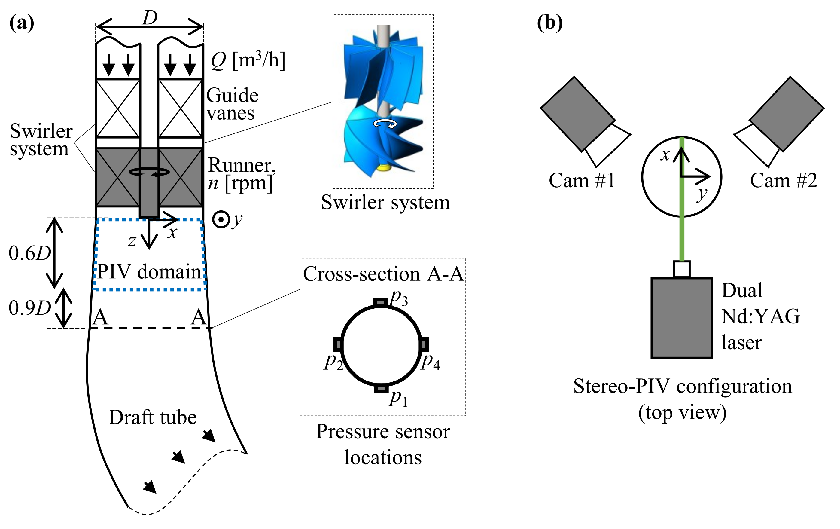
2.1. Test Section

To simplify the experimental rig and to facilitate the measurements, experiments are carried out with air as the working medium instead of water [30,43]. A detailed description of the experimental rig used in these experiments is presented in [32]. The experiments are performed, employing an open aerodynamic setup. The air flow is fed by a vortex blower, regulated and measured by a frequency converter and an ultrasonic flow meter, respectively. The runner is driven by a servo motor at a controlled rotation speed. The experimental setup includes an automated system for controlling the volumetric flow rate Q and runner speed n with uncertainties of 1.5% and 0.5%, respectively.
To mimic the velocity distribution behind the runner of a real turbine, a pair of swirlers is used: a stationary swirler as guide vanes and a rotary swirler as the runner (swirler system is shown in the Figure 1a). The pair of swirlers is designed for the optimal operating conditions (the best efficiency point—BEP) corresponding to a volumetric flow rate of Q c = 174.6 m 3 /h and a runner speed of n c = 40.53 Hz [31].
The test section consists of a pair of swirlers and a scaled-down laboratory model of the Francis-99 draft tube (from [44]) with an inlet diameter of D = 100 mm (Figure 1a). The region of interest is located at the cone of the draft tube, where vortex breakdown occurs. To gain optical access, the cone part of the Francis-99 draft tube is made out of glass. The PIV domain and pressure sensor arrangement are shown in Figure 1a. The origin of the used Cartesian coordinate system is set to the outlet plane on the central axis (Figure 1a,b). The z-coordinate coincides with the axial direction (from top to bottom), which is the main flow direction. The x-coordinate is radially directed from the turbine axis, and the y-coordinate is normal to the PIV measurement plane, respectively. The facility is operated at flow rates within the range between 0.3 Q c and 1.5 Q c at a constant runner speed of n c .

2.2. Wall Pressure Measurements

The pressure fluctuations are recorded by four microphones (Behringer ECM 8000, Willich, Germany), which are arranged circumferentially at cross section A-A (Figure 1a). The signals from the sensors are recorded for 900 s at a sampling frequency of 20 kHz. As the typical PVC frequency is at around 17 Hz, these acquisition parameters ensure sufficient resolution.

2.3. Stereo-PIV Measurements

Figure 1b shows the used stereo-PIV configuration. A double-head Nd:YAG laser (Quantel, EverGreen, Lannion, France) illuminates the tracer particles. The laser beam is converted into a laser sheet with a thickness of less than 1 mm by using a system of cylindrical and spherical lenses. On average, the pulse energy is 70 mJ before the laser sheet optics (measured by a power meter Coherent LabMax). Particle images are captured by a pair of CCD cameras (Bobcat ImperX, Boca Raton, FL, USA). The PIV images (4904 × 3280 pixels in size) are processed by using an in-house software ActualFlow. A Laskin nozzle generator is used to seed the flow with oil droplets. The time separation between two PIV laser pulses is 30 μ s. The images are preprocessed to remove the background (minimal intensity for each pixel). During four iterations of an adaptive cross-correlation algorithm, the interrogation area is reduced from 64 × 64 to 16 × 16 pixels. The spatial overlap rate between the interrogation areas is 50%, and the resulting spatial resolution is 0.5 mm. For each operating regime, a set of 1500 snapshots is acquired.

3. Post-Processing Routines

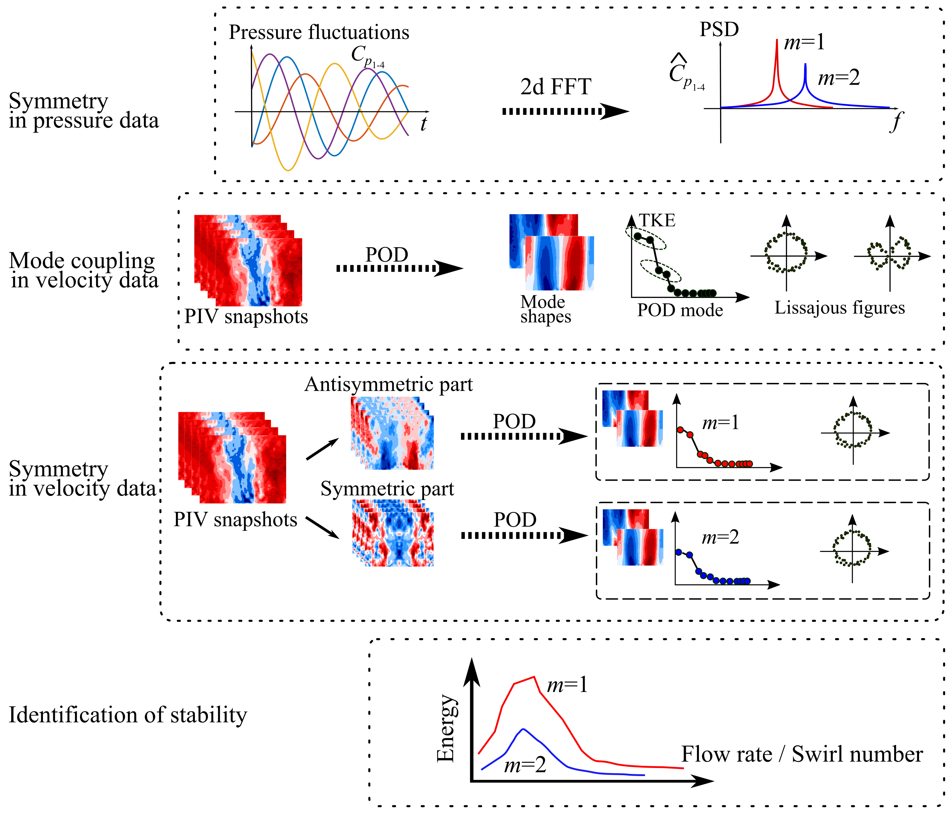
3.1. Spatial Fourier Mode Decomposition

The pressure signals are used to characterize the amplitude and frequency of the PVC in the draft tube cone. In the following, the pressure fluctuations are non-dimensionalized by defining the pressure coefficient C p as
C p j = p j V 0 2 ,
where p j is the discrete pressure signal obtained from one microphone, and V 0 = 4 Q / π D 2 is the bulk velocity in the considered section.
The pressure coefficients C p j obtained from four microphones are decomposed into spatial (azimuthal) and temporal Fourier modes. A similar decomposition is applied in the paper of [45] to calculate the contribution of the PVC to the pressure pulsations in a swirl flame. Accordingly, the 2D Discrete Fourier transform reads
C ^ p f , m = 1 N j N k j = 0 N j 1 k = 0 N k 1 e 2 π i ( f N j j + m N k k ) C p j + 1 , k + 1
where C p j , k is a matrix of pressure coefficients of the k-th sensors and j is the index of the recorded discrete time intervals ( N j is a length of the time series). With four microphones arranged in a circumferential direction ( N k = 4), azimuthal modes with wave numbers m = 0, −1, 1, ±2 can be identified. The matrix C ^ p f , m contains the complex-valued Fourier coefficients at frequency f and azimuthal mode m.
To analyze the spectrum of the flow dynamics, we use the Welch’s overlapped segment averaging spectral estimation with a segment length of 2 18 sampling points and an overlap of 50%. The power spectral density (PSD) of C ^ p f , m is generated for different operating regimes by varying the parameter Q / Q c . To allow relative comparisons, all values are normalized with respect to an overall maximum value. The frequencies are normalized with respect to the runner speed n c .
Referring to previous studies [1,39,46], the PVC dynamics are characterized by a co-rotating counter winding mode. In our nomenclature, this refers to modes with positive azimuthal wave numbers m and positive frequency. In this regard, we focus our analysis on the spectra of the m = 1 and m = 2 modes only. It should be noted that pressure fluctuations of wave number m = 0 are not considered in the study, as it is quite difficult to separate the hydrodynamic-induced pressure pulsations from the planar acoustic noise that is present in the experimental rig.

3.2. Proper Orthogonal Decomposition (POD)

To extract energy-ranked coherent structures in the swirl flow inside the draft tube cone, we employ classic proper orthogonal decomposition (POD) [47]. This method has been used extensively to identify coherent structures in various flow applications. In this work, POD is used as an alternative to the classic conditional-phase averaging operation [48].
The POD is based on the following decomposition
V ( x , t ) = V ¯ ( x ) + V ( x , t ) = V ¯ ( x ) + i = 1 N a i ( t ) ϕ i ( x ) ,
where the fluctuating part is decomposed into a sum of spatial modes ϕ i and corresponding temporal coefficients a i . This basis is built based on the spatial correlation among the individual velocity snapshots, yielding a correlation matrix. The temporal coefficients a i are derived from the eigenvectors of the correlation matrix and describe the dynamics of the corresponding mode ϕ i . The spatial modes are obtained from a projection of the snapshots onto the temporal coefficients. More details on POD are given in [39,49,50].

3.3. Symmetric and Antisymmetric Decomposition of the Velocity Fields

In this study, we decompose the velocity fluctuations into symmetric and antisymmetric components with respect to the z-axis [51]:
V = V s y m + V a s y m ,
where the symmetric part is defined as
V x s y m ( x , y , z ) = ( V x ( x , y , z ) V x ( x , y , z ) ) / 2 , V y s y m ( x , y , z ) = ( V y ( x , y , z ) + V y ( x , y , z ) ) / 2 , V z s y m ( x , y , z ) = ( V z ( x , y , z ) + V z ( x , y , z ) ) / 2 ,
and the antisymmetric one is defined as
V x a s y m ( x , y , z ) = ( V x ( x , y , z ) + V x ( x , y , z ) ) / 2 , V y a s y m ( x , y , z ) = ( V y ( x , y , z ) V y ( x , y , z ) ) / 2 , V z a s y m ( x , y , z ) = ( V z ( x , y , z ) V z ( x , y , z ) ) / 2 .
The POD is then applied to each of the resulting velocity fields separately. This allows to enforce the symmetry properties for each POD mode.
The decomposition of the velocity field (and POD modes) into a symmetric and antisymmetric part allows separating the coherent structures between even and odd azimuthal wave numbers. The aim is to use this approach to separate the coherent structures into azimuthal modes m = 1 and m = 2 , as detected by the pressure sensors, and to evaluate their interplay.

3.4. Outline of Applied Methods

The analysis of the pressure fluctuations and PIV data is carried out according to the flowchart displayed in Figure 2. In detail, the following steps are taken:
-
Extract symmetry properties from the four signals of pressure fluctuations by using the spatial Fourier mode decomposition;
-
Find a mode coupling in the velocity data by classical POD analysis;
-
Extract symmetry properties from POD of the symmetric/antisymmetric decomposed velocity data;
-
Track modes as a function of operating condition and identify the onset of instabilities.

4. Results and Discussion

4.1. Wall Pressure Fluctuations

To identify the PVC, we consider the spectra of pressure fluctuations as a function of operating condition Q / Q c , shown in Figure 3. The pressure fluctuations in terms of the semi-log PSD plots of | C ^ p f , m | are analyzed for azimuthal wave numbers m = 1 and m = 2 . The highest amplitude of the pressure fluctuations is registered for the flow rate of 0.5 Q c , as was previously reported in [32]. Therefore, this value is used for the spectra normalization. The spectral contents of the modes m = 1 and m = 2 are relatively sharp with a clear peak at the frequency below than that of the runner n c . In addition, a relatively small peak at the frequency of the runner speed n c can be noticed at both spectra. Hence, the spectra show that two oscillatory modes present in the pressure fluctuations for a wide range of part load regimes.
For the azimuthal wave number m = 1 , there is a dominant peak in the frequency range between 0.4 and 0.45 n c . Starting from 0.4 Q c , this peak increases with the flow rate, reaching a maximum amplitude at 0.5 Q c , and then decreasing and completely disappearing at 0.8 Q c . It is considered to be induced by the PVC.
For the mode m = 2 , there are also similar peaks at this frequency, but there are also peaks at double frequency. The occurrence of m = 2 peaks at the double frequency of the m = 1 is indicative of a strong higher harmonic. However, the relative energy content is too high for this to be the case. Moreover, the existence of m = 2 fluctuations at the m = 1 frequency indicates a substantial energy back-scatter from the dominant m = 2 to the m = 1 frequency. These observations apparently suggest that the m = 2 mode is not simply a higher harmonic of the m = 1 , but driven by another instability.

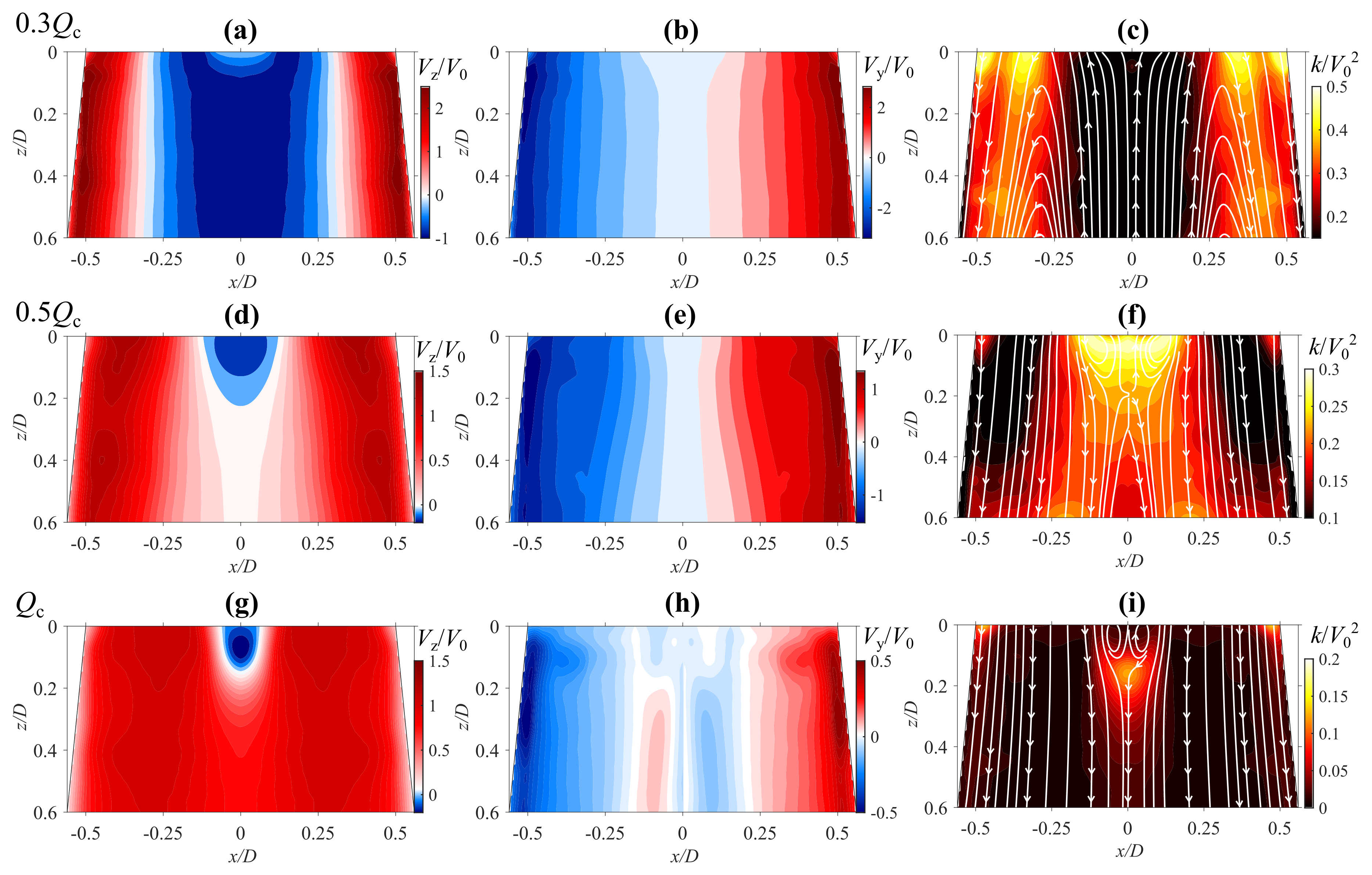
4.2. Mean Velocity Distributions

Next, we address the change of the time-averaged flow characteristics for different operating conditions. Figure 4 shows the distributions of the axial and tangential components of the mean velocity and turbulent kinetic energy (TKE), k = ( V x 2 + V y 2 + V z 2 ) / 2 for three different flow rates. The flow rate of 0.3 Q c corresponds to the deep part load regime with the highest swirl and with the low level and broad pressure fluctuations of m = 1 . The flow rate of 0.5 Q c corresponds to the part load regime with the highest pressure fluctuations amplitude for m = 1 . The regime with flow rate close to Q c is considered the optimal regime of the BEP.
In the case of the deep part load regime at flow rate 0.3 Q c , there is a large central recirculation zone (CRZ) behind the swirler centerbody. This flow is also characterized by high turbulent fluctuations, with a TKE level of up to 50% of the bulk flow velocity. It is noteworthy that the fluctuation level inside the recirculation zone is rather weak. The mean flow at the part load ( Q = 0.5 Q c ) is characterized by a smaller CRZ with intensive velocity fluctuations inside. The CRZ is followed by a wake, where the velocity fluctuations are also strong. For the BEP case ( Q = Q c ), there is a small CRZ behind the bluff body. The flow is characterized by a local maximum of the TKE downstream of the CRZ without a large turbulent wake. It is noteworthy that there is a region of flow reversal in this case, with two concentric counter-rotating cylindrical rod-like swirling flows. This observation has already been discussed in [32].

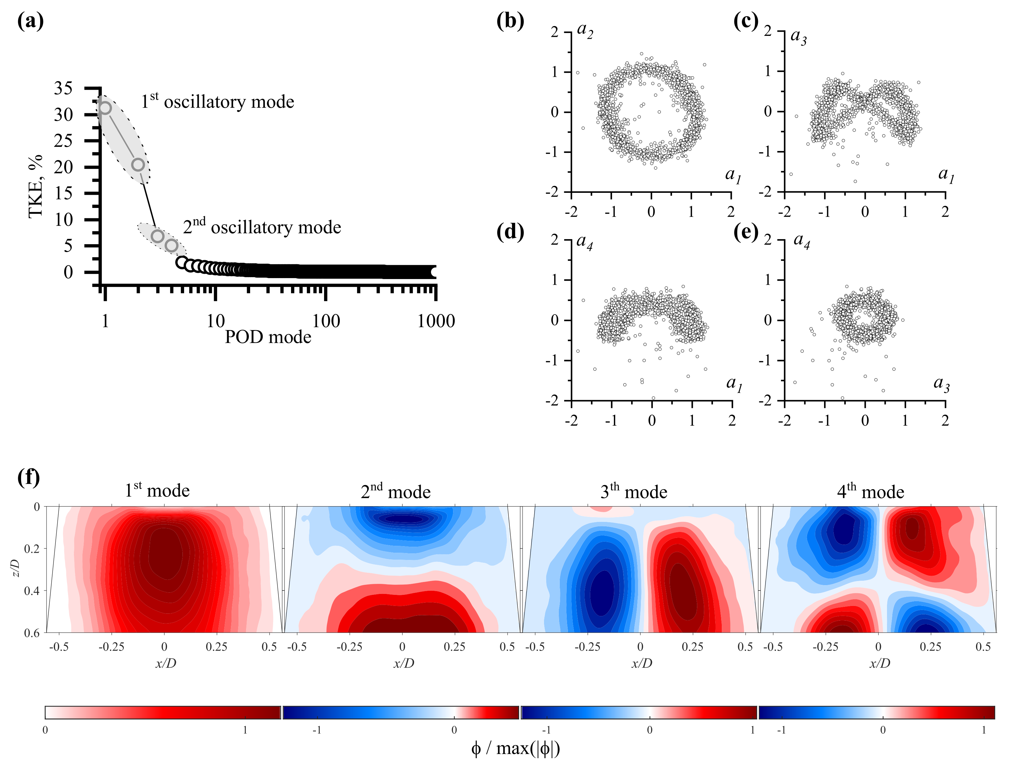
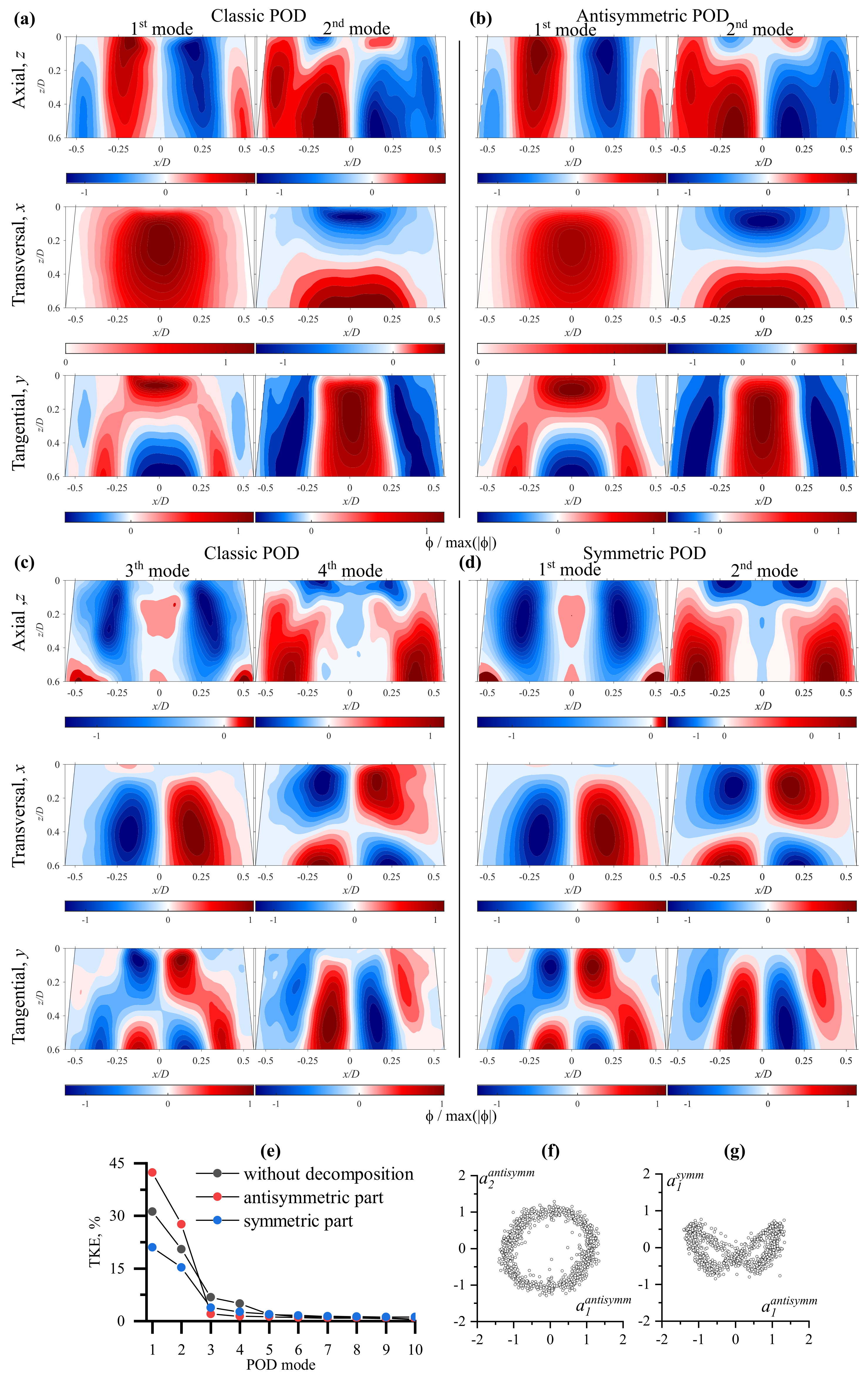
4.3. Classic POD at Part-Load Regime

We now focus on the modal decomposition of the velocity fluctuations to understand the influence of the PVC for the case of the highest level of pressure fluctuations (flow rate of 0.5 Q c ). For this purpose, the classical POD, as described in Section 3.2, is applied to the recorded PIV snapshot sequence. The eigenvalue spectrum of the POD modes is shown in Figure 5a. The POD spectrum shows that the first two leading modes contain 52% of the total TKE, while the second two modes contain approximately 12%. The energy contained in the first two modes is expected to be associated with the unsteady dynamics of the PVC, as was previously observed in other swirling flows [39,52].
To elucidate the temporal correlation of the identified coherent structures in the first four POD modes, the phase portraits of the corresponding temporal amplitudes a i are investigated (Figure 5b–e). Considering the phase portrait of a 1 and a 2 (Figure 5b), it is clearly seen that the modes have a π / 2 phase shift and describe a quasi-periodic process [39]. The comparison of the values of a 1 ( a 3 ) and a 1 ( a 4 ) reveals that the second pair of modes is synchronized with the first pair and oscillates at the double frequency, as indicated by the shape of the Lissajous figure (Figure 5c,d). In addition, modes a 3 and a 4 have a π / 2 phase shift between each other and describe an oscillatory process too. This analysis clearly shows that the flow dynamics are dominated by four temporarily synchronized modes. The first and second pairs of the POD modes combine to two individual oscillatory motions that are synchronized, where the first rotates at half the frequency of the second.
The shape of the leading four POD modes are shown in Figure 5f for the transversal velocity component (x-component). All values are normalized with respect to the maximum value. The first two POD modes look typical for the PVC possessing a symmetrical distribution with respect to the z-axis [39,51]. The next two mode shapes (3rd and 4th) have an antisymmetric distribution. Generally, this fact corresponds to even/odd azimuthal wave numbers. While the first two modes most likely represent a m = 1 mode, the next two modes (3rd and 4th) represent a m = 2 mode, considering the symmetry properties of the mode shapes. It is also evident that the antisymmetric mode pair has a non-vanishing radial velocity component on the jet axis ( x / D = 0 ). According to [51,53], only a mode with an azimuthal wave number m = 1 can have this property. Moreover, it is most likely that the 3rd and 4th POD modes correspond to an azimuthal mode m = 2 , as it has the double frequency of the m = 1 mode (see Lissajous figures on Figure 5c,d). From the pressure spectra, we also know of the existence of the m = 2 mode at double the frequency of the m = 1 mode for this operating regime (Figure 3, 0.5 Q c ).

4.4. Symmetric/Antisymmetric POD at Various Flow Regimes

According to the decomposed pressure fluctuations in Figure 3, the mode m = 2 has a higher amplitude than is expected for the first harmonic of the PVC. This indicates that the m = 2 mode is driven by an individual mechanism. To shed more light on this, we intend to track the m = 1 and m = 2 instabilities as a function of the operating condition. For this purpose, we apply a modified POD to the symmetric/antisymmetric decomposed velocity fluctuations, which allows for a clear separation, even at conditions where the modes are relatively weak.
To extract the antisymmetric and symmetric POD structures, the recorded PIV snapshot sequence is decomposed into antisymmetric and symmetric parts, according to Equation (6). The resulting spatial modes are shown in Figure 6a–d and compared to the classic POD. It is clearly seen that the first mode pair of the classical POD is equivalent to the first mode pair of the antisymmetric POD. Considering Figure 6c,d, it is shown that the second mode pair of the classical POD decomposition (3rd and 4th) is equivalent to the first mode pair of the symmetrical POD. The relative energy content of the POD modes computed from the antisymmetric and symmetric parts of the velocity fluctuations likewise feature a gap between the first mode pair and the remaining modes (Figure 6e). Additionally, the phase portrait of the first two modes in Figure 6f indicates an oscillatory motion. The phase portrait of Figure 6g indicates a synchronization between a 1 a n t i s y m m and a 1 s y m m . The fact that m = 2 is double the frequency of m = 1 is also proven by the eight-like shape of the Lissajous figure (Figure 6g). All these observations suggest that the first and second antisymmetric modes represent the global mode m = 1 and can be associated with the PVC. In turn, the first and second symmetric modes represent the mode m = 2 .
Thus, the POD analysis based on the decomposed velocity snapshots allows distinguishing between modes with azimuthal wave numbers m = 1 and m = 2 by consideration of the antisymmetric and symmetric parts of the velocity fluctuations, respectively. This is particularly important when considering flow regimes where vortex dynamics are less dominant and covered by turbulent noise. In this case, classical POD will not well be able to clearly distinguish between m = 1 and m = 2 due to the mixing of the modes.

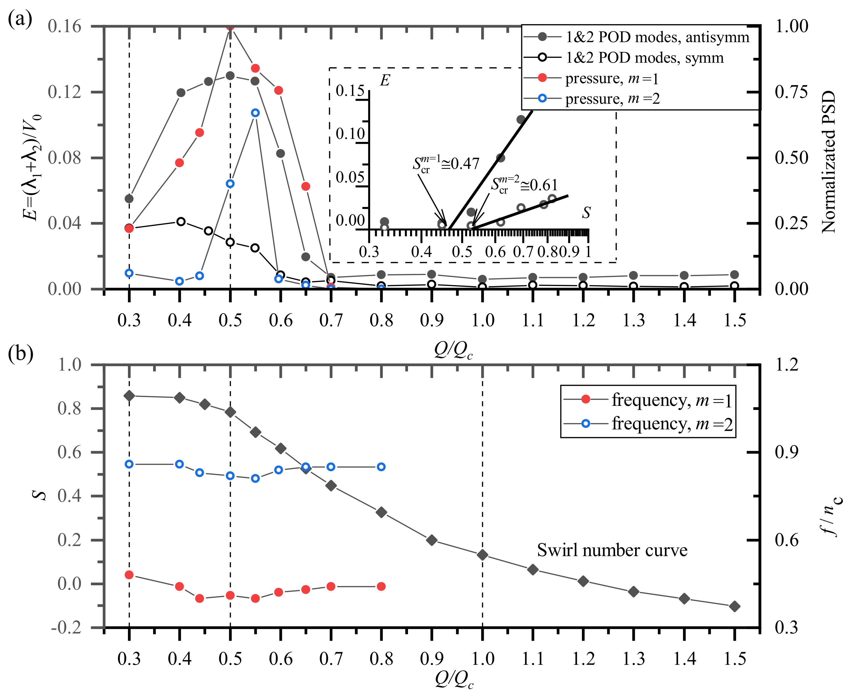
4.5. Identification of Stability

In the final step, we apply the decomposed POD approach to the PIV data acquired at a range of flow rates to track the onset of the m = 1 and m = 2 instability. Figure 7a summarizes the results. The left ordinate axis represents the energy content of the leading mode pair in terms of E = ( λ 1 + λ 2 ) / V 0 2 calculated from the antisymmetric ( m = 1 ) and symmetric ( m = 2 ) parts of the velocity fluctuations. The right ordinate axis represents the level of the dominant peak of the PSD spectra of the pressure data (refer to Figure 3). The abscissa axis represents the flow rate, with Q / Q c = representing the BEP.
Comparing the results from the POD and PSD, we observe a similar qualitative trend for the m = 1 mode. For the m = 2 mode, we observe quite a few deviations. The differences are most likely due to the different spatial locations of the PIV domain and cross section A (Figure 1a), where the acoustic sensors are mounted. Further, the difference is also due to the fact that we compare kinetic energy and pressure, which are two different quantities. The impact of mode m = 2 on the energy content is significant for both cases in the part load regime (between 0.5 Q c and 0.55 Q c ). It again shows that with the contribution of m = 2 the energy content should not be considered as a higher harmonic of PVC.
The evaluated swirl number of the flows is plotted in Figure 7b as a function of Q. The swirl number is calculated based on the mean velocity distributions, as given in Appendix A. In addition, the normalized frequencies of the fluctuations of the m = 1 and m = 2 modes are shown as a function of Q / Q c (right axis). The frequencies remain rather constant with the changing flow rate, with a slight minimum at the point of maximal registered pressure fluctuations (0.5 Q c ). It is further seen that the frequency of m = 2 is approximately twice the frequency of m = 1 .
Finally, we would like to evaluate if the m = 1 and m = 2 modes originate from two individual stability mechanisms. According to [1,54], the observed single-helical PVC is the result of a self-excited global mode due to a supercritical Hopf bifurcation. Close to the bifurcation point, the limit-cycle amplitude of such a mode is well represented by the Landau equation, which implies that with the swirl number as the control parameter, the limit-cycle amplitude is proportional to S S c r . Upon consideration of E = ( λ 1 + λ 2 ) / V 0 2 as the squared saturation amplitude, we should expect this quantity to linearly depend on the swirl number for the supercritical Hopf bifurcation type.
The zoomed insert of Figure 7a shows the energy of the leading POD mode pair of the m = 1 and m = 2 modes as a function of the swirl number. The linear dependence is clearly seen. A linear fit of the saturation amplitudes further yields a critical swirl number of S c r m = 1 = 0.47 and, S c r m = 2 = 0.61 , for the two modes, respectively. The linear dependence we observe in this figure, as well as the two different bifurcation points, clearly show that the two modes correspond to two individual global instabilities.

5. Conclusions

The swirling air flow of the hydro turbine model is studied using stereo-PIV and four wall-pressure sensors. The facility allows investigating the flow dynamics for flow rates ranging from the best efficiency point (BEP) to deep part load. The focus of the study is on the modal decomposition of the precessing vortex core (PVC) that arises at part load conditions.
Spatial Fourier decomposition is applied to the signals from the pressure sensors to identify the contributions of the azimuthal wave numbers m = 1 and m = 2 to the total level of pressure fluctuations. The proper orthogonal decomposition (POD) is applied to the antisymmetric and symmetric velocity fluctuations to extract the mode shape corresponding to the modes m = 1 and m = 2 .
Both the velocity and pressure data show a similar range where the PVC is present. The m = 2 oscillations are synchronized to the m = 1 mode and oscillate at double the frequency. However, the energy content is quite significant in the part load regime and comparable to the one of the m = 1 mode. This suggests that the m = 2 mode is not a higher harmonic of the m = 1 mode, but driven by the own instability mechanisms.
To further investigate the onset of the two instability modes, we observe their saturation amplitudes as a function of the swirl number. From the fit of the Landau amplitude equation, we identify two critical swirl numbers of S c r = 0.47 and 0.61 for m = 1 and m = 2 , respectively.
The identification of two individual modes, which could easily be mistaken as higher harmonics, is important to develop new concepts of active flow control, e.g., energy-efficient excitation of defined azimuthal modes ( m = 1 and m = 2 ) may be more effective than other known control methods of the PVC.

Author Contributions

Conceptualization, I.L., K.O. and V.D.; methodology, I.L., K.O., V.D. and S.S.; experimentation I.L., D.S. and E.G.; writing—original draft preparation, I.L.; writing—review and editing, K.O., V.D. and S.S.; supervision, S.A. All authors have read and agreed to the published version of the manuscript.

Funding

This investigation was supported by the Russian Foundation for Basic Research (grant number 20-58-12012, in the part of PIV measurements). The design and installation of the experimental setup was carried out partly within the framework of a state contract with IT SB RAS. The funding of the German Research Foundation (grant number 429772199) is acknowledged.

Conflicts of Interest

The authors declare no conflict of interest.

Appendix A. Swirl Number Definition

Swirl number can be determined from the measured mean velocity distributions ( V z is the axial component and V y is the tangential component):
S = 2 0 D / 2 V z ( x ) V y ( x ) x 2 d x D 0 D / 2 V z ( x ) 2 x d x ,
where the integration is performed at axial position z = 0. Integration limits are x = 0 and x = D / 2 , where D is the inlet diameter of the cone.

References

  1. Liang, H.; Maxworthy, T. An experimental investigation of swirling jets. J. Fluid Mech. 2005, 525, 115–159. [Google Scholar] [CrossRef]
  2. Gupta, K.; Lilley, D.; Syred, N. Swirl Flows; Abacus Press: Kent, UK, 1984. [Google Scholar]
  3. Syred, N. A review of oscillation mechanisms and the role of the precessing vortex core (PVC) in swirl combustion systems. Prog. Energy Combust. Sci. 2006, 32, 93–161. [Google Scholar] [CrossRef]
  4. Dörfler, P.; Sick, M.; Coutu, A. Flow-Induced Pulsation and Vibration in Hydroelectric Machinery: Engineer’s Guidebook for Planning, Design and Troubleshooting; Springer Science & Business Media: Berlin/Heidelberg, Germany, 2012. [Google Scholar]
  5. Favrel, A.; Gomes Pereira Junior, J.; Müller, A.; Landry, C.; Yamamoto, K.; Avellan, F. Swirl number based transposition of flow-induced mechanical stresses from reduced scale to full-size Francis turbine runners. J. Fluids Struct. 2020, 94, 102956. [Google Scholar] [CrossRef]
  6. Kumar, S.; Cervantes, M.J.; Gandhi, B.K. Rotating vortex rope formation and mitigation in draft tube of hydro turbines—A review from experimental perspective. Renew. Sustain. Energy Rev. 2021, 136, 110354. [Google Scholar] [CrossRef]
  7. Trivedi, C.; Cervantes, M.J.; Gunnar Dahlhaug, O. Numerical techniques applied to hydraulic turbines: A perspective review. Appl. Mech. Rev. 2016, 68, 010802. [Google Scholar] [CrossRef]
  8. Tiwari, G.; Kumar, J.; Prasad, V.; Patel, V.K. Utility of CFD in the design and performance analysis of hydraulic turbines—A review. Energy Rep. 2020, 6, 2410–2429. [Google Scholar] [CrossRef]
  9. Goyal, R.; Gandhi, B.K. Review of hydrodynamics instabilities in Francis turbine during off-design and transient operations. Renew. Energy 2018, 116, 697–709. [Google Scholar] [CrossRef]
  10. Trivedi, C.; Dahlhaug, O.G. A comprehensive review of verification and validation techniques applied to hydraulic turbines. Int. J. Fluid Mach. Syst. 2019, 12, 345–367. [Google Scholar] [CrossRef]
  11. Valentín, D.; Presas, A.; Valero, C.; Egusquiza, M.; Egusquiza, E.; Gomes, J.; Avellan, F. Transposition of the mechanical behavior from model to prototype of Francis turbines. Renew. Energy 2020, 152, 1011–1023. [Google Scholar] [CrossRef]
  12. Ciocan, G.D.; Iliescu, M.S.; Vu, T.C.; Nennemann, B.; Avellan, F. Experimental Study and Numerical Simulation of the FLINDT Draft Tube Rotating Vortex. J. Fluids Eng. 2007, 129, 146–158. [Google Scholar] [CrossRef]
  13. Kirschner, O.; Ruprecht, A.; Göde, E.; Riedelbauch, S. Experimental investigation of pressure fluctuations caused by a vortex rope in a draft tube. Proc. IOP Conf. Ser. Earth Environ. Sci. 2012, 15, 062059. [Google Scholar] [CrossRef]
  14. Trivedi, C.; Cervantes, M.J.; Gandhi, B.K.; Dahlhaug, O.G. Experimental and numerical studies for a high head Francis turbine at several operating points. J. Fluids Eng. 2013, 135, 111102. [Google Scholar] [CrossRef]
  15. Favrel, A.; Müller, A.; Landry, C.; Yamamoto, K.; Avellan, F. Study of the vortex-induced pressure excitation source in a Francis turbine draft tube by particle image velocimetry. Exp. Fluids 2015, 56, 1–15. [Google Scholar] [CrossRef]
  16. Favrel, A.; Müller, A.; Landry, C.; Yamamoto, K.; Avellan, F. LDV survey of cavitation and resonance effect on the precessing vortex rope dynamics in the draft tube of Francis turbines. Exp. Fluids 2016, 57, 1–16. [Google Scholar] [CrossRef]
  17. Favrel, A.; Gomes Pereira Junior, J.; Landry, C.; Müller, A.; Nicolet, C.; Avellan, F. New insight in Francis turbine cavitation vortex rope: Role of the runner outlet flow swirl number. J. Hydraul. Res. 2018, 56, 367–379. [Google Scholar] [CrossRef]
  18. Susan-Resiga, R.; Muntean, S.; Bosioc, A. Blade design for swirling flow generator. In Proceedings of the 4th German–Romanian Workshop on Turbomachinery Hydrodynamics (GRoWTH), Stuttgart, Germany, 12–15 June 2008. [Google Scholar]
  19. Muntean, S.; Bosioc, A.; Stanciu, R.; Tanasa, C.; Susan-Resiga, R.; Vekas, L. 3D numerical analysis of a swirling flow generator. In Proceedings of the 4th IAHR International Meeting of the Workgroup on Cavitation and Dynamic Problems in Hydraulic Machinery and Systems, Belgrade, Serbia, 26–28 October 2011; pp. 115–125. [Google Scholar]
  20. Alekseenko, S.V.; Kuibin, P.A.; Shtork, S.I.; Skripkin, S.G.; Tsoy, M.A. Vortex reconnection in a swirling flow. JETP Lett. 2016, 103, 455–459. [Google Scholar] [CrossRef]
  21. Skripkin, S.; Tsoy, M.; Shtork, S.; Hanjalić, K. Comparative analysis of twin vortex ropes in laboratory models of two hydro-turbine draft-tubes. J. Hydraul. Res. 2016, 54, 450–460. [Google Scholar] [CrossRef]
  22. Skripkin, S.G.; Tsoy, M.A.; Kuibin, P.A.; Shtork, S.I. Study of Pressure Shock Caused by a Vortex Ring Separated From a Vortex Rope in a Draft Tube Model. J. Fluids Eng. 2017, 139. [Google Scholar] [CrossRef]
  23. Štefan, D.; Rudolf, P.; Hudec, M.; Uruba, V.; Procházka, P.; Urban, O. Experimental investigation of vortex ring formation as a consequence of spiral vortex re-connection. Proc. IOP Conf. Ser. Earth Environ. Sci. 2019, 405, 012033. [Google Scholar] [CrossRef] [Green Version]
  24. Sentyabov, A.; Platonov, D.; Minakov, A.; Lobasov, A. Numerical study of the vortex breakdown and vortex reconnection in the flow path of high-pressure water turbine. Proc. J. Phys. Conf. Ser. 2021, 2088, 012040. [Google Scholar] [CrossRef]
  25. Tǎnasǎ, C.; Bosioc, A.I.; Susan-Resiga, R.F.; Muntean, S. Experimental investigations of the swirling flow in the conical diffuser using flow-feedback control technique with additional energy source. Proc. IOP Conf. Ser. Earth Environ. Sci. 2012, 15, 062043. [Google Scholar] [CrossRef]
  26. Bosioc, A.I.; Susan-Resiga, R.; Muntean, S.; Tanasa, C. Unsteady pressure analysis of a swirling flow with vortex rope and axial water injection in a discharge cone. J. Fluids Eng. 2012, 134, 081104. [Google Scholar] [CrossRef]
  27. Tănasă, C.; Muntean, S.; Bosioc, A.I.; Susan-Resiga, R.; Ciocan, T. Influence of the air admission on the unsteady pressure field in a decelerated swirling flow. UPB Sci. Bull. Ser. D 2016, 78, 161–170. [Google Scholar]
  28. Tănasă, C.; Bosioc, A.; Muntean, S.; Susan-Resiga, R. A novel passive method to control the swirling flow with vortex rope from the conical diffuser of hydraulic turbines with fixed blades. Appl. Sci. 2019, 9, 4910. [Google Scholar] [CrossRef] [Green Version]
  29. Bosioc, A.I.; Tănasă, C. Experimental study of swirling flow from conical diffusers using the water jet control method. Renew. Energy 2020, 152, 385–398. [Google Scholar] [CrossRef]
  30. Cassidy, J.J. Experimental Study and Analysis of Draft-Tube Surging; BUR Reclam REP HYD-591; Bureau of Reclamation: Denver, CO, USA, 1969; p. 31. [Google Scholar]
  31. Sonin, V.; Ustimenko, A.; Kuibin, P.; Litvinov, I.; Shtork, S. Study of the velocity distribution influence upon the pressure pulsations in draft tube model of hydro-turbine. Proc. IOP Conf. Ser. Earth Environ. Sci. 2016, 49, 82020. [Google Scholar] [CrossRef]
  32. Litvinov, I.; Shtork, S.; Gorelikov, E.; Mitryakov, A.; Hanjalic, K. Unsteady regimes and pressure pulsations in draft tube of a model hydro turbine in a range of off-design conditions. Exp. Therm. Fluid Sci. 2018, 91, 410–422. [Google Scholar] [CrossRef]
  33. Liu, Z.; Favrel, A.; Miyagawa, K. Effect of the conical diffuser angle on the confined swirling flow induced Precessing Vortex Core. Int. J. Heat Fluid Flow 2022, 95, 108968. [Google Scholar] [CrossRef]
  34. Nobach, H. Limits in Planar PIV Due to Individual Variations of Particle Image Intensities; OCLC: 884225910; INTECH Open Access Publisher: London, UK, 2012. [Google Scholar]
  35. Goyal, R.; Gandhi, B.; Cervantes, M.J. PIV measurements in Francis turbine—A review and application to transient operations. Renew. Sustain. Energy Rev. 2018, 81, 2976–2991. [Google Scholar] [CrossRef]
  36. Štefan, D.; Hudec, M.; Uruba, V.; Procházka, P.; Urban, O.; Rudolf, P. Experimental investigation of swirl number influence on spiral vortex structure dynamics. IOP Conf. Ser. Earth Environ. Sci. 2021, 774, 012085. [Google Scholar] [CrossRef]
  37. Kumar, S.; Khullar, S.; Cervantes, M.J.; Gandhi, B.K. Proper orthogonal decomposition of turbulent swirling flow of a draft tube at part load. IOP Conf. Ser. Earth Environ. Sci. 2021, 774, 012091. [Google Scholar] [CrossRef]
  38. Goyal, R.; Cervantes, M.J.; Gandhi, B.K. Characteristics of Synchronous and Asynchronous modes of fluctuations in Francis turbine draft tube during load variation. Int. J. Fluid Mach. Syst. 2017, 10, 164–175. [Google Scholar] [CrossRef]
  39. Oberleithner, K.; Sieber, M.; Nayeri, C.N.; Paschereit, C.O.; Petz, C.; Hege, H.C.; Noack, B.R.; Wygnanski, I. Three-dimensional coherent structures in a swirling jet undergoing vortex breakdown: Stability analysis and empirical mode construction. J. Fluid Mech. 2011, 679, 383–414. [Google Scholar] [CrossRef] [Green Version]
  40. Pasche, S.; Avellan, F.; Gallaire, F. Part Load Vortex Rope as a Global Unstable Mode. J. Fluids Eng. 2017, 139, 051102. [Google Scholar] [CrossRef]
  41. Müller, J.S.; Lückoff, F.; Oberleithner, K. Guiding Actuator Designs for Active Flow Control of the Precessing Vortex Core by Adjoint Linear Stability Analysis. J. Eng. Gas Turbines Power 2019, 141, 041028. [Google Scholar] [CrossRef]
  42. Müller, J.S.; Lückoff, F.; Paredes, P.; Theofilis, V.; Oberleithner, K. Receptivity of the turbulent precessing vortex core: Synchronization experiments and global adjoint linear stability analysis. J. Fluid Mech. 2020, 888, A3. [Google Scholar] [CrossRef] [Green Version]
  43. Palde, U.J. Influence of Draft Tube Shape on Surging Characteristics of Reaction Turbines; Hydraulics Branch, Division of General Research, Engineering and Research Center, US Department of the Interior, Bureau of Reclamation: Washinton, DC, USA, 1972. [Google Scholar]
  44. Cervantes, M.; Trivedi, C.H.; Dahlhaug, O.G.; Nielsen, T. Francis-99 Workshop 1: Steady operation of Francis turbines. Proc. J. Phys. Conf. Ser. 2015, 579, 011001. [Google Scholar] [CrossRef] [Green Version]
  45. Lückoff, F.; Oberleithner, K. Excitation of the precessing vortex core by active flow control to suppress thermoacoustic instabilities in swirl flames. Int. J. Spray Combust. Dyn. 2019, 11, 175682771985623. [Google Scholar] [CrossRef]
  46. Vanierschot, M.; Müller, J.S.; Sieber, M.; Percin, M.; van Oudheusden, B.W.; Oberleithner, K. Single-and double-helix vortex breakdown as two dominant global modes in turbulent swirling jet flow. J. Fluid Mech. 2020, 883. [Google Scholar] [CrossRef]
  47. Holmes, P.; Lumley, J.L.; Berkooz, G.; Rowley, C.W. Turbulence, Coherent Structures, Dynamical Systems and Symmetry; Cambridge University Press: Cambridge, UK, 2012. [Google Scholar]
  48. Stöhr, M.; Sadanandan, R.; Meier, W. Phase-resolved characterization of vortex–flame interaction in a turbulent swirl flame. Exp. Fluids 2011, 51, 1153–1167. [Google Scholar] [CrossRef] [Green Version]
  49. Gurka, R.; Liberzon, A.; Hetsroni, G. POD of vorticity fields: A method for spatial characterization of coherent structures. Int. J. Heat Fluid Flow 2006, 27, 416–423. [Google Scholar] [CrossRef]
  50. Dulin, V.M.; Lobasov, A.S.; Chikishev, L.M.; Markovich, D.M.; Hanjalic, K. On Impact of Helical Structures on Stabilization of Swirling Flames with Vortex Breakdown. Flow Turbul. Combust. 2019, 103, 887–911. [Google Scholar] [CrossRef]
  51. Rukes, L.; Sieber, M.; Paschereit, C.O.; Oberleithner, K. Effect of initial vortex core size on the coherent structures in the swirling jet near field. Exp. Fluids 2015, 56, 197. [Google Scholar] [CrossRef]
  52. Stöhr, M.; Boxx, I.; Carter, C.D.; Meier, W. Experimental study of vortex-flame interaction in a gas turbine model combustor. Spec. Issue Turbul. Combust. 2012, 159, 2636–2649. [Google Scholar] [CrossRef] [Green Version]
  53. Oberleithner, K.; Paschereit, C.O.; Wygnanski, I. On the impact of swirl on the growth of coherent structures. J. Fluid Mech. 2014, 741, 156–199. [Google Scholar] [CrossRef] [Green Version]
  54. Gallaire, F.; Ruith, M.; Meiburg, E.; Chomaz, J.M.; Huerre, P. Spiral vortex breakdown as a global mode. J. Fluid Mech. 2006, 549, 71. [Google Scholar] [CrossRef] [Green Version]
Figure 1. Test section with indicated measurement domain (a) and stereo-PIV configuration (b).
Applsci 12 05127 g001
Figure 2. Decomposition methods used in this study.
Applsci 12 05127 g002
Figure 3. Pressure fluctuation spectra in terms of normalized PSD for the azimuthal modes m = 1 and m = 2 and different flow rates Q / Q c .
Applsci 12 05127 g003
Figure 4. Mean axial (a,d,g) and mean tangential (b,e,h) components of velocity, and TKE distributions (c,f,i) for 0.3 Q c , 0.5 Q c , and Q c cases.
Applsci 12 05127 g004
Figure 5. POD analysis for 0.5 Q c : TKE content of POD modes (a), Lissajous figures of a 1 4 (be), and the POD mode shapes (f).
Applsci 12 05127 g005
Figure 6. Comparative POD analysis of the flow snapshots decomposed in symmetric/antisymmetric parts (right column) and without decomposition (left column) for all three components of velocity fields: 1st and 2nd modes of classical POD analysis (a); 3rd and 4th modes of classical POD analysis (c); 1st and 2nd modes of antisymmetric POD (b), 1st and 2nd modes of symmetric POD (d), TKE content of POD modes (e), Lissajous figure of a 1 a n t i s y m m ( a 2 a n t i s y m m ) (f) and Lissajous figure of a 1 s y m m ( a 1 a n t i s y m m ) (g). Flow rate is 0.5 Q c .
Applsci 12 05127 g006
Figure 7. (a) Kinetic energy E and the wall pressure amplitudes of the m = 1 and m = 2 modes as a function of flow rate. The inset shows the linear fit to determine the bifurcation point of both modes. (b) Swirl number and mode frequencies as a function of flow rate.
Applsci 12 05127 g007
Publisher’s Note: MDPI stays neutral with regard to jurisdictional claims in published maps and institutional affiliations.

