Seismic Fragility and Risk Assessment of a Nuclear Power Plant Containment Building for Seismic Input Based on the Conditional Spectrum

Abstract

A procedure for the seismic fragility assessment of nuclear power plants by applying ground motions compatible with the conditional probability distribution of a conditional spectrum (CS) is presented with a case study of a containment building. Three CSs were constructed using different control frequencies to investigate the influence of the control frequency. Horizontal component-to-component directional variability was introduced by randomly rotating the horizontal axes of the recorded ground motions. Nonlinear lumped mass stick models were constructed using variables distributed by Latin hypercube sampling to model the uncertainty. An incremental dynamic analysis was performed, and seismic fragility curves were calculated. In addition, a seismic input based on a uniform hazard response spectrum (UHRS) was applied to the seismic fragility assessment for comparison. By selecting a control frequency dominating the seismic response, the CS-based seismic input produces an enhanced ‘high confidence of low probability of failure’ capacity and lower seismic risk than the UHRS-based seismic input.

1. Introduction

In the seismic probabilistic risk assessment (SPRA) of nuclear power plants (NPP), it is common practice to represent seismic hazards using the uniform hazard response spectrum (UHRS) [1], as observed in the relevant literature [2,3,4,5]. The UHRS was constructed by reading spectral accelerations corresponding to the same annual frequency of exceedance from seismic hazard curves for different natural frequencies. The seismic hazard curve was calculated by combining the seismic source model and the ground motion prediction equation (GMPE). The correlation between spectral accelerations at different frequencies is not considered by the UHRS because the GMPE has been derived for different frequencies independently as well. Therefore, it is unlikely that spectral accelerations at different frequencies are distributed in the shape of the UHRS in a single earthquake. Therefore, the seismic response of a structure calculated for ground motion matched to the UHRS tends to be overestimated compared to the actual seismic response [6].

The conditional spectrum (CS) may be considered an alternative to UHRS with inherent conservatism. The CS is anchored to the UHRS at a specific control frequency and has probable spectral acceleration at other frequencies, where the probability distribution of the spectral acceleration is defined by considering the correlation to the spectral acceleration at the control frequency. In general, the spectral acceleration of the median CS is lower than that of the UHRS at the remaining frequencies, except for the control frequency [6]. The CS has been used in the seismic design of building structures as an alternative to the UHRS because it can predict a more realistic shape of the response spectrum for a given combination of seismic magnitude and epicentral distance [7,8,9,10,11]. For the same reason, several attempts to apply the CS to NPP structures have been conducted [12,13,14,15].

In past SPRA, irregular peaks and valleys that inevitably appear in the shape of the response spectrum for individual earthquakes were regarded as a type of randomness (i.e., aleatory uncertainty). Thus, a logarithmic standard deviation in seismic response due to randomness was combined with a logarithmic standard deviation due to uncertainty (i.e., epistemic uncertainty) to evaluate seismic fragility and other seismic risk assessment criteria [16]. However, in recent years, all types of randomness, including the peaks and valleys of the response spectrum, have been considered to be included in the probabilistic definition of the seismic hazard curve, so that the UHRS is deemed to be a median spectrum and no logarithmic standard deviation is introduced [1]. For the CS, it is necessary to consider the randomness of the spectral acceleration at frequencies other than the control frequency where the CS and UHRS meet and share the annual frequency of exceedance based on probabilistic seismic hazard analysis (PSHA). Therefore, the randomness inherent in the CS makes it difficult to predict whether a lower seismic risk will be derived by applying the CS rather than the UHRS, although the spectral acceleration of the median CS tends to be lower than that of the UHRS at most frequencies.

Unlike existing literature [7,8,9,10,11,12,13,14,15], this study aims to present a procedure for seismic fragility assessment of NPPs by applying ground motion compatible with the probability distribution of CS, and to examine the impact of inelastic behavior on the selection of control frequencies. For a rigorous assessment of the seismic fragility, a Monte Carlo simulation based on incremental dynamic analysis (IDA) was performed with consideration of both randomness in the seismic demand and uncertainty in the seismic capacity of NPPs. Nonlinear dynamic analysis was performed using a simplified model for the containment building in an NPP to directly reflect the influence of inelastic energy absorption behavior. Recent studies on the nonlinear analysis of containment buildings have typically adopted sophisticated finite element models [17,18,19,20]. However, in this study, a simple lumped mass stick (LMS) model was used to evaluate the impact of seismic input with less computational demand. The basic procedure for nonlinear modeling is based on the method presented by Choi et al. (2006) [2,3]. Seismic fragility curves were calculated for different types of seismic input models. The median capacity, high-confidence low-probability of failure (HCLPF) capacity, and annual frequency of unacceptable performance were calculated for each fragility curve and discussed comparatively.

2. Numerical Model of Containment Building

2.1. Linear Elastic Properties

The SPRA in this study was performed for the containment building of the APR 1400 NPP [21]. The containment building was modeled using an LMS model based on the three-dimensional finite element (FE) model illustrated in Figure 1 [22]. The LMS model is composed of 17 beam-column elements, of which 12 elements are for the cylindrical wall part and 5 elements are for the dome parts, as shown in Figure 1. In this study, the backbone curve of bending deformation was derived through the inelastic cross-sectional analysis described in Section 2.2, and the initial stiffness was based on the uncracked section.

Table 1. Modal characteristics of the median model.

Mode	Natural Frequency (Hz)		Mass Participation Ratio (%)
	LMS Model	FE Model	LMS Model	FE Model
1st	3.65	3.43	76.9	70.5
2nd	11.2	10.2	14.4	19.2
3rd	20.0	18.4	3.85	3.22

compares the natural frequencies and mass participation factors of each mode obtained from the FE and LMS models. The three-dimensional FE model is axisymmetric, and the two orthogonal horizontal directions have the same modal characteristics. The natural frequencies of the LMS model are slightly higher than those of the FE model because the initial stiffness of the inelastic LMS model represent force-deformation relationship before concrete cracking but the stiffness of the FE model is based on cracked concrete. The mass participation ratios of the LMS and FE models has greater difference than the natural frequencies of the two models. However, the LMS model represents overall good agreement with the FE model. The LMS model was modeled using MIDAS/Gen [23] and is described in more detail below.

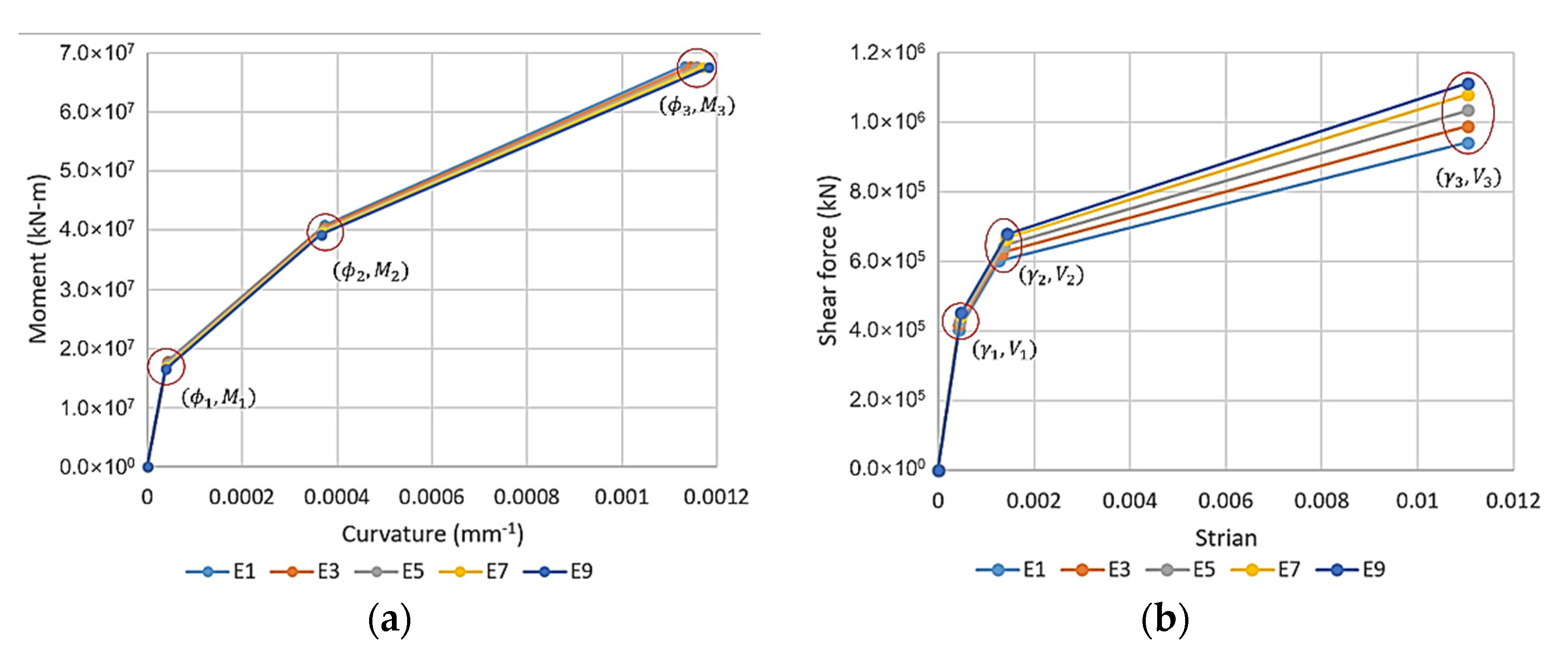
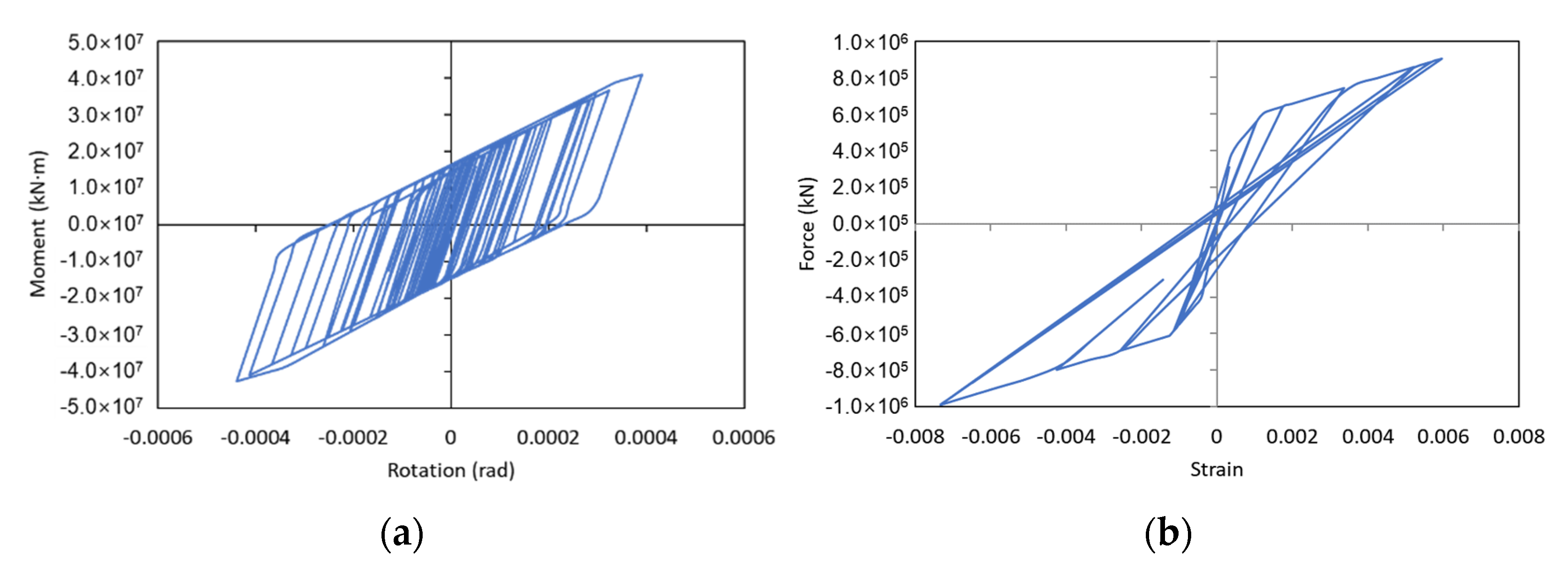
2.2. Nonlinear Modeling

The inelastic behavior of the containment building is modeled based on the methodology proposed by Choi et al. (2006) [2,3]. Plastic hinges were placed at the support and nodes between the beam elements to represent the inelastic flexural deformation. In addition, inelastic shear deformation springs were inserted at the midpoint of each beam-column. Inelastic modeling was limited only to cylindrical walls consisting of the lower part of the structure, and the upper dome was assumed to be elastic considering the seismic force distribution in the vertical cantilever-type structure.

Table 2. Medians and logarithmic standard deviations of modeling parameters.

Modeling Parameter	Median Value	Logarithmic Standard Deviation [1]
$F_c$ (MPa)	41.4	0.14
${ϵ}_c$	0.002	0.17
$F_t$ (MPa)	3.41	0.13
$E_c$ (MPa) 1)	30,241	0.07
$\mathit{G}$ (MPa) 1)	12,096	0.07
$F_y$ (MPa)	455	0.06
$E_s$ (MPa)	200,000	0
$F_{py}$ (MPa)	1810	0.06
$E_p$ (MPa)	193,000	0
Shear strength equation	1	0.16
Damping ratio (%)	0.05	0.35

¹⁾ The elastic modulus of concrete $E_c$ was calculated as $4700\sqrt{F_C}$ and the shear modulus of concrete was calculated as $0.4E_c$.

summarizes the median values of the material properties applied to the inelastic model. In Table 2, $F_c$, $F_y,$ and$F_{py}$ are the compressive and tensile strengths of concrete and the yield strengths of rebars and tendons, respectively, and ${ϵ}_c$ is the strain at the peak stress of concrete. $E_c$, $G$, $E_s$, and $E_p$ are the elastic and shear moduli (MPa) of concrete and the elastic moduli of rebars and tendons, respectively. Two adjacent elements were grouped as a single element group, to which the same plastic hinge property was assigned, and the load–deformation curves for the five beam element groups from the bottom are plotted in Figure 2.

The load–deformation curves for the plastic hinge of beam elements have a tri-linear shape in accordance with the model proposed in JEAG 4604-1987 [24]. These curves for five elements are shown in Figure 2a. In the triangular load–deformation curve, $M_1$ is the moment at the tensile crack of concrete, $M_2$ is the moment corresponding to the first yielding of the outermost reinforcements, and $M_3$ is the moment at the ultimate curvature suggested in JEAG 4604-1987 [24]. The three points defining the trilinear load–deformation curve were determined based on the inelastic bending moment-curvature relationship obtained through inelastic cross-sectional analysis. The material models of concrete and rebars proposed by Mander [25] were adopted, and the increase in strength after yielding was due to strain hardening of the rebars. The degrading trilinear model [24] was adopted to represent the hysteretic behavior of the plastic hinge.

The inelastic shear deformation of the cylindrical wall was modeled using a trilinear load–deformation curve, as shown in Figure 2b, for the same elements as in Figure 2a. The strengths of the two points corresponding to the cracking and yield strengths were calculated using Equations (1) and (2) with reference to JEAG 4604-1987 [24]. For the extreme strength defining the third point, Equation (3) for the ultimate strength of the prestressed cylindrical walls proposed by Ogaki et al. (1981) was adopted [26].

$${\mathsf{\tau }}_1=\sqrt{0.313\sqrt{F_c}\left(0.313\sqrt{F_c}+{\sigma }_m\right)} \left(\mathrm{MPa}\right)$$

(1)

$${\mathsf{\tau }}_2=1.5\times {\mathsf{\tau }}_1$$

(2)

$${\mathsf{\tau }}_3=0.664\sqrt{F_c}+{\left(\rho F_y\right)}_{AVER}\le 1.75\sqrt{F_c} \left(\mathrm{MPa}\right)$$

(3)

where

$${\left(\rho F_y\right)}_{AVER}=\frac{{\rho }_h+{\rho }_m}{2}{F}_y+\frac{{\rho }_{ph}+{\rho }_{pm}}{2}{F}_{py}-\frac{{\sigma }_h+{\sigma }_m}{2} \left(\mathrm{MPa}\right)$$

(4)

In the above equations, ${\rho }_h$ and${\rho }_m$ denote the reinforcement ratios for the rebars in the circumferential and vertical directions, respectively. ${\rho }_{ph}$ and${\rho }_{pm}$ denote the reinforcement ratios for the tendons in the circumferential and vertical directions, respectively. Additionally, ${\sigma }_h$ and ${\sigma }_m$ denote the stress (MPa) in the circumferential and vertical directions generated by the dead load and internal pressure, respectively. The shear strains of the first two points of the skeleton curve are defined as ${\gamma }_1={\tau }_1/G$ and ${\gamma }_2=3{\gamma }_1$, respectively, where $G$ is the shear modulus of concrete. The shear strain ${\gamma }_3$ at the third point is the allowable shear strain, as described later. The effective shear area for converting the shear stress in the load–deformation curve to shear force is defined as follows:

$$A_{eff}=\frac{\pi \times D_c\times t_w}{\alpha }$$

(5)

where $D_c$ and $t_w$ denote the diameter of the centerline of the wall thickness and the thickness of the wall, respectively, and $\alpha$ is the effective shear cross-sectional area coefficient, as defined by Equations (6) and (7).

$$\alpha =2.0, \frac{M}{V{D}_o}\le 0.5$$

(6)

$$\alpha =2.5, \frac{M}{V{D}_o}\le 0.5$$

(7)

where $D_o$ denotes the outer diameter of the circular wall, and $M$ and $V$ denote the bending moment and shear force of the wall, respectively, which were calculated from a linear static analysis assuming a seismic force distribution based on the fundamental vibration mode in this study. A peak-oriented hysteresis model was adopted for the inelastic shear-deformation spring [24]. Examples of hysteresis behavior in a flexural plastic hinge and an inelastic shear deformation spring are shown in Figure 3a,b, respectively.

2.3. Limit State

The limit state of the prestressed concrete wall adopted for the seismic fragility assessment of the NPP containment building in this study is Limit State C, defined in ASCE 43-05 and representing the occurrence of limited permanent deformation [27]. The critical deformation of the limit state is defined by the median and logarithmic standard deviations recommended by EPRI 3002012994 [1]. EPRI 3002012994 classifies shear walls subjected to in-plane deformation as bending-controlled walls if the aspect ratio, $h_w/l_w$, is greater than or equal to 2.0, where $h_w$ and $l_w$ are the height and horizontal length of the wall, respectively. Walls with different aspect ratio are regarded as shear-controlled walls. The aspect ratio of the containment building was 1.58 and the structure was classified as a shear-controlled wall if $l_w$ was defined as the outer diameter of the cylindrical wall and the upper dome was included in the height. However, the part of the cylindrical wall subjected to in-plane deformation is ambiguous considering the shape of the wall. Therefore, both limit states, of which one is for bending and the other is for shear, were considered in this study. The lateral drift ratio to check the limit state of the bending deformation was calculated based on the lateral displacement measured at the boundary between the cylindrical portion and upper dome, considering that the critical drift ratio prescribed in ASCE 43-05 is the inter-story drift ratio, and the containment building does not have a story distinguished by a slab [27]. The shear deformation of the containment building was considered as the maximum shear strain from the individual beam elements.

Table 3. Median and logarithmic standard deviation of allowable drift ratio for limit state [1].

Category		Median Allowable Drift Ratio	Logarithmic Standard Deviation
Bending controlled walls	$V_{ave}>0.50\sqrt{{f_c}^{\prime }}\left(\mathrm{MPa}\right)$	0.007	0.34
	$V_{ave}<0.25\sqrt{{f_c}^{\prime }}\left(\mathrm{MPa}\right)$	0.009
Shear controlled walls		0.007

summarizes the median acceptance criteria for limit states.

3. Ground Motion

3.1. UHRS

First, a UHRS, the basis of CS, was derived for the site of the example containment building. The UHRS was derived from previous studies based on seismic source model A among the four models presented by the Korea Atomic Energy Research Institute (KAERI, 2012) and corresponds to 1/10,000 of the annual excess frequency in Gori, Gyeongsangnam-do [28]. The ground motion prediction equation (GMPE) proposed by Atkinson and Moore (2006) for the Middle East region of the United States and the shear wave velocity, $V_{s30}=760 \mathrm{m}/\mathrm{s},$ was applied to the PSHA [29]. Regarding soil-structure interaction (SSI), dominant frequencies in a coupled soil-structure system may considerably change from those of the structure system decoupled from the soil. The CS is strongly dependent on the control frequency, for which a frequency dominating seismic response is usually chosen. To limit factors affecting seismic response to only structural behavior such as modal contribution and inelastic deformation, SSI was excluded in this study.

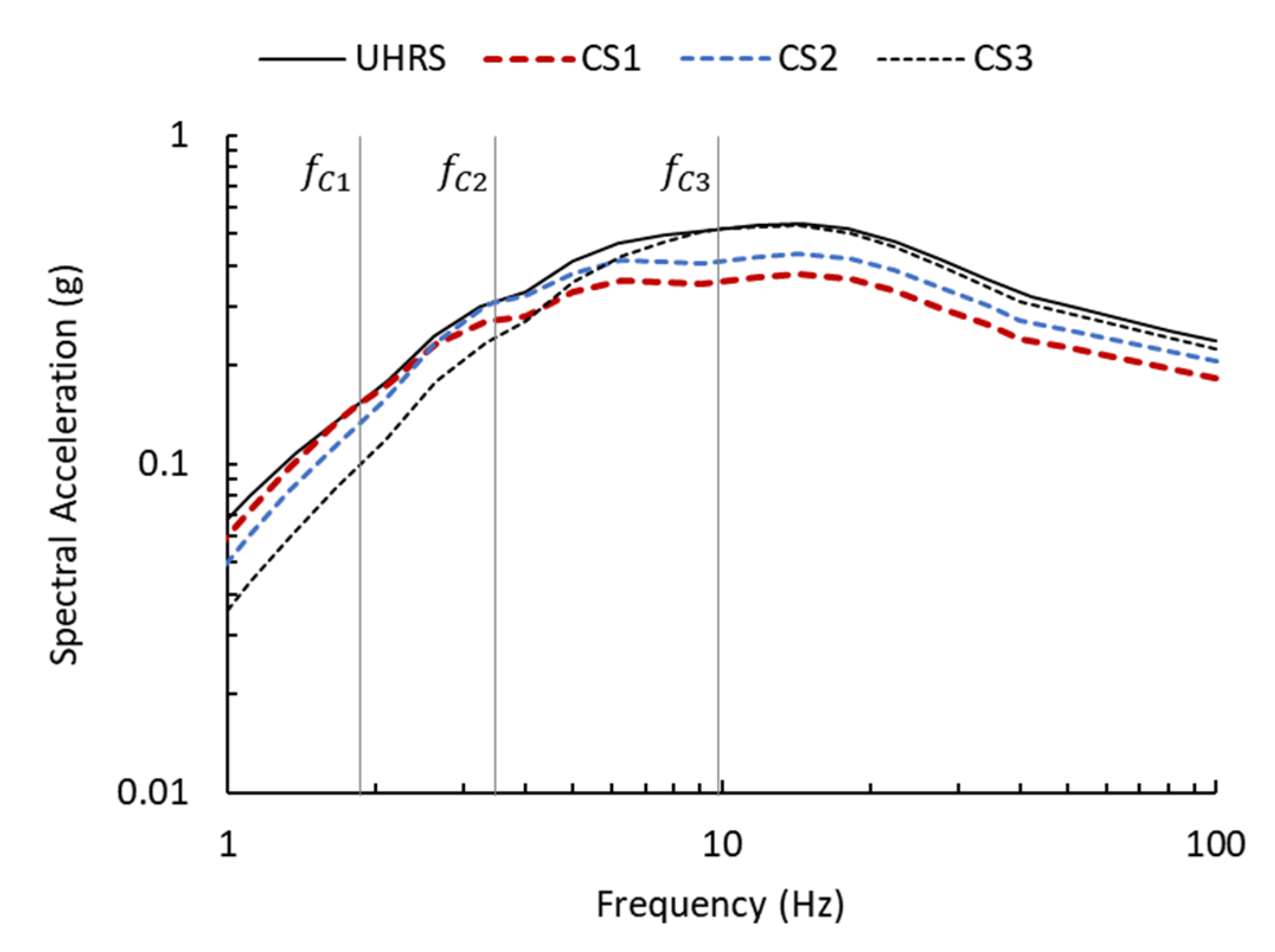
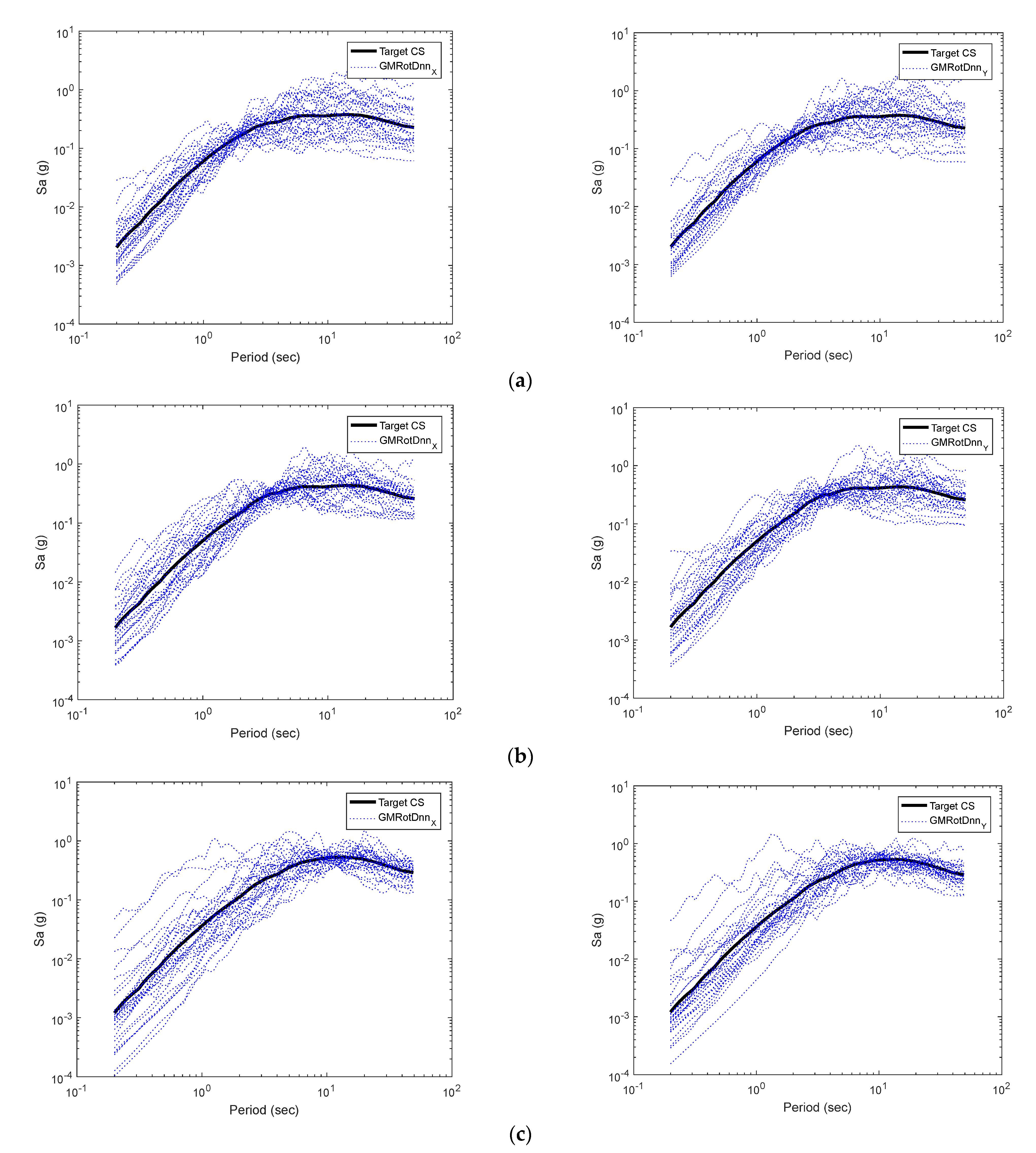
3.2. Conditional Spectrum

The CS was computed based on the dominant earthquake magnitude and epicentral distance determined by the deaggregation of the PSHA at the control frequency and the corresponding spectral acceleration shared by the reference UHRS. The CS is significantly affected by the control frequency. This study adopted a total of three control frequencies. The first control frequency, $f_{c1}$, is half the first modal frequency, the second control frequency,$f_{c2}$, is the first modal frequency, and the third control frequency, $f_{c3}$, is the second modal frequency. The first control frequency, $f_{c1}=1.85 \mathrm{Hz}$, is an approximately half of $f_{c2}$ and reflects a decrease in stiffness owing to the inelastic behavior of the containment building subjected to ultimate deformation, although it was not determined in a quantitative manner. Hereafter, the CS derived for the three control frequencies, $f_{c1}$, $f_{c2},$ and $f_{c3}$ are denoted as CS1, CS2, and CS3, respectively.

Table 4. Control frequencies and corresponding spectral accelerations for conditional spectra.

Response Spectrum for Seismic Input	Control Frequency (Hz)	Spectral Acceleration (g)	$\mathit{r}$, Number of PGA in UHRS 1)
CS1	1.85	0.153	0.648
CS2	3.47	0.311	1.318
CS3	9.96	0.517	2.191

¹⁾ PGA is 0.236 g at 100 Hz in the reference UHRS. See Section 5.2 and Section 5.6 on the usage of $r$.

summarizes the control frequencies and corresponding spectral accelerations.

In a CS, the correlation between the spectral accelerations, of which one is at the control frequency and other frequencies, is defined using the epsilon coefficient, which indicates how much higher the spectral acceleration at the control frequency is compared to the median spectral acceleration predicted by the GMPEs used in the PSHA [6]. Therefore, the construction of a CS requires information on the magnitude and epicentral distance characterizing the dominant earthquake scenario identified by the deaggregation of the seismic hazard at the control frequency. Contribution of the magnitude-epicentral distance combination obtained by the deaggregation of the seismic hazard at the control frequency for each CS is represented in Figure 4. It was observed that the contribution of the scenario with a low magnitude and close distance increased as the control frequency increased. Although the scenario with magnitude 6.2 to 6.4 and epicentral distance 0 to 20 km contributes the most significantly, the proportion of the total is only 13.3 to 13.6%, which is difficult to regard as the single dominant scenario. This is because the seismic source model used in the PSHA was a type of area seismic source with a constant annual rate of exceedance for the earthquake magnitude over the entire area. Therefore, it is necessary to consider various scenarios besides the one with the maximum contribution to the calculation of the CS. In this study, the median and standard deviation of the CS, assumed to be lognormally distributed, were calculated by summing the contributions of all the scenarios shown in Figure 4, based on the methodology proposed by Lin et al. (2013) [30]. Figure 5 shows the median spectra of CS1, CS2, and CS3 along with the UHRS. It was observed that each CS was in contact with the UHRS at the control frequency.

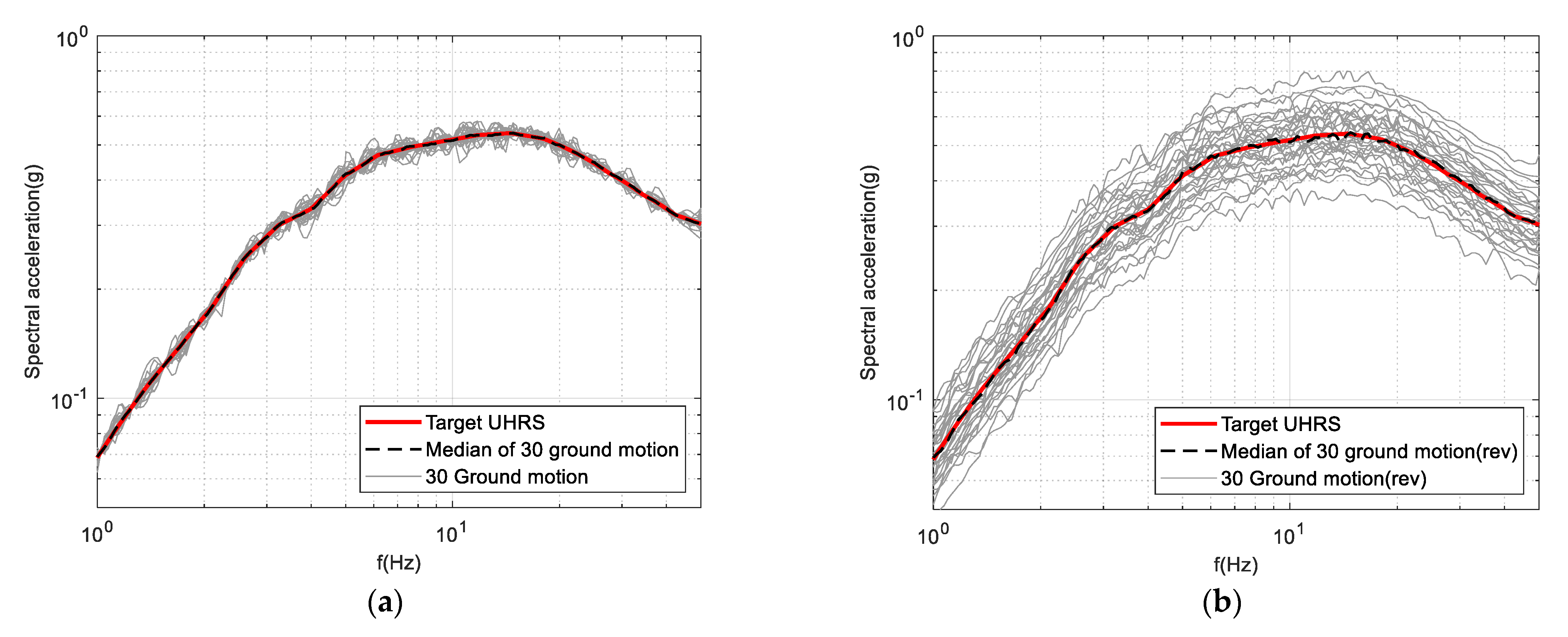
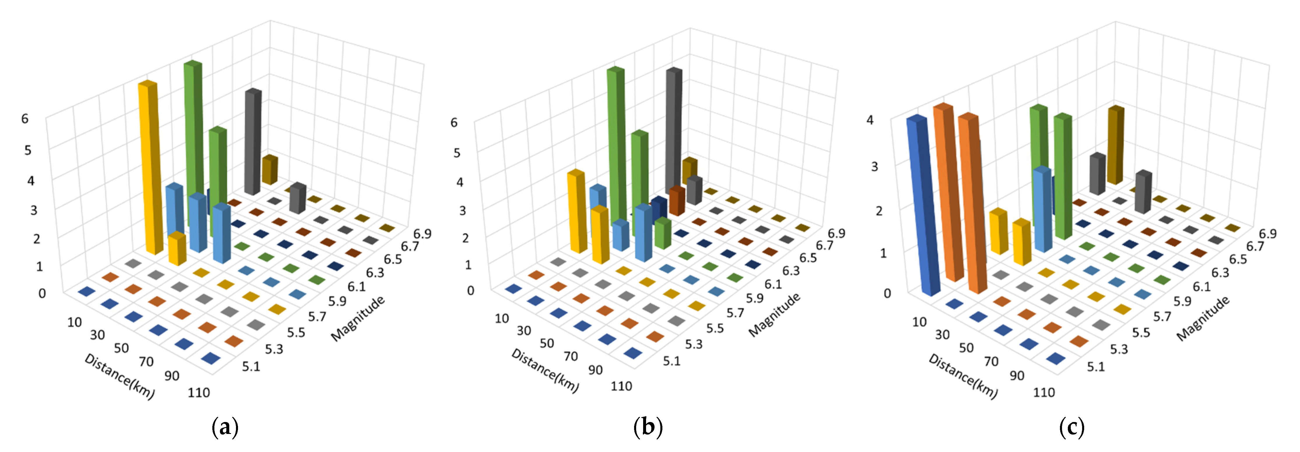
3.3. Ground Motion Time History

Four suites of ground motion records that matched the four target spectra (UHRS, CS1, CS2, and CS3) were prepared. Each suite comprised 30 pairs of horizontal ground motions in orthogonal directions. For the UHRS, randomness due to peaks and valleys in the spectral shape was neglected under the premise that such randomness was already reflected in the PSHA. Thus, the waveform of the ground motion records was modified using a spectral matching procedure [31]. The ground motion suite for CS2, described below, was used as the seed motion for spectral matching with the UHRS. Spectral matching was conducted in accordance with requirement “Option 2: Multiple Sets of Time Histories” of SRP 3.7.1 [32]. The response spectra of the modified ground motion records matched the target UHRS well, as compared in Figure 6a.

In general, the spectral acceleration of a CS at a frequency other than the control frequency is different from that of the reference UHRS and is assumed to be distributed lognormally, as described in Section 3.2. Virtual response spectra simulating the distribution of spectral acceleration for the CS were generated using the algorithm proposed by Jayrem and Baker (2011) [33]. Ground motion records that matched each simulated spectrum were selected from the PEER strong ground motion database [34], and only amplitude scaling was performed without modifying the frequency content. Ground motion records with magnitudes in the range 5.5–7.0 and an epicentral distance of 0 to 50 km were selected based on the result of deaggregation represented in Figure 4. For CS3, the lower bound of magnitude was reduced to 5.0 considering the contribution of magnitudes 5.0 to 5.5, as shown in Figure 4c. The distributions of magnitude and epicentral distances for the selected ground motion records are presented in Figure 7. Because the ground motion records were selected based on the degree of conformity with the shape of the target spectrum, the distribution of the magnitude and epicentral distance was somewhat different from the result of the deaggregation shown in Figure 4. Figure 8 shows the distribution of the GM_RotD50 spectra, a type of geometric mean spectra [35], for the scaled ground motion suite in comparison with the median, 2.5%, and 97.5% confidence levels of the target CS plotted in thick and broken red lines. The thick black broken line represents the median of the response spectra for the scaled ground-motion suite. The median and variance of the target CS were realized using the scaled ground motion suite.

4. Seismic Fragility Assessment Procedure

4.1. Modeling of Randomness

The randomness considered in the SPRA in this study is related to ground motion in two ways. First, the variability of the spectral shape was considered when constructing the target spectra for the three CS and neglected for the UHRS, as described in Section 3.3. Second, the horizontal component-to-component directional variability, which represents the difference between the spectral acceleration in one of the two orthogonal directions and that of the target spectrum, defined as a geometric mean, was considered. To represent this variability for the ground motions matched to the UHRS, one horizontal component was multiplied by $F_H$ whereas the other component orthogonal to the former was divided by the same $F_H$. Consequently, the geometric mean of the two modified ground motion components did not change. $F_H$ conformed to a lognormal distribution with a median of 1.0 and a standard deviation of 0.18 in accordance with EPRI 3002012994 [1]. The spectral distribution of the H1 component for 30 ground motions is shown in Figure 6b. Similarly, the target spectra defined by CS are also defined as a geometric mean. However, in contrast to the UHRS, ground motion records were modified by amplitude scaling only so that the response spectra already had unintentional variability. To introduce directional variability more strictly into the CS, the spectral acceleration at the control frequency was calculated for each ground motion pair by rotating the two orthogonal axes in the horizontal plane from 1° to 180° at 1°. Thirty equally spaced percentiles, ranging from 0 to 100, were randomly assigned to 30 ground motion pairs. Then, each ground motion was rotated by an angle corresponding to the randomly chosen percentile of the spectral acceleration in the H1 axis and applied to a three-dimensional dynamic analysis. The spectral distributions of the H1- and H2-components of 30 scaled ground motion pairs with randomly rotated orientations are plotted in Figure 9.

4.2. Modeling of Uncertainty

The uncertainties in the material properties, shear strength equations, limit state criteria, and damping ratio are reflected in the SPRA in this study. Each parameter with an uncertainty was assumed to follow a lognormal distribution, for which the logarithmic standard deviations recommended in EPRI 3002012994 were adopted [1]. Table 2 presents the logarithmic standard deviations for each modeling variable. The uncertainty in the shear strength formula was represented by multiplying ${\tau }_3$, calculated by Equation (3), by a random number, and ${\tau }_1$ and ${\tau }_2$ were multiplied by the same coefficient to reflect the variability proportionally. For the acceptance criteria, the logarithmic standard deviations due to randomness and uncertainty are 0.15 and 0.30, respectively, as per EPRI 3002012994 [1]. In this study, they were combined by the square root of the sum of squares (SRSS) combination rule and the resultant 0.34 was assigned to the uncertainty for convenience in modeling and analysis, as given in Table 3. Thirty sets of modeling variables, identical to the number of ground motion pairs in a suite, were derived using the Latin hypercube sampling (LHS) technique [36]. The load–deformation curves for the bending and shear deformations of the beam elements at the bottom using each set of random modeling variables are plotted in Figure 10a,b, respectively. The load–deformation curves for bending have relatively low variability compared with those for shear, to which uncertainty in the shear strength equations was additionally applied. Hereafter, the model reflecting variability in modeling variables is designated by ‘LHS model’.

4.3. Incremental Dynamic Analysis

An incremental dynamic analysis (IDA) was performed to derive seismic fragility curves [37]. It would be ideal to derive different response spectra and ground motion suites corresponding to each seismic hazard level adopted in incremental dynamic analysis. However, considering the effort required to select and adjust ground motion records, IDA was performed by scaling the ground motion suite matched to the intensity of the representative seismic hazard level corresponding to the annual frequency of exceedance, 1/10,000 [1]. For the UHRS, scale factors from 0.8477 to 25.43, which lead to a median PGA of 0.2 to 6.0 g, were applied to records in the ground motion suite identically. The spectral acceleration at 100 Hz was deemed to be the PGA for the UHRS. The scale factors used in the UHRS case were applied to the ground motion suite for the CS, considering that the target CS has the same level of seismic hazard as the UHRS at the control frequency, as shown in Figure 5.

5. Probabilistic Seismic Risk Assessment Result

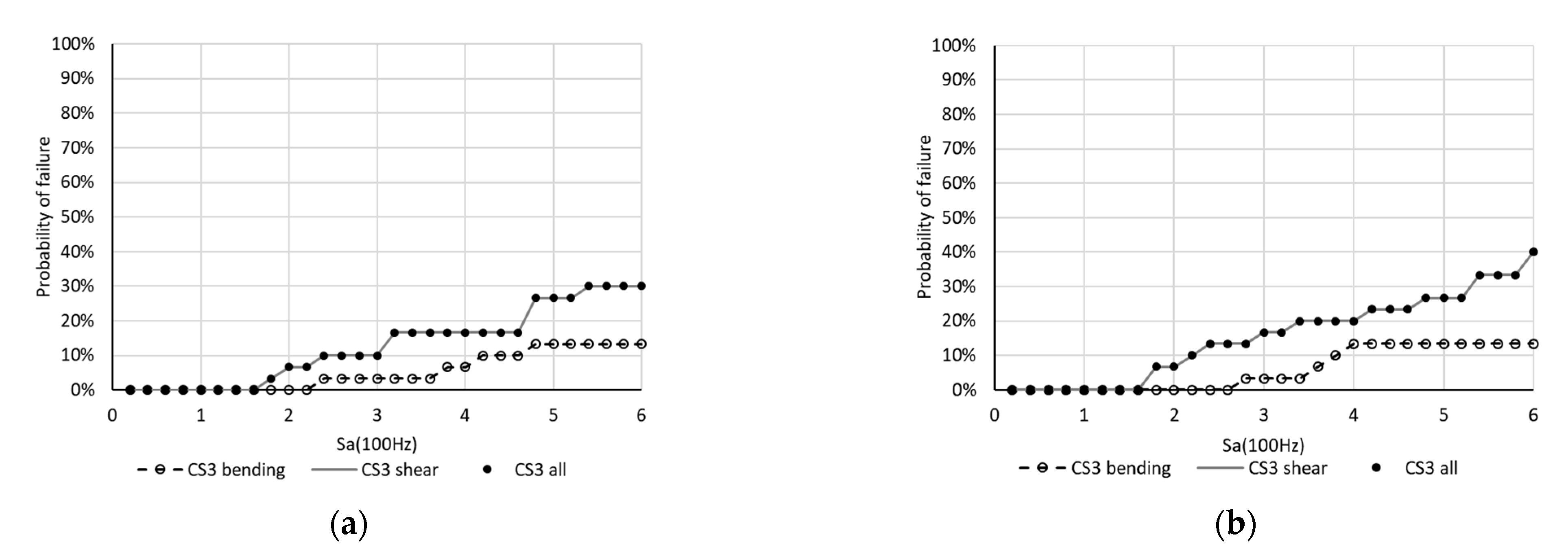
5.1. Contribution of Limit States

In the incremental dynamic analysis, the two limit states for bending and shear were checked, and the contribution of each limit state was examined. Figure 11 shows the probability of failure induced by bending, shear, and both bending and shear from the IDA for ground motion based on CS3. The probability of failure by shear completely overlaps that by both bending and shear for both the median and LHS models. The same tendency is observed in IDA for ground motion based on other reference spectra, such as UHRS, CS1, and CS2. Therefore, all the seismic fragility curves derived below were consistently governed by the limit state of shear deformation.

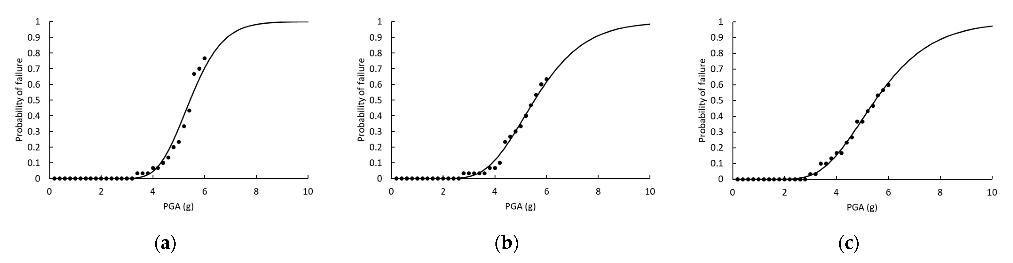
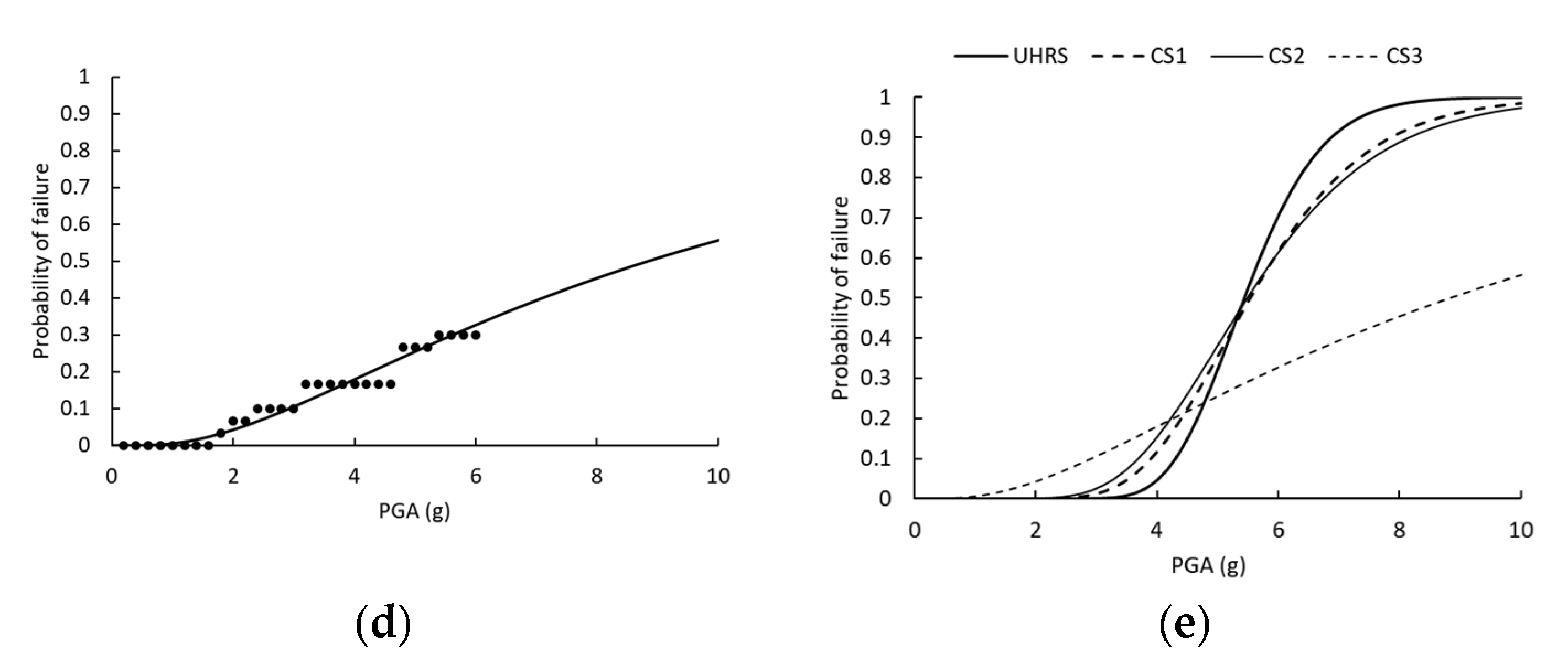
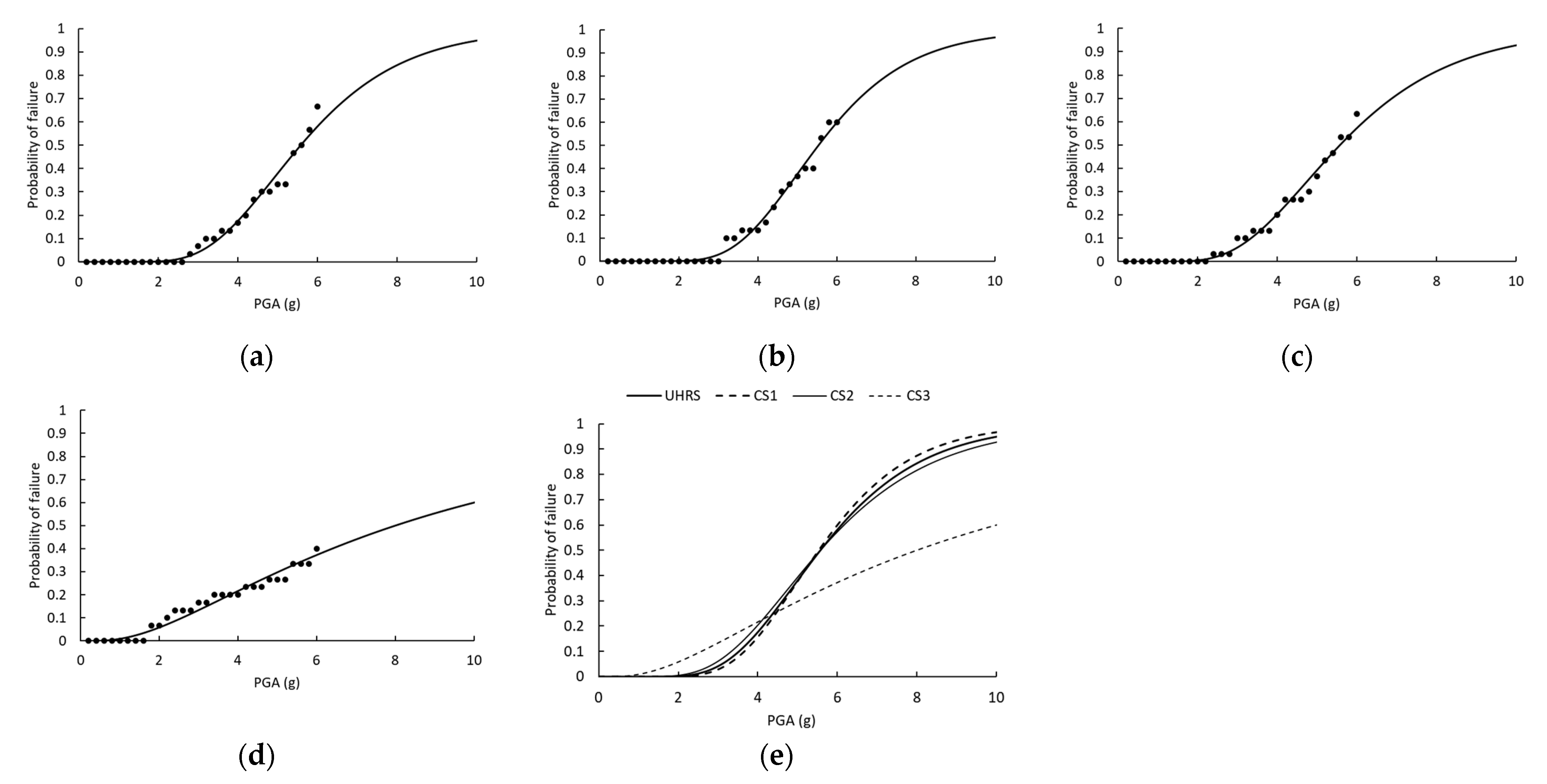
5.2. Seismic Fragility Curve

The intensity of the ground motion was unified to compare the seismic fragility curves obtained from the ground motion defined by the different types of response spectra. Although a single CS and the corresponding UHRS have the same spectral acceleration at the control frequency, it was impossible to use the spectral acceleration at the control frequency as a unified intensity measure, considering that the three conditional spectra, CS1, CS2, and CS3, have different control frequencies. Instead, the PGA of the UHRS was adopted as a unified intensity measure of the ground motion. The ratio between the spectral acceleration at the control frequency of the CS and PGA of the UHRS (contacting the CS at the control frequency) is presented in the last column of Table 4, which can be used to convert the PGA-based seismic fragility curve into a seismic fragility curve defined by the spectral acceleration at the control frequency.

A seismic fragility curve in the form of a lognormal distribution was derived based on the frequency of exceeding the limit state criteria for shear obtained from IDA. Although the analysis was performed up to a PGA of 6.0 g, the probability of failure reached up to 70% only. The maximum likelihood method proposed by Baker (2014) was used to estimate the median and standard deviation of the lognormal distribution by using a limited range of samples [38].

Table 5. Median capacity and logarithmic standard deviation.

Seismic Input Model	Median Capacity (g)		Logarithmic Standard Deviation
	Median Model	LHS Model	Median Model	LHS Model
	${\mathit{A}}_{\mathit{m}}$		${\mathit{\beta }}_{\mathit{R}}$	${\mathit{\beta }}_{\mathit{C}}$	${\mathit{\beta }}_{\mathit{U}}$
UHRS	5.44	5.57	0.183 1)	0.357 1)	0.307
CS1	5.54	5.53	0.273	0.322	0.171
CS2	5.49	5.57	0.310	0.401	0.255
CS3	8.83	8.00	0.864	0.883	0.183

¹⁾ ${\beta }_{PV,R}$ = 0.0395 was removed based on the SRSS rule.

summarizes the median PGA and lognormal standard deviation of each seismic fragility curve. The seismic fragility curves obtained using different seismic input models are plotted in Figure 12 and Figure 13 for the median and LHS models of the containment building, respectively. To confirm the suitability of the seismic fragility curve in each figure, the probability of failure calculated for each step of the IDA is plotted with circles in Figure 12 and Figure 13. A good agreement between the raw data and the curve can be seen. Comparison among fragility curves is given in Figure 12e and Figure 13e for median and LHS models, respectively. It is observed that the order of the probability of failure changes between the median and LHS models due to difference in logarithmic standard deviations. The fragility curves based on UHRS and CS1 has the lowest probability of failure in the low PGA region for median and LHS models, respectively.

5.3. Median Capacity

The median value of the seismic fragility curve represents the intensity measure of ground motion for which a structure fails at 50% probability. The values of the median intensity measure, defined as PGA and denoted by $A_m$, are listed in Table 5. For the median model, the median value is in the range 5.44 to 5.54 g for UHRS, CS1, and CS2, and increases to 8.83 g for CS3. The increase in the median value for CS3 is due to the significantly lower spectral acceleration than that of the other response spectra at the primary modal frequency, which controls the response of the structure, as shown in Figure 5. For the LHS model, the median value of UHRS, CS1, and CS2 ranges from 5.53 to 5.57 g, and the median value of CS3 is 8.00 g, which is similar to the median model.

5.4. Logarithmic Standard Deviation

The logarithmic standard deviations of the different fragility curves are summarized in Table 5. The logarithmic standard deviation, ${\beta }_R$, obtained from the median model reflects only the randomness of the seismic input. The logarithmic standard deviation, ${\beta }_C$, obtained from the LHS model reflects both the randomness of the seismic input and the uncertainty in modeling and limit state criteria. The logarithmic standard deviation ${\beta }_U$, which represents variability due to uncertainty, was calculated from ${\beta }_C$ and ${\beta }_R$ based on the SRSS combination rule, ${\beta }_C=\sqrt{{\beta }_R^2+{\beta }_U^2}$. For the UHRS-based seismic input model, the variability of the response spectra with respect to the target spectrum remaining after spectral matching, as observed in Figure 6, was removed from ${\beta }_R$ based on the SRSS rule [1], where the spectral variability denoted as ${\beta }_{PV,R}$ was determined by averaging the logarithmic standard deviations of the spectral acceleration with respect to frequencies. The value of ${\beta }_{PV,R}$ was very small relative to the value of ${\beta }_R$ and had a negligible effect. Consequently, the ${\beta }_R$ listed for the UHRS-based seismic input model can be viewed as randomness owing to only the horizontal component-to-component directional variability. On the other hand, the three CS-based seismic input models include randomness owing to the variability of the spectral shape, as shown in Figure 8, in addition to the component-to-component directional variability represented in Figure 9.

The logarithmic standard deviations,${\beta }_R,$ calculated for the median model are 0.183, 0.273, 0.310, and 0.864 for UHRS, CS1, CS2, and CS3, respectively. CS-based seismic input models generally produce larger ${\beta }_R$ than UHRS-based seismic inputs. This is because CS reflects an additional source of randomness, that is, spectral shape variability, compared with UHRS. In particular, the value of ${\beta }_R$ from the response to the UHRS-based seismic input is almost the same as the logarithmic standard deviation of the directional variability factor $F_H$. In addition, for the CS-based seismic input models, ${\beta }_R$, decreases at a lower control frequency. This is because the dominant frequency of the structure moved from $f_{c2}$ to $f_{c1}$ as the inelastic deformation of the structure became more significant, and randomness in the CS-based ground motion suites tended to be minimal in the vicinity of the control frequency. For the CS1-based seismic input, ${\beta }_R$ is 0.273, which is similar to the logarithmic standard deviation of the spectral acceleration, 0.24 to 0.25, at the control frequency summarized in

Table 6. Logarithmic standard deviation for the spectral acceleration at control frequency.

Direction	Seismic Input Model
	CS1	CS2	CS3
H1	0.24	0.24	0.24
H2	0.25	0.23	0.24

. However, ${\beta }_R$s for CS2 and CS3 were significantly higher than the corresponding standard deviations in Table 6 because the spectral variability at the dominant frequency increased as the control frequency was located far from the dominant frequency. It is noted that the logarithmic standard deviations for CSs in Table 6 are unique to the individual seismic input model but the logarithmic standard deviation, 0.18, for $F_H$ is a generic characteristic of UHRS. Therefore, it is expected that the ${\beta }_R$s for the CS would have decreased somewhat if the spectral variability at the control frequency had been adjusted to 0.18, as for the UHRS.

The logarithmic standard deviation$, {\beta }_C$, calculated for the LHS models includes the influence of both randomness and uncertainty. The CS1-based seismic input model has the smallest ${\beta }_C$ of 0.322 among all the seismic input models, as shown in Table 6. As a result, ${\beta }_U$s calculated based on ${\beta }_C$ and ${\beta }_R$ using the SRSS rule, ${\beta }_C=\sqrt{{\beta }_R^2+{\beta }_U^2}$, for all three CSs are smaller than the UHRS value, and ${\beta }_U$ for CS1 is the smallest. That is, CSs tend to yield higher ${\beta }_R$ and lower ${\beta }_U$ compared with the UHRS. The spectral acceleration of the UHRS in Figure 5 decreases as the frequency moves in the frequency range from$f_{c2}$ to $f_{c1}$ owing to the inelastic deformation of the structure. In this study, ${\beta }_U$ is the response variability caused by the model uncertainty including uncertainty in the natural frequency. For the UHRS, the response spectral acceleration changes in phase with the change of the fundamental frequency of the model. However, for CS2, the median spectral acceleration in Figure 5 is always lower than that of the UHRS, so that the effect of natural frequency variability on the response variability is reduced compared to that of the UHRS. For CS1, the slope of the spectrum between $f_{c1}$ and $f_{c2}$ lower than that of the UHRS results in lower response variability. For CS3, the magnitude of the logarithmic standard deviation representing multiplicative variability decreases because the median value is much higher than that of other seismic input models. In summary, the logarithmic standard deviations, ${\beta }_R$ and ${\beta }_U$, of the seismic fragility curve for the CS-based seismic input model can be reduced by adopting a control frequency lower than the primary modal frequency corresponding to the expected inelastic behavior of the structure.

5.5. HCLPF Capacity

The HCLPF of the containment building was calculated based on the median and logarithmic standard deviations of the individual seismic fragility curves. The HCLPF is the ground motion level at which there is a low probability of failure with a high confidence. The low probability of failure is defined as 5% non-exceedance probability of the ground motion level that follows a lognormal distribution with a standard deviation, ${\beta }_R$. The ground motion level has a median value with a high confidence, that is, 95% exceedance probability subjected to a lognormal distribution with a lognormal standard deviation, ${\beta }_U$ [1]. The HCLPF is defined by Equation (8). In addition, HCLPF′, which is the minimum of HCLPF approximated by 1% probability of failure, was calculated using Equation (9) [1].

$$\mathrm{HCLPF}=A_m{e}^{-1.65\left({\beta }_R+{\beta }_U\right)}$$

(8)

$${\mathrm{HCLPF}}^{\prime }=A_m{e}^{-2.33{\beta }_C}$$

(9)

where $A_m$ is the median capacity obtained from the median model; and${\beta }_R$, ${\beta }_U$, and ${\beta }_C$ are the logarithmic standard deviation due to randomness, the logarithmic standard deviation due to uncertainty, and the combined logarithmic standard deviation, respectively.

The HCLPF and HCLPF’ values, calculated based on the variables presented in Table 5, are summarized in

Table 7. HCLPF and HCLPF’ capacities in PGA (parenthesis: normalized with UHRS).

Seismic Input Model	$\mathbf{H}\mathbf{C}\mathbf{L}\mathbf{P}\mathbf{F}$	${\mathbf{H}\mathbf{C}\mathbf{L}\mathbf{P}\mathbf{F}}^{\prime }$
UHRS	2.442 (1.00)	2.378 (1.00)
CS1	2.663 (1.09)	2.615 (1.10)
CS2	2.162 (0.89)	2.156 (0.91)
CS3	1.569 (0.64)	1.128 (0.47)

. Here, the values in the parentheses are normalized to the corresponding values of the UHRS. Compared with UHRS, the HCLPF value for CS1 increases by 9%, while the HCLPF’ values for CS2 and CS3 decrease by 11% and 36%, respectively. HCLPF’ has a tendency similar to that of HCLPF. The difference in HCLPF or HCLPF’ for various seismic input models is caused by the difference in the logarithmic standard deviation considering that the median capacities of the UHRS, CS1, and CS2 are similar, as shown in Table 5. As a result, the HCLPF or HCLPF’ can be assessed more reasonably by using a CS-based seismic input model, and it is necessary to choose a control frequency predominant in the inelastic structural behavior to reduce the effect of randomness in the seismic input.

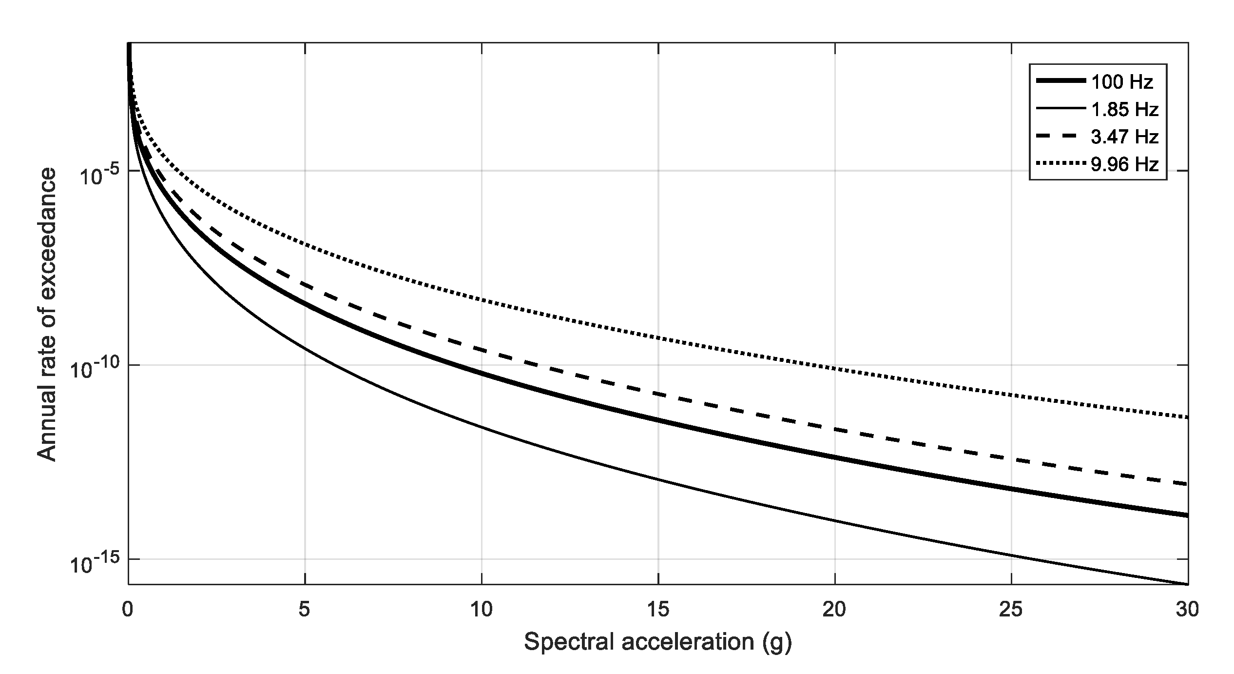
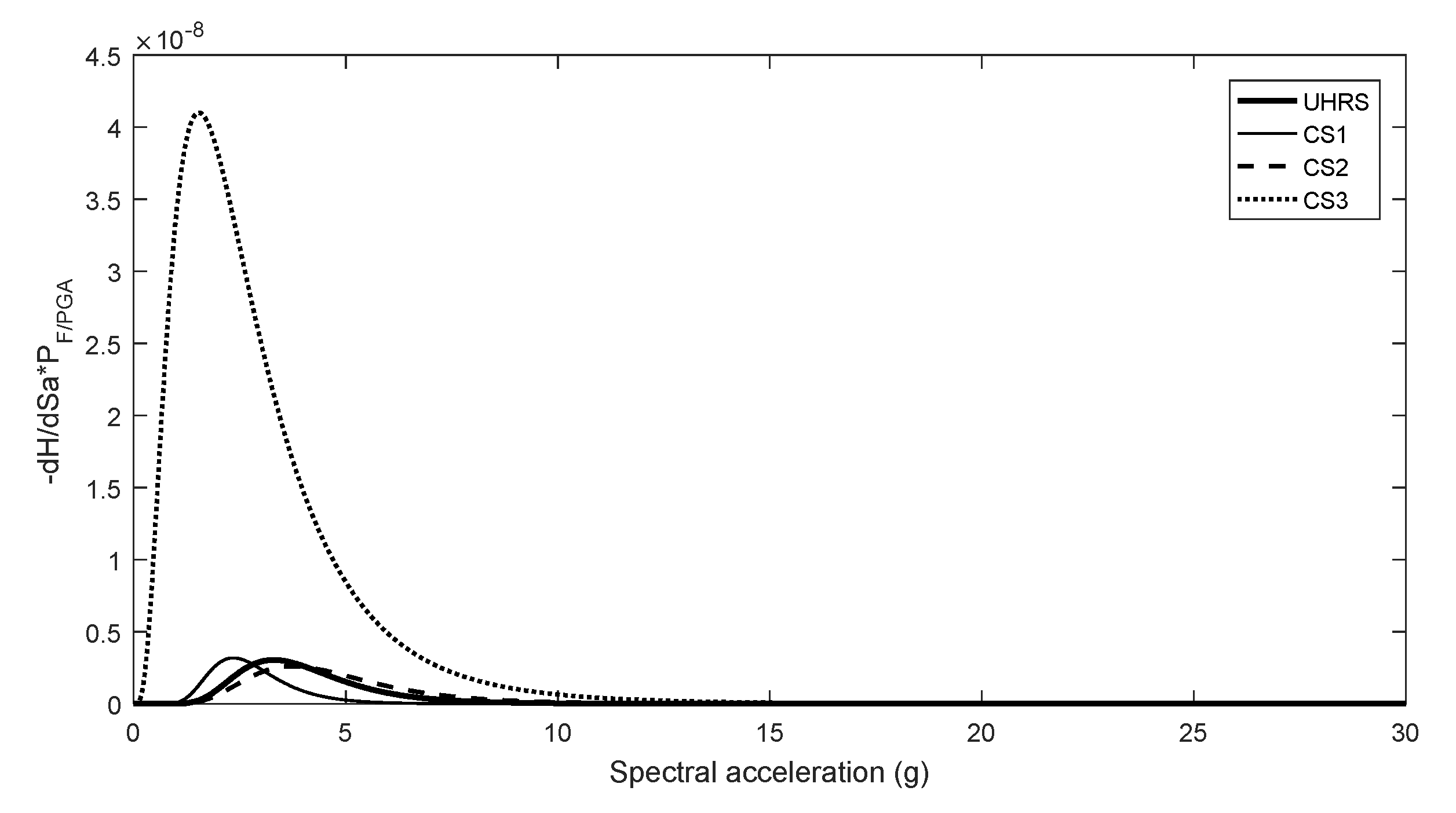
5.6. Probabilistic Seismic Risk

To evaluate the seismic risk of the containment building, the probability of failure (PF) was calculated by convolving the seismic fragility curve and probability density function (PDF) derived from the seismic hazard curve as follows:

$$P_F=-{{\displaystyle \int }}_0^{\infty }\left(\frac{dH\left(a_f\right)}{d{a}_f}\right)P_{F/a_f}\left(a_f\right)d{a}_f=-{{\displaystyle \int }}_0^{\infty }\left(\frac{dH\left(a_f\right)}{d{a}_f}\right)P_{F/PGA}\left(a_f/r\right)d{a}_f$$

(10)

where $a_f$ is the intensity measure defining the seismic hazard curve, which is the PGA for the UHRS and the spectral acceleration at $f_c$ for the CS. $P_{F/a_f}$ is the seismic fragility curve defined as the conditional probability of failure when a specific value of $a_f$ occurs. $P_{F/PGA}$ is the seismic fragility curve presented in Figure 13, and all of them were defined by PGA, which was substituted with the spectral acceleration at 100 Hz in this study. To unify the convolution variables, the PGA was represented by$a_f$ using the following equation:

$$PGA=a_f/r$$

(11)

where $r$ is the conversion factor listed in the last column of Table 4, based on the spectral accelerations for a return period of 10,000 years. The hazard curve for the spectral acceleration at 100 Hz and the three control frequencies, CS, is plotted in Figure 14, and the integrand of Equation (10) representing the probability density of failure is shown in Figure 15.

Table 8. Seismic risk of APR 1400 containment building for given seismic hazard curve.

Hazard Curve	Fragility Curve
	${\mathit{P}}_{\mathit{F},\mathit{U}\mathit{H}\mathit{R}\mathit{S}}$	${\mathit{P}}_{\mathit{F},\mathit{C}\mathit{S}1}$	${\mathit{P}}_{\mathit{F},\mathit{C}\mathit{S}2}$	${\mathit{P}}_{\mathit{F},\mathit{C}\mathit{S}3}$
H (100 Hz)	0.955 × 10−8	-	-	-
H (1.85 Hz)	0.812 × 10−8	0.658 × 10−8	-	-
H (3.47 Hz)	0.727 × 10−8	-	1.01 × 10−8	-
H (9.96 Hz)	0.769 × 10−8	-	-	13.2 × 10−8

summarizes the calculated failure probabilities. For UHRS, it is not rational to select a single curve among seismic hazard curves defined at different frequencies because the UHRS has the same probability of exceedance for each frequency. Therefore, the UHRS-based seismic fragility curve was convolved with the seismic hazard curve for 100 Hz and the three control frequencies respectively. Moreover, the CS-based seismic hazard curve was convolved with the seismic hazard curve for the corresponding control frequencies.

Among the four PFs for the UHRS-based fragility curve, the maximum PF is 0.955 × 10⁻⁸ at 100 Hz, and the minimum PF is 0.727 × 10⁻⁸ at 3.47 Hz. However, the PF of the CS-based seismic fragility curve has a value from 0.658 × 10⁻⁸ to 13.2 × 10⁻⁸ depending on the control frequency. The PF for the CS-based fragility curve has a larger discrepancy depending on the control frequency than the PF for the UHRS-based curve. The minimum PF in Table 8 is 0.658 × 10⁻⁸ for CS1, which corresponds to: (a) 81% of 0.812 × 10⁻⁸, the PF for the UHRS-based seismic fragility curve at 1.85 Hz, calculated using the same hazard curve H (1.85 Hz); and (b) 91% of 0.727 × 10⁻⁸, which is the minimum of the four $P_{F,UHRS}$s calculated for different frequencies. In particular, the $P_{F,CS1}$ is only 69% of 0.955×10^-8, the$P_{F,UHRS}$ obtained using H (100 Hz), a conventional PGA-based seismic hazard curve. Therefore, through the use of CS, the ambiguity in the selection of the seismic hazard curve is eliminated, and the PF may be reduced compared to the UHRS by selecting a control frequency that can minimize the effect of randomness in the seismic input model.

6. Conclusions

In this study, a procedure for the seismic fragility assessment of NPPs by applying ground motion compatible with the probability distribution of CS was presented with a case study for the containment building of an NPP. To this end, three CSs was defined for three control frequencies, and ground motions were selected and scaled to simulate the conditional probability distribution of spectral acceleration. Horizontal component-to-component directional variability was considered as a source of randomness, in addition to spectral shape variability. Nonlinear LMS models were constructed using parameters determined by the LHS to model uncertainty. The seismic fragility curves were calculated from the IDA for seismic inputs based on the CS and compared with those obtained using a conventional seismic input based on the UHRS. The conclusions of this study are summarized as follows.

(1)

By selecting a control frequency close to the dominant frequency in the structural response, the seismic input model based on the CS produces a similar median capacity compared to the UHRS-based seismic input model and reduces the logarithmic standard deviation due to randomness.

(2)

When a CS-based seismic input is applied to structural models simulating uncertainty, the randomness due to seismic input accounts for a large proportion of the combined logarithmic standard deviation, and the proportion of uncertainty decreases compared with the UHRS-based seismic input.

(3)

When the CS-based seismic input with a control frequency close to the dominant frequency is adopted, the HCLPF capacity is enhanced, and the probability of failure is reduced considerably compared with the result from the UHRS-based seismic input.

(4)

In addition, the CS-based seismic input has an advantage in that the basis for selecting the seismic hazard curve for seismic risk assessment is clear.

(5)

Spectral shape variability and component-to-component variability are important sources of randomness that characterize the CS and need to be introduced in a rigorous manner as applied to UHRS.

For the application of the CS to the practical SPRA of NPPs based on the findings of this study, it is necessary to develop detailed guidelines that addresses the issues of selecting the control frequency and strictly matching ground motions with prescribed component-to-component variability. Additionally, although this study was conducted using a simple inelastic LMS model, the seismic fragility and risk assessment of NPP structures using CSs can be conducted using more rigorous FE models that account for inelastic behavior directly or indirectly using inelastic energy absorption factors.

References

1. EPRI. Seismic Fragility and Seismic Margin Guidance for Seismic Probabilistic Risk Assessments; EPRI 3002012994; EPRI: Palo Alto, CA, USA, 2018. [Google Scholar]
2. Choi, I.K.; Ahn, S.M.; Choun, Y.S. Seismic Fragility Analysis of PSC Containment Building by Nonlinear Anaysis. Earthq. Eng. Soc. Korea 2006, 10, 63–74. [Google Scholar]
3. Choi, I.K.; Choun, Y.S.; Ahn, S.M.; Seo, J.M. Probabilistic Seismic Risk Analysis of CANDU Containment Structure Near-Fault Earthquakes. Nucl. Eng. Des. 2008, 238, 1382–1391. [Google Scholar] [CrossRef]
4. Kim, M.K.; Choi, I.K. Effect of Evaluation Response Spectrum on the Seismic Risk of Structure. Earthq. Eng. Soc. Korea 2009, 13, 39–46. [Google Scholar]
5. Hahm, D.; Seo, J.M.; Choi, I.K.; Rhee, H.M. Uniform Hazard Spectrum Evaluation Method for Nuclear Power Plants on Soil Sites based on the Hazard Spectra of Bedrock Sites. Earthq. Eng. Soc. Korea 2012, 16, 35–42. [Google Scholar] [CrossRef] [Green Version]
6. Baker, J.W. Conditional Mean Spectrum: Tool for Ground-Motion Selection. J. Struct. Eng. 2011, 137, 322–331. [Google Scholar] [CrossRef]
7. ASCE/SEI 7-16. Minimum Design Loads and Associated Creteria for Buildings and other Structures; American Society of Civil Engineers: Reston, VA, USA, 2017. [Google Scholar]
8. Haselton, C.B.; Baker, J.W.; Stewart, J.P.; Whittaker, A.S.; Luco, N.; Fry, A.; Hamburger, R.O.; Zimmerman, R.B.; Hooper, J.D.; Charney, F.A.; et al. Response History Analysis for the Design of New Buildings in the NEHRP Provisions and ASCE/SEI 7 Standard: Part Ⅰ—Overview and Specification of Ground Motions; Earthquake Engineering Research Institute: Seoul, Korea, 2017; Volume 33, pp. 373–395. [Google Scholar]
9. Haselton, C.B.; Fry, A.; Hamburger, R.O.; Baker, J.W.; Zimmerman, R.B.; Luco, N.; Elwood, K.J.; Hooper, J.D.; Charney, F.A.; Pekelinicky, R.G.; et al. Response History Analysis for the Design of New Buildings in the NEHRP Provisions and ASCD/SEI 7 Standard: Part Ⅱ—Structural Aanlysis Procedures and Acceptance Criteria; Earthquake Engineering Research Institute: Seoul, Korea, 2017; Volume 33, pp. 397–417. [Google Scholar]
10. Jarrett, J.A.; Zimmerman, R.B.; Charney, F.A.; Jalalian, A. Response—History Analysis for the Design of New Buildings in the NEHRP Provisions and ASCE/SEI 7 Sthandard: Part Ⅳ-A Study of Assumptions; Earthquake Engineering Research Institute: Seoul, Korea, 2017; Volume 33, pp. 449–468. [Google Scholar]
11. Zimmerman, R.B.; Baker, J.W.; Hooper, J.D.; Bono, S.; Haselton, C.B.; Engel, A.; Hamburger, R.O.; Celikbas, A.; Jalalian, A. Response History Analysis for the Design of New Buildings in the NEHRP Provisions and ASCD/SEI 7 Standard: Part Ⅲ—Example Applications Illustrating the Recommended Methodology. Earthquake Engineering Research Institute: Seoul, Korea, 2017; Volume 33, pp. 419–447. [Google Scholar]
12. Renault, P. PEGASOS refinement project: New findings and challenges from a PSHA for Swiss Nuclear Power Plants. In Proceedings of the Transactions, SMiRT 21, New Delhi, India, 6–11 November 2011. [Google Scholar]
13. Renault, P.; Kurmann, D. Comparison of uniform hazard spectra and conditional spectra approach in the framework of fragility curve development. In Proceedings of the Transactions, SMiRT 22, San Francisco, CA, USA, 18–23 August 2013. [Google Scholar]
14. Renault, P.; Proske, D.; Kurmann, D.; Asfura, A.P. Evaluation of the seismic risk of a NPP building using the conditional spectra approach. In Proceedings of the Transactions, SMiRT 23, Manchester, UK, 10–14 August 2015. [Google Scholar]
15. Renault, P.; Asfura, A.P. Comarison of approaches for selecting and adjusting time histories to be used in seismic fragility analyses. In Proceedings of the Transactions, SMiRT 25, Charlotte, NC, USA, 4–9 August 2019. [Google Scholar]
16. Reed, J.W.; Kennedy, R.P. Methodology for Developing Seismic Fragilities; EPRI TR-103959; Electric Power Research Institute: Palo Alto, CA, USA, 1994. [Google Scholar]
17. Cho, H.; Koh, H.M.; Hyun, C.H.; Shin, H.M. Seismic damage assessment of nuclear power plant containment structures. In Proceedings of the 13th World Conference on Earthquake Engineering, Vancouver, BC, Canada, 1–6 August 2004; Volume 2972, pp. 1–6. [Google Scholar]
18. Tavakkoli, I.; Kianoush, M.R.; Abrishami, H.; Han, X. Finite element modelling of a nuclear containment structure subjected to high internal pressure. Int. J. Press. Vessels Pip. 2017, 153, 59–69. [Google Scholar] [CrossRef]
19. Nguyen, D.D.; Thusa, B.; Park, H.; Azad, M.S.; Lee, T.H. Efficiency of various structural modeling schemes on evaluating seismic performance and fragility of APR1400 containment building. Nuclear Eng. Technol. 2021, 53, 2696–2707. [Google Scholar] [CrossRef]
20. Li, Z.; Guo, J.; Jin, S.; Zhang, P.; Gong, J. Fragility analysis and probabilistic safety evaluation of the nuclear containment structure under different prestressing loss conditions. Ann. Nuclear Energy 2022, 167, 108862. [Google Scholar] [CrossRef]
21. Korea Electrical Power Corporation; Korea Hydro & Nuclear Power Co., Ltd. APR1400 DESIGN CONTROL DOCUMENT TIER2. APR1400- K-X-FS-14002-NP REVISION 0; Korea Electrical Power Corporation: Busan, Korea; Korea Hydro & Nuclear Power Co., Ltd.: Gyeongju-si, Korea, 2014. [Google Scholar]
22. Park, W.H. Seismic Fragility Analysis of Nuclear Power Plant Containment Structures Based on Conditional Spectrum; Incheon National University: Incheon, Korea, 2019. [Google Scholar]
23. Available online: https://www.midasuser.com/ (accessed on 27 April 2022).
24. Japan Electric Association (JEA). Technical Guidelines for a Seismic Design of Nuclear Power Plants: Translation of JEAG 4601-1987, JEAG-4601; Japan Electric Association: Tokyo, Japan, 1991. [Google Scholar]
25. Chang, G.A.; Mander, J.B. Seismic Energy Based Fatigue Damage Analysis of Bridge Columns: Part 1—Evaluation of Seismic Capacity; NCEER Technical Rep. No. NCEER-94-0006; State University of New York: Buffalo, NY, USA, 1994. [Google Scholar]
26. Ogaki, Y.; Kobayashi, M.; Takeda, T.; Yamaguchi, T.; Yoshizaki, K.; Sugano, S. Shear strength tests of prestressed concrete containment vessels. In Proceedings of the SMiRT-6, Paris, France, 17–21 August 1981; Volume 13. [Google Scholar]
27. American Society of Civil Engineers. Seismic Design Criteria for Structures, Systems, and Components in Nuclear Facilities; ASCE/SEI 43-05; American Society of Civil Engineers: Reston, VA, USA, 2005. [Google Scholar]
28. Korea Atomic Energy Research Institute. Development of Ground Response Spectrum for Seismic Risk Assessment; Korea Meteorological Administration: Seoul, Korea, 2018; p. 171.
29. Atkinson, G.M.; Boore, D.M. Earthquake Ground-Motion Prediction Equations for Eastern North America. Bull. Seismol. Soc. Am. 2006, 96, 2181–2205. [Google Scholar] [CrossRef]
30. Lin, T.; Harmsen, S.C.; Baker, J.W.; Luco, N. Conditional spectrum computation incorporating multiple causal earthquakes and ground motion prediction models. Bull. Seismol. Soc. Am. 2013, 103, 1103–1116. [Google Scholar] [CrossRef]
31. Al Atik, L.; Abrahamson, N.A. An improved method for non-stationary spectral matching. Earthq. Spectra 2010, 26, 601–617. [Google Scholar] [CrossRef] [Green Version]
32. US Nuclear Regulatory Commission. US Nuclear Regulatory Commission Standard Review Plan 3.7.1; Revision 4. NUREG-0800; U.S. Nuclear Regulatory Commission: Washington, DC, USA, 2014.
33. Jayaram, N.; Lin, T.; Baker, J.W. A Computationally Efficient Ground—Motion Selection Algorithm for Matching a Target Response Spectrum Mean and Variance. Earthq. Spectra 2011, 27, 797–815. [Google Scholar] [CrossRef]
34. PEER Ground Motion Database. Available online: https://ngawest2.berkeley.edu/ (accessed on 27 April 2022).
35. Boore, D.M.; Watson-Lamprey, J.; Abrahamson, N.A. Orientation-independent measures of ground motion. Bull. Seismol. Soc. Am. 2006, 96, 1502–1511. [Google Scholar] [CrossRef]
36. Helton, J.C.; Davis, F.J. Latin hypercube sampling and the propagation of uncertainty in analyses of complex systems. Reliab. Eng. Syst. Saf. 2003, 81, 23–69. [Google Scholar] [CrossRef] [Green Version]
37. Vamvatsikos, D.C.; Cornell, C.A. Incremental dynamic analysis. Earthq. Eng. Struct. Dyn. 2002, 31, 491–514. [Google Scholar] [CrossRef]
38. Baker, J.W. Efficient analytical fragility function fitting using dynamic structural analysis. Earthq. Spectra 2014, 31, 579–599. [Google Scholar] [CrossRef]
Figure 1. Numerical model of the containment building: (a) 3D finite element model; (b) Lumped mass stick model.
Applsci 12 05176 g001
Figure 2. Median load–deformation curves for five inelastic beam element groups, in order from the bottom: (a) Bending; (b) Shear.
Applsci 12 05176 g002
Figure 3. Hysteretic behavior of beam element from nonlinear dynamic analysis: (a) Degrading trilinear for bending; (b) Peak-oriented model for shear.
Applsci 12 05176 g003
Figure 4. Deaggregation of seismic hazard at the control frequency of CS: (a) CS1; (b) CS2; (c) CS3.
Applsci 12 05176 g004
Figure 5. UHRS and median CSs for annual frequency of exceedance = 1/10,000.
Applsci 12 05176 g005
Figure 6. UHRS and spectra for spectrally matched ground motions (H1-component): (a) Initial matching; (b) Scaled for directional variability.
Applsci 12 05176 g006
Figure 7. Distribution of the magnitude and epicentral distance for ground motion suite: (a) CS1; (b) CS2; (c) CS3.
Applsci 12 05176 g007
Figure 8. Distribution of GM_RotD50 spectra of ground motion suite scaled to CS: (a) CS1; (b) CS2; (c) CS3.
Applsci 12 05176 g008aApplsci 12 05176 g008b
Figure 9. Spectral distribution of H1- and H2-components of 30 scaled ground motion pairs with randomly rotated orientation: (a) CS1; (b) CS2; (c) CS3.
Applsci 12 05176 g009
Figure 10. Load–deformation curves of bottom element obtained by LHS: (a) Bending; (b) Shear.
Applsci 12 05176 g010
Figure 11. Probability of failure from IDA for ground motion defined by CS3: (a) Median model; (b) LHS model.
Applsci 12 05176 g011
Figure 12. Seismic fragility curves for median models: (a) UHRS; (b) CS1 with f c f 1 / 2 ; (c) CS2 with f c = f 1 ; (d) CS3 with f c = f 2 ; (e) all fragility curves.
Applsci 12 05176 g012aApplsci 12 05176 g012b
Figure 13. Seismic fragility curves for LHS models: (a) UHRS; (b) CS1 with f c f 1 / 2 ; (c) CS2 with f c = f 1 ; (d) CS3 with f c = f 2 ; (e) all fragility curves.
Applsci 12 05176 g013
Figure 14. Seismic hazard curves for risk evaluation.
Applsci 12 05176 g014
Figure 15. Probability density of failure.
Applsci 12 05176 g015