
Influence of Climate Change and Land-Use Alteration on Water Resources in Multan, Pakistan


1
Department of Civil Engineering, School of Naval Architecture, Ocean and Civil Engineering, Shanghai Jiao Tong University, Shanghai 200240, China
2
Department of Civil and Environmental Engineering, College of Engineering, Shantou University, Shantou 515063, China
3
Guangdong Engineering Center for Structure Safety and Health Monitoring, Shantou University, Shantou 515063, China
*
Authors to whom correspondence should be addressed.
Appl. Sci. 2022, 12(10), 5210; https://0-doi-org.brum.beds.ac.uk/10.3390/app12105210
Submission received: 28 April 2022
/
Revised: 17 May 2022
/
Accepted: 19 May 2022
/
Published: 21 May 2022
(This article belongs to the Special Issue Freshwater Ecological and Environmental Status)
Abstract
:This study presents an evaluation of climate and land-use changes induced impacts on water resources of Multan City, Pakistan. Statistical Down Scaling Model (SDSM) and Geographical Information System (GIS) are used for climate change scenario and spatial analyses. Hydrologic Engineering Center’s Hydraulic Modeling System (HEC-HMS) model is used for rainfall-runoff simulation. The investigated results show significant changes in climatological parameters, i.e., an increase in temperature and decrease in precipitation over the last 40 years, and a significant urban expansion is also observed from 2000 to 2020. The increase in temperature and urbanization has reduced the infiltration rate into the soil and increased the runoff flows. The HEC-HMS results indicate that surface runoff gradually increased over the last two decades. Consequently, the depth of the water table in the shallow aquifer has declined by about 0.3 m/year. Projected climate indices stipulate that groundwater depletion will occur in the future. Arsenic levels have exceeded the permissible limit owing to unplanned urban expansion and open dumping of industrial effluents. The results can help an efficient water resources management in Multan.
1. Introduction
In the context of climate change, the rapid urbanization, population growth, and anthropogenic activities strongly influence the local and global environments. Climate change has been considered the most alarming worldwide issue by climatologists [1]. According to the Intergovernmental Panel on Climate Change (IPCC) fourth assessment report, the global temperature has increased by 0.6–0.8 °C over the last century, which is a record increment over the last 1000 years [2,3]. Recent research stipulates that regular climate changes, intensification of anthropic activities, and rapid urbanization largely affect the water budget of urban areas [4,5,6,7,8]. Global warming has also changed the timing, amount, and distribution of water, causing adverse effects on the water supply system through flooding [9,10,11,12,13,14,15,16] and droughts risks [17]. Similarly, it has been demonstrated that land-use changes such as pavement, urbanization, logging, deforestation, and soil erosion also contribute to influence hydrologic processes such as rate of infiltration, interception, and evapotranspiration [18,19,20]. Due to an increase in impervious surface, the infiltration rate and concentration-time decrease, causing urbanization to yield more surface runoff and peak inflows to river systems [21,22,23].
Multan is among fast-growing cities in Punjab, Pakistan. Over the last 54 years (1960–2013), an average increase of 1.9 °C in the mean lowest temperature has been observed in Punjab province, with a projected increase of 1.4 °C in the following 30 years [24]. Past findings suggest that this extreme climate change stems from mechanisms such as melting glaciers, smog in winter, heatwaves, forest fires in summer, landslides, and population dynamics [24]. The deleterious occurrences of this extreme climate change and extensive land-use have recently brought the city of Multan to national attention, especially given their impact on water resources and their distribution over the region. This points out the need to investigate the combined effect of climate change and land-use on water resources over this area, especially, in the view of the 2030 sustainable development goals (SDG6) defined by the United Nations (https://sdgs.un.org/goals; accessed on 1 January 2021). Indeed, the poor understanding of this effect may result in the sub-optimal management of water resources and put local population at greater risk of freshwater stress and diseases.
Over the last few decades, a sizable number of studies investigated the effects of climate and land-use change on water resources using climate and hydrological models [25,26]. Among them, global climate models (GCMs) have been acknowledged as one of the most effective ways to assess future water resources [27]. The advantage of this approach is that daily archived data simulated from global climate models (GCMs) are readily available for specific time duration [28,29]. Moreover, for the last couple of decades, downscaling methods have been used for future climate projection and long-term weather forecasting [30]. In reality, by coupling GCMs and hydrological models, downscaling methods can be divided into dynamical downscaling and statistical downscaling [31,32]. Statistical downscaling models are computationally convenient and widely used for regional climate change impact evaluation [24,33].
This study presents an approach for the spatiotemporal impact evaluation of land-use and climate on water, and its application to the Multan region, Pakistan. The objective is to seize and assess the patterns of the interactions between climate change, land-use, and water resources for this city, which presents atypical extreme climate change and land-use rate. As such, this study is bound to help relevant authorities in making decisions for sustainable water management. Remote sensing (RS) and geographic information system (GIS) are used for hydrological modeling and land-use change evaluation. Daily temperature and metrological variables are downscaled from daily GCM simulations to particular sites by using a statistical downscaling model (SDSM).
2. Materials and Methods
2.1. Study Area
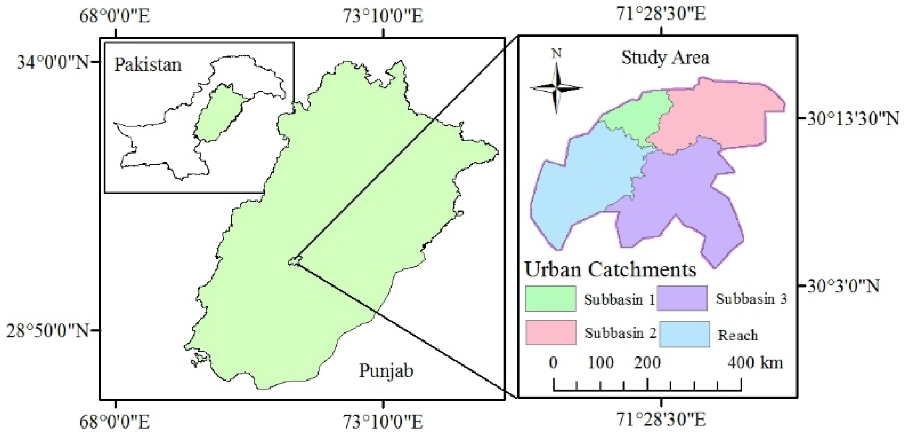
The study area is located in the urban hub of the district of Multan (Multan city), which is the pronounced part of Bari Doab, Punjab plains (Figure 1) [34]. Geographically, it is located in the center of Pakistan, with an elevation of 114 to 135 m above sea level. The area comprises alluvial plains derived by the Indus, Chenab, Sutlej, Jhelum, and Ravi Rivers. The Sutlej and Indus Rivers define the southeastern and western boundaries of the Punjab plains, respectively. The slope of the Punjab plains is to the southwest and varies from 0.366 m per kilometer in the northern part to less than 0.182 m per kilometer in the southern part; the average slopes are 0.274 m per kilometer [34,35,36], and demonstrate that mixed and varied soil patterns exist in the area due to sudden and frequent changes in the streamflow velocities. Most of the soils in Punjab plains have been characterized as moderately to highly permeable, while few areas were found to have a low permeability [37,38].
2.2. Hydrological Framework
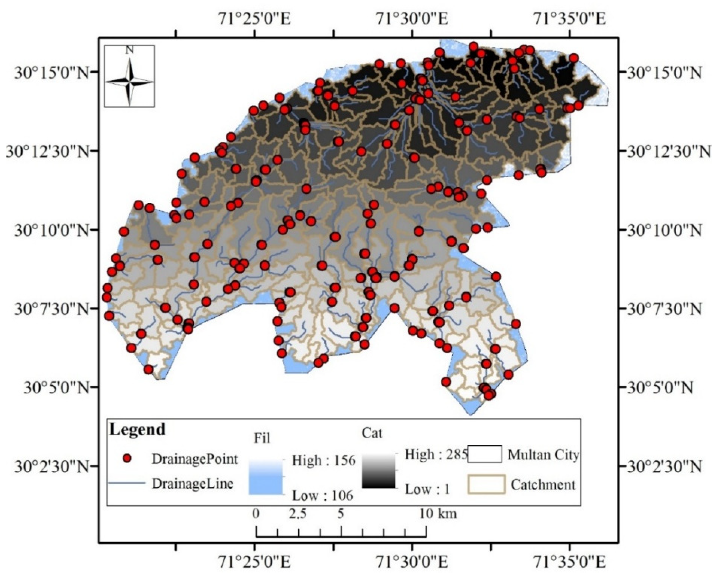
The study area lies on the eastern bank of River Chenab, which has become the only source of groundwater recharge for the area. This River typically consists of braided channels within the city of Multan. The elevation in the south parts is low and starts rising toward the middle and northeastern parts of the study region, where the elevation ranges from 126 to 135 m. This means that the natural surface slope is rising toward the center and northeastern parts. These features were further analyzed using Arc-Hydro tools to reveal the natural surface hydrologic setting of the study area as shown in Figure 2. In this figure, natural drainage points, drainage lines, fil, adjoining catchment, and catchment polygons are principally highlighted.
2.3. Data Collection
The observed daily predictors of National Centre for Environmental Prediction (NCEP), and daily predictors of Global Climate Model (GCM) were gathered from Canadian Government (http://climate-scenarios.canada.ca/?page=pred-hadcm3; accessed on 20 September 2020). Historical daily observed maximum and minimum temperature, precipitation, and other climate variables such as air humidity and wind speed were collected from Pakistan Metrological Department (PMD). Data for depth to the water table and arsenic concentration level were collected from the Punjab irrigation department. Digital Elevation Model (DEM) and Landsat data were downloaded from the earth explorer, USGS (https://earthexplorer.usgs.gov; accessed on 20 September 2020) site.
2.4. Methodology
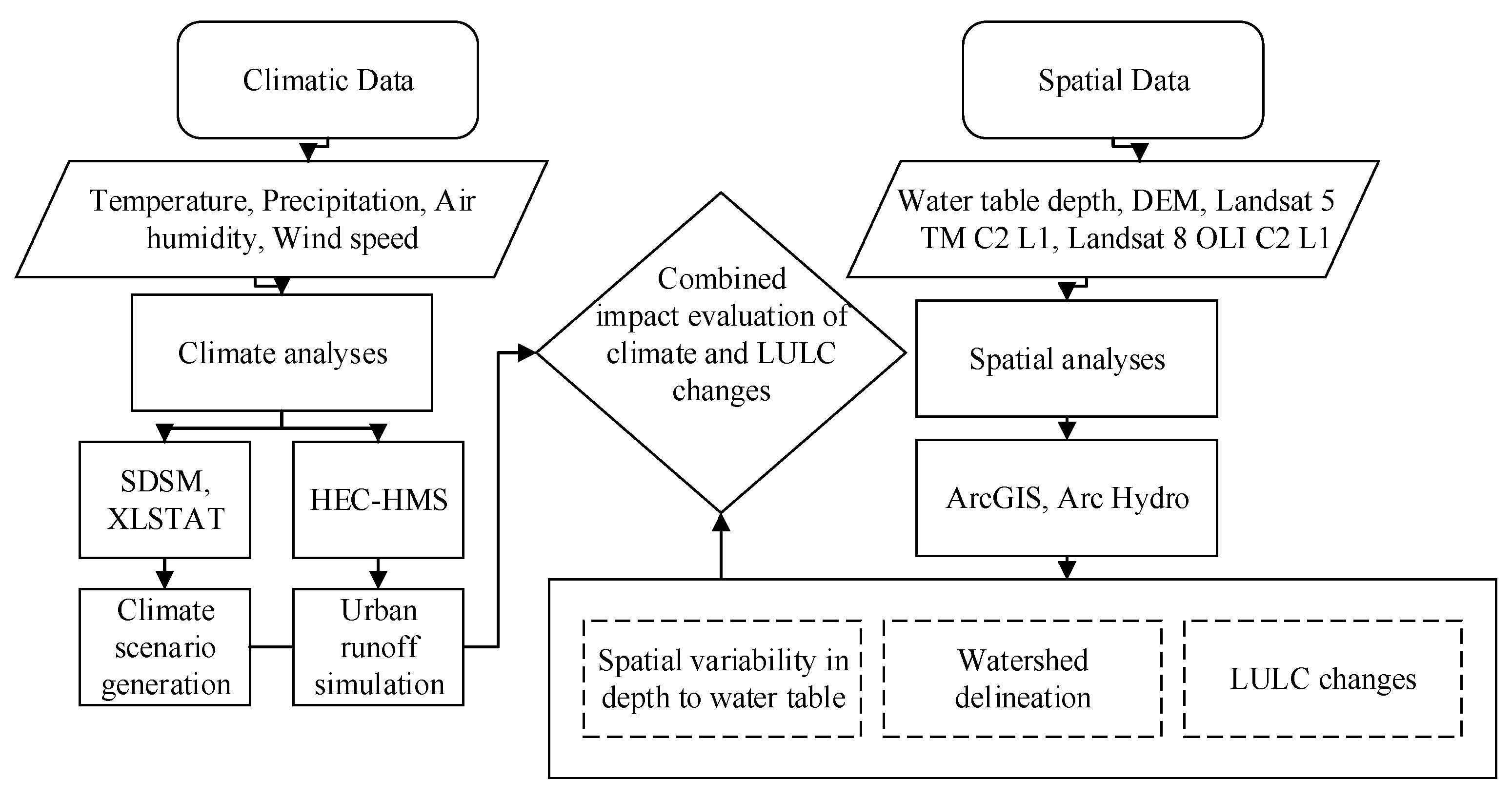
Figure 3 shows the methodological framework of this research. Firstly, Statistical Downscaling Model (SDSM) is used for climate downscaling. Past temperature and precipitation data are used for SDSM calibration and validation using National Centre for Environmental Prediction (NCEP) and Global Climate Models (GCMs) predictors, respectively. Secondly, ArcGIS packages is implemented for hydrological modeling (watershed delineation), and spatial analyses of land-use land cover (LULC) changes. Thirdly, Hydrologic Engineering Center’s—Hydrologic Modeling System (HEC-HMS) model is employed to simulate the runoff by using daily rainfall data from 2000 to 2020. Finally, results from the prior steps are used to evaluate the impact of climate and LULC changes on surface water (i.e., rainfall-runoff), groundwater (i.e., depth to water-table), and water quality (i.e., arsenic concentration level only) of the study area.
2.4.1. Description of SDSM
The SDSM is a coupled Multiple Linear Regression (MLR) and Stochastic Weather Generator (SWG) model developed by [39,40,41,42,43,44]. In this method, statistical and empirical relations between NCEP’s predictors and observed predictands are generated by MLR throughout predictors screening and SDSM calibration processes [45,46,47,48,49]. In this study, the projected climate scenario (Table 1) was determined in the calibration phase through predictor screening. Let us recall that to screen the predictor variables, it is necessary to individually correlate them with the predictands, i.e., precipitation and temperature. Considering this aspect, a conditional sub-model was selected for precipitation to account for wet-day occurrences, whereas an unconditional process was adopted for independent temperature. As a result, predictor variables with a p range of (0 ≤ p ≤ 0.05) were chosen as the best fit correlated predictors for a single predictand. Moreover, using available observed daily data from 1978 to 2000, the model was calibrated and validated for Tmax and Tmin. However, for precipitation downscaling, the NCEP predictors were used for model calibration and GCM predictors for model validation using data of the same period 1990–2001 (details can be found in Section 3.1).
Furthermore, the weather generator process was conducted to produce synthetic daily data by using calibrated output file (*.PAR-extension) and observed NCEP selected predictors variables. It allows the verification of calibrated model using observed data and generated artificial time series for the present status of climate [50]. Lastly, the scenario generation was performed following a procedure analogous to the weather generation process. The only difference between weather generation and scenario generation processes is the H3A2a_1961-2099 file that was selected in the GCM directory for scenario generation (instead of the NCEP_1961-2001 file for weather generation). Scenario generation gives the projected climate predicted variables supplied by the global climate models.
2.4.2. Mann–Kendall Test Method
Addinsoft’s XLSTAT Software was used to perform the statistical Mann–Kendall test. In climatologic and hydrologic time series, the Mann–Kendall test is a widely used statistical approach for trend analysis [51]. In this test, the null hypothesis H0 indicates that there is no trend in the time series and that the data are independent and randomly ordered. Conversely, the alternative hypothesis H1 assumes that there is a trend in the time series. In reality, the null hypothesis H0 is rejected in favor of H1 when p-value exceeds the alpha value (0.050) [51]. Kendall’s parameters were used to analyze the trend of climatologic and hydrologic data. The positive or negative value of Statistic “S” was used to infer an upward or downward trend, while the statistic Kendall’s tau was used to measure the relationship and correlation between two variables.
2.4.3. Supervised Classification of Satellite Imageries and Digital Elevation Model (DEM) Reconditioning
ArcGIS 10.5 was used for the supervised classification of satellite imageries. Specifically, after the image processing, atmospheric corrections, and radiometric calibration steps, the satellite images were used for supervised classification to categorize the study area into different LULC classes [50]. Similarly, Digital Elevation Model (DEM) reconditioning was performed using Arc-Hydro tools for watershed delineation. As a digital visualization of ground surface terrain, DEM contains several hydrological data from which can be extracted relevant surface information such as flow direction or slope, drainage line, and catchment polygons [52].
2.4.4. HEC-HMS Model Setup
HEC-HMS rainfall-runoff simulation model is used to calculate the total outflow of the small urban catchment. The HEC-HMS model simulates the runoff by using rainfall data and other input parameters [53]. The Soil Conservation Service-curve number (SCS-CN) method was used to find the losses for reach’s input parameters. Basically, this method develops a relation between lag time (Tlag) and time of concentration (Tc) to calculate the lag time for each time scenario. In particular, it uses the curve number (CN), which is calculated from hydrological soil and land-use land cover data. In reality, an increase in curve number suggests a decrease in infiltration and an increase in runoff. Once the LULC classes are identified, the next step is to determine the percentage of each hydrological soil group (A–D) in the study area. Then, the curve number (in %) for each class is calculated and summed to give the final value of curve number. Finally, based on the length of the reach and characteristics of the subbasins, the Kirpich formula is used to find the time of concentration as follows:
where S stands for the slope, L represents the Reach length (in ft), and Ia is the Initial abstraction.
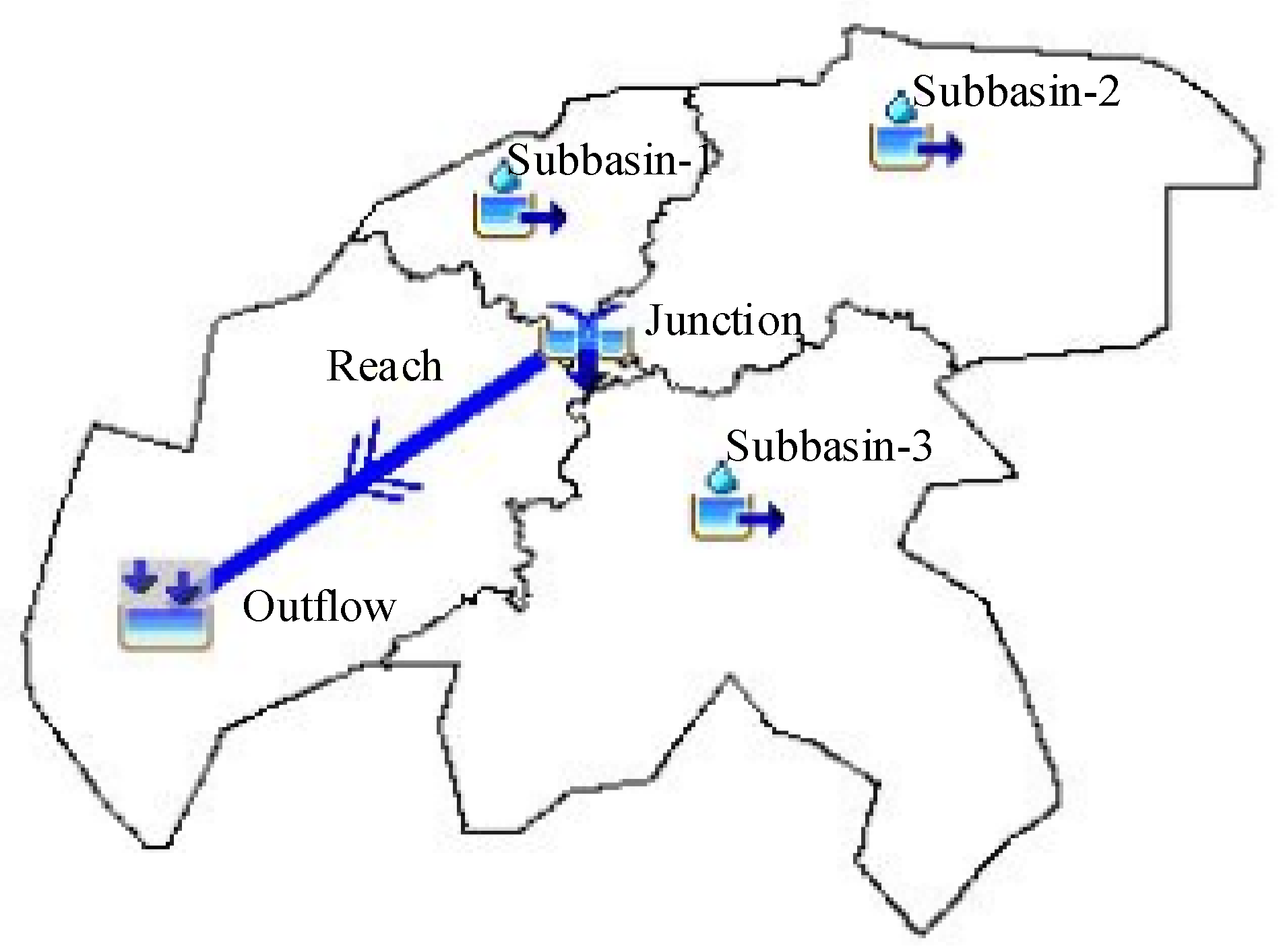
In this study, the urban catchment was divided into three subbasins along with their junction and reach for model input parameters, as shown in Figure 4. Rainfall real-time daily data from 2000 to 2020 were used to run HEC-HMS to simulate the total runoff from all subbasins of the urban catchment [53]. The start and end date of the storm event and the time interval were both provided in the manager component of “Control Specifications” in HEC-HMS model. A 1-day time interval was used for each five-year rainfall scenario from 2000 to 2020. For runoff simulation, the entire period from 1 January 2000 to 31 December 2020 is divided into four five-year scenarios. Hydrographs are obtained as simulation output at every unit (junction, reach, and outflow) of the established model; then hydrographs peaks are used to infer the maximum outflow discharge at junctions.
3. Results and Discussion
3.1. Calibration and Validation of SDSM
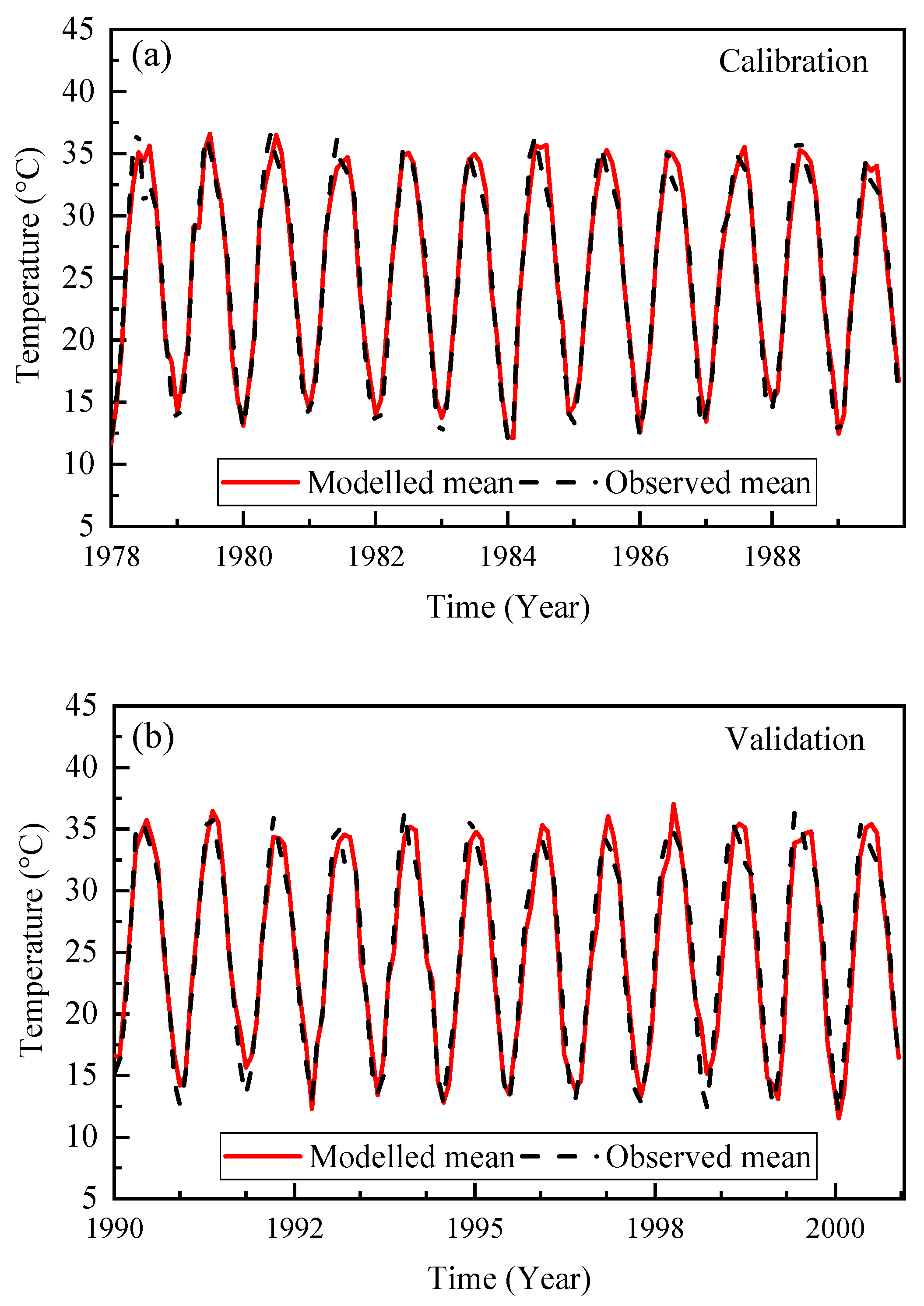
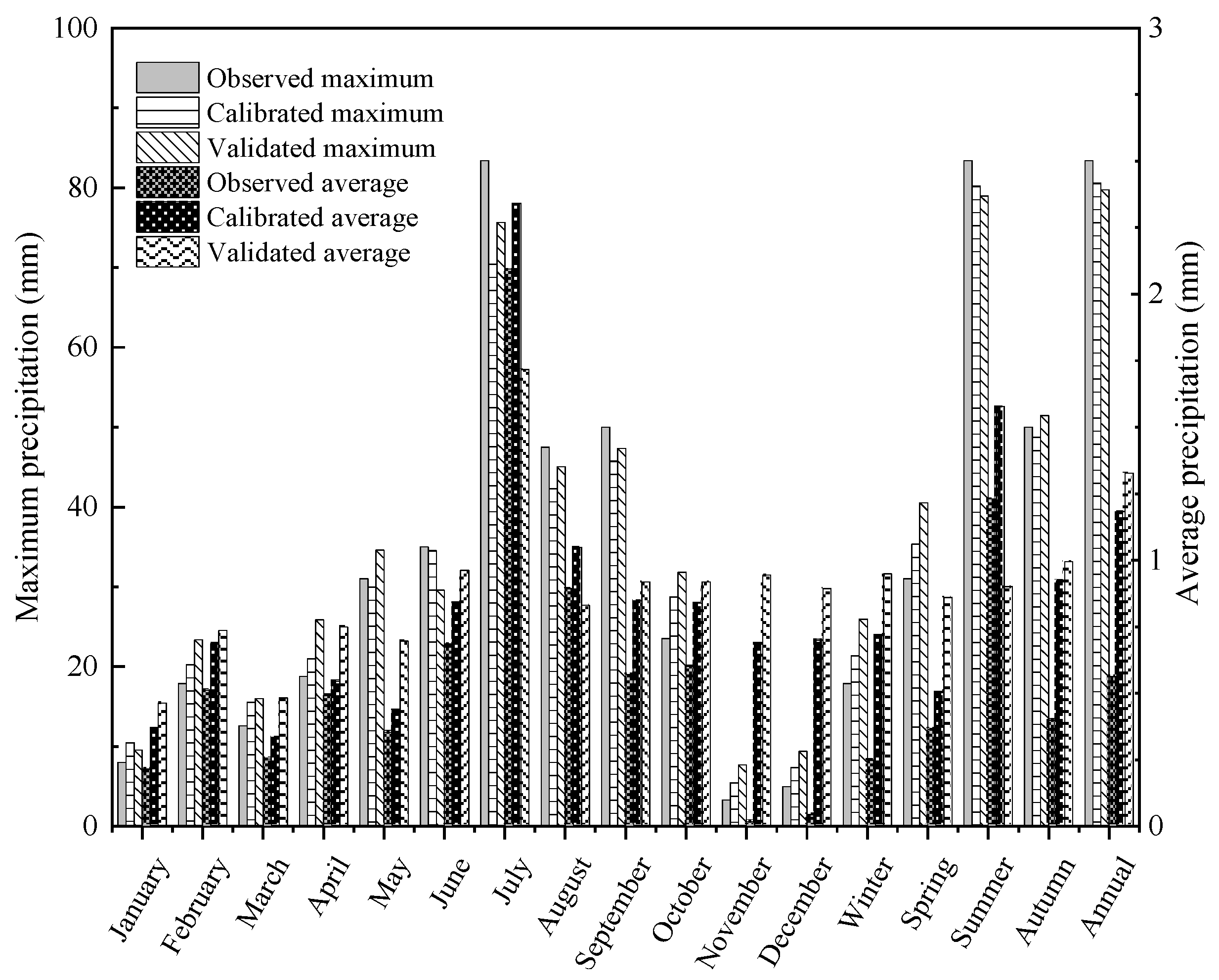
Figure 5 depicts the simulated results for average monthly temperature. It can be seen that these results are in good agreement with field observations. This substantiates the efficacy of the proposed model for temperature simulation and climate projection in the context of temperature change. However, the simulation and projection of precipitation were found slightly challenging for the proposed model. The reason is that during the conditional setup of SDSM for precipitation, the intensity of local precipitation depends on the wet-dry period, which in turn relies on regional predictors like atmospheric pressure and air humidity [48]. This also explains why previous studies [54] show low-performance simulation outputs for precipitation of different regions. Besides the exception of some peaks, the monthly and seasonal mean and maximum simulated precipitation are consistent with the trends in observed data (Figure 6).
3.2. Climate Change Scenarios
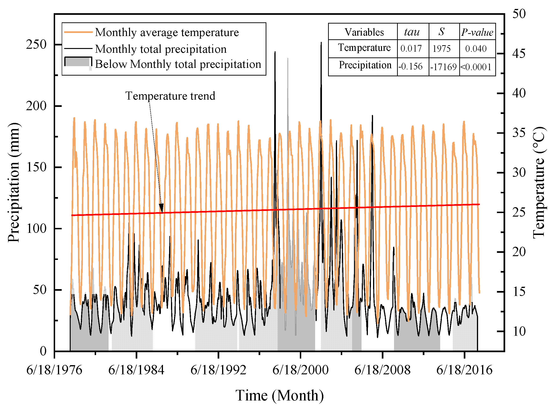
Mann–Kendall’s test results show an increasing trend in the mean monthly temperature and a decreasing trend in the monthly total precipitation. The positive value of S (1975) indicates an upward trend for monthly mean temperature. The positive tau value (0.017) denotes a positive correlation between time and temperature (Figure 7). On the other hand, the negative value of S (−17169) indicates a downward trend for monthly total precipitation, whereas the negative value of tau (−0.156) suggests a negative correlation between time and precipitation. p-values for monthly temperature and precipitation were found smaller than the alpha value (0.050), rejecting the null hypothesis H0 in favor of hypothesis H1. The acceptance of hypothesis H1 is even substantiated by the trend in temperature and precipitation time-series data. Conversely, Kendall’s time series analysis for seasonal temperature rejected the null hypothesis H0 for all seasons (Table 2).
The increase in minimum temperature indices was found superior to 2 °C over the past 40 years. This result is consistent with the work of [55] that conducted research on extreme temperature indices in Pakistan and found that the increase in mean minimum temperature in Punjab province was about 1.9 °C over the past 54 years. However, the increment in maximum temperature indices was less significant than that of minimum temperature since a relatively slight variation was observed. After the 2000s, 2010 was the warmest year, with a maximum temperature of 50 °C around the end of May. In the late 1990s, precipitation reduced to its minimum (83 mm/year) over the previous four decades, and droughts occurred in the region. Moreover, a decrease in air humidity and increased wind speed was observed.
Predicted Temperature and Precipitation
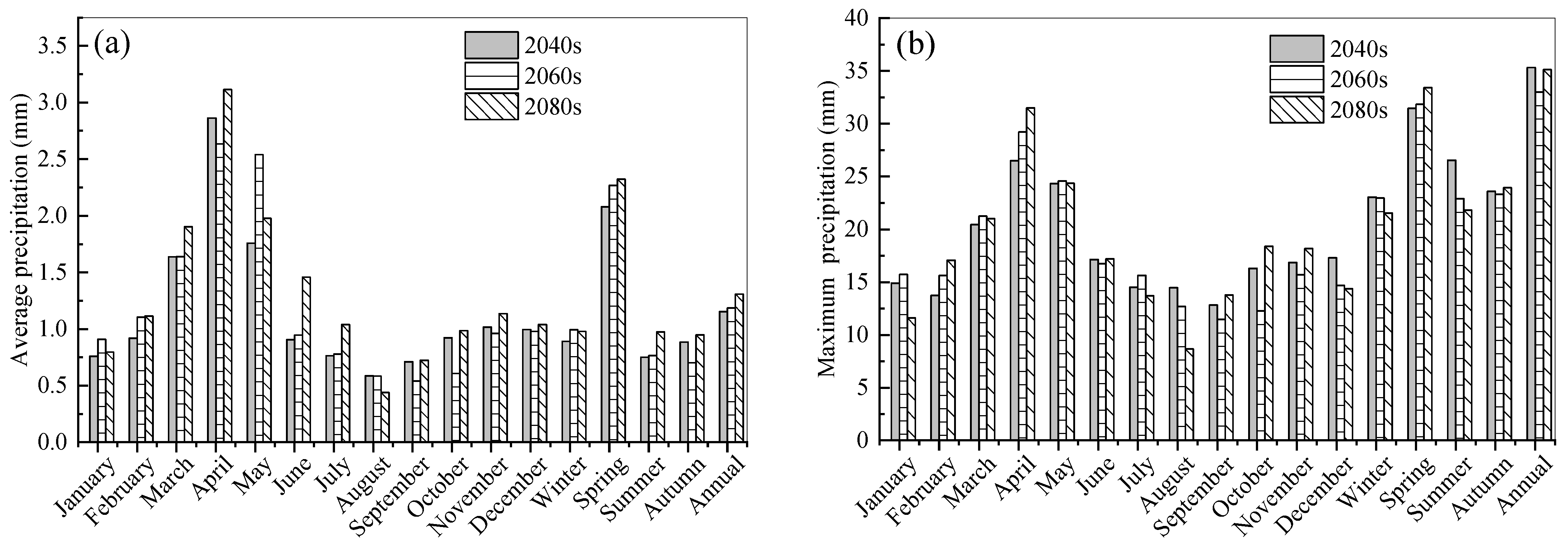
The analysis of GCM predictors reveals an increase in rainfall from March to June and a decline from July to February. The spring season (March–May) shows high precipitation for all three-time scenarios as compared with the other three seasons (winter, summer, and autumn). The predicted maximum monthly rainfall was found to vary between 20.42 and 31.50 mm. Although monthly variations differed from one-time scenario to another, the 2080s scenario was found dominant in monthly mean rainfall in March, April, June, July, October, and November. As depicted in Figure 8, the months of April and May 2060s show maximum precipitation. However, the difference in maximum monthly rainfall is not obvious among all scenarios.
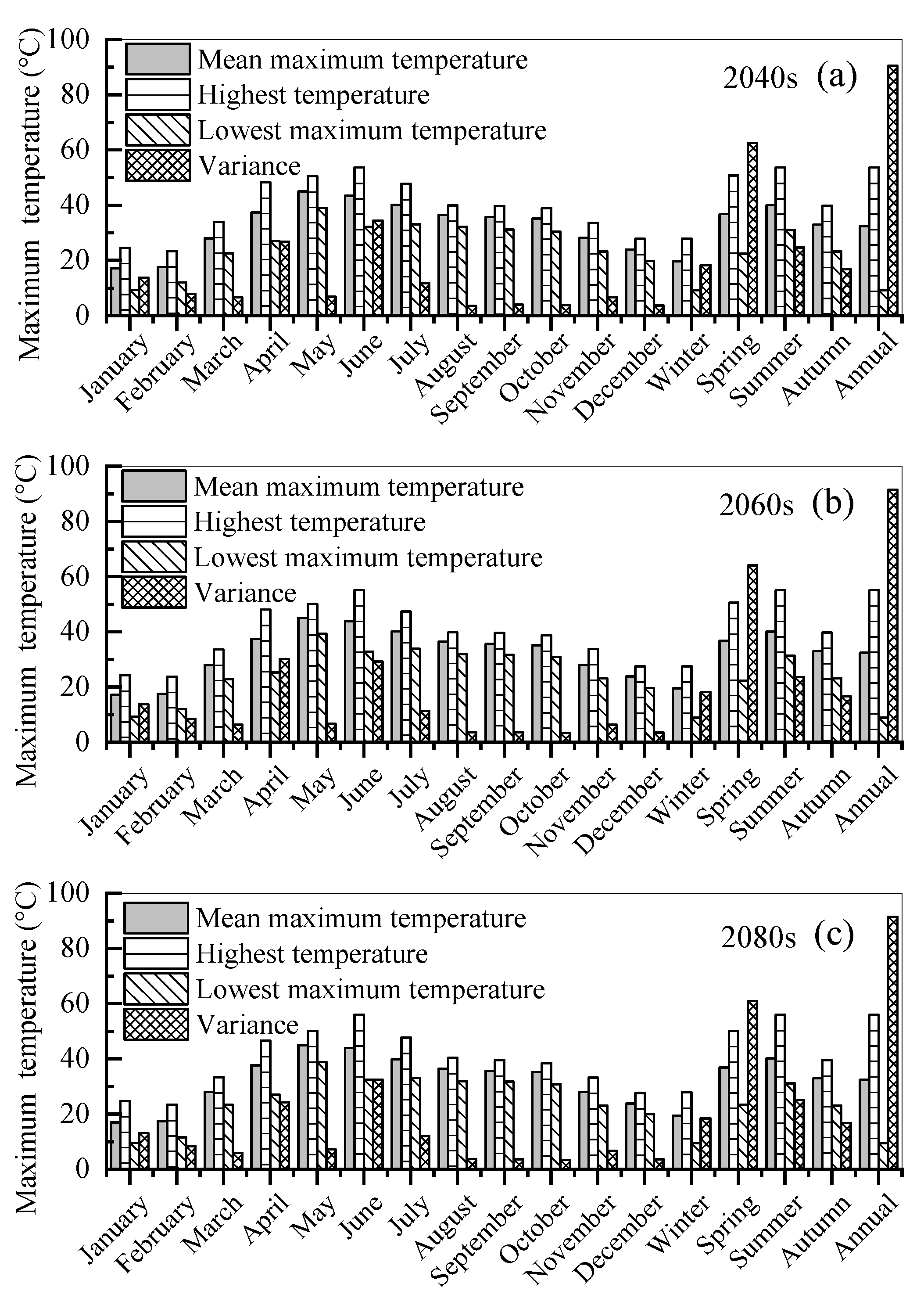
Figure 9 shows a regular increasing trend in projected seasonal and annual maximum temperatures. The results show that the temperature will increase throughout the three scenarios. A probable increase in simulated highest annual temperature is 3.15 °C, 4.25 °C, and 5.93 °C by the 2040s, 2060s, and 2080s, respectively. However, the maximum increment was observed in the summer season, where the mean maximum temperature reaches 39.98 °C, 40.06 °C, and 40.13 °C by the 2040s, 2060s, and 2080s, respectively. June is the warmest month for all three projected scenarios and shows a significant increase in maximum temperature indices. The highest temperature in this month extended to 53.65 °C, 55.04 °C, and 55.91 °C by the 2040s, 2060s, and 2080s, respectively, and lowest maximum temperature extended to 32.21 °C, 32.51 °C, and 32.84 °C by the 2040s, 2060s, and 2080s, respectively.
3.3. Land-Use Land Cover (LULC) Changes
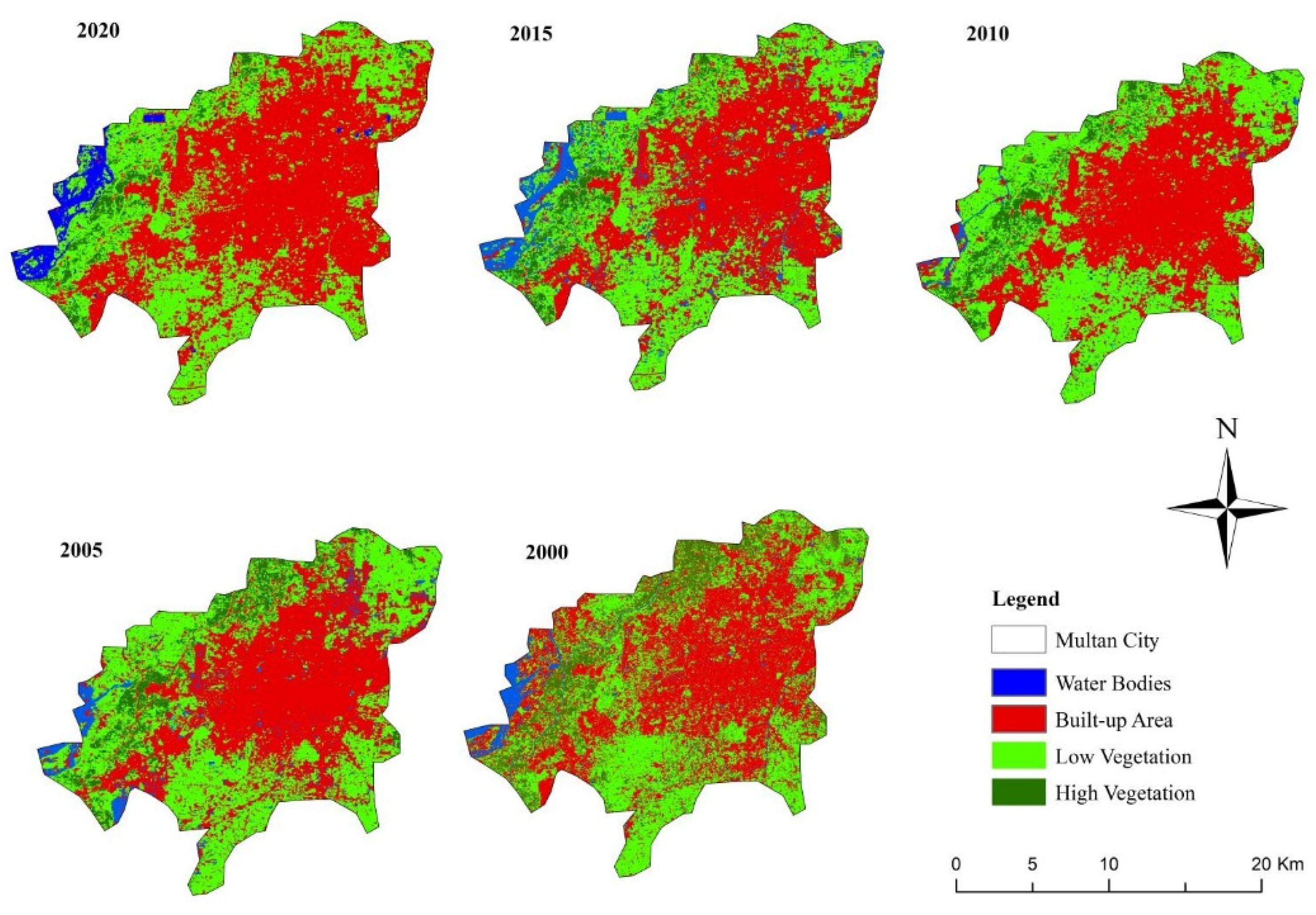
The results of this study expand the work of Manzoor et al. [56] that conducted research on land-use changes in Multan city from 1992 to 2015. They found that the urban land covered which was 1800 ha in 1992, extended by 112.5% and reached 3825.9 ha in 2002. It should be recalled that Multan is the fifth largest city in Pakistan by population. Land-use land cover changes from 2000 to 2020 are shown in Figure 10. It was found that a decade later, i.e., from 2015, a considerable expansion occurred and the urban part increased significantly. The built-up area, that was about 130.03 km2 in 2000, gradually expanded over the last two decades, resulting in an increase of 25.46 km2, to 155.49 km2 in 2020. On the other hand, the low-vegetation cover decreased from 112.94 km2 to 105.4 km2, and the dense vegetation reduced from 31.8 kkm2 to 12.21 km2. An analogous decreasing trend was also observed in the past, with an agricultural area reducing rate of 0.15% between 1992 to 2002 [56]. Soil characteristics and variability in LULC summarized in Table 3 shows that the major land-use classes of the area are residential land, low and high vegetation, unused or bare soil, and water bodies. The water-covered area increased from 11.36 km2 (in 2000) to 15.49 km2 (in 2005) and then decreased to 9.52 km2 in 2010. It expanded again to 21.08 km2 (2015) and then finally reduced to 13.03 km2 (2020) (Figure 10). This happened due to unusual flash floods in the upstream area of the Chenab River basin over the last couple of decades.
3.4. Rainfall-Runoff Simulation and Water Balance
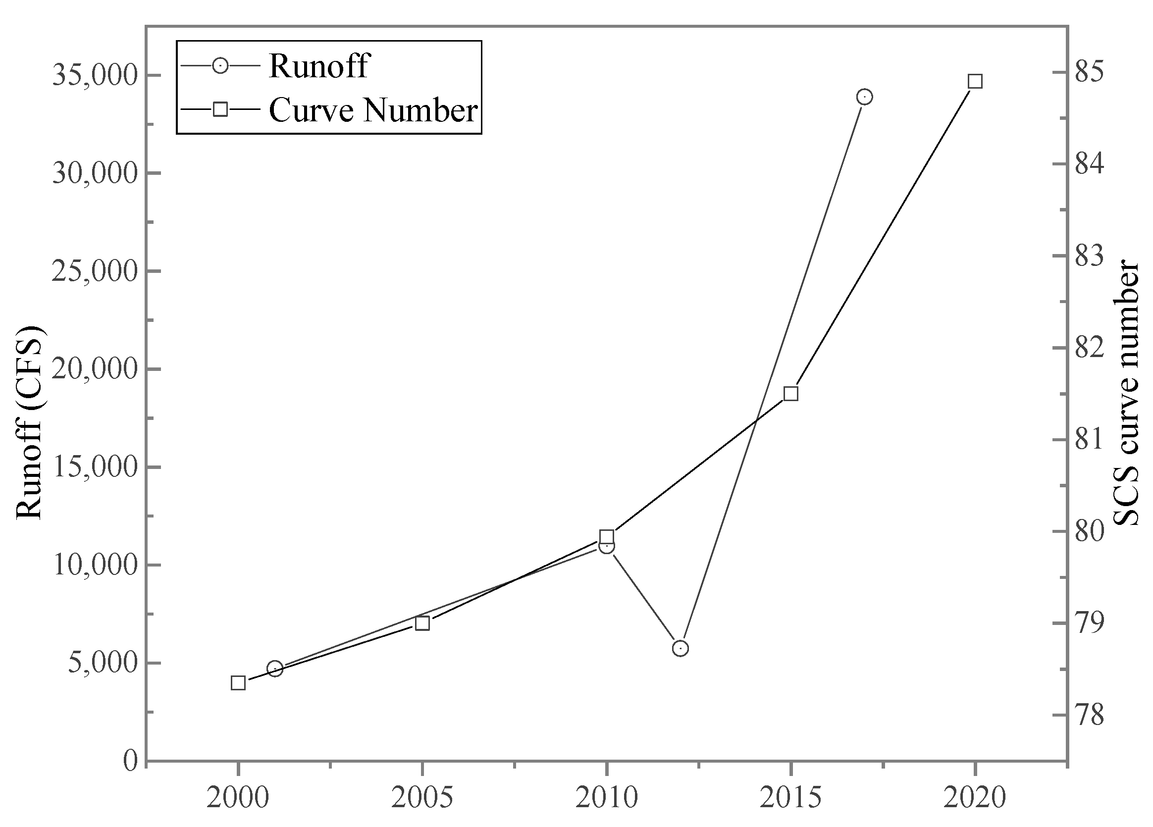
Table 4 summarizes the results of runoff generation for different climate/land-use scenarios. For the four scenarios investigated, the amount of runoff gradually increased from 79 to 85 between the 2000s and 2020s. This substantial increase can be correlated with the rapid urbanization observed in Multan over the last few decades. The SCS curve number was found to have a direct relation with the rate of infiltration and runoff discharge. The correlation between runoff discharge and curve number is shown in Figure 11. It should, however, be noted that no discharge gauges are installed in the study area to calculate the observed runoff and confirm the HEC-HMS simulation performance. Nevertheless, the simulated results are in good agreement with previously published research, which considered the same LULC, meteorological and soil conditions [44]. Moreover, in the first five-year scenario, the outlet point achieved a maximum peak discharge of 133.3 (m3/s) on 25 July 2001. The second five-year scenario reached a maximum discharge of 310.8 m3/s on 08 August 2010. The third and fourth five-year scenarios yielded peak discharges of 162.6 m3/s and 959.6 m3/s on 09 September 2012 and 31 August 2017, respectively. Despite a slight difference in curve number values, similar results were obtained by Rangari et al. [44] for Hyderabad city, where 221.4 mm rainfall transformed into 590.4 m3/s. These results indicate that the increase in urbanization reduces the rate of water infiltration and increases runoff generation, which is one of the main causes of groundwater depletion in the study area.
In summary, using the climatic and Land-use land cover data in HEC-HMS model, it is found that the soil infiltration rate influences overall water balance in the area. Due to the decrease in the rate of infiltration, the groundwater is depleting over time. Extensive urban infrastructure, extreme climate events, and groundwater exploitation also contribute altering the hydrologic cycle. Most of the rainwater is transformed into runoff, while the remaining part evaporates due to arid climate, without recharging the aquifers: causing the depth to water level to drop day by day.
3.5. Coupling Impacts
Both climate and LULC changes play a significant role in water quality and water resources management. The analysis of the combined effect of climate and LULC changes on water resources in the city of Multan indicates three main deleterious impacts. These impacts must be suitably integrated in the water resources management of Multan, particularly in the view of the alarming, predicted climate and LULC changes.
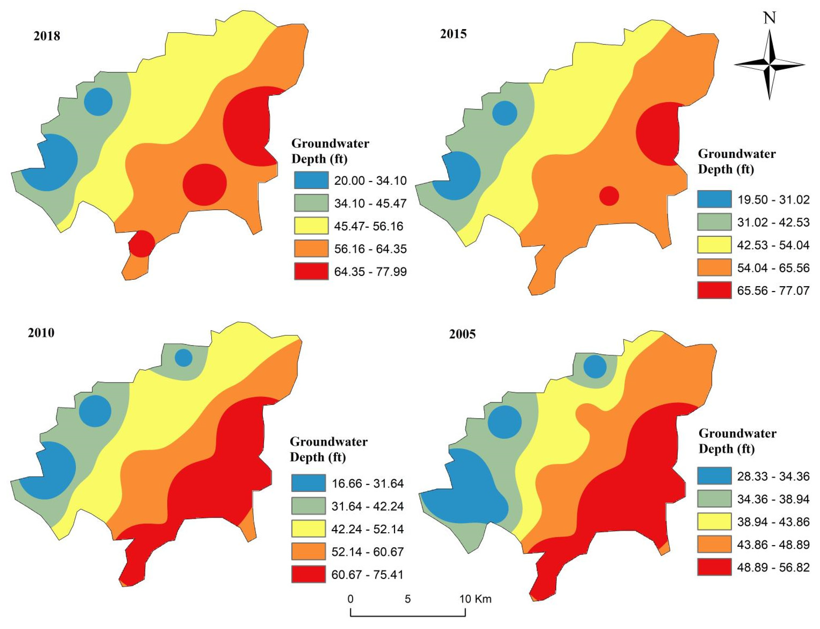
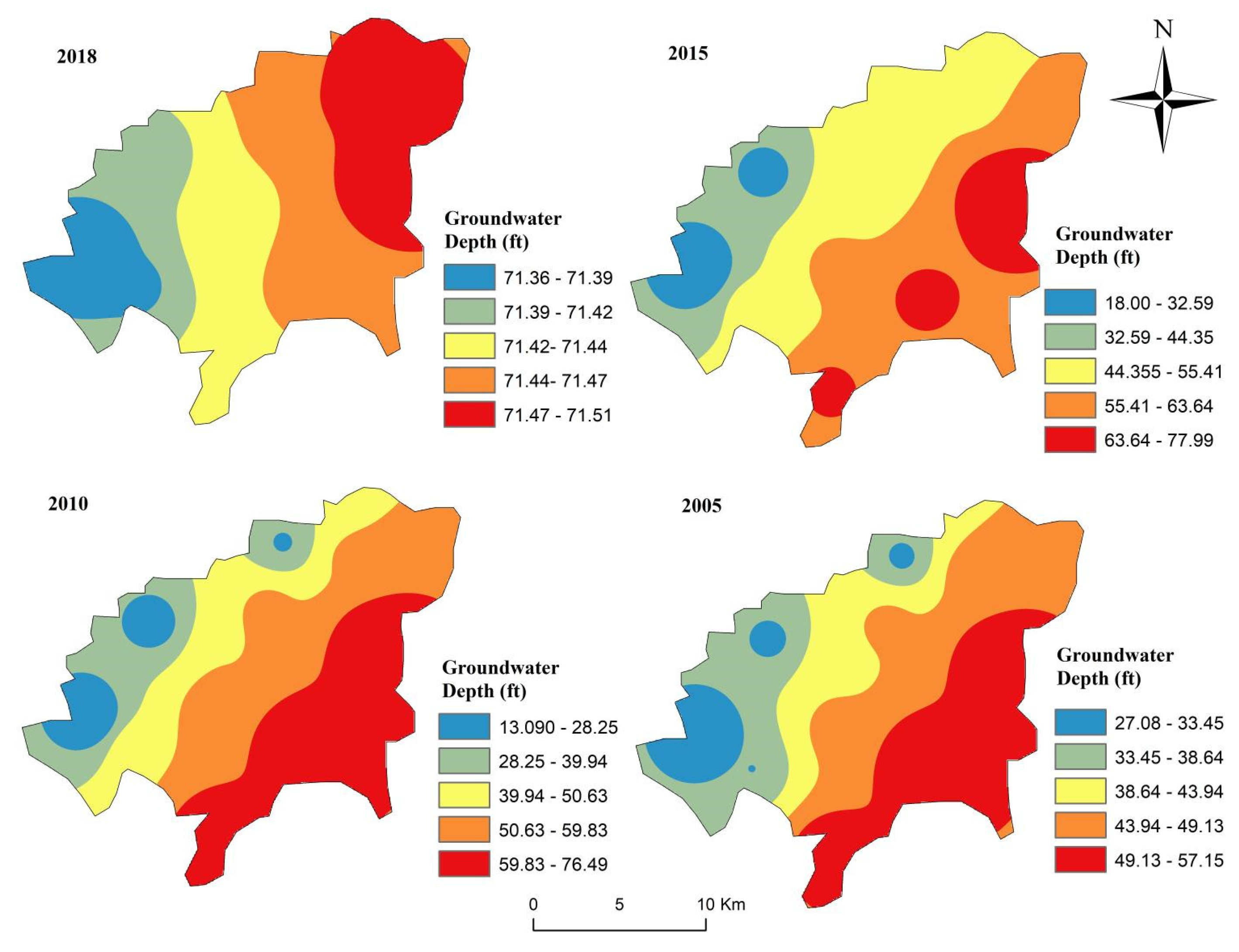
Impact 1: reduction of groundwater resource. It was found that the increase in urbanization comes along with the increase of runoff and a decrease in infiltration rate (natural groundwater recharge). The reduction of groundwater recharge in the region has been exacerbated by the decrease of precipitation which was found to have a decreasing trend, particularly between July and February. The direct consequence of the combination of these mechanisms is that the depth of the water table is also declining with time. According to Young et al. [57], the water table in Multan city dropped by 0.3 m/year. Shallow aquifer accesses are found at a depth of 9.1–12.1 m, but the water extraction for drinking purposes is not fit at this depth due to pollutants (See Impact 2). More generally, over the last few decades, the Punjab plains have been subjected to a significant decline in depth to water level due to the high expansion of groundwater pumping [58]. In Punjab, most of the crops are grown using groundwater, where more than 20% of the agricultural area is irrigated by groundwater and 55% of irrigated land receives groundwater and canal water. Punjab’s groundwater discharge rate exceeds the recharge rate, resulting in a significant decline in groundwater levels in parts of the Punjab province, specifically in lower Bari Doab [57]. Results show that the depth to water table declined approximately by 3~6 m across the study area’s western and eastern parts, respectively, from 2002 to 2014 [57,58]. We speculate that these variations are also influenced by the Monsoon season. In Pakistan, the Monsoon season brings appalling climate conditions, i.e., heavy rainfalls, sudden and flash floods, droughts, sea-level rise, ice retreat, and so forth, influencing the water resources and overall economy. Groundwater table depth was identified between 6 m to 12 m in 2002 and reached almost 9 m to 18 m up to 2014. Variations (rise or fall) in depth to water table for pre-monsoon and post-monsoon are shown in Figure 12 and Figure 13 In the future, modern information technologies, i.e., artificial intelligence [59,60,61,62,63,64], global position system, and remote sensing, should be adopted to investigate the impact on water resources due climate and land-use land variations.
Impact 2: deterioration of water quality. This impact is concomitantly caused by the magnitude of land use and behavior of water cycle. The unplanned and high rate of urbanization in major cities of Pakistan has made it difficult to dispose of solid wastes properly. Multan is among those cities where solid wastes are dumped in the open place or along roadsides without considering water pollution issues. In fact, leachate from waste dumping sites typically possess physicochemical parameters, including color, electrical conductivity (EC), total dissolved solids (TDS), total suspended solids (TSS), biological oxygen demand (BOD), NH3-N, PO4-P, SO42-, and Fe, beyond the WHO threshold [65]. Consequently, the contamination of surface and groundwater in the study area result from the absence of proper and planned disposal sites [65,66]. Infiltration of water containing complex leachate alters water chemistry in shallows aquifers. Further, the Chenab River, which is the primary source of aquifer recharge in the study area, was found to have a significant level of arsenic (As) contamination above the permissible value (WHO standard) in some areas (Figure 14). This situation is alarming for the citizens of Multan that are overly concerned and already complained to the government about the arsenic-contaminated water [37,67] identified that arsenic leaching from phosphogypsum of Pak-Arab Fertilizer Factory is deteriorating water quality and affecting agricultural fields, from where it is moved to the food chain with severe health consequences. Water wells at the Nishter hospital Multan, Cantonment board, Metro Plaza, and Basti Khudadad show the highest level of arsenic concentration (i.e., exceeding 91 ppb) (Figure 14) [58].
Impact 3: depletion of surface water. Significant temperature rise has reduced the air and soil moisture and infiltration rate and has increased the rate of evapotranspiration and atmospheric CO2, resulting in water scarcity in the study area. The growing volume of atmospheric CO2 alters global climate systems, intensifying the hydrological regime with negative consequences on the local water system [68,69]. The historical and projected climate change trends, place Multan as one of the world’s hottest cities. Climate and land-use land cover (LULC) variations have brought surface water resources deterioration and alteration in the water cycle in many other countries around the globe [70,71]. The discrete evaluation of these changes is difficult in the sense that results may vary from one case to another [72,73]. Climate change vulnerability in Pakistan was recognized by the National Water Policy (2018), the Climate Change Act (2017), and the National Climate Change Policy (2012). Water security has been the main concern under climate change, as well as policy measures ranging from developing awareness and additional water conservation storage [74,75].
4. Conclusions
The study presented an investigation on the impacts of climate change-land use variation on water resources of Multan city, Punjab, Pakistan, based on an evaluation of past climate and land-use changes. Multan, having an arid climate, is pronounced part of lower Bari Doab, which lies to the south of Punjab plains. The following conclusions can be summarized:
- (1)
- Results show significant variation in temperature indices, and a regular increment has been observed in minimum temperature indices, which increased significantly over the last 40 years. However, the increment in maximum indices was not regular and varied from year to year. A noticeable decrease in mean annual relative humidity and increase in wind speed were observed over the last four decades;
- (2)
- The urban land extended from 130.03 km2 (45.44%) by 2000 to 155.49 km2 (55.33%) by 2020. Conversely, the dense vegetation decreased from 31.80 km2 (11.11%) by 2000 to 12.2 km2 (4.27%) by 2020, while the light vegetation reduced from 112.94 km2 (39.47%) to 105.40 km2 (36.83%) by 2020. An increase in temperature and urbanization (impervious cover) has reduced the rate of infiltration and increased runoff inflows to the river;
- (3)
- The evaluated results from HEC-HMS revealed that the transition of rainfall into runoff increases with time. On 31 August 2017, the whole catchment basin’s outlet discharge point recorded a maximum surface water runoff of 959.6 m3/s, with 306 mm of rainfall. This indicates that infiltration was minimal and that most of the rainfall was converted to surface runoff. Consequently, the groundwater is depleting rapidly due to an imbalance between discharge and recharge of the groundwater;
- (4)
- The depth of the water table is declining at the rate of 0.2 m per year. Water quantity and water quality are also deteriorating due to unplanned land-use changes and open dumping of domestic and industrial effluents. At some spots, arsenic concentration was found beyond the WHO threshold, creating health issues for the citizens of Multan. Therefore, climate and land-use changes are both deteriorating water distribution and water quality. Moreover, the effects of urbanization were found more prominent and more critical in the study area.
Author Contributions
Conceptualization, M.A.; methodology, M.A. and P.G.A.N.; software, M.A.; validation, M.A. and P.G.A.N.; formal analysis, M.A.; investigation, M.A.; resources, M.A.; data curation, M.A.; writing—original draft preparation, M.A.; writing—review and editing, P.G.A.N.; supervision, Y.W.; project administration, Y.W.; funding acquisition, Y.W. All authors have read and agreed to the published version of the manuscript.
Funding
This research has been supported by the Natural Science foundation of Guangdong Province of China (Grant No. 2022A1515011200), Science and Technology Planning Project of Guangdong Province of China (Grant No. STKJ2021129).
Data Availability Statement
National Centre for Environmental Prediction (NCEP) observed daily predicators and Global Climate Model (GCM) daily predicators were downloaded from the site, Government of Canada (http://climate-scenarios.canada.ca/?page=pred-hadcm3; accessed on 20 September 2020). Historical daily observed maximum and minimum temperature, precipitation, and other climate variables, such as air humidity and wind speed, were collected from Pakistan Metrological Department (PMD). Data for depth to the water table were collected from the Punjab irrigation department. Digital Elevation Model (DEM) and Landsat data were downloaded from the earth explorer, USGS (https://earthexplorer.usgs.gov; accessed on 20 September 2020) site.
Acknowledgments
Financial support and data sources are gratefully acknowledged.
Conflicts of Interest
The authors declare no conflict of interest.
References
- Kundzewicz, Z.W.; Krysanova, V.; Benestad, R.; Hov, Ø.; Piniewski, M.; Otto, I.M. Uncertainty in climate change impacts on water resources. Environ. Sci. Policy 2018, 79, 1–8. [Google Scholar] [CrossRef]
- Liu, Z.; Yang, X.; Hubbard, K.G.; Lin, X. Maize potential yields and yield gaps in the changing climate of northeast China. Glob. Chang. Biol. 2012, 18, 3441–3454. [Google Scholar] [CrossRef]
- Boonwichai, S.; Shrestha, S.; Babel, M.S.; Weesakul, S.; Datta, A. Evaluation of climate change impacts and adaptation strategies on rainfed rice production in Songkhram River Basin, Thailand. Sci. Total Environ. 2019, 652, 189–201. [Google Scholar] [PubMed]
- Lins, H.F.; Cohn, T.A. Stationarity: Wanted dead or alive? J. Am. Water Resour. Assoc. 2011, 47, 475–480. [Google Scholar]
- Lin, S.S.; Zhen, S.L.; Zhou, A.; Xu, Y.S. Approach based on TOPSIS and Monte Carlo simulation methods to evaluate lake eutrophication levels. Water Res. 2020, 187, 116437. [Google Scholar] [CrossRef]
- Lin, S.S.; Shen, S.L.; Zhou, A.; Lyu, H.-M. Sustainable development and environmental restoration in Lake Erhai, China. J. Clean. Prod. 2020, 258, 120758. [Google Scholar] [CrossRef]
- Lin, S.S.; Shen, S.L.; Zhang, N.; Zhou, A. Modelling the performance of EPB shield tunnelling using machine and deep learning algorithms. Geosci. Front. 2021, 12, 101177. [Google Scholar] [CrossRef]
- Lin, S.S.; Shen, S.L.; Lyu, H.M.; Zhou, A. Assessment and management of lake eutrophication: A case study in Lake Erhai, China. Sci. Total Environ. 2021, 751, 141618. [Google Scholar] [CrossRef]
- Lyu, H.M.; Sun, W.J.; Shen, S.L.; Arulrajah, A. Flood risk assessment in metro systems of mega-cities using a GIS-based modeling approach. Sci. Total Environ. 2018, 626, 1012–1025. [Google Scholar] [CrossRef]
- Lyu, H.M.; Zhou, A.N.; Yang, J. Perspectives for flood risk assessment and management for mega-city metro system. Tunn. Undergr. Space Technol. 2019, 84, 31–44. [Google Scholar] [CrossRef]
- Lyu, H.M.; Zhou, A.; Yang, J. Risk assessment of mega-city infrastructures related to land subsidence using improved trapezoidal FAHP. Sci. Total Environ. 2020, 717, 135310. [Google Scholar] [CrossRef] [PubMed]
- Lyu, H.M.; Zhou, W.H.; Shen, S.L.; Zhou, A. Inundation risk assessment of metro system using AHP and TFN-AHP in Shenzhen. Sustain. Cities Soc. 2020, 56, 102103. [Google Scholar] [CrossRef]
- Lyu, H.M.; Sun, W.J.; Shen, S.L.; Zhou, A. Risk assessment using a new consulting process in fuzzy AHP. J. Constr. Eng. Manag. ASCE 2020, 146, 04019112. [Google Scholar]
- Lyu, H.M.; Zhou, A.N.; Zhou, W.H. Flood risk assessment of metro systems in a subsiding environment using the interval FAHP-FCA approach. Sustain. Cities Soc. 2019, 50, 101682. [Google Scholar] [CrossRef]
- Lyu, H.M.; Chou, A. The development of IFN-SPA: A new risk assessment method of urban water quality and its application in Shanghai. J. Clean. Prod. 2021, 282, 124542. [Google Scholar]
- Lyu, H.M.; Shen, S.L.; Wu, Y.X.; Zhou, A. Calculation of groundwater head distribution with a close barrier during excavation dewatering in confined aquifer. Geosci. Front. 2021, 12, 791–803. [Google Scholar] [CrossRef]
- Poorsepahy-Samian, H.; Espanmanesh, V.; Zahraie, B. Improved inflow modeling in stochastic dual dynamic programming. J. Water Resour. Plan. Manag. 2016, 142, 04016065. [Google Scholar]
- Matheussen, B.; Kirschbaum, R.L.; Goodman, I.A.; O’Donnell, G.M.; Lettenmaier, D.P. Effects of land cover change on streamflow in the interior Columbia River Basin (USA and Canada). Hydrol. Processes 2000, 14, 867–885. [Google Scholar] [CrossRef]
- Lyu, H.M.; Shen, S.L.; Zhou, A.; Yin, Z.Y. Assessment of safety status of shield tunnelling using operational parameters with enhanced SPA. Tunn. Undergr. Space Technol. 2022, 123, 104428. [Google Scholar] [CrossRef]
- Shen, S.L.; Atangana Njock, P.G.; Zhou, A. Dynamic prediction of jet grouted column diameter in soft soil using Bi-LSTM deep learning. Acta Geotech. 2021, 16, 303–315. [Google Scholar] [CrossRef]
- Lin, S.S.; Zhang, N.; Zhou, A. Risk evaluation of excavation based on fuzzy decision-making model. Autom. Constr. 2022, 136, 104143. [Google Scholar] [CrossRef]
- Wu, Y.X.; Lyu, H.M. Analyses of leakage effect of waterproof curtain during excavation dewatering. J. Hydrol. 2020, 583, 124582. [Google Scholar] [CrossRef]
- Zhang, N.; Zhou, A.; Jin, Y.F. Application of LSTM approach for modelling stress-strain behavior of soil. Appl. Soft Comput. 2021, 100, 106959. [Google Scholar] [CrossRef]
- Deng, J.L.; Shen, S.L.; Xu, Y.S. Investigation into pluvial flooding hazards caused by heavy rain and protection measures in Shanghai, China. Nat. Hazards 2016, 83, 1301–1320. [Google Scholar] [CrossRef]
- Weng, Q. Modeling urban growth effects on surface runoff with the integration of remote sensing and GIS. Environ. Manag. 2001, 28, 737–748. [Google Scholar] [CrossRef]
- Lin, S.S.; Shen, S.L.; Zhang, N.; Zhou, A. An extended TODIM-based model for evaluating risks of excavation system. Acta Geotech. 2022, 17, 1053–1069. [Google Scholar] [CrossRef]
- Kundzewicz, Z.W.; Stakhiv, E.Z. Are climate models “ready for prime time” in water resources management applications, or is more research needed? Hydrol. Sci. J. 2010, 55, 1085–1089. [Google Scholar] [CrossRef]
- Moglen, G.E.; Rios Vidal, G.E. Climate change and storm water infrastructure in the mid-Atlantic region: Design mismatch coming? J. Hydrol. Eng. 2014, 19, 04014026. [Google Scholar] [CrossRef]
- Wu, Y.X.; Lu, H.M.; Zhou, A. A three-dimensional fluid-solid coupled numerical modeling of the barrier leakage below the excavation surface due to dewatering. Hydrogeol. J. 2020, 28, 1449–1463. [Google Scholar] [CrossRef]
- Slingo, J.; Palmer, T. Uncertainty in weather and climate prediction. Philosophical Transactions of the Royal Society A: Mathematical. Phys. Eng. Sci. 2011, 369, 4751–4767. [Google Scholar]
- Wu, H.L.; Cheng, W.C.; Lin, M.Y.; Arulrajah, A. Variation of hydro-environment during past four decades with underground sponge city planning to control flash floods in Wuhan, China: An overview. Undergr. Space 2020, 5, 184–198. [Google Scholar] [CrossRef]
- Murphy, J. Predictions of climate change over Europe using statistical and dynamical downscaling techniques. Int. J. Climatol. 2000, 20, 489–501. [Google Scholar] [CrossRef]
- Zhang, N.; Zhou, A.; Pan, Y.T. Measurement and prediction of tunnelling-induced ground settlement in karst region by using expanding deep learning. Measurement 2021, 183, 109700. [Google Scholar] [CrossRef]
- Greenman, D.W.; Bennett, G.D.; Swarzenski, W.V. Ground-Water Hydrology of the Punjab, West Pakistan, with Emphasis on Problems Caused by Canal Irrigation; US Government Printing Office: Washington, DC, USA, 1967. [Google Scholar]
- Hasan, M.; Shang, Y.; Akhter, G.; Jin, W. Application of VES and ERT for delineation of fresh-saline interface in alluvial aquifers of Lower Bari Doab, Pakistan. J. Appl. Geophys. 2019, 164, 200–213. [Google Scholar] [CrossRef]
- Wu, H.N.; Shen, S.L.; Chen, R.P.; Zhou, A. Three-dimensional numerical modelling on localised leakage in segmental lining of shield tunnels. Comput. Geotech. 2020, 122, 103549. [Google Scholar] [CrossRef]
- Murtaza, G.; Habib, R.; Shan, A.; Sardar, K.; Rasool, F.; Javeed, T. Municipal solid waste and its relation with groundwater contamination in Multan, Pakistan. IJAR 2017, 3, 434–441. [Google Scholar]
- Young, W.J.; Anwar, A.; Bhatti, T.; Borgomeo, E.; Davies, S.; Garthwaite, W.R., III; Gilmont, E.M.; Leb, C.; Lytton, L.; Makin, I. Pakistan: Getting More from Water; World Bank: Washington, DC, USA, 2019. [Google Scholar]
- Lee, J.; Pak, G.; Yoo, C.; Kim, S.; Yoon, J. Effects of land use change and water reuse options on urban water cycle. J. Environ. Sci. 2010, 22, 923–928. [Google Scholar] [CrossRef]
- Djokic, D.; Maidment, D.R. Terrain analysis for urban stormwater modelling. Hydrol. Process. 1991, 5, 115–124. [Google Scholar] [CrossRef]
- Parece, T.E.; Campbell, J.B. Delineating Drainage Networks in Urban Areas. In Proceedings of the ASPRS 2014 Annual Conference, Louisville, KY, USA, 23–28 March 2014; pp. 23–27. [Google Scholar]
- DeFries, R.; Eshleman, K.N. Land-use change and hydrologic processes: A major focus for the future. Hydrol. Process. 2004, 18, 2183–2186. [Google Scholar] [CrossRef]
- Foster, S.; Morris, B.; Lawrence, A. Effects of Urbanization on Groundwater Recharge. Groundwater Problems in Urban Areas. In Proceedings of the International Conference Organized by the Institution of Civil Engineers, London, UK, 2–3 June 1993; Thomas Telford Publishing: London, UK, 1994; pp. 43–63. [Google Scholar]
- Marsalek, J.; Cisneros, B.J.; Karamouz, M.; Malmquist, P.-A.; Goldenfum, J.A.; Chocat, B. Urban Water Cycle Processes and Interactions: Urban Water Series-UNESCO-IHP; CRC Press: Boca Raton, FL, USA, 2008. [Google Scholar]
- DeBusk, K.M.; Hunt, W.F.; Hatch, U.; Sydorovych, O. Watershed retrofit and management evaluation for urban stormwater management systems in North Carolina. J. Contemp. Water Res. Educ. 2010, 146, 64–74. [Google Scholar] [CrossRef] [Green Version]
- Civco, D.L.; Hurd, J.D.; Wilson, E.H.; Arnold, C.L.; Prisloe, M.P., Jr. Quantifying and describing urbanizing landscapes in the Northeast United States. Photogramm. Eng. Remote Sens. 2002, 68, 1083–1090. [Google Scholar]
- Slonecker, E.T.; Jennings, D.B.; Garofalo, D. Remote sensing of impervious surfaces: A review. Remote Sens. Rev. 2001, 20, 227–255. [Google Scholar] [CrossRef]
- Wilby, R.L.; Charles, S.P.; Zorita, E.; Timbal, B.; Whetton, P.; Mearns, L.O. Guidelines for Use of Climate Scenarios Developed from Statistical Downscaling Methods. Supporting Material of the Intergovernmental Panel on Climate Change, Available from the DDC of IPCC TGCIA. 2004. Available online: https://www.researchgate.net/publication/200472164 (accessed on 27 April 2022).
- Wilby, R.L.; Hay, L.E.; Leavesley, G.H. A comparison of downscaled and raw GCM output: Implications for climate change scenarios in the San Juan River basin, Colorado. J. Hydrol. 1999, 225, 67–91. [Google Scholar] [CrossRef]
- Wilby, R.L.; Dawson, C.W.; Barrow, E.M. SDSM—A decision support tool for the assessment of regional climate change impacts. Environ. Model. Softw. 2002, 17, 145–157. [Google Scholar] [CrossRef]
- Mekonnen, D.F.; Duan, Z.; Rientjes, T.; Disse, M. Analysis of combined and isolated effects of land-use and land-cover changes and climate change on the upper Blue Nile River basin’s streamflow. Hydrol. Earth Syst. Sci. 2018, 22, 6187–6207. [Google Scholar] [CrossRef] [Green Version]
- Zhang, J.; Li, Q.; Gong, H.; Li, X.; Song, L.; Huang, J. Hydrologic Information Extraction Based on Arc Hydro Tool and DEM. In Proceedings of the International Conference on Challenges in Environmental Science and Computer Engineering, Wuhan, China, 6–7 March 2010; pp. 503–506. [Google Scholar]
- Rangari, V.A.; Sridhar, V.; Umamahesh, N.; Patel, A.K. Rainfall Runoff Modelling of Urban Area Using HEC-HMS: A Case Study of Hyderabad City. In Advances in Water Resources Engineering and Management; Springer: New York, NY, USA, 2020; pp. 113–125. [Google Scholar]
- Koukidis, E.N.; Berg, A.A. Sensitivity of the Statistical DownScaling Model (SDSM) to reanalysis products. Atmos. Ocean 2009, 47, 1–18. [Google Scholar] [CrossRef]
- Sajjad, H.; Ghaffar, A. Observed, simulated and projected extreme climate indices over Pakistan in changing climate. Theor. Appl. Climatol. 2019, 137, 255–281. [Google Scholar] [CrossRef]
- Manzoor, S.A.; Malik, A.; Zubair, M.; Griffiths, G.; Lukac, M. Linking social perception and provision of ecosystem services in a sprawling urban landscape: A case study of Multan, Pakistan. Sustainability 2019, 11, 654. [Google Scholar] [CrossRef] [Green Version]
- Wu, Y.X.; Chen, S.L.; Yuan, D.J. Characteristics of dewatering induced drawdown curve under blocking effect of retaining wall in aquifer. J. Hydrol. 2016, 539, 554–566. [Google Scholar] [CrossRef]
- Soncini, A.; Bocchiola, D.; Rosso, R.; Meucci, S.; Pala, F.; Valé, G. Water and Sanitation in Multan, Pakistan. In Sustainable Social, Economic and Environmental Revitalization in Multan City; Springer: New York, NY, USA, 2014; pp. 149–162. [Google Scholar]
- Elbaz, K.; Yan, T.; Zhou, A. Deep learning analysis for energy consumption of shield tunneling machine drive system. Tunn. Undergr. Space Technol. 2022, 123, 104405. [Google Scholar] [CrossRef]
- Shen, S.L.; Vhou, A.; Lu, L.-H.; Li, G.; Hu, B.-B. Automatic control of groundwater balance to combat dewatering during construction of a metro system. Autom. Constr. 2021, 123, 103536. [Google Scholar] [CrossRef]
- Shen, S.L.; Elbaz, K.; Shaban, W.M.; Zhou, A. Real-time prediction of shield moving trajectory during tunnelling. Acta Geotech. 2022, 17, 1533–1549. [Google Scholar] [CrossRef]
- Lin, S.S.; Zhang, N.; Zhou, A. Time-series prediction of shield movement performance during tunneling based on hybrid model. Tunn. Undergr. Space Technol. 2022, 119, 104245. [Google Scholar] [CrossRef]
- Wu, Y.X.; Lyu, H.M.; Han, J.; Shen, S.L. Dewatering-induced building settlement around a deep excavation in soft deposit in Tianjin, China. J. Geotech. Geoenviron. Eng. ASCE 2019, 145, 05019003. [Google Scholar] [CrossRef]
- Shen, S.L.; Zhang, N.; Zhou, A.; Yin, Z.Y. Enhancement of neural networks with an alternative activation function tanhLU. Expert Syst. Appl. 2022, 199, 117181. [Google Scholar] [CrossRef]
- Karim, S. Impacts of solid waste leachate on groundwater and surface water quality. J. Chem. Soc. Pak. 2010, 32, 606–612. [Google Scholar]
- Manan, A. E. coli Affecting Groundwater Quality; The Daily Times: Lahore, Pakistan, 2008. [Google Scholar]
- Tariq, S.R.; Shaheen, N.; Khalique, A.; Shah, M.H. Distribution, correlation, and source apportionment of selected metals in tannery effluents, related soils, and groundwater—A case study from Multan, Pakistan. Environ. Monit. Assess. 2010, 166, 303–312. [Google Scholar] [CrossRef]
- Eamus, D. The interaction of rising CO2 and temperatures with water use efficiency. Plant Cell Environ. 1991, 14, 843–852. [Google Scholar] [CrossRef]
- Owensby, C.; Ham, J.; Knapp, A.; Bremer, D.; Auen, L. Water vapour fluxes and their impact under elevated CO2 in a C4-tallgrass prairie. Glob. Chang. Biol. 1997, 3, 189–195. [Google Scholar] [CrossRef] [Green Version]
- Dai, X.; Zhou, Y.; Ma, W.; Zhou, L. Influence of spatial variation in land-use patterns and topography on water quality of the rivers inflowing to Fuxian Lake, a large deep lake in the plateau of southwestern China. Ecol. Eng. 2017, 99, 417–428. [Google Scholar] [CrossRef]
- Wang, R.; Kalin, L. Combined and synergistic effects of climate change and urbanization on water quality in the Wolf Bay watershed, southern Alabama. J. Environ. Sci. 2018, 64, 107–121. [Google Scholar] [CrossRef] [PubMed]
- Ranjan, S.P.; Kazama, S.; Sawamoto, M. Effects of climate and land use changes on groundwater resources in coastal aquifers. J. Environ. Manag. 2006, 80, 25–35. [Google Scholar] [CrossRef] [PubMed] [Green Version]
- Tu, J. Combined impact of climate and land use changes on streamflow and water quality in eastern Massachusetts, USA. J. Hydrol. 2009, 379, 268–283. [Google Scholar] [CrossRef]
- Lyu, H.M.; Shen, S.L.; Yang, J.; Yin, Z.Y. Inundation analysis of metro systems with the storm water management model incorporated into a geographical information system: A case study in Shanghai. Hydrol. Earth Syst. Sci. 2019, 23, 4293–4307. [Google Scholar] [CrossRef] [Green Version]
- Xu, Y.S.; Yan, X.X.; Shen, S.L.; Zhou, A. Experimental investigation on the blocking of groundwater seepage from a waterproof curtain during pumped dewatering in an excavation. Hydrogeol. J. 2019, 27, 2659–2672. [Google Scholar] [CrossRef]
Figure 1.
Map of the research area, including sub-catchments.

Figure 2.
Natural hydrologic system of drainage point, drainage line, fil, adjoining catchment, and catchment polygons.
Figure 2.
Natural hydrologic system of drainage point, drainage line, fil, adjoining catchment, and catchment polygons.

Figure 3.
Schematic methodological framework.

Figure 4.
Schematic diagram for the HEC-HMS model setup.

Figure 5.
SDSM calibration and validation using NCEP and GCMs predictors, respectively, for monthly mean temperature: (a) calibration and (b) validation.
Figure 5.
SDSM calibration and validation using NCEP and GCMs predictors, respectively, for monthly mean temperature: (a) calibration and (b) validation.

Figure 6.
SDSM calibration and validation using NCEP and GCMs; For mean and maximum precipitation.

Figure 7.
Climograph along with Mann–Kendall’s test results showing trends for monthly average temperature and monthly total precipitation.
Figure 7.
Climograph along with Mann–Kendall’s test results showing trends for monthly average temperature and monthly total precipitation.

Figure 8.
The projected (a) mean precipitation and (b) maximum precipitation for the 2040s, 2060s, and 2080s scenarios.
Figure 8.
The projected (a) mean precipitation and (b) maximum precipitation for the 2040s, 2060s, and 2080s scenarios.

Figure 9.
Statics of maximum temperature indices: (a) 2040s, (b) 2060s, and (c) 2080s.

Figure 10.
Land-use land cover changes from 2000 to 2020 of the study area.

Figure 11.
Relation between SCS curve number and peak runoff discharge.

Figure 12.
Spatial variability in pre-monsoon water table depth from 2005 to 2018.

Figure 13.
Spatial variability in post-monsoon water table depth from 2005 to 2018.

Figure 14.
Spatial variability in arsenic concentration.


Table 1.
Selected predictors for maximum and minimum temperature and precipitation.
| Predictor Name | Code | Partial Correlation (Partialr) |
|---|---|---|
| Tmax (Predictand) | ||
| Mean temperature | Temp | 0.589 |
| 500 hPa geopotential height | p500 | 0.424 |
| 850 hPa vorticity | p8_z | 0.257 |
| 850 hPa divergence | p8_zh | 0.172 |
| 850 hPa geopotential height | p850 | 0.177 |
| Relative humidity at 500 hPa | r500 | 0.142 |
| Tmin (Predictand) | ||
| Mean temperature | Temp | 0.672 |
| 500 hPa geopotential height | p500 | 0.521 |
| 850 hPa vorticity | p8_z | 0.252 |
| 500 hPa vorticity | p5_z | 0.206 |
| 850 hPa meridional velocity | p8_v | 0.228 |
| Near surface specific humidity | Shum | 0.170 |
| Precipitation (Predictand) | ||
| Near surface specific humidity | Shum | 0.194 |
| 850 hPa divergence | p8_zh | 0.143 |
| Surface divergence | p_zh | 0.101 |
| Mean temperature | Temp | 0.073 |
| Surface wind direction | P_th | 0.028 |
Table 2.
Summary statistics for seasonal temperature and precipitation along with Mann–Kendall’s test results.
Table 2.
Summary statistics for seasonal temperature and precipitation along with Mann–Kendall’s test results.
| Seasonal Mean for Max Temperature (°C) | Mann–Kendall’s Test Results | ||||||||
|---|---|---|---|---|---|---|---|---|---|
| Season | Minimum | Maximum | Mean | Std. Deviation | Kendall’s Tau | S | p-Value | Alpha | Interpretation |
| Summer | 37.50 | 41.10 | 39.521 | 0.788 | −0.328 | −242.000 | 0.004 | 0.050 | Reject H0 |
| Winter | 20.66 | 23.96 | 22.174 | 0.868 | −0.263 | −193.000 | 0.020 | 0.050 | Reject H0 |
| Spring | 32.13 | 38.20 | 35.135 | 1.577 | 0.130 | 96.000 | 0.040 | 0.050 | Reject H0 |
| Autumn | 30.46 | 34.46 | 33.091 | 0.786 | −0.301 | −222.000 | 0.007 | 0.050 | Reject H0 |
| Seasonal total precipitant (mm) | Mann–Kendall’s test results | ||||||||
| Summer | 3.200 | 277.400 | 106.426 | 63.816 | 0.069 | 51.000 | 0.545 | 0.050 | Accept H0 |
| Winter | 0.000 | 115.000 | 29.405 | 27.649 | 0.011 | 8.000 | 0.933 | 0.050 | Accept H0 |
| Spring | 0.600 | 125.600 | 46.608 | 28.999 | −0.050 | −37.000 | 0.663 | 0.050 | Accept H0 |
| Autumn | 0.000 | 214.700 | 33.172 | 49.709 | 0.126 | 93.000 | 0.266 | 0.050 | Accept H0 |
Table 3.
Soil characteristics and LULC changes from 2000 to 2020.
| Symbol | HWSD-Soil Group | Soil Type | Area | Texture | Topsoil | pH Water Topsoil | pH Water Subsoil | |||
|---|---|---|---|---|---|---|---|---|---|---|
| (km²) | (%) | Sand (%) | Silt (%) | Clay (%) | ||||||
| Yh | Haplic Yermosols | Sandy loam | 280 | 97.90 | Medium | 50.4 | 29 | 20.6 | 6.6 | 6.8 |
| Jc | Calcaric Fluvisols | Loam | 6 | 2.09 | Medium | 39.6 | 39.9 | 20.6 | 8 | 8.1 |
| Years | Build-up area | Light vegetation | Dense vegetation | Water | Curve Number (CN) | |||||
| (km2) | (%) | (km2) | (%) | (km2) | (%) | (km2) | (%) | |||
| 2000 | 130.03 | 45.44 | 112.94 | 39.47 | 31.8 | 11.11 | 11.36 | 3.97 | 78.35 | |
| 2005 | 131.08 | 45.8 | 118.42 | 41.38 | 21.15 | 7.39 | 15.49 | 5.41 | 79 | |
| 2010 | 135.05 | 47.19 | 121.5 | 42.46 | 20.06 | 7 | 9.52 | 3.33 | 79.94 | |
| 2015 | 140.91 | 49.24 | 108.89 | 38 | 15.25 | 5.33 | 21.08 | 7.36 | 81.50 | |
| 2020 | 155.49 | 54.33 | 105.4 | 36.83 | 12.21 | 4.27 | 13.03 | 4.55 | 84.9 | |
Table 4.
Runoff generation for different climate/land-use scenarios.
| Scenario | Peak Runoff Date | Rainfall (mm) | Curve Number (CN) | Volume (INC) | Simulated Runoff (m3/s) |
|---|---|---|---|---|---|
| 2000–2005 | 25 July 2001 | 83.4 | 79 | 2.02 | 133.3 |
| 2006–2010 | 8 August 2010 | 120 | 79.94 | 2.52 | 310.8 |
| 2011–2015 | 9 September 2012 | 76.5 | 81.50 | 3.23 | 162.6 |
| 2016–2020 | 31 August 2017 | 300 | 84.9 | 11.85 | 959.6 |
Publisher’s Note: MDPI stays neutral with regard to jurisdictional claims in published maps and institutional affiliations. |
© 2022 by the authors. Licensee MDPI, Basel, Switzerland. This article is an open access article distributed under the terms and conditions of the Creative Commons Attribution (CC BY) license (https://creativecommons.org/licenses/by/4.0/).
Share and Cite
MDPI and ACS Style
Abbas, M.; Atangana Njock, P.G.; Wang, Y. Influence of Climate Change and Land-Use Alteration on Water Resources in Multan, Pakistan. Appl. Sci. 2022, 12, 5210. https://0-doi-org.brum.beds.ac.uk/10.3390/app12105210
AMA Style
Abbas M, Atangana Njock PG, Wang Y. Influence of Climate Change and Land-Use Alteration on Water Resources in Multan, Pakistan. Applied Sciences. 2022; 12(10):5210. https://0-doi-org.brum.beds.ac.uk/10.3390/app12105210
Chicago/Turabian StyleAbbas, Mohsin, Pierre Guy Atangana Njock, and Yanning Wang. 2022. "Influence of Climate Change and Land-Use Alteration on Water Resources in Multan, Pakistan" Applied Sciences 12, no. 10: 5210. https://0-doi-org.brum.beds.ac.uk/10.3390/app12105210
Note that from the first issue of 2016, this journal uses article numbers instead of page numbers. See further details here.