An Effective AUSM-Type Scheme for Both Cases of Low Mach Number and High Mach Number

Abstract

A new scheme called AUSMAS (Advection Upstream Splitting Method for All Speeds) is proposed for both high speed and low speed simulation cases. For the cases of low speed, it controls the checkerboard decoupling by keeping the coefficient of the pressure difference to the order of O(Ma⁻¹) in the mass flux. Furthermore, it is able to guarantee a high level of accuracy by keeping the coefficients of the dissipation terms to the order of O(Ma⁰) in the momentum flux. For the cases of high speeds, especially at supersonic and hypersonic speeds, it is able to avoid the appearance of the shock anomaly by controlling the coefficients of the density perturbation in the mass flux. AUSMAS is testified to have the following attractive properties according to various numerical tests: (1) robustness against the abnormal shock; (2) high resolution in discontinuity; (3) the appearance of the unphysical expansion shock is avoided; (4) high resolution and low dissipation at low speeds; (5) independent of any tuning coefficient. These properties determined that AUSMAS has great promise in efficiently and accurately simulating flows of all speeds.

1. Introduction

Since being proposed by Liou [1], AUSM-type schemes have been widely used to simulate the inviscid fluxes of the Navier–Stokes equations in aerospace engineering areas [2,3]. Among them, AUSM+ [4], AUSMPW+ [5,6], AUSM+UP [7], and SLAU [8] have garnered the highest praises due to their outstanding performances. However, all these schemes suffer various problems in both cases of low speed and high speed in simulations.

For example, AUSM+ is inclined to show the expansion shock unphysically [5]. Furthermore, it is similar to AUSMPW+ in that both of them are unable to obtain physical solutions at low speeds, which is illustrated in Ref. [9] and Section 4.3 in this paper. To make them applicable to the simulations of low speeds, preconditioning matrix methods should be used [10,11,12,13,14,15]. However, these methods need one tuning coefficient at least and encounter the global cut-off problem where high speeds and low speeds are coexisting. In addition, they inherit shortcomings in high Mach number flows from the original ones [16,17]. For example, the unphysical expansion shock still exists in hypersonic flows for the AUSM+ scheme coupled with preconditioned matrix. For these, the applicability of the preconditioning matrix methods is limited. AUSM+UP has been proposed, which is able to ensure a high level of accuracy for all speeds. However, it still encounters the global cut-off problem which is the same as the preconditioning matrix methods [18]. SLAU avoids this problem and can have a high level of accuracy for low speeds. However, it is similar to the others in that all these schemes are not robust against the shock anomaly [19,20,21,22,23]. Moreover, it still shows unphysical solutions when the Mach number approaches 0 [8].

In this paper, a new scheme called AUSMAS is proposed. In terms of high speeds, it avoids the expansion shock’s appearance by modifying the maximum and minimum speeds of the wave. Furthermore, it has high robustness against the abnormal shock by damping the damping rates of the density perturbation based on theoretical liner analyses. In terms of low speeds, it is capable of avoiding the checkerboard problem, non-physical behavior and the problem of the global cut-off, based on theoretical analyses. All in all, the numerical tests in the following sections indicate that the AUSMAS scheme proposed has the following attractive properties:

• Robustness against the abnormal shock in capturing strong shock;
• High discontinuity resolution;
• Robustness in simulating expansion regions and being free from the appearance of the entropy-violating expansion shock;
• High resolution at low speeds;
• Independent of any tunable parameter.

This paper is organized as follows. In Section 2, a brief overview will be given of the governing equations in 2D forms. Introductions to the reconstruction methods and the parameter free AUSM-type schemes are given in Section 3. We conduct a theoretical study of the AUSM-type schemes on low speed issues in Section 4 and Section 5. AUSMAS’s construction for high speeds is shown in the Section 6. To ensure a thorough analysis, we conduct several numerical tests in Section 7. The last section contains concluding remarks.

2. Governing Equations

Generally, the motion of the fluid can be described by NS equations, which can be written as follows [24,25]:

$$s=\nabla q$$

(1)

$$\frac{\partial \mathit{q}}{\partial t}+\nabla \cdot {\mathit{f}}_c\left(\mathit{q}\right)-\nabla \cdot {\mathit{f}}_v\left(\mathit{q},\mathit{s}\right)=0$$

(2)

where q, s, f_c(q) and f_v(q,s) are the conservative variable vector, the auxiliary variable vector, the inviscid flux vector and the viscous flux vector, respectively.

$$\mathit{q}={\left(\rho ,\rho u,\rho v,\rho e\right)}^T$$

(3)

$${\mathit{f}}_c\left(\mathit{q}\right)=\left(\begin{array}{c}\rho u\\ \rho u^2\\ \rho uv\\ \left(\rho e+p\right)u\end{array}\right)\overrightarrow{i}+\left(\begin{array}{c}\rho v\\ \rho uv\\ \rho v^2\\ \left(\rho e+p\right)v\end{array}\right)\overrightarrow{j}$$

(4)

$${\mathit{f}}_v\left(\mathit{q},\mathit{s}\right)=\left(\begin{array}{c}0\\ {\tau }_{xx}\\ {\tau }_{xy}\\ u{\tau }_{xx}+v{\tau }_{xy}+b_x\end{array}\right)\overrightarrow{i}+\left(\begin{array}{c}0\\ {\tau }_{xy}\\ {\tau }_{yy}\\ u{\tau }_{xy}+v{\tau }_{yy}+b_y\end{array}\right)\overrightarrow{j}$$

(5)

$${\tau }_{xx}=2\mu \frac{\partial u}{\partial x}+\left(\beta -\frac{2}{3}\mu \right)\left(\frac{\partial u}{\partial x}+\frac{\partial v}{\partial y}\right)$$

(6)

$${\tau }_{yy}=2\mu \frac{\partial v}{\partial y}+\left(\beta -\frac{2}{3}\mu \right)\left(\frac{\partial u}{\partial x}+\frac{\partial v}{\partial y}\right)$$

(7)

$${\tau }_{xy}=\mu \left(\frac{\partial u}{\partial y}+\frac{\partial v}{\partial x}\right)$$

(8)

$$b_x=\kappa \frac{\partial T}{\partial x}$$

(9)

$$b_y=\kappa \frac{\partial T}{\partial y}$$

(10)

where ρ is density, u and v are the components of the velocity vector. p, e, T, μ, β and κ are the static pressure, the internal energy, the temperature, the dynamic viscosity, the bulk viscosity and the thermal conductivity coefficient, respectively. More information about the governing equations is available in Ref. [26].

3. Higher Order Reconstruction and the AUSM-Type Schemes

3.1. Brief Introduction to Higher Order Reconstruction Methods

In general, the AUSM-type schemes gain first-order spatial accuracy. To obtain higher order of accuracy, the reconstruction method, such as the MUSCL (Monotone Upstream-centered Schemes for Conservative Laws) reconstruction method, should be adopted to reconstruct higher order left and right states across a cell interface [27]. In MUSCL reconstruction, the interface labeled i + 1/2 can be expressed as follows

$$\left.\begin{array}{l}{\mathit{q}}_{i+1/2}^{+}={\mathit{q}}_i+\frac{1}{2}\Delta {\mathit{q}}_i\hfill \\ {\mathit{q}}_{i+1/2}^{-}={\mathit{q}}_{i+1}-\frac{1}{2}\Delta {\mathit{q}}_{i+1}\hfill \end{array}\right\}$$

(11)

where $\Delta {\mathit{q}}_i$ is the local gradient in cell i as follows:

$$\Delta {\mathit{q}}_i=\frac{1}{2}\left[\left(1-k\right){\Delta }_{-}+\left(1+k\right){\Delta }_{+}\right]$$

(12)

$$\begin{array}{l}{\Delta }_{+}={\mathit{q}}_{i+1}-{\mathit{q}}_i\\ {\Delta }_{-}={\mathit{q}}_i-{\mathit{q}}_{i-1}\end{array}$$

(13)

It is reminded that the parameter $k\in \left[-1,1\right]$ and we choose the k as −1 if we combine the AUSM-type schemes with the second MUSCL reconstruction as indicated in Ref. [27].

3.2. Brief Introduction to the AUSM-Type Schemes

In general, the AUSM-type schemes can be expressed as follows [28]:

$${\mathit{f}}_{c,i+1/2}^{}=\frac{{\widehat{m}}_{i+1/2}+\left|{\widehat{m}}_{i+1/2}\right|}{2}{h}_{i+1/2}^{+}+\frac{{\widehat{m}}_{i+1/2}-\left|{\widehat{m}}_{i+1/2}\right|}{2}{h}_{i+1/2}^{-}+{\widehat{p}}_{i+1/2}N$$

(14)

$$N=\left(0,n_x,n_y,0\right)$$

(15)

where $\widehat{m}$ is the mass flux, $\widehat{p}$ is the pressure flux, n_x and n_y are the unit normal vectors, and $h={\left(1,u,v,e\right)}^T$.

3.2.1. The AUSM+ Scheme

In AUSM+, the functions including the mass flux, the pressure flux and others are expressed in the following forms:

$${\widehat{m}}_{i+1/2}=M_{i+1/2}{c}_{i+1/2}\left\{\begin{array}{ll}{\rho }_{i+1/2}^{+}& if M_{i+1/2}>0\\ {\rho }_{i+1/2}^{-}& otherwise\end{array}\right.$$

(16)

$$M_{i+1/2}=f_M^{+}+f_M^{-}$$

(17)

$$f_M^{\pm }=\left\{\begin{array}{ll}\frac{1}{2}\left(M^{\pm }\pm \left|M^{\pm }\right|\right)& if \left|M^{\pm }\right|\ge 1\\ \pm \frac{1}{4}{\left(M^{\pm }\pm 1\right)}^2\pm \frac{1}{8}{\left(M^{\pm }{}^2-1\right)}^2& otherwise\end{array}\right.$$

(18)

$${\widehat{p}}_{i+1/2}={\beta }_{+}\left|{}_{\alpha =3/16}{p}_{i+1/2}^{+}\right.+{\beta }_{-}\left|{}_{\alpha =3/16}{p}_{i+1/2}^{-}\right.$$

(19)

$${\beta }_{\pm }\left|{}_{\alpha }\right.=\left\{\begin{array}{ll}\frac{1}{2}\left(1\pm sign\left(M^{\pm }\right)\right)& if \left|M^{\pm }\right|\ge 1\\ \frac{1}{4}{\left(M^{\pm }\pm 1\right)}^2\left(2\mp M^{\pm }\right)\pm \alpha M^{\pm }{\left(M^{\pm }{}^2-1\right)}^2& otherwise\end{array}\right.$$

(20)

$$c_{i+1/2}=\min \left({\widehat{c}}^{+},{\widehat{c}}^{-}\right)$$

(21)

$${\widehat{c}}^{\pm }=c_{{}^{\infty }}^{\pm }\cdot c_{{}^{\infty }}^{\pm }/\max \left(c_{{}^{\infty }}^{\pm },\left|V_n^{\pm }\right|\right)$$

(22)

$$c_{{}^{\infty }}^{\pm }=\frac{2\left(\gamma -1\right)}{\left(\gamma +1\right)}{h}_{i+1/2}^{\pm }$$

(23)

$$\begin{array}{l}{V}_n^{\pm }=u_{i+1/2}^{\pm }\cdot n_x+v_{i+1/2}^{\pm }\cdot n_y\\ h_{ t}=\frac{c^2}{\gamma -1}+\frac{1}{2}\left(u^2+v^2\right)=\frac{(\gamma +1){(c^{\ast })}^2}{2(\gamma -1)}\end{array}$$

(24)

where $\gamma$ is equal to 1.4 for air and M means the Mach number.

3.2.2. The AUSMPW+ Scheme

Studies show that AUSM+ is inclined to show oscillations near the region with small pressure gradient or convection and numerical overshoots behind strong shock waves. Therefore, Kim proposed the AUSMPW+ by constructing the mass flux with pressure-based functions f and w.

$${\widehat{m}}_{i+1/2}={\widehat{f}}_M^{+}{c}_{i+1/2}{\rho }_{i+1/2}^{+}+{\widehat{f}}_M^{-}{c}_{i+1/2}{\rho }_{i+1/2}^{-}$$

(25)

$$M_{i+1/2}=f_M^{+}+f_M^{-}$$

(26)

$$\begin{array}{l}\mathrm{If} M_{i+1/2}\ge 0,\\ {\widehat{f}}_M^{+}=f_M^{+}+f_M^{-}\cdot \left[\left(1-w\right)\cdot \left(1+f_R\right)-f_L\right]\\ {\widehat{f}}_M^{-}=f_M^{-}\cdot w\cdot \left(1+f_R\right)\\ \mathrm{else}\\ {\widehat{f}}_M^{+}=f_M^{+}\cdot w\cdot \left(1+f_R\right)\\ {\widehat{f}}_M^{-}=f_M^{-}+f_M^{+}\cdot \left[\left(1-w\right)\cdot \left(1+f_R\right)-f_L\right]\end{array}$$

(27)

The terms $f_M^{+}$, $f_M^{-}$, and the pressure flux in AUSMPW+ are the same as AUSM+’s. More details about f_L,R, w, and $c_{i+1/2}$ are available in Ref. [6].

3.2.3. The SLAU Scheme

The general expressions to SLAU are as follows:

$${\widehat{m}}_{i+1/2}=\frac{1}{2}\left\{{\left(\rho V_n\right)}_{i+1/2}^{+}+{\left(\rho V_n\right)}_{i+1/2}^{-}-\left|{\overline{V}}_n\right|\Delta \rho \right\}\left(1-g\right)-f_p\frac{\Delta p}{2\overline{c}}$$

(28)

$$f_p={\left(1-\widehat{M}\right)}^2$$

(29)

$$\widehat{M}=\min \left(1.0,\frac{1}{\overline{c}}\sqrt{\frac{u_{i+1/2}^{+2}+v_{i+1/2}^{+2}+u_{i+1/2}^{-2}+v_{i+1/2}^{-2}}{2}}\right)$$

(30)

$$\left|{\overline{V}}_n\right|=\frac{{\rho }_{i+1/2}^{+}{\left|{\overline{V}}_n\right|}_{i+1/2}^{+}+{\rho }_{i+1/2}^{-}{\left|{\overline{V}}_n\right|}_{i+1/2}^{-}}{{\rho }_{i+1/2}^{+}+{\rho }_{i+1/2}^{-}}$$

(31)

$$g=-\max \left[\min \left(M_{i+1/2}^{+},0\right),-1\right]\cdot \min \left[\max \left(M_{i+1/2}^{-},0\right),1\right] \in \left[0,1\right]$$

(32)

$$M_{i+1/2}^{\pm }=\frac{{\left(V_n\right)}_{i+1/2}^{\pm }}{\overline{c}}$$

(33)

$$\overline{c}=\left(c_{i+1/2}^{+}+c_{i+1/2}^{-}\right)/2$$

(34)

$$\begin{array}{ll}{\widehat{p}}_{i+1/2}& =\frac{p_{i+1/2}^{+}+p_{i+1/2}^{-}}{2}+\frac{{\beta }_{+}\left|{}_{\alpha =3/16}-{\beta }_{-}\left|{}_{\alpha =3/16}\right.\right.}{2}\left(p_{i+1/2}^{+}-p_{i+1/2}^{-}\right)\\ & +\left(1-f_p\right)\left({\beta }_{+}\left|{}_{\alpha =3/16}+{\beta }_{-}\left|{}_{\alpha =3/16}-1\right.\right.\right)\frac{p_{i+1/2}^{+}+p_{i+1/2}^{-}}{2}\end{array}$$

(35)

where the terms ${\beta }_{+}$ and ${\beta }_{-}$, are of the forms in Equation (20). More details can be found in Ref. [8].

4. Theoretical Analyses on Low Speed Issues

4.1. The Continuous Case

By ignoring the influence of the viscous terms, the compressible NS equations become the compressible Euler equations. In this section, we will discuss the singular limit for the compressible Euler equations when the Mach number is approaching zero. More details can be obtained in Refs. [29,30].

Let ${\rho }^{\ast }=\max \left(\rho \right)$, $u^{\ast }=\max \left(\sqrt{u^2+v^2}\right)$, and the sound speed scale $c^{\ast }=\sqrt{\gamma \max \left(p\right)/{\rho }^{\ast }}$. The flow variables can be normalized in the following forms:

$$\begin{array}{l}\tilde{\rho }=\frac{\rho }{{\rho }^{\ast }},\hspace{1em}\hspace{1em}\tilde{u}=\frac{u}{u^{\ast }},\hspace{1em}\hspace{1em}\tilde{v}= \frac{v}{v^{\ast }},\hspace{1em}\hspace{1em}\tilde{x}=\frac{x}{x^{\ast }},\hspace{1em}\hspace{1em}\tilde{y}=\frac{y}{y^{\ast }},\\ \tilde{p}=\frac{p}{{\rho }^{\ast }{\left(c^{\ast }\right)}^2},\hspace{1em}\hspace{1em}\tilde{E}=\frac{E}{{\left(c^{\ast }\right)}^2},\hspace{1em}\hspace{1em}\tilde{t}=\frac{t{u}^{\ast }}{x^{\ast }}\end{array}$$

(36)

where $x^{\ast }$ is arbitrary length scale.

The normalized Euler equations can be written as follows by adopting these non-dimensional variables into the compressible Euler equations.

Continuity Equation:

$$\frac{\partial }{\partial \tilde{t}}\tilde{\rho }+\mathrm{div}\left(\tilde{\rho }\tilde{u}\right)=0$$

(37)

Momentum Equation:

$$\frac{\partial }{\partial \tilde{t}}\tilde{\rho }\tilde{u}+\mathrm{div}\left(\tilde{\rho }\tilde{u}\otimes \tilde{u}\right)+\frac{1}{M_{*}^2}\nabla \tilde{p}=0$$

(38)

Energy Equation:

$$\frac{\partial }{\partial \tilde{t}}\tilde{\rho }\tilde{e}+\mathrm{div}\left(\tilde{\rho }\tilde{e}\tilde{u}+\tilde{p}\tilde{u}\right)=0$$

(39)

where $M_{\ast }=\frac{\sqrt{u^{\ast }\cdot u^{\ast }+v^{\ast }\cdot v^{\ast }}}{c^{\ast }}$ is the reference Mach number and $\tilde{u}={\left(u,v\right)}^{\mathrm{T}}$ is the velocity vector.

By using powers of the reference Mach number to expand the dimensionless variables asymptotically, the flow variables non-dimensioned can be written as follows:

$$\tilde{u}={\tilde{u}}_0+M_{\ast }{\tilde{u}}_1+M_{\ast }^2{\tilde{u}}_2+\dots$$

(40)

$$\tilde{v}={\tilde{v}}_0+M_{\ast }{\tilde{v}}_1+M_{\ast }^2{\tilde{v}}_2+\dots$$

(41)

$$\tilde{p}={\tilde{p}}_0+M_{\ast }{\tilde{p}}_1+M_{\ast }^2{\tilde{p}}_2+\dots$$

(42)

$$\tilde{\rho }={\tilde{\rho }}_0+M_{\ast }{\tilde{\rho }}_1+M_{\ast }^2{\tilde{\rho }}_2+\dots$$

(43)

$$\tilde{e}={\tilde{e}}_0+M_{\ast }{\tilde{e}}_1+M_{\ast }^2{\tilde{e}}_2+\dots$$

(44)

If we combine Equations (40)–(44) with Equations (37)–(39) and merge the same terms based on power of $M_{\ast }$, the following conclusions can be obtained (the superscript ~ is dropped):

• Order $1/M_{\ast }^2$

  $$\nabla p_0=0$$

  (45)
• Order $1/M_{\ast }$

  $$\nabla p_1=0$$

  (46)
• Order 1

  $$\begin{array}{l}\frac{\partial }{\partial t}{\rho }_0+\mathrm{div}\left({\rho }_0{u}_0\right)=0\\ \frac{\partial }{\partial t}{\rho }_0{u}_0+\mathrm{div}\left({\rho }_0{u}_0\otimes u_0\right)+\nabla p_2=0\\ \frac{\partial }{\partial t}{\rho }_0{e}_0+\mathrm{div}\left({\rho }_0{e}_0{u}_0+p_0{u}_0\right)=0\end{array}$$

  (47)

In other words, if in the low Mach limit, the pressure varies with the square of the Mach number in space as follows:

$$p\left(x,t\right)=P_0\left(t\right)+M_{\ast }^2{p}_2\left(x,t\right)$$

(48)

4.2. The AUSM-Type Schemes

In this section, we would like to conduct analyses following that of Section 4.1 to study the AUSM-type scheme behaviors at low speeds. In this section, analyses about the behaviors of the AUSM-type schemes at low speeds will be conducted. For convenience, we consider a certain cartesian uniformed grid as shown in Figure 1, and the neighbors of the grid node i are labeled with the following notation v(i) = {(i − 1, j), (i + 1, j), (i, j − 1), (i, j + 1)}. Moreover, the cell associated with the node i is C_i = [(i − 1/2)δ, (i + 1/2)δ] × [(j − 1/2)δ, (j + 1/2)δ]. Furthermore, the unit normal vector on the interface is written by ${\overrightarrow{n}}_{il}$ while the subscripts mean the node i and the node l.

4.2.1. AUSM+

As can be seen in Equations (18) and (20), the functions $f_M^{\pm }$ and ${\beta }_{\pm }\left|{}_{\alpha }\right.$ satisfy the following equations when the Mach number approaches 0:

$$f_M^{\pm }\approx \pm \frac{3}{8}+\frac{1}{2}M$$

(49)

$${\beta }_{\pm }\left|{}_{\alpha =3/16}\right.\approx \frac{1}{2}\pm \frac{15}{16}M$$

(50)

Then, by applying AUSM+ in a context of first order finite volume, the semi-discrete equations can be obtained as follows:

$$\begin{array}{ll}\delta \frac{\partial }{\partial t}{\rho }_i\hfill & -{\displaystyle \sum _{l\in v\left(i\right)}\left[\left(\frac{u_i\cdot {\overrightarrow{n}}_{il}}{4}-\frac{u_l\cdot {\overrightarrow{n}}_{il}}{4}\right){\rho }_i+\left|\frac{u_i\cdot {\overrightarrow{n}}_{il}}{4}-\frac{u_l\cdot {\overrightarrow{n}}_{il}}{4}\right|{\rho }_i\right]}\hfill \\ & -{\displaystyle \sum _{l\in v\left(i\right)}\left[\left(\frac{u_i\cdot {\overrightarrow{n}}_{il}}{4}-\frac{u_l\cdot {\overrightarrow{n}}_{il}}{4}\right){\rho }_l-\left|\frac{u_i\cdot {\overrightarrow{n}}_{il}}{4}-\frac{u_l\cdot {\overrightarrow{n}}_{il}}{4}\right|{\rho }_l\right]}=0\hfill \end{array}$$

(51)

$$\begin{array}{cc}\delta \frac{\partial }{\partial t}{\rho }_i{u}_i\hfill & -{\displaystyle \sum _{l\in v\left(i\right)}\left[\left(\frac{u_i\cdot {\overrightarrow{n}}_{il}}{4}-\frac{u_l\cdot {\overrightarrow{n}}_{il}}{4}\right){\rho }_i{u}_i+\left|\frac{u_i\cdot {\overrightarrow{n}}_{il}}{4}-\frac{u_l\cdot {\overrightarrow{n}}_{il}}{4}\right|{\rho }_i{u}_i\right]}\hfill \\ & -{\displaystyle \sum _{l\in v\left(i\right)}\left[\left(\frac{u_i\cdot {\overrightarrow{n}}_{il}}{4}-\frac{u_l\cdot {\overrightarrow{n}}_{il}}{4}\right){\rho }_l{u}_l-\left|\frac{u_i\cdot {\overrightarrow{n}}_{il}}{4}-\frac{u_l\cdot {\overrightarrow{n}}_{il}}{4}\right|{\rho }_l{u}_l\right]}\hfill \\ & -\frac{1}{2}{\displaystyle \sum _{l\in v\left(i\right)}\left[p_l{\left(n_x\right)}_{il}\right]}- \frac{15}{16}{\displaystyle \sum _{l\in v\left(i\right)}\left[\left(\frac{u_i\cdot {\overrightarrow{n}}_{il}}{c_{il}}{p}_i-\frac{u_l\cdot {\overrightarrow{n}}_{il}}{c_{il}}{p}_l\right){\left(n_x\right)}_{il}\right]=0}\hfill \end{array}$$

(52)

$$\begin{array}{cc}\delta \frac{\partial }{\partial t}{\rho }_i{v}_i\hfill & -{\displaystyle \sum _{l\in v\left(i\right)}\left[\left(\frac{u_i\cdot {\overrightarrow{n}}_{il}}{4}-\frac{u_l\cdot {\overrightarrow{n}}_{il}}{4}\right){\rho }_i{v}_i+\left|\frac{u_i\cdot {\overrightarrow{n}}_{il}}{4}-\frac{u_l\cdot {\overrightarrow{n}}_{il}}{4}\right|{\rho }_i{v}_i\right]}\hfill \\ & {\displaystyle -\sum _{l\in v\left(i\right)}\left[\left(\frac{u_i\cdot {\overrightarrow{n}}_{il}}{4}-\frac{u_l\cdot {\overrightarrow{n}}_{il}}{4}\right){\rho }_l{v}_l-\left|\frac{u_i\cdot {\overrightarrow{n}}_{il}}{4}-\frac{u_l\cdot {\overrightarrow{n}}_{il}}{4}\right|{\rho }_l{v}_l\right]}\hfill \\ & -\frac{1}{2}{\displaystyle \sum _{l\in v\left(i\right)}\left[p_l{\left(n_y\right)}_{il}\right]}- \frac{15}{16}{\displaystyle \sum _{l\in v\left(i\right)}\left[\left(\frac{u_i\cdot {\overrightarrow{n}}_{il}}{c_{il}}{p}_i-\frac{u_l\cdot {\overrightarrow{n}}_{il}}{c_{il}}{p}_l\right){\left(n_y\right)}_{il}\right]=0}\hfill \end{array}$$

(53)

$$\begin{array}{ll}\delta \frac{\partial }{\partial t}{\rho }_i{e}_i& -{\displaystyle \sum _{l\in v\left(i\right)}\left[\left(\frac{u_i\cdot {\overrightarrow{n}}_{il}}{4}-\frac{u_l\cdot {\overrightarrow{n}}_{il}}{4}\right){\rho }_i{h}_i+\left|\frac{u_i\cdot {\overrightarrow{n}}_{il}}{4}-\frac{u_l\cdot {\overrightarrow{n}}_{il}}{4}\right|{\rho }_i{h}_i\right]}\hfill \\ & -{\displaystyle \sum _{l\in v\left(i\right)}\left[\left(\frac{u_i\cdot {\overrightarrow{n}}_{il}}{4}-\frac{u_l\cdot {\overrightarrow{n}}_{il}}{4}\right){\rho }_l{h}_l-\left|\frac{u_i\cdot {\overrightarrow{n}}_{il}}{4}-\frac{u_l\cdot {\overrightarrow{n}}_{il}}{4}\right|{\rho }_l{h}_l\right]}=0\hfill \end{array}$$

(54)

where c_il means the sound speed at the interface between the cells associated with node i and node j, and h represents the total enthalpy given by:

$$h=e+\frac{p}{\rho }$$

(55)

If we use the same non-dimensional variables as in Section 4.1, the systems in Equations (51)–(54) can be written as follows:

$$\begin{array}{ll}\tilde{\delta }\frac{\partial }{\partial t}{\rho }_i& -{\displaystyle \sum _{l\in v\left(i\right)}\left[\left(\frac{u_i\cdot {\overrightarrow{n}}_{il}}{4}-\frac{u_l\cdot {\overrightarrow{n}}_{il}}{4}\right){\rho }_i+\left|\frac{u_i\cdot {\overrightarrow{n}}_{il}}{4}-\frac{u_l\cdot {\overrightarrow{n}}_{il}}{4}\right|{\rho }_i\right]}\hfill \\ & -{\displaystyle \sum _{l\in v\left(i\right)}\left[\left(\frac{u_i\cdot {\overrightarrow{n}}_{il}}{4}-\frac{u_l\cdot {\overrightarrow{n}}_{il}}{4}\right){\rho }_l-\left|\frac{u_i\cdot {\overrightarrow{n}}_{il}}{4}-\frac{u_l\cdot {\overrightarrow{n}}_{il}}{4}\right|{\rho }_l\right]}=0\hfill \end{array}$$

(56)

$$\begin{array}{ll}\tilde{\delta }\frac{\partial }{\partial t}{\rho }_i{u}_i& -{\displaystyle \sum _{l\in v\left(i\right)}\left[\left(\frac{u_i\cdot {\overrightarrow{n}}_{il}}{4}-\frac{u_l\cdot {\overrightarrow{n}}_{il}}{4}\right){\rho }_i{u}_i+\left|\frac{u_i\cdot {\overrightarrow{n}}_{il}}{4}-\frac{u_l\cdot {\overrightarrow{n}}_{il}}{4}\right|{\rho }_i{u}_i\right]}\hfill \\ & -{\displaystyle \sum _{l\in v\left(i\right)}\left[\left(\frac{u_i\cdot {\overrightarrow{n}}_{il}}{4}-\frac{u_l\cdot {\overrightarrow{n}}_{il}}{4}\right){\rho }_l{u}_l-\left|\frac{u_i\cdot {\overrightarrow{n}}_{il}}{4}-\frac{u_l\cdot {\overrightarrow{n}}_{il}}{4}\right|{\rho }_l{u}_l\right]}\hfill \\ & -\frac{1}{2M_{\ast }^2}{\displaystyle \sum _{l\in v\left(i\right)}\left[p_l{\left(n_x\right)}_{il}\right]}- \frac{15}{16M_{\ast }}{\displaystyle \sum _{l\in v\left(i\right)}\left[\left(\frac{u_i\cdot {\overrightarrow{n}}_{il}}{c_{il}}{p}_i-\frac{u_l\cdot {\overrightarrow{n}}_{il}}{c_{il}}{p}_l\right){\left(n_x\right)}_{il}\right]=0}\hfill \end{array}$$

(57)

$$\begin{array}{ll}\tilde{\delta }\frac{\partial }{\partial t}{\rho }_i{v}_i& -{\displaystyle \sum _{l\in v\left(i\right)}\left[\left(\frac{u_i\cdot {\overrightarrow{n}}_{il}}{4}-\frac{u_l\cdot {\overrightarrow{n}}_{il}}{4}\right){\rho }_i{v}_i+\left|\frac{u_i\cdot {\overrightarrow{n}}_{il}}{4}-\frac{u_l\cdot {\overrightarrow{n}}_{il}}{4}\right|{\rho }_i{v}_i\right]}\hfill \\ & -{\displaystyle \sum _{l\in v\left(i\right)}\left[\left(\frac{u_i\cdot {\overrightarrow{n}}_{il}}{4}-\frac{u_l\cdot {\overrightarrow{n}}_{il}}{4}\right){\rho }_l{v}_l-\left|\frac{u_i\cdot {\overrightarrow{n}}_{il}}{4}-\frac{u_l\cdot {\overrightarrow{n}}_{il}}{4}\right|{\rho }_l{v}_l\right]}\hfill \\ & -\frac{1}{2M_{\ast }^2}{\displaystyle \sum _{l\in v\left(i\right)}\left[p_l{\left(n_y\right)}_{il}\right]}- \frac{15}{16M_{\ast }}{\displaystyle \sum _{l\in v\left(i\right)}\left[\left(\frac{u_i\cdot {\overrightarrow{n}}_{il}}{c_{il}}{p}_i-\frac{u_l\cdot {\overrightarrow{n}}_{il}}{c_{il}}{p}_l\right){\left(n_y\right)}_{il}\right]=0}\hfill \end{array}$$

(58)

$$\begin{array}{ll}\tilde{\delta }\frac{\partial }{\partial t}{\rho }_i{e}_i& -{\displaystyle \sum _{l\in v\left(i\right)}\left[\left(\frac{u_i\cdot {\overrightarrow{n}}_{il}}{4}-\frac{u_l\cdot {\overrightarrow{n}}_{il}}{4}\right){\rho }_i{e}_i+\left|\frac{u_i\cdot {\overrightarrow{n}}_{il}}{4}-\frac{u_l\cdot {\overrightarrow{n}}_{il}}{4}\right|{\rho }_i{e}_i\right]}\hfill \\ & -{\displaystyle \sum _{l\in v\left(i\right)}\left[\left(\frac{u_i\cdot {\overrightarrow{n}}_{il}}{4}-\frac{u_l\cdot {\overrightarrow{n}}_{il}}{4}\right){\rho }_l{e}_l-\left|\frac{u_i\cdot {\overrightarrow{n}}_{il}}{4}-\frac{u_l\cdot {\overrightarrow{n}}_{il}}{4}\right|{\rho }_l{e}_l\right]}\hfill \\ & -\frac{M_{\ast }^2}{8} {\displaystyle \sum _{l\in v\left(i\right)}\left[\left(\frac{u_i\cdot {\overrightarrow{n}}_{il}}{2}-\frac{u_l\cdot {\overrightarrow{n}}_{il}}{2}\right){\rho }_i\left(u_i^2+v_i^2\right)+\left|\frac{u_i\cdot {\overrightarrow{n}}_{il}}{2}-\frac{u_l\cdot {\overrightarrow{n}}_{il}}{2}\right|{\rho }_i\left(u_i^2+v_i^2\right)\right]}\hfill \\ & -\frac{M_{\ast }^2}{8} {\displaystyle \sum _{l\in v\left(i\right)}\left[\left(\frac{u_i\cdot {\overrightarrow{n}}_{il}}{2}-\frac{u_l\cdot {\overrightarrow{n}}_{il}}{2}\right){\rho }_l\left(u_l^2+v_l^2\right)+\left|\frac{u_i\cdot {\overrightarrow{n}}_{il}}{2}-\frac{u_l\cdot {\overrightarrow{n}}_{il}}{2}\right|{\rho }_l\left(u_l^2+v_l^2\right)\right]}=0\hfill \end{array}$$

(59)

Following the method in Section 4.1, we expand the variables in Equations (40)–(44) based on the power of the reference Mach number and introduce these terms to the systems in Equations (56)–(59).

4.

Order $1/M_{\ast }^2$

$$\begin{array}{l}{p}_{i+1,j}^0-p_{i-1,j}^0=0 (\mathrm{E}\mathrm{q}52)\\ p_{i,j+1}^0-p_{i,j-1}^0=0 (\mathrm{E}\mathrm{q}53)\end{array}$$

(60)

5.

Order $1/M_{\ast }$

$$\frac{1}{2}{\displaystyle \sum _{l\in v\left(i\right)}\left[p_l^1{\left(n_x\right)}_{il}\right]}-\frac{15}{16}{\displaystyle \sum _{l\in v\left(i\right)}\left[\frac{u_l^0\cdot {\overrightarrow{n}}_{il}}{c_{il}^0}{p}_l^0{\left(n_x\right)}_{il}-\frac{u_i^0\cdot {\overrightarrow{n}}_{il}}{c_{il}^0}{p}_i^0{\left(n_x\right)}_{il}\right]}=0 (\mathrm{E}\mathrm{q}52)$$

(61)

$$\frac{1}{2}{\displaystyle \sum _{l\in v\left(i\right)}\left[p_l^1{\left(n_y\right)}_{il}\right]}-\frac{15}{16}{\displaystyle \sum _{l\in v\left(i\right)}\left[\frac{u_l^0\cdot {\overrightarrow{n}}_{il}}{c_{il}^0}{p}_l^0{\left(n_y\right)}_{il}-\frac{u_i^0\cdot {\overrightarrow{n}}_{il}}{c_{il}^0}{p}_i^0{\left(n_y\right)}_{il}\right]}=0 (\mathrm{E}\mathrm{q}53)$$

(62)

where $c_{il}^0$ indicates the main term of c_il in terms of $M_{\ast }$.

Solving Equations (60)–(62), we can draw the following conclusions:

6.

AUSM+ is inclined to show unphysical solutions at low speeds, because its pressure does not vary with the square of the Mach number in space as in Equation (48) in the low Mach limit.

7.

AUSM+ suffers a severe checkerboard problem because it is incapable of satisfying the property that the variable $p^0$ is a constant in the whole field as:

$${\displaystyle \sum _{l\in v\left(i\right)}{\Delta }_{il}{p}^0}=0$$

(63)

where ${\Delta }_{il}={\left(·\right)}_i-{\left(·\right)}_l$.

4.2.2. AUSMPW+

When the Mach number approaches 0, the functions f_L,R and w in Equation (27) can be written as follows:

$$\begin{array}{l}w\approx 0\hfill \\ f_L\approx \frac{p_{i+1/2}^{+}}{{\widehat{p}}_{i+1/2}}\\ f_R\approx \frac{p_{i+1/2}^{-}}{{\widehat{p}}_{i+1/2}}\end{array}$$

(64)

and

$$\begin{array}{ll}{\widehat{m}}_{\mathrm{AUSMPW}+}=\frac{p_{i+1/2}^{+}}{{\widehat{p}}_{i+1/2}}{f}_M^{+}{c}_{i+1/2}{\rho }_{i+1/2}^{+}+\frac{p_{i+1/2}^{-}}{{\widehat{p}}_{i+1/2}}{f}_M^{-}{c}_{i+1/2}{\rho }_{i+1/2}^{+}& if f_M^{+}+f_M^{-}\ge 0\\ {\widehat{m}}_{\mathrm{AUSMPW}+}=\frac{p_{i+1/2}^{-}}{{\widehat{p}}_{i+1/2}}{f}_M^{-}{c}_{i+1/2}{\rho }_{i+1/2}^{-}+\frac{p_{i+1/2}^{+}}{{\widehat{p}}_{i+1/2}}{f}_M^{+}{c}_{i+1/2}{\rho }_{i+1/2}^{-}& else\end{array}$$

(65)

$$p=\frac{\rho c^2}{\gamma }$$

(66)

With the equation of state shown in Equation (66), the mass flux in Equation (65) can be rewritten in the following form:

$${\widehat{m}}_{\mathrm{AUSMPW}+}=f_M^{+}{c}_{i+1/2}{\rho }_{i+1/2}^{+}+f_M^{-}{c}_{i+1/2}{\rho }_{i+1/2}^{-}$$

(67)

In the context of first order finite volume, the semi-discrete equations can be obtained as follows by applying AUSMPW+.

$$\begin{array}{l}\delta \frac{\partial }{\partial t}{\rho }_i-\frac{1}{2}{\displaystyle \sum _{l\in v\left(i\right)}\left[\left(\frac{u_i\cdot {\overrightarrow{n}}_{il}}{2}+\frac{3}{8}{c}_{il}\right){\rho }_i-\left(\frac{u_l\cdot {\overrightarrow{n}}_{il}}{2}+\frac{3}{8}{c}_{il}\right){\rho }_l\right.}+\\ \left.\left|\left(\frac{u_i\cdot {\overrightarrow{n}}_{il}}{2}+\frac{3}{8}{c}_{il}\right){\rho }_i-\left(\frac{u_l\cdot {\overrightarrow{n}}_{il}}{2}+\frac{3}{8}{c}_{il}\right){\rho }_l\right|\right]-\\ \frac{1}{2}{\displaystyle \sum _{l\in v\left(i\right)}\left[\left(\frac{u_i\cdot {\overrightarrow{n}}_{il}}{2}+\frac{3}{8}{c}_{il}\right){\rho }_i-\left(\frac{u_l\cdot {\overrightarrow{n}}_{il}}{2}+\frac{3}{8}{c}_{il}\right){\rho }_l-\right.}\\ \left.\left|\left(\frac{u_i\cdot {\overrightarrow{n}}_{il}}{2}+\frac{3}{8}{c}_{il}\right){\rho }_i-\left(\frac{u_l\cdot {\overrightarrow{n}}_{il}}{2}+\frac{3}{8}{c}_{il}\right){\rho }_l\right|\right]=0\end{array}$$

(68)

$$\begin{array}{l}\delta \frac{\partial }{\partial t}{\rho }_i{u}_i-{\displaystyle \sum _{l\in v\left(i\right)}\frac{u_i}{2}\left[\left(\frac{u_i\cdot {\overrightarrow{n}}_{il}}{2}+\frac{3}{8}{c}_{il}\right){\rho }_i-\left(\frac{u_l\cdot {\overrightarrow{n}}_{il}}{2}+\frac{3}{8}{c}_{il}\right){\rho }_l+\right.}\\ \left.\left|\left(\frac{u_i\cdot {\overrightarrow{n}}_{il}}{2}+\frac{3}{8}{c}_{il}\right){\rho }_i-\left(\frac{u_l\cdot {\overrightarrow{n}}_{il}}{2}+\frac{3}{8}{c}_{il}\right){\rho }_l\right|\right]-\\ {\displaystyle \sum _{l\in v\left(i\right)}\frac{u_l}{2}\left[\left(\frac{u_i\cdot {\overrightarrow{n}}_{il}}{2}+\frac{3}{8}{c}_{il}\right){\rho }_i-\left(\frac{u_l\cdot {\overrightarrow{n}}_{il}}{2}+\frac{3}{8}{c}_{il}\right){\rho }_l\right.}-\\ \left.\left|\left(\frac{u_i\cdot {\overrightarrow{n}}_{il}}{2}+\frac{3}{8}{c}_{il}\right){\rho }_i-\left(\frac{u_l\cdot {\overrightarrow{n}}_{il}}{2}+\frac{3}{8}{c}_{il}\right){\rho }_l\right|\right]-\\ \frac{1}{2}{\displaystyle \sum _{l\in v\left(i\right)}\left[p_l{\left(n_x\right)}_{il}\right]}- \frac{15}{16}{\displaystyle \sum _{l\in v\left(i\right)}\left[\left(\frac{u_i\cdot {\overrightarrow{n}}_{il}}{c_{il}}{p}_i-\frac{u_l\cdot {\overrightarrow{n}}_{il}}{c_{il}}{p}_l\right){\left(n_x\right)}_{il}\right]=0}\end{array}$$

(69)

$$\begin{array}{l}\delta \frac{\partial }{\partial t}{\rho }_i{v}_i-{\displaystyle \sum _{l\in v\left(i\right)}\frac{v_i}{2}\left[\left(\frac{u_i\cdot {\overrightarrow{n}}_{il}}{2}+\frac{3}{8}{c}_{il}\right){\rho }_i-\left(\frac{u_l\cdot {\overrightarrow{n}}_{il}}{2}+\frac{3}{8}{c}_{il}\right){\rho }_l+\right.}\\ \left.\left|\left(\frac{u_i\cdot {\overrightarrow{n}}_{il}}{2}+\frac{3}{8}{c}_{il}\right){\rho }_i-\left(\frac{u_l\cdot {\overrightarrow{n}}_{il}}{2}+\frac{3}{8}{c}_{il}\right){\rho }_l\right|\right]-\\ {\displaystyle \sum _{l\in v\left(i\right)}\frac{v_l}{2}}\left[\left(\frac{u_i\cdot {\overrightarrow{n}}_{il}}{2}+\frac{3}{8}{c}_{il}\right){\rho }_i-\left(\frac{u_l\cdot {\overrightarrow{n}}_{il}}{2}+\frac{3}{8}{c}_{il}\right){\rho }_l-\right.\\ \left.\left|\left(\frac{u_i\cdot {\overrightarrow{n}}_{il}}{2}+\frac{3}{8}{c}_{il}\right){\rho }_i-\left(\frac{u_l\cdot {\overrightarrow{n}}_{il}}{2}+\frac{3}{8}{c}_{il}\right){\rho }_l\right|\right]-\\ -\frac{1}{2}{\displaystyle \sum _{l\in v\left(i\right)}\left[p_l{\left(n_y\right)}_{il}\right]}- \frac{15}{16}{\displaystyle \sum _{l\in v\left(i\right)}\left[\left(\frac{u_i\cdot {\overrightarrow{n}}_{il}}{c_{il}}{p}_i-\frac{u_l\cdot {\overrightarrow{n}}_{il}}{c_{il}}{p}_l\right){\left(n_y\right)}_{il}\right]=0}\end{array}$$

(70)

$$\begin{array}{l}\delta \frac{\partial }{\partial t}{\rho }_i{e}_i-{\displaystyle \sum _{l\in v\left(i\right)}\frac{h_i}{2}}\left[\left(\frac{u_i\cdot {\overrightarrow{n}}_{il}}{2}+\frac{3}{8}{c}_{il}\right){\rho }_i-\left(\frac{u_l\cdot {\overrightarrow{n}}_{il}}{2}+\frac{3}{8}{c}_{il}\right){\rho }_l+\right.\\ \left.\left|\left(\frac{u_i\cdot {\overrightarrow{n}}_{il}}{2}+\frac{3}{8}{c}_{il}\right){\rho }_i-\left(\frac{u_l\cdot {\overrightarrow{n}}_{il}}{2}+\frac{3}{8}{c}_{il}\right){\rho }_l\right|\right]-\\ {\displaystyle \sum _{l\in v\left(i\right)}\frac{h_l}{2}}\left[\left(\frac{u_i\cdot {\overrightarrow{n}}_{il}}{2}+\frac{3}{8}{c}_{il}\right){\rho }_i-\left(\frac{u_l\cdot {\overrightarrow{n}}_{il}}{2}{c}_{il}+\frac{3}{8}{c}_{il}\right){\rho }_l-\right.\\ \left.\left|\left(\frac{u_i\cdot {\overrightarrow{n}}_{il}}{2}+\frac{3}{8}{c}_{il}\right){\rho }_i-\left(\frac{u_l\cdot {\overrightarrow{n}}_{il}}{2}+\frac{3}{8}{c}_{il}\right){\rho }_l\right|\right]=0\end{array}$$

(71)

Combining with Equation (66), the above system can be non-dimensionalized to the following form:

$$\begin{array}{l}\tilde{\delta }\frac{\partial }{\partial t}{\rho }_i-\frac{1}{2}{\displaystyle \sum _{l\in v\left(i\right)}\left[\frac{u_i\cdot {\overrightarrow{n}}_{il}}{2}{\rho }_i-\frac{u_l\cdot {\overrightarrow{n}}_{il}}{2}{\rho }_l+\left|\frac{u_i\cdot {\overrightarrow{n}}_{il}}{2}{\rho }_i-\frac{u_l\cdot {\overrightarrow{n}}_{il}}{2}{\rho }_l\right|\right.}+\\ \left.\frac{3}{8M_{\ast }}\left[\left({\rho }_i-{\rho }_l\right)+\left|\left({\rho }_i-{\rho }_l\right)\right|\right]\right]-\frac{1}{2}{\displaystyle \sum _{l\in v\left(i\right)}\left[\frac{u_i\cdot {\overrightarrow{n}}_{il}}{2}{\rho }_i-\frac{u_l\cdot {\overrightarrow{n}}_{il}}{2}{\rho }_l-\right.}\\ \left.\left|\frac{u_i\cdot {\overrightarrow{n}}_{il}}{2}{\rho }_i-\frac{u_l\cdot {\overrightarrow{n}}_{il}}{2}{\rho }_l\right|+\frac{3}{8M_{\ast }}\left[\left({\rho }_i-{\rho }_l\right)-\left|\left({\rho }_i-{\rho }_l\right)\right|\right]\right]=0\end{array}$$

(72)

$$\begin{array}{l}\tilde{\delta }\frac{\partial }{\partial t}{\rho }_i{u}_i-{\displaystyle \sum _{l\in v\left(i\right)}\frac{u_i}{2}\left[\frac{u_i\cdot {\overrightarrow{n}}_{il}}{2}{\rho }_i-\frac{u_l\cdot {\overrightarrow{n}}_{il}}{2}{\rho }_l+\left|\frac{u_i\cdot {\overrightarrow{n}}_{il}}{2}{\rho }_i-\frac{u_l\cdot {\overrightarrow{n}}_{il}}{2}{\rho }_l\right|+\right.}\\ \left.\frac{3}{8M_{\ast }}\left[\left({\rho }_i-{\rho }_l\right)+\left|\left({\rho }_i-{\rho }_l\right)\right|\right]\right]-{\displaystyle \sum _{l\in v\left(i\right)}\frac{u_l}{2}\left[\frac{u_i\cdot {\overrightarrow{n}}_{il}}{2}{\rho }_i-\frac{u_l\cdot {\overrightarrow{n}}_{il}}{2}{\rho }_l-\right.}\\ \left.\left|\frac{u_i\cdot {\overrightarrow{n}}_{il}}{2}{\rho }_i-\frac{u_l\cdot {\overrightarrow{n}}_{il}}{2}{\rho }_l\right|-\frac{3}{8M_{\ast }}\left[\left({\rho }_i-{\rho }_l\right)-\left|\left({\rho }_i-{\rho }_l\right)\right|\right]\right]-\\ -\frac{1}{2M_{\ast }^2}{\displaystyle \sum _{l\in v\left(i\right)}\left[p_l{\left(n_x\right)}_{il}\right]}- \frac{15}{16M_{\ast }}{\displaystyle \sum _{l\in v\left(i\right)}\left[\left(\frac{u_i\cdot {\overrightarrow{n}}_{il}}{c_{il}}{p}_i-\frac{u_l\cdot {\overrightarrow{n}}_{il}}{c_{il}}{p}_l\right){\left(n_x\right)}_{il}\right]=0}\end{array}$$

(73)

$$\begin{array}{l}\tilde{\delta }\frac{\partial }{\partial t}{\rho }_i{v}_i-{\displaystyle \sum _{l\in v\left(i\right)}\frac{v_i}{2}\left[\frac{u_i\cdot {\overrightarrow{n}}_{il}}{2}{\rho }_i-\frac{u_l\cdot {\overrightarrow{n}}_{il}}{2}{\rho }_l+\left|\frac{u_i\cdot {\overrightarrow{n}}_{il}}{2}{\rho }_i-\frac{u_l\cdot {\overrightarrow{n}}_{il}}{2}{\rho }_l\right|+\right.}\\ \left.\frac{3}{8M_{\ast }}\left[\left({\rho }_i-{\rho }_l\right)+\left|\left({\rho }_i-{\rho }_l\right)\right|\right]\right]-{\displaystyle \sum _{l\in v\left(i\right)}\left[\frac{u_i\cdot {\overrightarrow{n}}_{il}}{2}{\rho }_i-\frac{u_l\cdot {\overrightarrow{n}}_{il}}{2}{\rho }_l-\right.}\\ \left.\left|\frac{u_i\cdot {\overrightarrow{n}}_{il}}{2}{\rho }_i-\frac{u_l\cdot {\overrightarrow{n}}_{il}}{2}{\rho }_l\right|-\frac{3}{8M_{\ast }}\left[\left({\rho }_i-{\rho }_l\right)-\left|\left({\rho }_i-{\rho }_l\right)\right|\right]\right]-\\ -\frac{1}{2M_{\ast }^2}{\displaystyle \sum _{l\in v\left(i\right)}\left[p_l{\left(n_y\right)}_{il}\right]}- \frac{15}{16M_{\ast }}{\displaystyle \sum _{l\in v\left(i\right)}\left[\left(\frac{u_i\cdot {\overrightarrow{n}}_{il}}{c_{il}}{p}_i-\frac{u_l\cdot {\overrightarrow{n}}_{il}}{c_{il}}{p}_l\right){\left(n_y\right)}_{il}\right]=0}\end{array}$$

(74)

$$\begin{array}{l}\tilde{\delta }\frac{\partial }{\partial t}{\rho }_i{e}_i-{\displaystyle \sum _{l\in v\left(i\right)}\frac{h_i}{2}\left[\frac{u_i\cdot {\overrightarrow{n}}_{il}}{2}{\rho }_i-\frac{u_l\cdot {\overrightarrow{n}}_{il}}{2}{\rho }_l+\left|\frac{u_i\cdot {\overrightarrow{n}}_{il}}{2}{\rho }_i-\frac{u_l\cdot {\overrightarrow{n}}_{il}}{2}{\rho }_l\right|+\right.}\\ \left.\frac{3}{8M_{\ast }}\left[\left({\rho }_i-{\rho }_l\right)+\left|\left({\rho }_i-{\rho }_l\right)\right|\right]\right]-{\displaystyle \sum _{l\in v\left(i\right)}\frac{h_l}{2}\left[\frac{u_i\cdot {\overrightarrow{n}}_{il}}{2}{\rho }_i-\frac{u_l\cdot {\overrightarrow{n}}_{il}}{2}{\rho }_l-\right.}\\ \left.\left|\frac{u_i\cdot {\overrightarrow{n}}_{il}}{2}{\rho }_i-\frac{u_l\cdot {\overrightarrow{n}}_{il}}{2}{\rho }_l\right|-\frac{3}{8M_{\ast }}\left[\left({\rho }_i-{\rho }_l\right)-\left|\left({\rho }_i-{\rho }_l\right)\right|\right]\right]=0\end{array}$$

(75)

Following the method in Section 4.1, we expand the variables in Equations (40)–(44) based on the power of the reference Mach number and introduce these terms to the systems in Equations (72)–(75). The following functions can be obtained by merging the same terms.

8.

Order $1/M_{\ast }^2$

$$\begin{array}{l}{p}_{i+1,j}^0-p_{i-1,j}^0=0\\ p_{i,j+1}^0-p_{i,j-1}^0=0\end{array}$$

(76)

9.

Order $1/M_{\ast }$

$$\frac{1}{2}{\displaystyle \sum _{l\in v\left(i\right)}\left[p_l^1{\left(n_x\right)}_{il}\right]}-\frac{15}{16}{\displaystyle \sum _{l\in v\left(i\right)}\left[\frac{u_l^0\cdot {\overrightarrow{n}}_{il}}{c_{il}^0}{p}_l^0{\left(n_x\right)}_{il}-\frac{u_i^0\cdot {\overrightarrow{n}}_{il}}{c_{il}^0}{p}_i^0{\left(n_x\right)}_{il}\right]}=0$$

(77)

$$\frac{1}{2}{\displaystyle \sum _{l\in v\left(i\right)}\left[p_l^1{\left(n_y\right)}_{il}\right]}-\frac{15}{16}{\displaystyle \sum _{l\in v\left(i\right)}\left[\frac{u_l^0\cdot {\overrightarrow{n}}_{il}}{c_{il}^0}{p}_l^0{\left(n_y\right)}_{il}-\frac{u_i^0\cdot {\overrightarrow{n}}_{il}}{c_{il}^0}{p}_i^0{\left(n_y\right)}_{il}\right]}=0$$

(78)

$${\displaystyle \sum _{l\in v\left(i\right)}\left(p_i^0-p_l^0\right)}=0$$

(79)

Solving Equations (76)–(79), we can draw the following conclusions:

10.

The unphysical solutions are inclined to appear for AUSMPW+ at low Mach limit, as pressure is not varied with the square of the Mach number in space as in Equation (48).

11.

AUSMPW+ avoids the checkerboard problem because it is capable of satisfying the property that the variable $p^0$ is a constant in the whole field as Equation (63) and Equation (79).

4.2.3. SLAU

As can be seen in Equations (29), (31) and (32), the following equations can be obtained with the Mach number approaching 0:

$$f_p\approx 1-2\widehat{M}$$

(80)

$$g=0$$

(81)

$$\left|{\overline{V}}_n\right|\approx \frac{{\left|{\overline{V}}_n\right|}_{i+1/2}^{+}+{\left|{\overline{V}}_n\right|}_{i+1/2}^{-}}{2}$$

(82)

Combine Equations (80)–(82) with Equations (49) and (50) and applying SLAU in a finite volume context of first order, we can obtain set of semi-discrete equations as follows:

$$\delta \frac{\partial }{\partial t}{\rho }_i-\frac{1}{2}{\displaystyle \sum _{l\in v\left(i\right)}\left[{\widehat{m}}_{il}+\left|{\widehat{m}}_{il}\right|\right]}-\frac{1}{2}{\displaystyle \sum _{l\in v\left(i\right)}\left[{\widehat{m}}_{il}-\left|{\widehat{m}}_{il}\right|\right]}=0$$

(83)

$$\begin{array}{l}\delta \frac{\partial }{\partial t}{\rho }_i{u}_i-{\displaystyle \sum _{l\in v\left(i\right)}\frac{u_i}{2}\left[{\widehat{m}}_{il}+\left|{\widehat{m}}_{il}\right|\right]}-{\displaystyle \sum _{l\in v\left(i\right)}\frac{u_l}{2}\left[{\widehat{m}}_{il}-\left|{\widehat{m}}_{il}\right|\right]}\\ -\frac{1}{2}{\displaystyle \sum _{l\in v\left(i\right)}\left[p_l{\left(n_x\right)}_{il}\right]}- \frac{15}{32}{\displaystyle \sum _{l\in v\left(i\right)}\left[\left(\frac{u_i\cdot {\overrightarrow{n}}_{il}}{c_{il}}+\frac{u_l\cdot {\overrightarrow{n}}_{il}}{c_{il}}\right)\Delta p_{il}{\left(n_x\right)}_{il}\right]}\\ -\frac{15}{16}{\displaystyle \sum _{l\in v\left(i\right)}\left[\frac{\left(p_i+p_l\right)}{\sqrt{2}}\frac{\sqrt{u_i^2+v_i^2+u_l^2+v_l^2}}{c_{il}}\left(\frac{u_i\cdot {\overrightarrow{n}}_{il}}{c_{il}}-\frac{u_l\cdot {\overrightarrow{n}}_{il}}{c_{il}}\right){\left(n_x\right)}_{il}\right]}=0\end{array}$$

(84)

$$\begin{array}{l}\delta \frac{\partial }{\partial t}{\rho }_i{v}_i-{\displaystyle \sum _{l\in v\left(i\right)}\frac{v_i}{2}\left[{\widehat{m}}_{il}+\left|{\widehat{m}}_{il}\right|\right]}-{\displaystyle \sum _{l\in v\left(i\right)}\frac{v_l}{2}\left[{\widehat{m}}_{il}-\left|{\widehat{m}}_{il}\right|\right]}\\ -\frac{1}{2}{\displaystyle \sum _{l\in v\left(i\right)}\left[p_l{\left(n_y\right)}_{il}\right]}- \frac{15}{32}{\displaystyle \sum _{l\in v\left(i\right)}\left[\left(\frac{u_i\cdot {\overrightarrow{n}}_{il}}{c_{il}}+\frac{u_l\cdot {\overrightarrow{n}}_{il}}{c_{il}}\right)\Delta p_{il}{\left(n_y\right)}_{il}\right]}\\ -\frac{15}{16}{\displaystyle \sum _{l\in v\left(i\right)}\left[\frac{\left(p_i+p_l\right)}{\sqrt{2}}\frac{\sqrt{u_i^2+v_i^2+u_l^2+v_l^2}}{c_{il}}\left(\frac{u_i\cdot {\overrightarrow{n}}_{il}}{c_{il}}-\frac{u_l\cdot {\overrightarrow{n}}_{il}}{c_{il}}\right){\left(n_y\right)}_{il}\right]}=0\end{array}$$

(85)

$$\delta \frac{\partial }{\partial t}{\rho }_i{h}_i-{\displaystyle \sum _{l\in v\left(i\right)}\frac{h_i}{2}\left[{\widehat{m}}_{il}+\left|{\widehat{m}}_{il}\right|\right]}-{\displaystyle \sum _{l\in v\left(i\right)}\frac{h_l}{2}\left[{\widehat{m}}_{il}-\left|{\widehat{m}}_{il}\right|\right]}=0$$

(86)

where

$$\begin{array}{l}{\widehat{m}}_{il}=\frac{u_i\cdot {\overrightarrow{n}}_{il}}{2}{\rho }_i+\frac{u_l\cdot {\overrightarrow{n}}_{il}}{2}{\rho }_l-\frac{\left|u_i\cdot {\overrightarrow{n}}_{il}\right|+\left|u_l\cdot {\overrightarrow{n}}_{il}\right|}{2}\left({\rho }_l-{\rho }_i\right)\\ -\left(\frac{1}{2c_{il}}-\frac{\sqrt{u_i^2+v_i^2+u_l^2+v_l^2}}{\sqrt{2}{c}_{il}^2}\right)\left(p_l-p_i\right)\end{array}$$

(87)

Similar as the analyses above, the systems in Equations (83)–(87) can be non-dimensionalized as follows:

$$\tilde{\delta }\frac{\partial }{\partial t}{\rho }_i-\frac{1}{2}{\displaystyle \sum _{l\in v\left(i\right)}\left[{\tilde{m}}_{il}+\left|{\tilde{m}}_{il}\right|\right]}-\frac{1}{2}{\displaystyle \sum _{l\in v\left(i\right)}\left[{\tilde{m}}_{il}-\left|{\tilde{m}}_{il}\right|\right]}=0$$

(88)

$$\begin{array}{l}\tilde{\delta }\frac{\partial }{\partial t}{\rho }_i{u}_i-{\displaystyle \sum _{l\in v\left(i\right)}\frac{u_i}{2}\left[{\tilde{m}}_{il}+\left|{\tilde{m}}_{il}\right|\right]}-{\displaystyle \sum _{l\in v\left(i\right)}\frac{u_l}{2}\left[{\tilde{m}}_{il}-\left|{\tilde{m}}_{il}\right|\right]}\\ - \frac{1}{2M_{\ast }^2}{\displaystyle \sum _{l\in v\left(i\right)}\left[p_l{\left(n_x\right)}_{il}\right]}- \frac{15}{32M_{\ast }}{\displaystyle \sum _{l\in v\left(i\right)}\left[\left(\frac{u_i\cdot {\overrightarrow{n}}_{il}}{c_{il}}+\frac{u_l\cdot {\overrightarrow{n}}_{il}}{c_{il}}\right)\Delta p_{il}{\left(n_x\right)}_{il}\right]} \\ -\frac{15}{16}{\displaystyle \sum _{l\in v\left(i\right)}\left[\frac{\left(p_i+p_l\right)}{\sqrt{2}}\frac{\sqrt{u_i^2+v_i^2+u_l^2+v_l^2}}{c_{il}}\left(\frac{u_i\cdot {\overrightarrow{n}}_{il}}{c_{il}}-\frac{u_l\cdot {\overrightarrow{n}}_{il}}{c_{il}}\right){\left(n_x\right)}_{il}\right]}=0\end{array}$$

(89)

$$\begin{array}{l}\tilde{\delta }\frac{\partial }{\partial t}{\rho }_i{v}_i-{\displaystyle \sum _{l\in v\left(i\right)}\frac{v_i}{2}\left[{\tilde{m}}_{il}+\left|{\tilde{m}}_{il}\right|\right]}-{\displaystyle \sum _{l\in v\left(i\right)}\frac{v_l}{2}\left[{\tilde{m}}_{il}-\left|{\tilde{m}}_{il}\right|\right]}\\ -\frac{1}{2M_{\ast }^2}{\displaystyle \sum _{l\in v\left(i\right)}\left[p_l{\left(n_y\right)}_{il}\right]}- \frac{15}{32M_{\ast }}{\displaystyle \sum _{l\in v\left(i\right)}\left[\left(\frac{u_i\cdot {\overrightarrow{n}}_{il}}{c_{il}}+\frac{u_l\cdot {\overrightarrow{n}}_{il}}{c_{il}}\right)\Delta p_{il}{\left(n_y\right)}_{il}\right]} \\ -\frac{15}{16}{\displaystyle \sum _{l\in v\left(i\right)}\left[\frac{\left(p_i+p_l\right)}{\sqrt{2}}\frac{\sqrt{u_i^2+v_i^2+u_l^2+v_l^2}}{c_{il}}\left(\frac{u_i\cdot {\overrightarrow{n}}_{il}}{c_{il}}-\frac{u_l\cdot {\overrightarrow{n}}_{il}}{c_{il}}\right){\left(n_y\right)}_{il}\right]}=0\end{array}$$

(90)

$$\tilde{\delta }\frac{\partial }{\partial t}{\rho }_i{h}_i-{\displaystyle \sum _{l\in v\left(i\right)}\frac{h_i}{2}\left[{\tilde{m}}_{il}+\left|{\tilde{m}}_{il}\right|\right]}-{\displaystyle \sum _{l\in v\left(i\right)}\frac{h_l}{2}\left[{\tilde{m}}_{il}-\left|{\tilde{m}}_{il}\right|\right]}=0$$

(91)

where

$$\begin{array}{c}{\tilde{m}}_{il}=\frac{u_i\cdot {\overrightarrow{n}}_{il}}{2}{\rho }_i+\frac{u_l\cdot {\overrightarrow{n}}_{il}}{2}{\rho }_l-\frac{\left|u_i\cdot {\overrightarrow{n}}_{il}\right|+\left|u_l\cdot {\overrightarrow{n}}_{il}\right|}{2}\left({\rho }_l-{\rho }_i\right)\\ \underset{}{}\underset{}{}\underset{}{}\underset{}{}-\frac{1}{M_{\ast }}\frac{\left(p_l-p_i\right)}{2c_{il}}+\frac{\sqrt{u_i^2+v_i^2+u_l^2+v_l^2}}{\sqrt{2}{c}_{il}^2}\left(p_l-p_i\right)\end{array}$$

(92)

Following the method in Section 4.1, we expand the variables based on the power of the reference Mach number as in Equations (40)–(44) and introduce these terms to the systems in Equations (88)–(92). By merging the similar terms with equal power of the reference Mach number, we obtain

12.

Order $1/M_{\ast }^2$

$$\begin{array}{l}{p}_{i+1,j}^0-p_{i-1,j}^0=0\\ p_{i,j+1}^0-p_{i,j-1}^0=0\end{array}$$

(93)

13.

Order $1/M_{\ast }$

$${\displaystyle \sum _{l\in v\left(i\right)}\left[\frac{1}{2}{p}_l^1-\frac{15}{32}\frac{u_l^0\cdot {\overrightarrow{n}}_{il}}{c_{il}^0}\Delta p_{il}^0-\frac{15}{32}\frac{u_i^0\cdot {\overrightarrow{n}}_{il}}{c_{il}^0}{p}_i^0{\left(n_x\right)}_{il}\right]{\left(n_x\right)}_{il}}=0$$

(94)

$${\displaystyle \sum _{l\in v\left(i\right)}\left[\frac{1}{2}{p}_l^1-\frac{15}{32}\frac{u_l^0\cdot {\overrightarrow{n}}_{il}}{c_{il}^0}\Delta p_{il}^0-\frac{15}{32}\frac{u_i^0\cdot {\overrightarrow{n}}_{il}}{c_{il}^0}{p}_i^0{\left(n_y\right)}_{il}\right]{\left(n_y\right)}_{il}}=0$$

(95)

$${\displaystyle \sum _{l\in v\left(i\right)}\left(p_i^0-p_l^0\right)}=0$$

(96)

When the Mach number approaches to 0, we can obtain:

$$\begin{array}{l}{\left|{\displaystyle \sum _{l\in v\left(i\right)}{p}_l^1{\left(n_x\right)}_{il}}\right|}_{\mathrm{SLAU}}=\left|\frac{15}{16}{\displaystyle \sum _{l\in v\left(i\right)}\left[\frac{u_l^0\cdot {\overrightarrow{n}}_{il}}{c_{il}^0}\Delta p_{il}^0{\left(n_x\right)}_{il}\right]}\right|\approx 0\\ <\left|\frac{15}{8}{\displaystyle \sum _{l\in v\left(i\right)}\left[\frac{u_l^0\cdot {\overrightarrow{n}}_{il}}{c_{il}^0}{p}_l^0{\left(n_x\right)}_{il}\right]}\right|={\left|{\displaystyle \sum _{l\in v\left(i\right)}{p}_l^1}{\left(n_x\right)}_{il}\right|}_{\mathrm{AUSMPW}+}={\left|{\displaystyle \sum _{l\in v\left(i\right)}{p}_l^1}{\left(n_x\right)}_{il}\right|}_{\mathrm{AUSM}+}\end{array}$$

(97)

$$\begin{array}{l}{\left|{\displaystyle \sum _{l\in v\left(i\right)}{p}_l^1{\left(n_y\right)}_{il}}\right|}_{\mathrm{SLAU}}=\left|\frac{15}{16}{\displaystyle \sum _{l\in v\left(i\right)}\left[\frac{u_l^0\cdot {\overrightarrow{n}}_{il}}{c_{il}^0}\Delta p_{il}^0{\left(n_y\right)}_{il}\right]}\right|\approx 0\\ <\left|\frac{15}{8}{\displaystyle \sum _{l\in v\left(i\right)}\left[\frac{u_l^0\cdot {\overrightarrow{n}}_{il}}{c_{il}^0}{p}_l^0{\left(n_y\right)}_{il}\right]}\right|={\left|{\displaystyle \sum _{l\in v\left(i\right)}{p}_l^1}{\left(n_y\right)}_{il}\right|}_{\mathrm{AUSMPW}+}={\left|{\displaystyle \sum _{l\in v\left(i\right)}{p}_l^1}{\left(n_y\right)}_{il}\right|}_{\mathrm{AUSM}+}\end{array}$$

(98)

Thus, SLAU is much better than AUSMPW+ and AUSM+ in terms of the accordance with Equation (48) at low speeds. Furthermore, Equation (96) shows that SLAU is free from the checkerboard decoupling problem at low speeds.

4.3. Theoretical Demands of the AUSM-Type Schemes for Low Speeds

Theoretically, a scheme should satisfy the following properties at low speeds:

Property 1: Free from the appearance of the unphysical solutions at low speeds

$$\begin{array}{l}{p}_{i-1,j}^0-p_{i+1,j}^0=0\\ p_{i,j-1}^0-p_{i,j+1}^0=0\end{array}$$

(99)

$$\begin{array}{l}{p}_{i-1,j}^1-p_{i+1,j}^1=0\\ p_{i,j-1}^1-p_{i,j+1}^1=0\end{array}$$

(100)

Property 2: Free from the checkerboard decoupling at low speeds

$${\displaystyle \sum _{l\in v\left(i\right)}{\Delta }_{il}{p}^0}=0$$

(101)

$${\displaystyle \sum _{l\in v\left(i\right)}{\Delta }_{il}{p}^1}=0$$

(102)

In fact, Equation (101) has a stronger influence on the checkerboard decoupling than Equation (102), and a low-speed scheme could just satisfy Equation (101) instead of satisfying Equations (101) and (102) at the same time. Test cases to verify it can be found in Ref. [18].

For these, it is necessary for a low-speed scheme to satisfy Equations (99)–(101). However, all these parameter-free AUSM-type schemes above do not satisfy these properties. Furthermore, analyses in Section 4.2 show that the mass flux and the pressure flux play important roles in the AUSM-type schemes’ performances at low speeds.

4.3.1. The Demand of the Mass Flux at Low Speeds

In general, all the AUSM-type schemes’ mass fluxes in Equation (14) can be written in the following form [31]:

$${\widehat{m}}_{i+1/2}=\frac{1}{2}\left({\mathit{f}}_{c,i}^{}+{\mathit{f}}_{c,i+1}^{}\right)+D^{\rho }\Delta \rho +D^{V_n}\Delta V_n+D^p\Delta p$$

(103)

For example, the coefficients in AUSM+’s mass flux are as follows:

$$D_{AUSM+}^{\rho }=\left|V_n\right|\hspace{1em}\hspace{1em}{D}_{AUSM+}^{\rho }=0\hspace{1em}\hspace{1em}{D}_{AUSM+}^p=0$$

(104)

Combining Equation (103) with Equation (14) and using the non-dimensional method in Section 4.1, we can find that the coefficient $D^p$ has a strong influence on the scheme’s robustness against the checkerboard decoupling.

If $D^p$ is of the order O(1), the mass flux makes the scheme satisfy Equations (101) and (102) at the same time. Furthermore, if $D^p$ is of the order O(M), the mass flux makes the scheme satisfy Equation (101).

Based on analyses above, we can obtain the following lemma:

Lemma 1.

The coefficient$D^p$in the mass flux should be of the order O(M) or O(1) to suppress the checkerboard decoupling.

4.3.2. The Demand of the Pressure Flux at Low Speeds

As can be seen in Section 4.2, the pressure flux’s dissipation part should be of at least the order O(M²) to satisfy Equations (99) and (100). Thus, the following Lemma 2 can be drawn:

Lemma 2.

The pressure flux’s dissipation part should be of at least the order O(M2) for physical behavior for low speeds, rather than the order of O(M) in Equations (19) and (35).

5. A New Low-Speed AUSM-Type Scheme

5.1. Construction of the Mass Flux

It is well known that all the mass fluxes of upwind schemes can be expressed as the form of Equation (103) and are able to be the mass flux of AUSM-type schemes. Among them, the original Roe scheme’s mass flux wins the highest praise because it is based on the Euler equation’s linearization to be with high-accuracy [32]. Therefore, we adopt it as a starting point in our new scheme’s construction.

In general, the Roe scheme’s mass flux can be written as follows:

$${\widehat{m}}_{i+1/2}=\frac{1}{2}\left[{\left(\rho V_n\right)}_{i+1/2}^{+}+{\left(\rho V_n\right)}_{i+1/2}^{-}\right]+D_{Roe}^{\rho }\Delta \rho +D_{Roe}^{V_n}\Delta V_n+D_{Roe}^p\Delta p$$

(105)

where

$$D_{Roe}^{\rho }=-\frac{\left|{\lambda }_{ 1}\right|}{2}$$

(106)

$$D_{Roe}^{V_n}=\frac{\left(\left|{\lambda }_{ 3}\right|-\left|{\lambda }_{ 2}\right|\right)}{4\tilde{c}}$$

(107)

$$D_{Roe}^p=\frac{2\left|{\lambda }_{ 1}\right|-\left(\left|{\lambda }_{ 2}\right|+\left|{\lambda }_{ 3}\right|\right)}{4{\tilde{c}}^2}$$

(108)

$$\begin{array}{l}{\lambda }_{ 1}={\tilde{V}}_n\\ {\lambda }_{ 2}={\tilde{V}}_n+\tilde{c}\\ {\lambda }_{ 3}={\tilde{V}}_n-\tilde{c}\end{array}$$

(109)

It is reminded that the superscript ~ means the Roe average in this section and all the following sections.

When the Mach number is small enough, we can obtain the following relationships:

$$\begin{array}{l}{V}_n=O\left(c^0\right)\hspace{1em}c=O\left(c^1\right)\\ \Rightarrow M=\frac{V_n}{c}=O\left(c^{-1}\right)\\ \Rightarrow c=O\left(M^{-1}\right)\end{array}$$

(110)

and the coefficient $D_{Roe}^p$ can be written as follows:

$$D_{Roe}^p=\frac{\left|{\tilde{V}}_n\right|-\tilde{c}}{2{\tilde{c}}^2}\approx -\frac{1}{2\tilde{c}}=O\left(M\right)$$

(111)

Thus, the Roe scheme’s mass flux satisfies the Lemma 1 in Section 4.3.1, and we can adopt it as our new scheme’s mass flux for low speeds.

5.2. Construction of the Mass Flux

In general, the pressure fluxes of the AUSM-type schemes are able to be written as:

$${\widehat{p}}_{i+1/2}=\frac{p_{i+1/2}^{+}+p_{i+1/2}^{-}}{2}+d_p$$

(112)

where $d_p$ is the dissipation part. For example, AUSM+’s pressure flux in Equation (19) can be written in this form as follows:

$$\begin{array}{c}{\widehat{p}}_{i+1/2}=\frac{p_{i+1/2}^{+}+p_{i+1/2}^{-}}{2}+\frac{{\beta }_{+}\left|{}_{\alpha =3/16}-{\beta }_{-}\left|{}_{\alpha =3/16}\right.\right.}{2}\left(p_{i+1/2}^{+}-p_{i+1/2}^{-}\right)\\ +\left({\beta }_{+}\left|{}_{\alpha =3/16}+{\beta }_{-}\left|{}_{\alpha =3/16}-1\right.\right.\right)\frac{\left(p_{i+1/2}^{+}+p_{i+1/2}^{-}\right)}{2}\end{array}$$

(113)

and

$$\begin{array}{l}{d}_p=\frac{{\beta }_{+}\left|{}_{\alpha =3/16}-{\beta }_{-}\left|{}_{\alpha =3/16}\right.\right.}{2}\left(p_{i+1/2}^{+}-p_{i+1/2}^{-}\right)+\\ {\beta }_{+}\left|{}_{\alpha =3/16}+{\beta }_{-}\left|{}_{\alpha =3/16}-1\right.\right.\frac{\left(p_{i+1/2}^{+}+p_{i+1/2}^{-}\right)}{2}\end{array}$$

(114)

Combining Equation (114) with Equation (50), we can obtain

$$d_p\approx \frac{15}{16}\left(M_{i+1/2}^{+}{p}_{i+1/2}^{+}-M_{i+1/2}^{-}{p}_{i+1/2}^{-}\right)=O\left(M\right)$$

(115)

Thus, the pressure flux does not satisfy the Lemma 2 in Section 4.3.2. To make the pressure flux applicable to low speed simulations, a function f which satisfies Equation (116) should be used to modify the dissipation part:

$$f=\left\{\begin{array}{ll}\propto {\left|M\right|}^k \left(k\ge 1\right)& \left|M\right|<1\\ =1& \left|M\right|\ge 1\end{array}\right.$$

(116)

In fact, many choices can be made to meet Equation (116), such as

$$f=\min \left({\left|M\right|}^k,1\right)\hspace{1em}k\ge 1$$

(117)

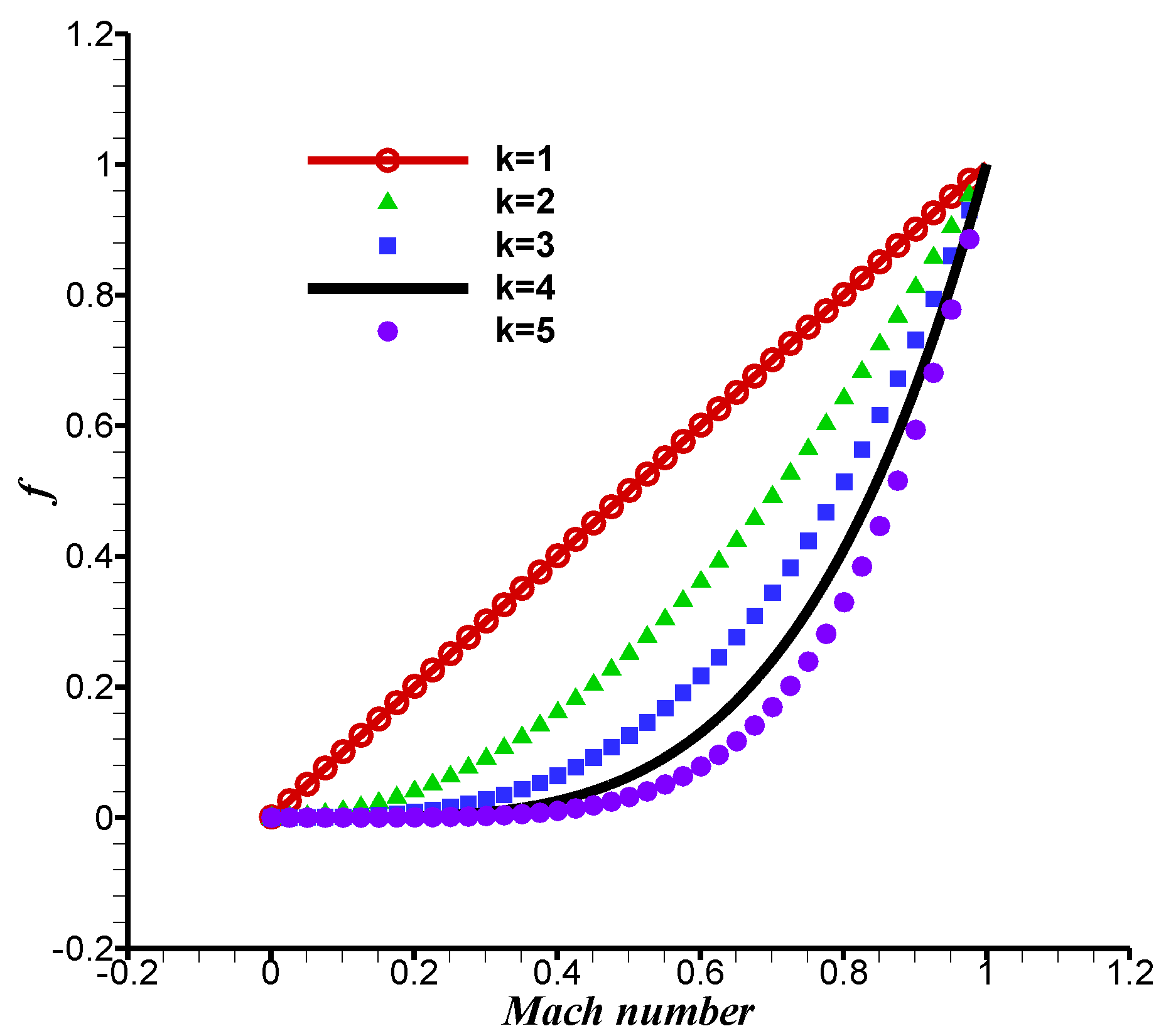
Figure 2 shows that the function f changes with different k’s definitions. However, the disparity becomes smaller with k becoming larger. In fact, our private computations show that the numerical dissipation is nearly unchangeable when $k\ge 3$. Thus, we define the function f and the pressure flux as follows:

$${\widehat{p}}_{i+1/2}=\frac{p_{i+1/2}^{+}+p_{i+1/2}^{-}}{2}+f\cdot d_p$$

(118)

$$f=\min \left({\left|M\right|}^3,1\right)$$

(119)

All in all, with the mass flux defined in Equation (105) and the pressure flux defined in Equation (118), a new low-speed scheme which we call AUSMLS (AUSM for Low speed) is obtained.

5.3. 2D Inviscid NCA0012 Airfoil (Low Speed)

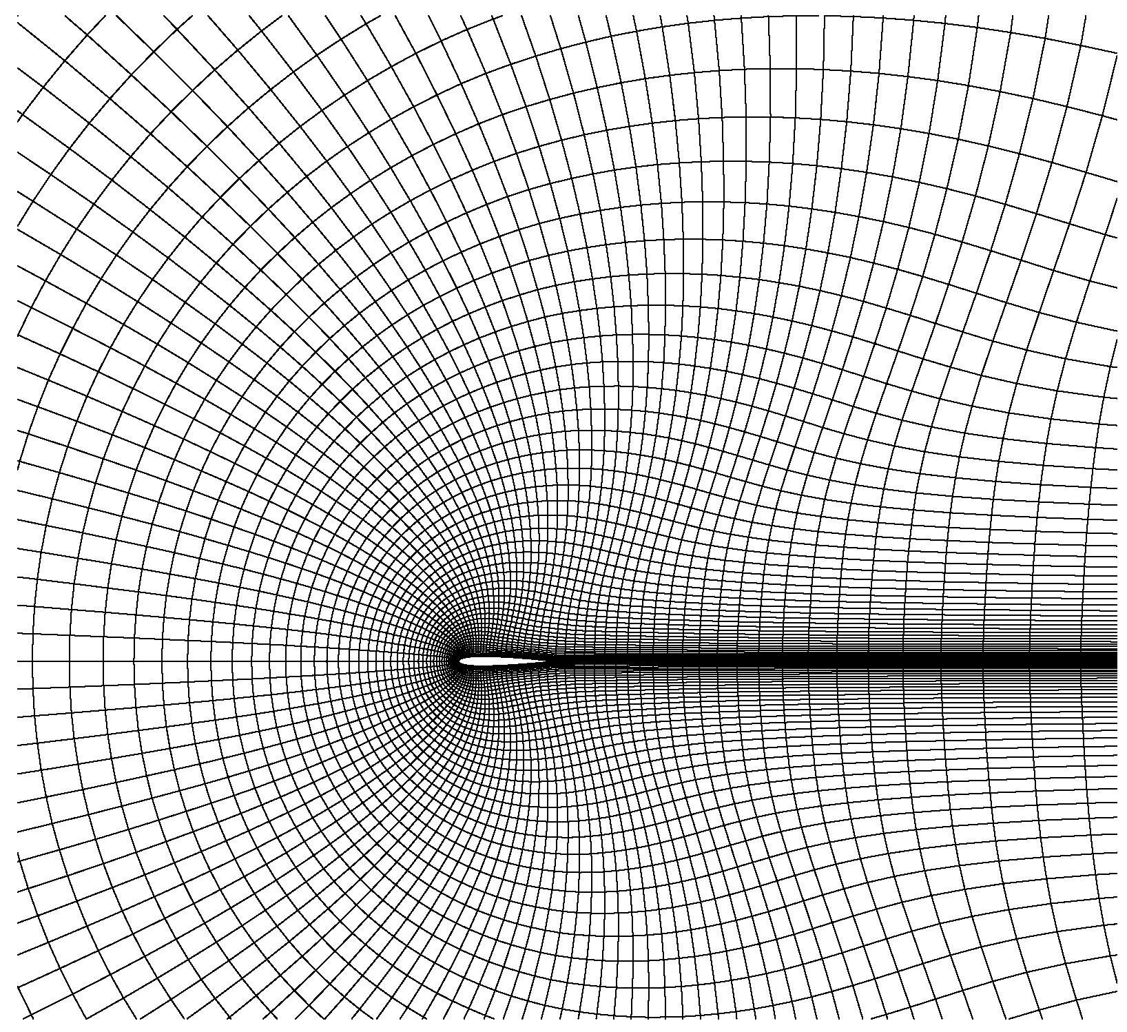
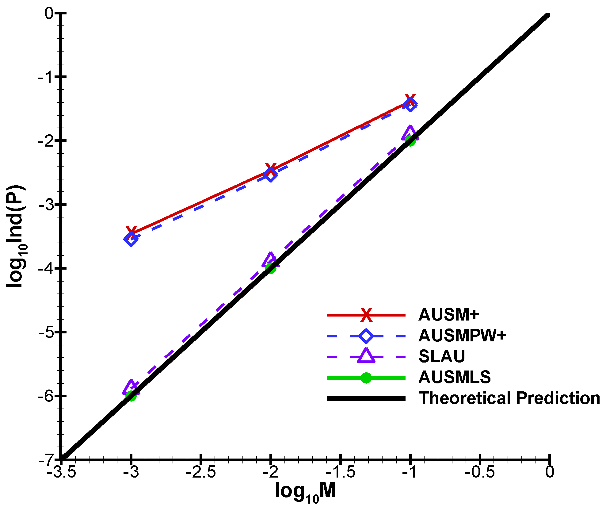
In this section, the accuracy of the AUSMLS scheme in low speed cases is tested. The freestream flow is limited to Ma = 0.001—0.1 with no angle of attack. The grid consists of 120 (circumferential) × 50 (wall normal) (Figure 3). In terms of the spatial accuracy, a fair comparison is conducted between the first order reconstruction method and the AUSM-type schemes. In terms of the time integration, the implicit LU-SGS approach is adopted with the CFL number set to 5, and all the cases are conducted for 100,000 steps to ensure that the density residual reduces six orders at least. Figure 4 depicts the pressure fluctuation with the Mach number obtained by different schemes, in which the Ind(p) is defined as Ind(p) = (P_max − P_min)/P_max. In the continuous cases, the fluctuations of the pressure should scale with the square of the Mach number according to the predictions of theoretical asymptotic. Therefore, AUSMLS is the only one that is able to agree with the theoretical prediction at low speeds while the others, including SLAU, are unable to. Furthermore, it is in accord with the conclusion in Section 4.2 that SLAU performs much better than AUSMPW+ and AUSM+ at low speeds.

6. The AUSMLS Scheme’s Improvements for All Speeds

6.1. Improvement on the Robustness against the Shock Anomaly

In this section, we will conduct a theoretical analysis on the shock anomaly and propose a solution for it.

6.1.1. Quirk’s Test (Odd Even Decoupling)

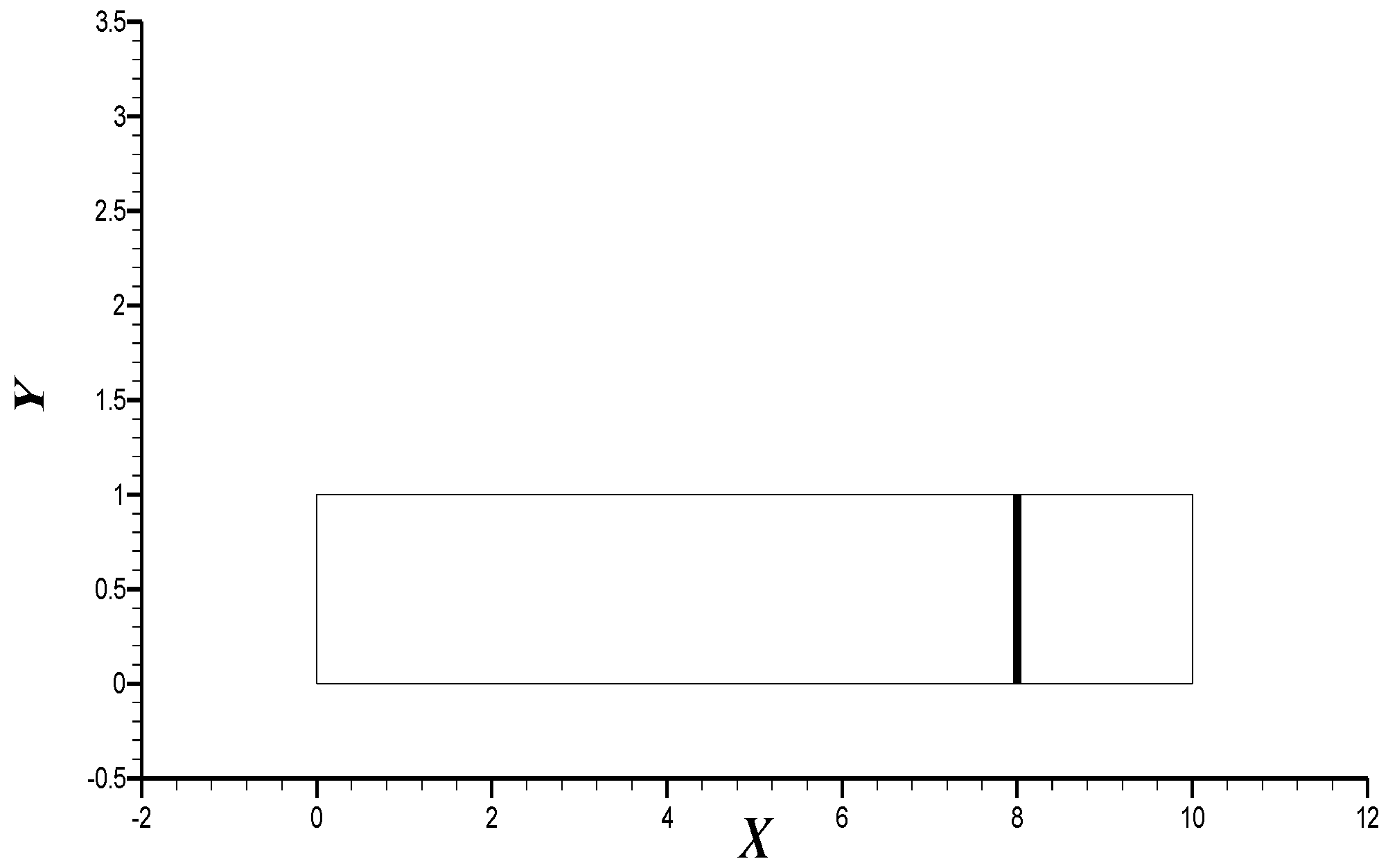
The test called ‘odd–even decoupling’ is proposed by Quirk to examine the robustness against the shock anomaly of the schemes. This test describes a plane moving shock wave in a duct with the centerline grids perturbing. Through analyses, Quirk found that any scheme that does not survive it is not robust against the shock anomaly. The initial conditions of this test produce a normal shock propagate to the left with the Mach number of 6 and are set as ${(\rho ,u,v,p)}_L=(1,6,0,1) , {(\rho ,u,v,p)}_R=(5.25,0.353,0,40.64)$. The shock is located at x = 8 initially with the computational domain [0:1, 0:10] as shown in Figure 5. Moreover, the perturbations of the centerline grids are set as follows:

$$Y_{i,j,mid}=\left\{\begin{array}{ll}{Y}_{j,mid}+{10}^{-4}& for i even\\ Y_{j,mid}-{10}^{-4}& for i odd\end{array}\right.$$

(120)

Following Quirk’s report, we adopt a computational mesh with a nominally uniform grid of 80 (Y) × 200 (X) cells to conduct the analyses. As can be seen in Figure 6, AUSMLS is not robust against the shock anomaly.

6.1.2. Subsubsection

In this section, we would like to examine in detail how the AUSMLS scheme evolves sawtooth-type data by Quirk’s test in Section 6.1.1.

Assuming the solution at time tⁿ is given as follows:

If i is even, then

$${\rho }_i^n=\rho +\Delta {\rho }_i^n, p_i^n=p+\Delta p_i^n, u_i^n=u^0, v_i^n=v^0$$

(121)

else if i is odd, then

$${\rho }_i^n=\rho -\Delta {\rho }_i^n, p_i^n=p-\Delta p_i^n, u_i^n=u^0, v_i^n=v^0$$

(122)

where $\Delta \rho , \Delta p$ are the amplitudes of the density and the pressure perturbations.

The solution at time tⁿ⁺¹ can be expressed as:

$$\Delta p_i^{n+1}=\left(1-2v_y\right)\Delta p_i^n+2v_y\frac{\gamma -1}{{\tilde{c}}^2}\left[\frac{\left({\tilde{u}}^2+{\tilde{v}}^2\right)}{2}\left(1-2\tilde{c}{D}_{Roe}^P-\frac{2D_{Roe}^{\rho }}{\tilde{c}}\right)-{\tilde{v}}^2\right]\Delta p_i^n$$

(123)

$$\Delta {\rho }_i^{n+1}=\left(1+\frac{4v_y{D}_{Roe}^{\rho }}{\tilde{c}}\right)\Delta {\rho }_i^n+\frac{4v_y{D}_{Roe}^P}{\tilde{c}}\Delta p_i^n$$

(124)

where $v_y=\frac{c\Delta t}{\Delta y}$.

Combined with Equations (106)–(109), we can also express the AUSMLS scheme’s amplitudes in Equations (123) and (124) as follows:

$$\Delta p_i^{n+1}=\left(1-2v_y\right)\Delta p_i^n-2v_y\left(\gamma -1\right){\tilde{M}}^2\Delta p_i^n$$

(125)

$$\Delta {\rho }_i^{n+1}=\left(1-2v_y\left|\tilde{M}\right|\right)\Delta {\rho }_i^n-\frac{2v_y}{{\tilde{c}}^2}\left(1-\left|\tilde{M}\right|\right)\Delta p_i^n$$

(126)

As can be seen in Equations (123)–(126), the density field is perturbed by the perturbation of the pressure. The coefficients $D^p$ and $D^{\rho }$ are capable of controlling the perturbations. Thus, three methods can be used to improve the robustness of the scheme against the shock anomaly. They are: (a) control the density contribution by modifying the coefficient $D^{\rho }$, (b) control the pressure contribution by modifying the coefficient $D^p$, (c) control the density and the pressure contributions at the same time by modifying both the coefficient $D^p$ and the coefficient $D^{\rho }$. In fact, Kim adopted the methods (b), (c) and proposed a scheme called RoeM-type which has robustness against the shock anomaly [33]. However, Equation (123) and Equation (125) show that the coefficient $D^p$ would be of the order O(M^k) (k is larger than 1) if we modify the AUSMLS’s mass flux by adopting the methods (b) and (c) as Kim, and this is contradicts the Lemma 1 in Section 4.3.1. Thus, we would like to choose the method (a) to improve the robustness of the scheme against the shock anomaly at high speeds and to avoid the unphysical phenomenon at low speeds. Therefore, we modify the coefficient D^ρ to the following form:

$$D_{i+1/2,j}^{\rho }=-\frac{\tilde{c}}{2}{\left|\tilde{M}\right|}^d$$

(127)

$$d=\frac{\left|\tilde{M}\right|}{II}$$

(128)

where

$$II=\left\{\begin{array}{ll}{\left|\tilde{M}\right|}^{h_{ 1}}& \left|\tilde{M}\right|<1\\ \left|\tilde{M}\right|& {\tilde{u}}^2+{\tilde{v}}^2=0\end{array}\right.$$

(129)

with

$$h_1=\min \left(f_{p1},f_{p2},f_{p3},f_{p4},f_{p5}\right)$$

(130)

$$f_{p1}=P_{i+1/2,j}, f_{p2}=P_{i,j-1/2}, f_{p3}=P_{i,j+1/2}, f_{p4}=P_{i+1,j-1/2}, f_{p5}=P_{i+1,j+1/2}$$

(131)

$$P_{i+1/2,j}=\min \left(\frac{p_{i,j}}{p_{i+1,j}},\frac{p_{i+1,j}}{p_{i,j}}\right)$$

(132)

It is reminded that previous studies show that the coefficient D^ρ should satisfy the following equation to capture the contact discontinuity accurately [29]:

$$D_{i+1/2,j}^{\rho }=-\frac{\left|{\tilde{V}}_n\right|}{2}$$

(133)

Therefore, we define t = 1 if the function P1 is equal to 1.

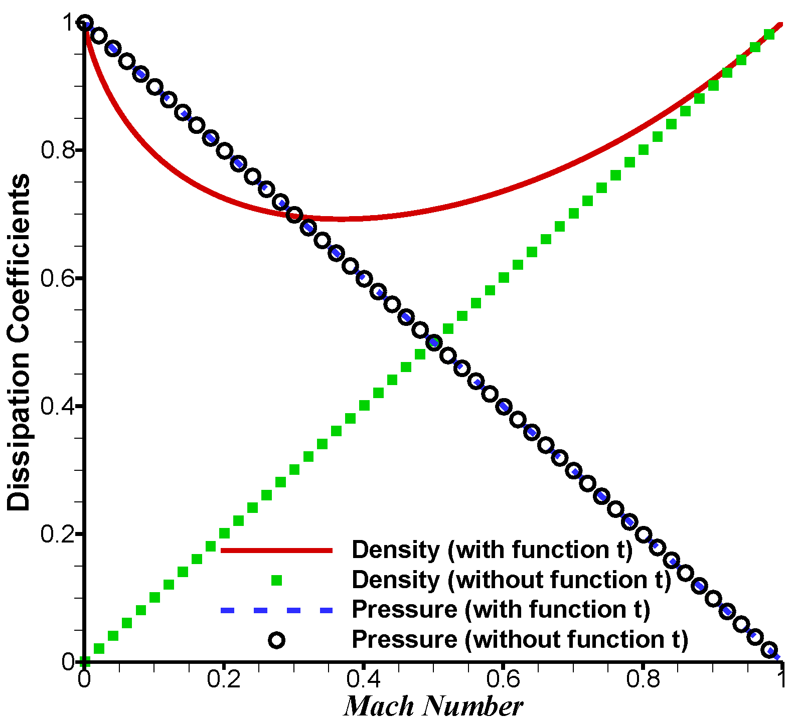
Figure 7 shows the distributions of the dissipative coefficients in the case where h₁ is equal to 0. It should be noticed that the coefficient $D^{\rho }$ is divided by −2 and the coefficient $D^p$ is divided by −2c² for uniformity. As shown in Figure 7, the dissipative coefficients of the density and the pressure are balanced by using the function t. Furthermore, the dissipation coefficient of the density keeps larger than that of no function t.

6.2. Improvement on the Robustness against the Unphysical Expansion Shock

Through theoretical analysis, Einfeldt found that the underestimation of the numerical signal velocities might cause the failure of the scheme in distinguishing expansion shocks from compression ones [34]. To be from the unphysical expansion shock’s appearance, he incorporated the neighboring cells’ values to compute the numerical signal velocity. In this paper, we borrow this idea and the non-linear eigenvalues of Equation (109) can be modified to the following forms:

$$\begin{array}{l}{\left|{\lambda }_1\right|}^{\prime }=\left|{\tilde{V}}_n\right|=\left|{\lambda }_1\right|\\ {\left|{\lambda }_2\right|}^{\prime }=\max \left(\left|{\tilde{V}}_n+\tilde{c}\right|,\left|{\left(V_n\right)}_{i+1/2}^{+}+\tilde{c}\right|\right)\\ {\left|{\lambda }_3\right|}^{\prime }=\min \left(\left|{\tilde{V}}_n-\tilde{c}\right|,\left|{\left(V_n\right)}_{i+1/2}^{-}-\tilde{c}\right|\right)\end{array}$$

(134)

6.3. The All-Speed AUSM-Type Scheme

Based on the analyses above, the newly all-speed AUSM-type scheme which we call AUSMAS is as follows:

$$\begin{array}{ll}{\mathit{f}}_{c,i+1/2}^{\mathrm{AUSMAS}}=& \frac{{\widehat{m}}_{i+1/2}^{\mathrm{AUSMAS}}+\left|{\widehat{m}}_{i+1/2}^{\mathrm{AUSMAS}}\right|}{2}{\mathit{q}}_{i+1/2}^{+}+\hfill \\ & \frac{{\widehat{m}}_{i+1/2}^{\mathrm{AUSMAS}}-\left|{\widehat{m}}_{i+1/2}^{\mathrm{AUSMAS}}\right|}{2}{\mathit{q}}_{i+1/2}^{-}+{\widehat{p}}_{i+1/2}^{\mathrm{AUSMAS}}N\hfill \end{array}$$

(135)

where

$${\widehat{m}}_{i+1/2}^{\mathrm{AUSMAS}}=\frac{1}{2}\left[{\left(\rho V_n\right)}_{i+1/2}^{+}+{\left(\rho V_n\right)}_{i+1/2}^{-}\right]+D_{\mathrm{AUSMAS}}^{\rho }\Delta \rho +D_{\mathrm{AUSMAS}}^{V_n}\Delta V_n+D_{\mathrm{AUSMAS}}^p\Delta p$$

(136)

$$D_{\mathrm{AUSMAS}}^p=\frac{2{\left|{\lambda }_1\right|}^{\prime }-\left({\left|{\lambda }_2\right|}^{\prime }+{\left|{\lambda }_3\right|}^{\prime }\right)}{4{\tilde{c}}^2}$$

(137)

$$D_{\mathrm{AUSMAS}}^{V_n}=\frac{\left({\left|{\lambda }_3\right|}^{\prime }-{\left|{\lambda }_2\right|}^{\prime }\right)}{4\tilde{c}}$$

(138)

$${\widehat{p}}_{i+1/2}^{\mathrm{AUSMAS}}=\frac{p_{i+1/2}^{+}+p_{i+1/2}^{-}}{2}+f\cdot d_p$$

(139)

Moreover, the function t is in the form of Equation (128), the function f is in the form of Equation (119), and the function d_p is in the form of Equation (114).

6.4. Analysis on the AUSMAS Scheme’s Behavior at Low Speeds

As can be seen in Section 5.1, Section 5.2, Section 5.3, Section 6.1, Section 6.2 and Section 6.3, the differences between AUSMAS and AUSMLS lie in the definitions of the coefficient $D^{\rho }$ and the non-linear eigenvalues. In this section, we would like to give a brief proof to show that these differences have little influence on the schemes’ resolutions at low speeds.

Lemma 3.

The difference of the coefficient D^ρ has little influence on the performance of scheme at low speeds.

Proof. 

As stated in Section 4.1, in low Mach limit, the physical pressure is proportional to the square of the Mach number. Thus, the function h₁ in Equation (130) approaches 1 when the Mach number approaches 0. Correspondingly, the function t in Equation (126) approaches 1 and the coefficient D^ρ in Equation (139) is equal to the AUSMLS scheme’s in Equation (106). Thus, the difference of the coefficient D^ρ has little influence on the schemes’ performances at low speeds. □

Lemma 4.

The modifications of the non-linear eigenvalues have little influence on the performance of the scheme at low speeds.

Proof. 

In the low Mach number limit, V_n is quite small and the modification of it can be disregarded at low speeds. Therefore, the performance of the scheme at low speeds is little influenced by the non-linear eigenvalues’ modifications. □

All in all, AUSMAS is almost the same as AUSMLS at low speeds.

7. Numerical Experiments

7.1. Sod Shock Tube

The initial conditions are given as ${(\rho ,u,p)}_L=(1,0,1), {(\rho ,u,p)}_R=(0.125,0,0.1)$ with a computational grid of 400 cells. In terms of the time integration, the explicit fourth Runge–Kutta time-marching scheme is employed and the CFL number is equal to 0.5 in terms of the spatial accuracy; all these flux schemes are conducted with the first order reconstruction method.

Figure 8 depicts density and pressure distributions obtained by different schemes at 1.8 s. As shown in the figure, the AUSMAS is able to produce similar steep gradients near the contact discontinuity and the shock as the others.

7.2. Sod Shock Tube II

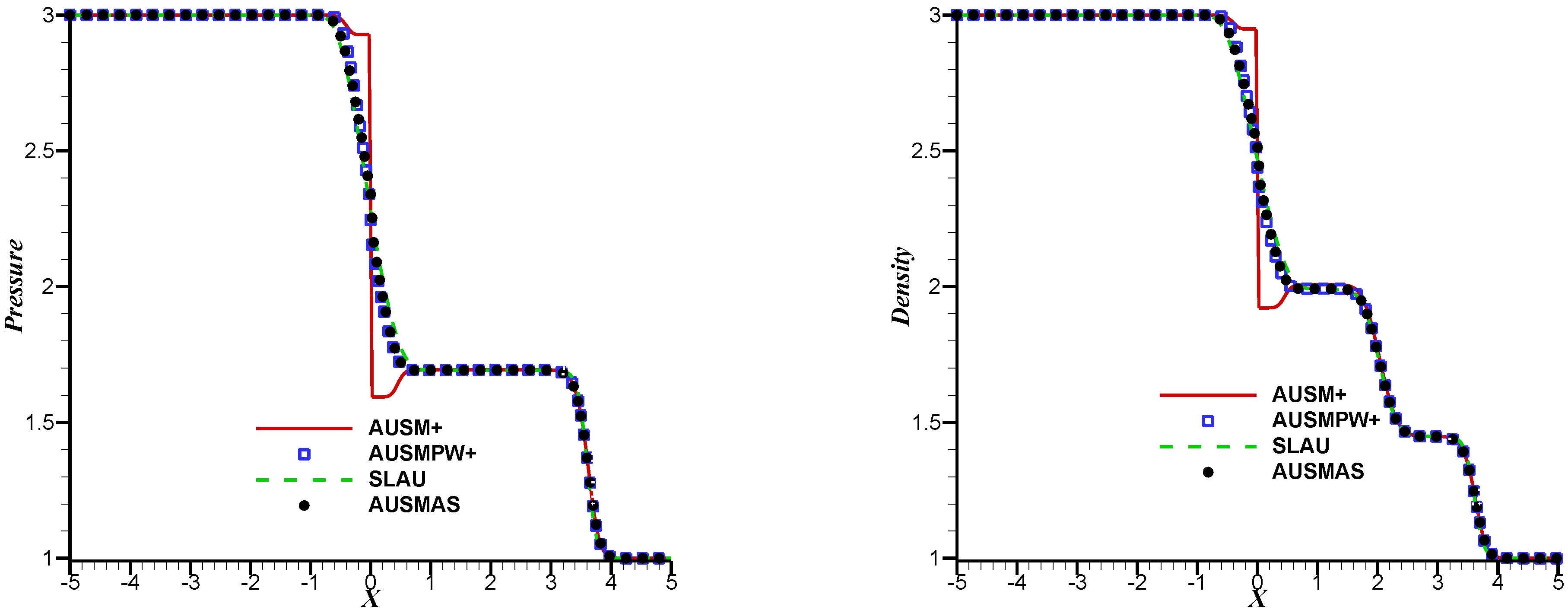
In this test, the initial conditions are given as ${(\rho ,u,p)}_L=(3,0.9,3), {(\rho ,u,p)}_R=(1,0.9,1)$. The length of the domain is 10 and is discretized with 400 cells. The explicit fourth Runge–Kutta time-marching scheme is adopted with the CFL number set to 0.5. In terms of the spatial accuracy, the first order reconstruction method is employed.

The schemes’ pressure distributions and density distributions at 1.5 s are depicted in Figure 9. As can be seen in them, AUSM+ yields an unphysical expansion shock. AUSMAS is capable of avoiding this unphysical phenomenon like AUSMPW+ and SLAU. Therefore, AUSMAS is robust against the unphysical expansion shock.

7.3. 2D Inviscid NCA0012 Airfoil

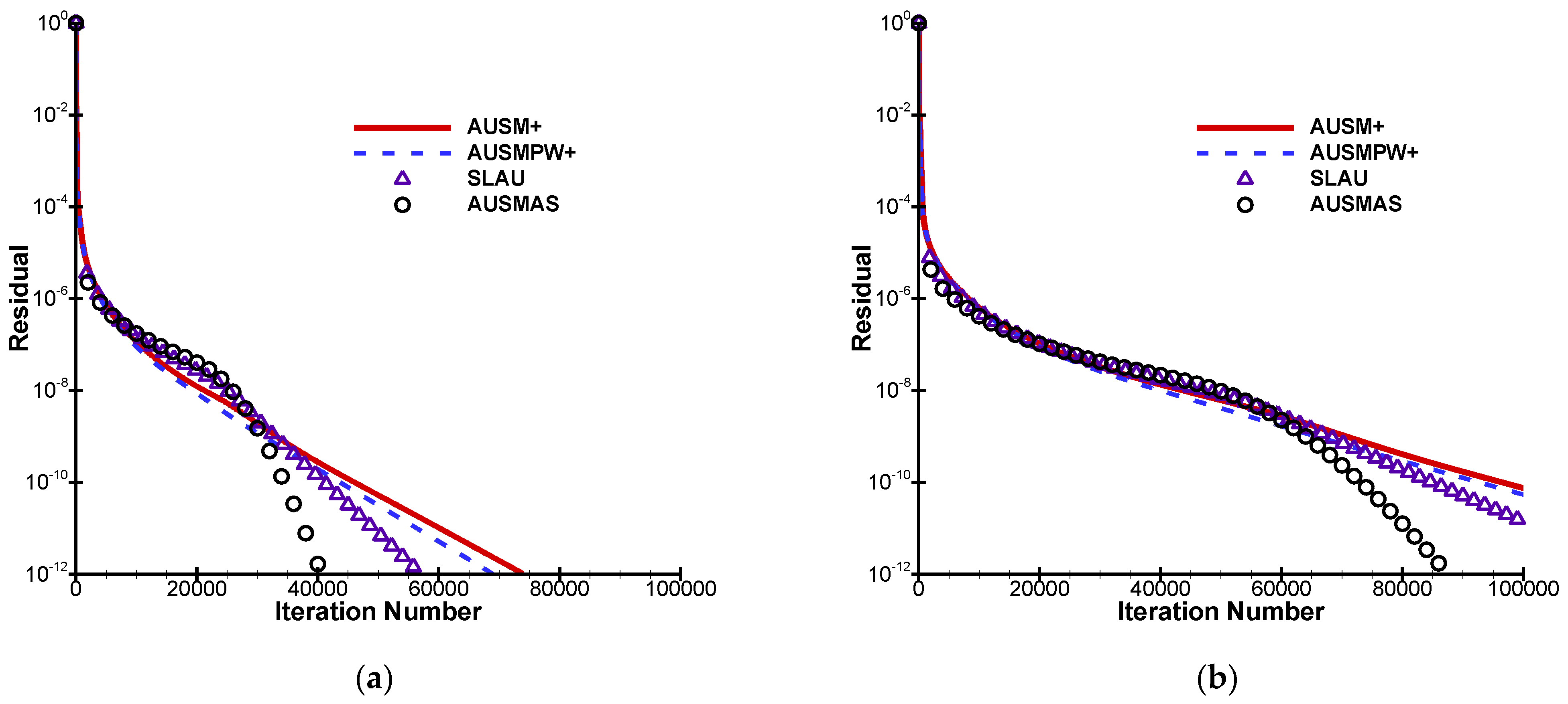
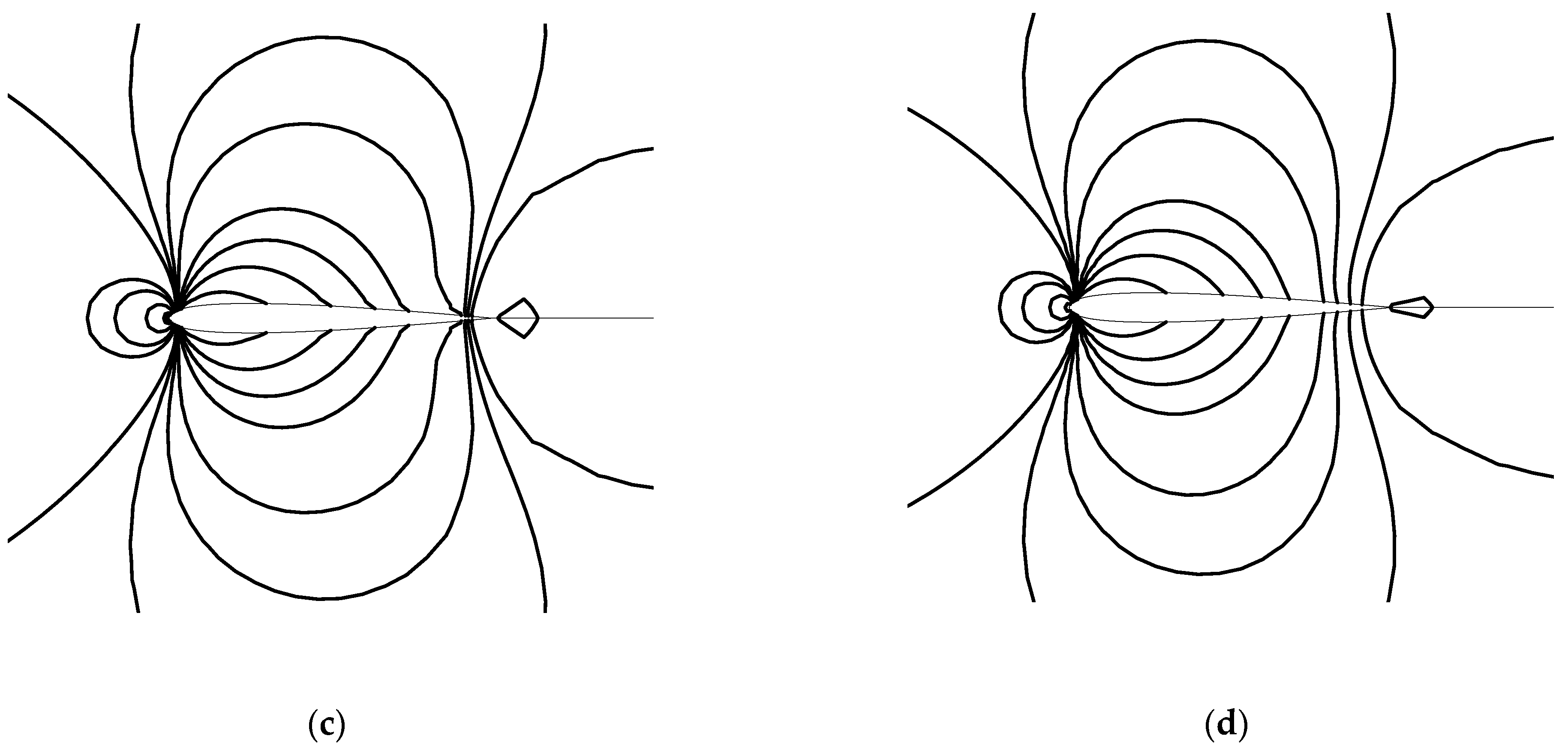
The flow conditions and the calculating settings are the same as those in Section 5.3. Furthermore, the computations within the two different grids are conducted to check the grid dependencies of the schemes, in which the grid with 120 (circumferential) × 50 (wall normal) is called the coarse grid (Figure 3) and another with 240 (circumferential) × 100 (wall normal) is called the dense grid. In addition, we adopt three different reconstruction methods to analyze the schemes’ disparities. These reconstruction technologies including the reconstruction of first order, MUSCL reconstruction of second order combined with van Leer limiter [28], third order reconstruction combined with van Leer limiter [35]. In terms of the time integration, the CFL number is equal to 10 with the implicit LU-SGS approach adopted. To achieve at least ten orders reduction of the density residual, all the computations are conducted for 100,000 steps. The error histories of these schemes combined with first reconstruction method in different grids are shown in Figure 10. In them we can see that all the computations are convergent after iterating 100,000 steps and AUSMAS converges much faster than the others. Figure 11 indicates that AUSMAS and SLAU are capable of obtaining accurate flow fields at low speeds while the others obtain inaccurate ones. Furthermore, the AUSMAS scheme avoids the weak oscillations in the vicinity of the wall while SLAU scheme is inclined to show this unphysical phenomenon.

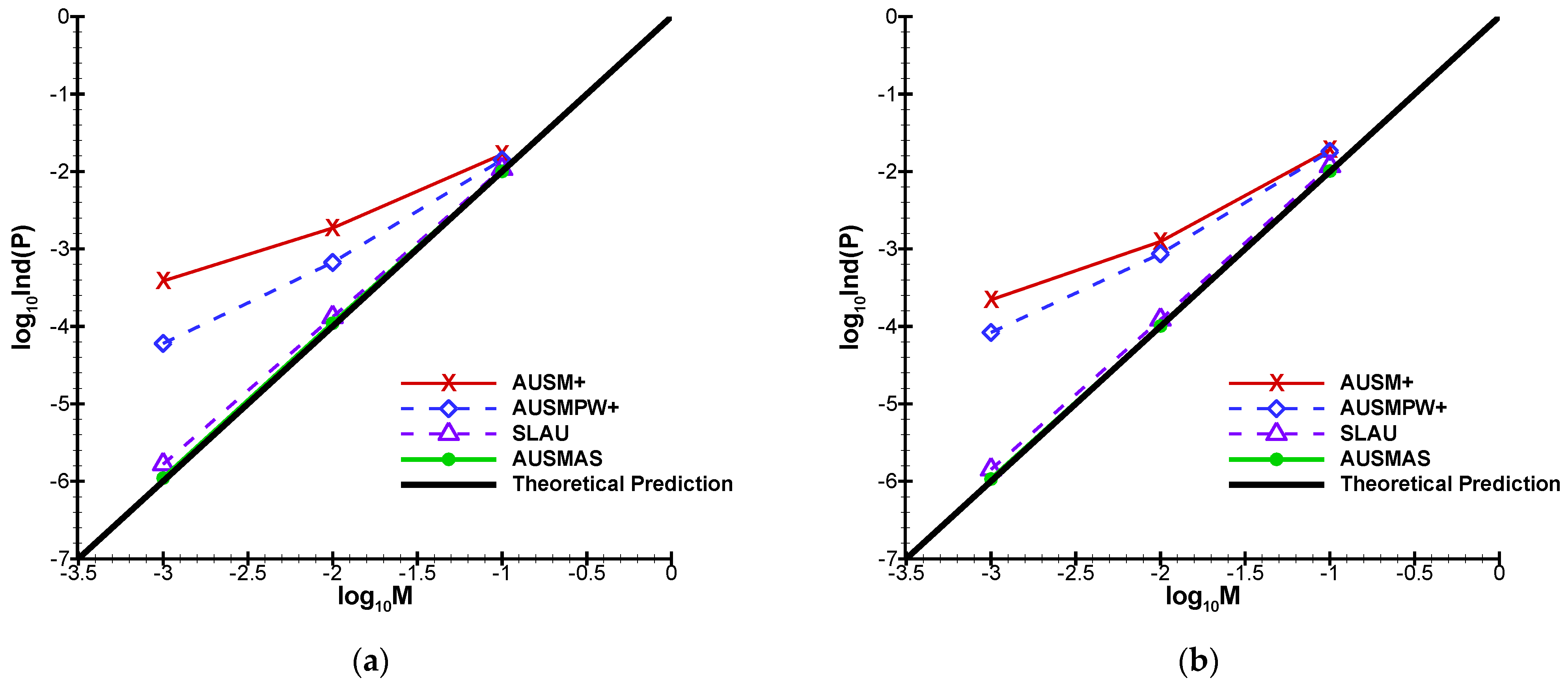
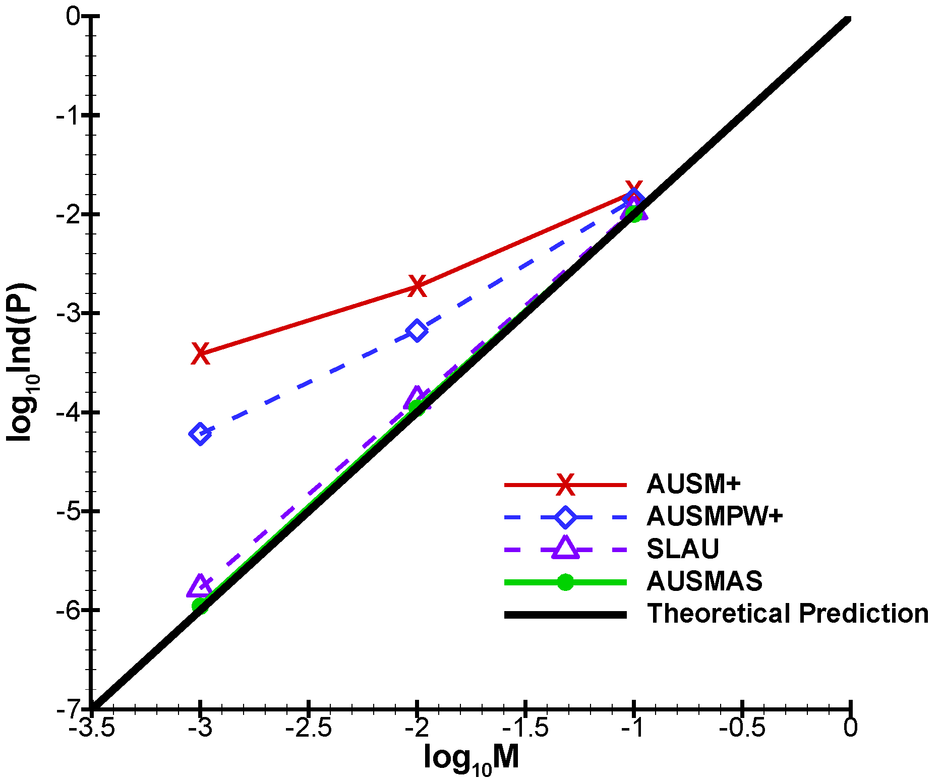
Figure 12a depicts the pressure fluctuations of the schemes vs. the Mach number with first order reconstruction method. In this paper, the pressure fluctuation is defined as Ind(p) = (P_max − P_min)/P_max.

According to the theoretical asymptotic prediction, in the continuous case, the pressure fluctuation is proportional to the square of the Mach number. Therefore, none of these schemes are able to agree with the theoretical predictions except for the AUSMAS scheme.

Figure 12b,c display the pressure fluctuations obtained by different schemes coupled with reconstruction methods of higher order. In them, we can find that only AUSMAS is able to obtain the physical solutions no matter which reconstruction method it is combined with at low speeds. Furthermore, the result of the AUSMAS scheme with the reconstruction method of first order is even better than the results of the other schemes combined with higher order reconstruction methods.

Similarly, Figure 13 indicates that AUSMAS performs the best among all these schemes in the dense grid.

In theory, the drag coefficient of the airfoil should be 0 in this case. Therefore, the drag coefficient is also a good measurement of the schemes’ numerical errors [36].

Figure 14 and Figure 15 display the drag coefficients obtained by different schemes with different reconstruction methods or different computational grids. As can be seen in the results, the numerical error of the AUSMAS is much less than others in all these cases.

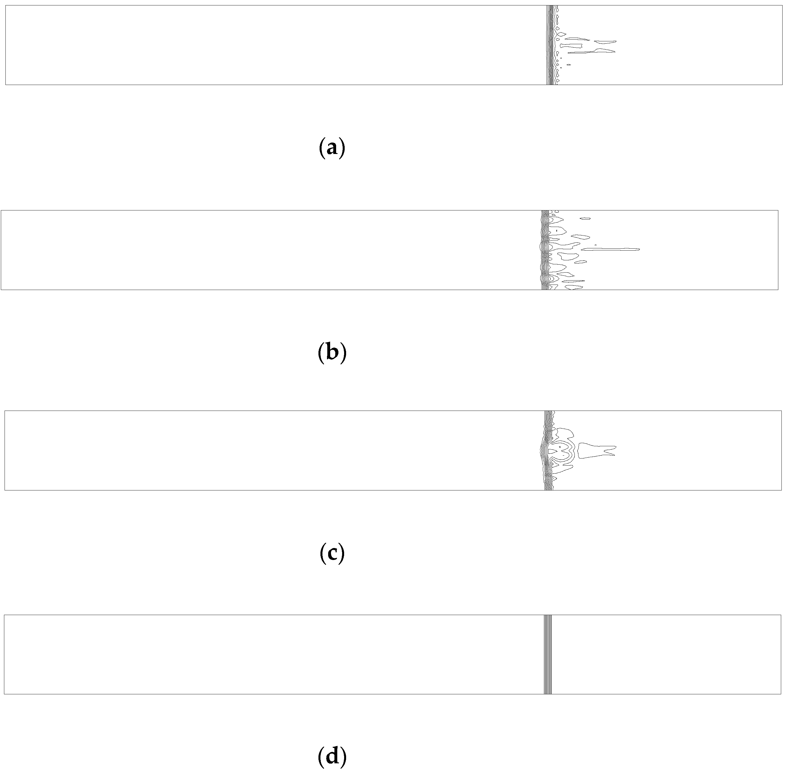
7.4. Quirk’s Test (Odd–Even Decoupling)

In this section, all the initial conditions including the initial location of the shock and the computational domain are the same as those in Section 6.1.1. Moreover, the perturbations of the centerline grids are given in Equation (120) [37,38,39]. In terms of the time integration, the methodology of explicit fourth Runge–Kutta time-marching is applied.

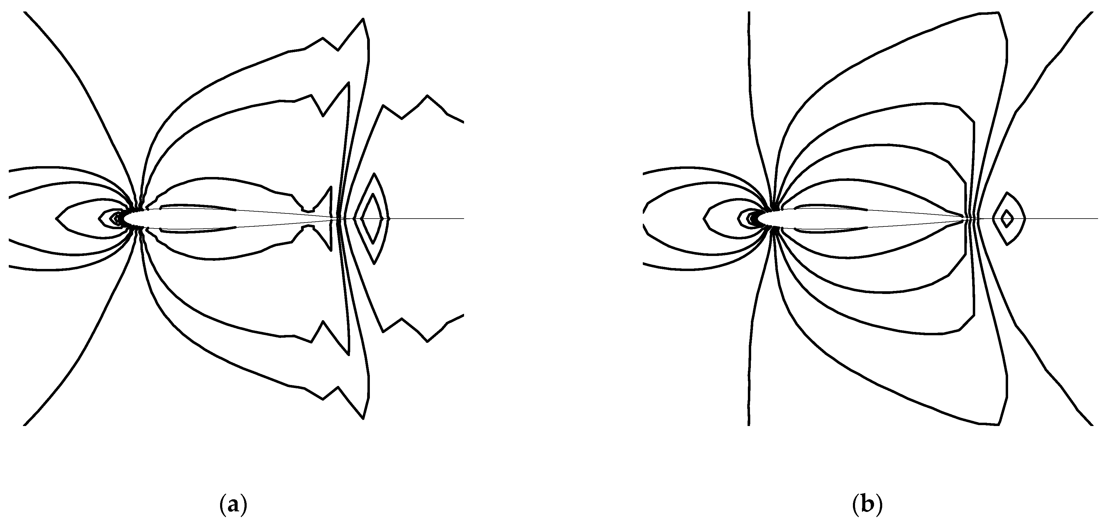
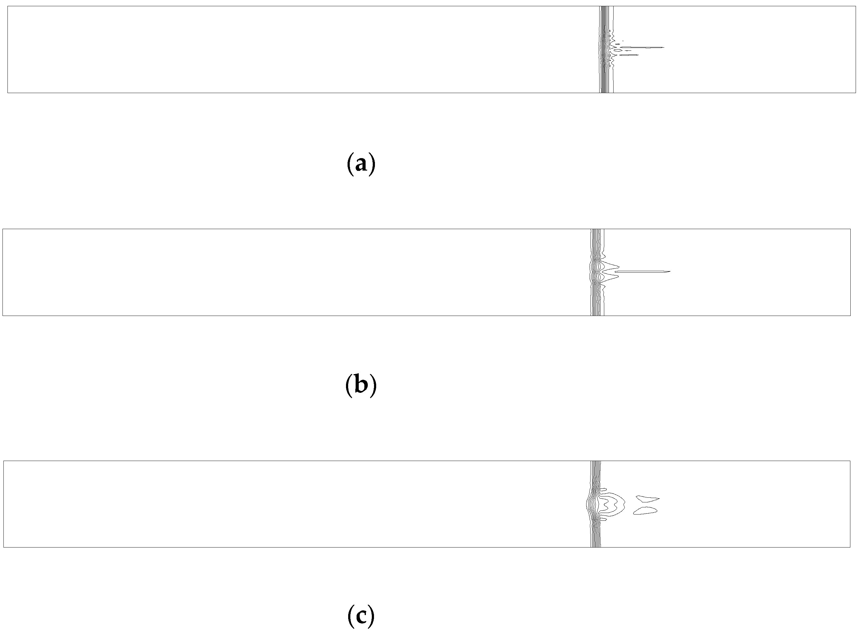
As can be seen in Figure 16, AUSMAS is the only one which is able to be robust against the abnormal shock. Figure 17 shows the density contours of all these schemes combined with the MUSCL reconstruction method of second order. In it we can see that AUSMAS is still the only one to be free from the appearance of the unphysical shock anomaly.

8. Conclusions Remarks

In this paper, a new AUSM-type scheme called AUSMAS is proposed. Theoretical analyses are conducted in Section 4, Section 5 and Section 6 and they indicated that the AUSMAS scheme has the following two advantages, independent of any tuning coefficient: (a) for low speeds, it gains a high level of accuracy when the Mach number approaches to 0, (b) for high speeds, it is robust against the shock anomaly and free from the appearance of the unphysical expansion shocks. Two one-dimensional test cases (Section 7.1 and Section 7.2) show that AUSMAS is able to capture the shocks and contact discontinuities as sharply as other schemes including SLAU, AUSM+ and AUSMPW+. Moreover, it is free from the appearance of the unphysical expansion shocks in supersonic/hypersonic flow simulations. In Section 7.3, AUSMAS displays its high resolution at low speeds. Quirk’s test in Section 7.4 shows that AUSMAS is robust against the shock anomaly while the others are not. Furthermore, other methods can not satisfy these merits at the same time.

All in all, AUSMAS can be widely used in both engineering applications and in research due to its high resolution, efficiency and robustness at all speeds.

References

- Liou, M.S.; Steen, C.J., Jr. A new flux splitting scheme. J. Comp. Phys. 1993, 107, 23–39. [Google Scholar] [CrossRef] [Green Version]
- Liu, Y.; Shi, Y.; Tong, M.; Zhao, F.; Chen, B. Aeroacoustic Investigation of Passive and Active Control on Cavity Flowfields Using Delayed Detached Eddy Simulation. Int. J. Aerosp. Eng. 2019, 2019, 2650842. [Google Scholar] [CrossRef]
- Qu, F.; Sun, D.; Bai, J.Q.; Zuo, G.; Yan, C. Numerical investigation of blunt body’s heating load reduction with combination of spike and opposing jet. Int. J. Heat Mass Transf. 2018, 127, 7–15. [Google Scholar] [CrossRef]
- Liou, M.S.; Steen, C.J., Jr. A sequal to AUSM: AUSM+. J. Comp. Phys. 1996, 129, 364–382. [Google Scholar] [CrossRef]
- Kim, K.H.; Lee, J.; Rho, O.H. An improvement of AUSM schemes by introducing the pressure-based weight functions. Comput. Fluids 1998, 27, 311–346. [Google Scholar]
- Kim, K.H.; Kim, C.; Rho, O.H. Methods for the Accurate Computations of Hypersonic Flows I. AUSMPW+ Scheme. J. Comp. Phys. 2001, 174, 38–80. [Google Scholar] [CrossRef]
- Liou, M.S. A Further Development of the AUSM_ Scheme Towards Robust and Accurate Solutions for All Speeds. In Proceedings of the AIAA Computational Fluid Dynamics Conference, Orlando, FL, USA, 23–26 June 2003. AIAA Paper 2003-4116. [Google Scholar]
- Kitamura, K.; Shima, E. Parameter-Free Simple Low-Dissipation AUSM-Family Scheme for All Speeds. AIAA J. 2011, 49, 1693–1709. [Google Scholar]
- Qu, F.; Yan, C.; Yu, J.; Sun, D. A study of parameter-free shock capturing upwind schemes on low speeds’ issues. Sci. China Tech. Sci. 2014, 57, 1183–1190. [Google Scholar] [CrossRef]
- Weiss, J.M.; Smith, W.A. Preconditioning applied to variable and constant density flows. AIAA J. 1995, 33, 2050–2057. [Google Scholar] [CrossRef]
- Turkel, E. Preconditioning technique in Computational Fluid Dynamics. Annu. Rev. Fluid Mech. 1999, 31, 385–416. [Google Scholar] [CrossRef]
- Unrau, D.; Zingg, D.W. Viscous airfoil computations using local preconditioning. In Proceedings of the 13th Computational Fluid Dynamics Conference, Snowmass Village, CO, USA, 29 June–2 July 1997. AIAA Paper 1997-2027. [Google Scholar]
- Li, X.S.; Xu, J.Z.; Gu, C.W. Preconditioning method and Engineering application of Large Eddy simulation. Sci. China Ser. G Phys. Mech. Astron. 2008, 51, 667–677. [Google Scholar] [CrossRef]
- Li, X.S.; Gu, C.W.; Xu, J.Z. Development of Roe-type scheme for all-speed flows based on preconditioning method. Comput. Fluids 2009, 38, 810–817. [Google Scholar] [CrossRef]
- Durante, D.; Rossi, E.; Colagrossi, A.; Graziani, G. Numerical simulations of the transition from laminar to chaotic behaviour of the planar vortex flow past a circular cylinder. Commun. Nonlinear Sci. Numer. Simul. 2017, 48, 18–38. [Google Scholar] [CrossRef]
- Qu, F.; Chen, J.; Sun, D.; Bai, J.; Yan, C. A new all-speed flux scheme for the Euler equations. Comput. Math. Appl. 2019, 77, 1216–1231. [Google Scholar] [CrossRef]
- Dellacherie, S.; Jung, J.; Omnes, P.; Raviart, P.-A. Construction of modified Godunov—Type schemes accurate at any Mach number for the compressible Euler system. Math. Models Methods Appl. Sci. 2016, 26, 2525–2615. [Google Scholar] [CrossRef] [Green Version]
- Li, X.S.; Gu, C.W. Mechanism of Roe-type schemes for all-speed flows and its application. Comput. Fluids 2013, 86, 56–70. [Google Scholar] [CrossRef] [Green Version]
- Kitamura, K.; Shima, E. Carbuncle Phenomena and Other Shock Anomalies in Three Dimensions. AIAA J. 2012, 50, 2655–2669. [Google Scholar] [CrossRef] [Green Version]
- Xie, W.; Li, W.; Li, H.; Tian, Z.; Pan, S. On numerical instabilities for Godunov-type schemes for strong shocks. J. Comput. Phys. 2017, 350, 607–637. [Google Scholar] [CrossRef]
- Qu, F.; Sun, D.; Zhou, B.; Bai, J. Self-similar structures based genuinely two-dimensional Riemann solvers in curvilinear coordinates. J. Comput. Phys. 2020, 420, 109668. [Google Scholar] [CrossRef]
- Qu, F.; Sun, D.; Yan, C. A new flux splitting scheme for the Euler equations II: E-AUSMPWAS for All Speeds. Commun. Nonlinear Sci. Numer. Simul. 2018, 57, 58–79. [Google Scholar] [CrossRef]
- Qu, F.; Yan, C.; Sun, D. A new Roe-type scheme for all speeds. Comput. Fluids 2015, 121, 11–25. [Google Scholar] [CrossRef]
- Qu, F.; Sun, D.; Bai, J.Q.; Yan, C. A genuinely two-dimensional Riemann solver for compressible flows in curvilinear coordinates. J. Comput. Phys. 2019, 386, 47–63. [Google Scholar] [CrossRef]
- Qu, F.; Chen, J.; Sun, D.; Bai, J.; Zuo, G. A grid strategy for predicting the space plane’s hypersonic aerodynamics heating loads. Aerosp. Sci. Technol. 2019, 86, 659–670. [Google Scholar] [CrossRef]
- Blazek, J. Computational Fluid Dynamics: Principles and Applications, 1st ed.; Elsevier: Oxford, UK, 2001. [Google Scholar]
- Van Leer, B. Towards the Ultimate Conservation Difference Scheme V: A Second-Order Sequal to Godunov’s Method. J. Comp. Phys. 1979, 32, 101–136. [Google Scholar] [CrossRef]
- Liou, M.S. Mass Flux Schemes and Connection to Shock Instability. J. Comp. Phys. 2000, 160, 623–648. [Google Scholar] [CrossRef]
- Guillard, H.; Viozat, C. On the behaviour of upwind schemes in the low mach number limit. Comput. Fluids 1999, 28, 63–86. [Google Scholar] [CrossRef]
- Guillard, H.; Murrone, A. On the behaviour of upwind schemes in the low mach number limit: II. Godunov type schemes. Comput. Fluids 2004, 33, 655–675. [Google Scholar] [CrossRef] [Green Version]
- Toro, E.F. Riemann Solvers and Numerical Methods for Fluid Dynamics, 3rd ed.; Springer: Berlin/Heidelberg, Germany, 2009. [Google Scholar]
- Roe, P.L. Approximate Riemann solvers, parameter vectors and difference schemes. J. Comp. Phys. 1981, 43, 357–372. [Google Scholar] [CrossRef]
- Kim, S.S.; Kim, C.; Rho, O.H.; Hong, S.K. Cures for the Shock Instability, Development of a Shock-Stable Roe Scheme. J. Comp. Phys. 2003, 185, 342–374. [Google Scholar] [CrossRef]
- Einfeldt, B.; Munz, C.D.; Roe, P.L.; Sjögreen, B. On Godunov-Type methods near low densities. J. Comp. Phys. 1991, 92, 273. [Google Scholar] [CrossRef]
- Kim, K.H.; Kim, C. Accurate, efficient and monotonic numerical methods for multidimensional compressible flows Part II: Multi-dimensional limiting process. J. Comp. Phys. 2005, 208, 570–615. [Google Scholar] [CrossRef]
- Kitamura, K.; Shima, E. Towards shock-stable and accurate hypersonic heating computations: A new pressure flux for AUSM-family schemes. J. Comp. Phys. 2013, 245, 62–83. [Google Scholar] [CrossRef]
- Henderson, J.; Menart, J.A. Grid study on blunt bodies with the Carbuncle Phenomenon. In Proceedings of the 39th AIAA Thermophysics Conference, Miami, FL, USA, 25–28 June 2007. AIAA Paper 97-3904. [Google Scholar]
- Pandolfi, M.; D’Ambrosio, D. Numerical Instabilities in Upwind Methods: Analysis and Cures for the “Carbuncle” Phenomenon. J. Comp. Phys. 2011, 166, 271–301. [Google Scholar] [CrossRef] [Green Version]
- Kim, K.H.; Kim, C.; Rho, O.H. Methods for the Accurate Computations of Hypersonic Flows II. Shock-Aligned Grid Technique. J. Comp. Phys. 2001, 174, 81–119. [Google Scholar] [CrossRef]
Figure 1.
The Cartesian grid.
Figure 2.
Distributions of the function f with different k’s definitions when .
Figure 3.
The computational grid of NACA0012 (120 × 50).
Figure 4.
Pressure fluctuations vs. freestream Mach number (first order reconstruction with computational grid of 120 × 50).
Figure 5.
The initial density contour and axis lines.
Figure 6.
Density contours of the odd–even grid perturbation problem (Ms = 6.0).
Figure 7.
Dissipation coefficients of the pressure and the density.
Figure 8.
Pressure and density distributions of the Sod shock tube test (t = 1.8 s).
Figure 9.
Pressure and density distributions of the Sod shock tube II test (t = 1.5 s).
Figure 10.
Error histories of inviscid flow over NACA0012 airfoil (M∞ = 0.1, first order reconstruction, (a) coarse grid, (b) dense grid).
Figure 11.
Schemes’ pressure contours of inviscid flows around NACA0012 airfoil with the first order reconstruction (Ma = 0.1, coarse grid); (a) AUSM+; (b) AUSMPW+; (c) SLAU; (d) AUSMAS.
Figure 12.
Pressure fluctuations vs inflow Mach number (coarse grid, (a) first order reconstruction, (b) second order reconstruction, (c) third order reconstruction).
Figure 13.
Resolutions of the pressure fluctuations with different schemes (first order reconstruction, dense grid).
Figure 14.
Drag coefficients vs. inflow Mach number (coarse grid, (a) first order reconstruction, (b) second order reconstruction, (c) third order reconstruction).
Figure 15.
Drag coefficients vs. inflow Mach number (first order reconstruction, dense grid).
Figure 16.
Density contours of the odd–even grid perturbation problem (Ms = 6.0, first order reconstruction, ); (a) AUSM+; (b) AUSMPW+; (c) SLAU; (d) AUSMAS.
Figure 17.
Density contours of the odd–even grid perturbation problem (Ms = 6.0, second order MUSCL reconstruction with the minmod limiter, ); (a) AUSM+; (b) AUSMPW+; (c) SLAU; (d) AUSMAS.
Publisher’s Note: MDPI stays neutral with regard to jurisdictional claims in published maps and institutional affiliations. |
© 2022 by the authors. Licensee MDPI, Basel, Switzerland. This article is an open access article distributed under the terms and conditions of the Creative Commons Attribution (CC BY) license (https://creativecommons.org/licenses/by/4.0/).
Share and Cite
MDPI and ACS Style
Li, N.; Qu, F.; Sun, D.; Wu, G. An Effective AUSM-Type Scheme for Both Cases of Low Mach Number and High Mach Number. Appl. Sci. 2022, 12, 5464. https://0-doi-org.brum.beds.ac.uk/10.3390/app12115464
AMA Style
Li N, Qu F, Sun D, Wu G. An Effective AUSM-Type Scheme for Both Cases of Low Mach Number and High Mach Number. Applied Sciences. 2022; 12(11):5464. https://0-doi-org.brum.beds.ac.uk/10.3390/app12115464
Chicago/Turabian StyleLi, Nan, Feng Qu, Di Sun, and Guanghui Wu. 2022. "An Effective AUSM-Type Scheme for Both Cases of Low Mach Number and High Mach Number" Applied Sciences 12, no. 11: 5464. https://0-doi-org.brum.beds.ac.uk/10.3390/app12115464
Note that from the first issue of 2016, this journal uses article numbers instead of page numbers. See further details here.