Rolling Bearing Health Indicator Extraction and RUL Prediction Based on Multi-Scale Convolutional Autoencoder

Abstract

Rolling bearings are some of the most crucial components in rotating machinery systems. Rolling bearing failure may cause substantial economic losses and even endanger operator lives. Therefore, the accurate remaining useful life (RUL) prediction of rolling bearings is of tremendous research importance. Health indicator (HI) construction is the critical step in the data-driven RUL prediction approach. However, existing HI construction methods often require extraction of time-frequency domain features using prior knowledge while artificially determining the failure threshold and do not make full use of sensor information. To address the above issues, this paper proposes an end-to-end HI construction method called a multi-scale convolutional autoencoder (MSCAE) and uses LSTM neural networks for RUL prediction. MSCAE consists of three convolutional autoencoders with different convolutional kernel sizes in parallel, which can fully exploit the global and local information of the vibration signals. First, the raw vibration data and labels are input into MSCAE, and then, MSCAE is trained by minimizing the composite loss function. After that, the vibration data of the test bearings are fed into the trained MSCAE to extract HI. Finally, RUL prediction is performed using the LSTM neural network. The superiority of the HI extracted by MSCAE was verified using the PHM2012 challenge dataset. Compared to state-of-the-art HI construction methods, RUL prediction using MSCAE-extracted HI has the highest prediction accuracy.

1. Introduction

Rolling bearings are the joints of rotating machinery and play an essential role in industrial production, intelligent manufacturing, and transportation [1,2]. Bearing mounting methods, lubricant quality, bearing operating environment, load and speed can all affect bearing vibration and life [3,4,5]. Once the rolling bearing fails, it will cause the machinery and equipment to stop working, causing substantial economic loss or even threatening the operator’s life [6]. Therefore, timely analysis of their working conditions and prediction of their remaining useful life (RUL) is of great research importance [7]. The Prognostic and Health Management (PHM) refers to the use of sensor monitoring data to predict, monitor, and manage the health status of a system through models and algorithms [8,9,10,11,12]. RUL prediction is a crucial technique in PHM and is defined as the time interval between the current moment and when a system or internal component fails [10,11].

Currently, RUL prediction methods are mainly divided into model-based and data-driven methods [13]. The model-based method uses a mathematical approach to construct a physical model of the degradation trend of mechanical components [14]. However, modern mechanical systems have dramatically increased in complexity, have highly coupled internal components, and often operate in severe environments with heavy loads, variable operating conditions, and multiple noise levels [15]. Therefore, building accurate degradation models is a challenging task, limiting the development of model-based methods. The data-driven method is based on machine learning algorithms to construct a mapping relationship between the monitoring data from the sensors and the RUL [16]. Deep learning is currently one of the up-to-date research directions in machine learning. With its powerful data processing and feature extraction capabilities, deep learning is widely used in computer vision, natural language processing, and fault diagnosis [17]. With the advantages of deep learning, more and more researchers are applying it in the RUL prediction model. Wang et al. [18] proposed a multi-scale convolutional attention network. The multi-sensor data are first fused, and then, feature extraction is performed using a multi-scale convolution module with a self-attentive mechanism. Finally, regression analysis is performed on the high-level representation using a dynamic dense layer. The validity of the model was verified using milling tool life data. Ma et al. [19] proposed a convolutional long and short-term memory model for bearing RUL prediction. Unlike the traditional method that directly connects the convolutional neural network (CNN) and LSTM, this method performs convolutional operations on all the state transitions in the LSTM. Cao et al. [20] proposed a temporal convolution prediction framework with a residual self-attention mechanism. The marginal spectrum of the vibration signal is first extracted; then, it is used as the input of the temporal convolution network, and finally, the residual self-attention mechanism is introduced to achieve end-to-end remaining lifetime prediction. The validity of the proposed method was verified with the PHM2012 challenge dataset and the XJTU-SY dataset. Yao et al. [21] proposed a prediction method that combines a one-dimensional convolutional neural network with simple recurrent units.

The extraction of health indicators (HI) is a crucial step in the RUL prediction process. HI mainly reflect the degradation of mechanical equipment. Therefore, the quality of HI will directly affect the RUL prediction accuracy. Qiu et al. [22] used self-organizing mapping (SOM) to fuse the extracted features to construct the HI of rolling bearings. Qin et al. [23] used the root mean square (RMS) error as the HI of a rolling bearing and predicted the future HI sequence using a gated dual attention unit neural network to determine the magnitude of the rolling bearing RUL. Chen et al. [24] proposed a simple HI construction scheme that uses the ratio of the current moment’s RUL value to the initial RUL as the HI, reducing the need for expensive prior knowledge. Five bandpass energy values of the spectrum are used as features. The mapping relationship between the features and HI is constructed directly using a circular autoencoder (AE) based on the attention mechanism. Finally, the value of the RUL is calculated using linear regression. Guo et al. [25] used CNN to extract the bearings’ HI and used outlier region correction techniques to detect and correct the outlier points in the obtained HI.

There are three main problems with the above methods. (1) In the HI construction process, it is often necessary to analyze the vibration signals in the time-frequency domain and extract the features in the time domain, frequency domain or time-frequency domain as the input to the model. However, different combinations of features may produce different results. In the literature [26,27], 14 specially designed features and 14 commonly used features were used for HI construction, respectively, and the trend, monotonicity, and scale similarity of the two HI differed. This approach requires a large amount of expert prior knowledge and does not allow automatic HI extraction. (2) The temporal information of the vibration signals is not fully utilized, and usually, only a single size time window is used for feature extraction of the vibration signals, which cannot utilize the local and the global information comprehensively. The bearing vibration signal is a vector containing time information, and the lack of adequate consideration of the time scale can affect the effectiveness of HI. (3) Usually, when using HI for RUL prediction, the failure threshold of HI needs to be determined. In the literature [23], the RMS maximum value of 1.903 at bearing failure was chosen as the failure threshold. In the literature [28], the failure threshold for HI was determined to be 0.17 by calculating the average of the last five local minimum HI points of the tested motor. These methods often carry a particular element of subjectivity and conjecture, leading to errors in RUL predictions.

To solve the problems mentioned above, a novel deep learning framework, called a multi-scale convolutional autoencoder (MSCAE), is proposed in this paper for the automatic extraction of rolling bearing HI. MSCAE is obtained by fusing multiple convolutional autoencoders with different convolutional kernel sizes. Convolutional autoencoders with small convolutional kernels can perform feature extraction for locally degraded features. In contrast, convolutional autoencoders with large convolutional kernels can perform feature extraction considering the degenerate trend of the whole sequence. Combining both of the advantages can solve the problem of underutilization of temporal information. Meanwhile, the construction of labels using quadratic functions and the training of MSCAE using composite loss functions can realize end-to-end HI extraction and automate HI extraction. After obtaining the HI of MSCAE, the LSTM is used for bearing RUL prediction. Unlike other methods, HI obtained by the proposed method does not require the additional step of failure threshold determination, and the failure threshold is directly set to 0. The main contributions of this paper are listed below.

(1)

A novel autoencoder-based HI construction method, called MSCAE, is proposed. Compared with the traditional HI construction method, it can effectively use local and global temporal information to obtain a more robust HI and, at the same time, realize the automatic HI extraction.

(2)

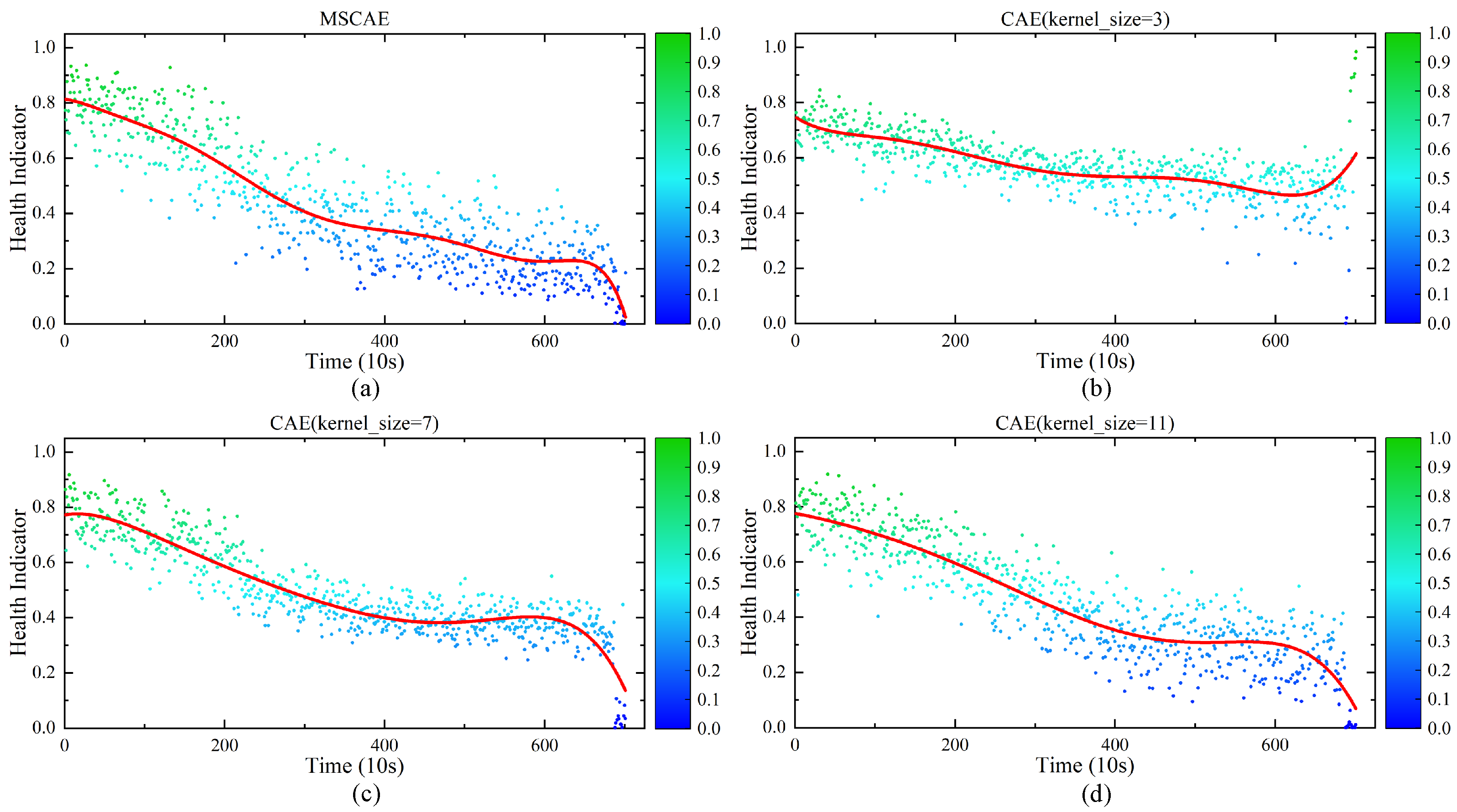
The HI obtained by MSCAE is compared with single-scale convolutional autoencoders with different convolutional kernel sizes, and the superiority of the proposed method is verified by a comprehensive evaluation index consisting of monotonicity, correlation and robustness.

(3)

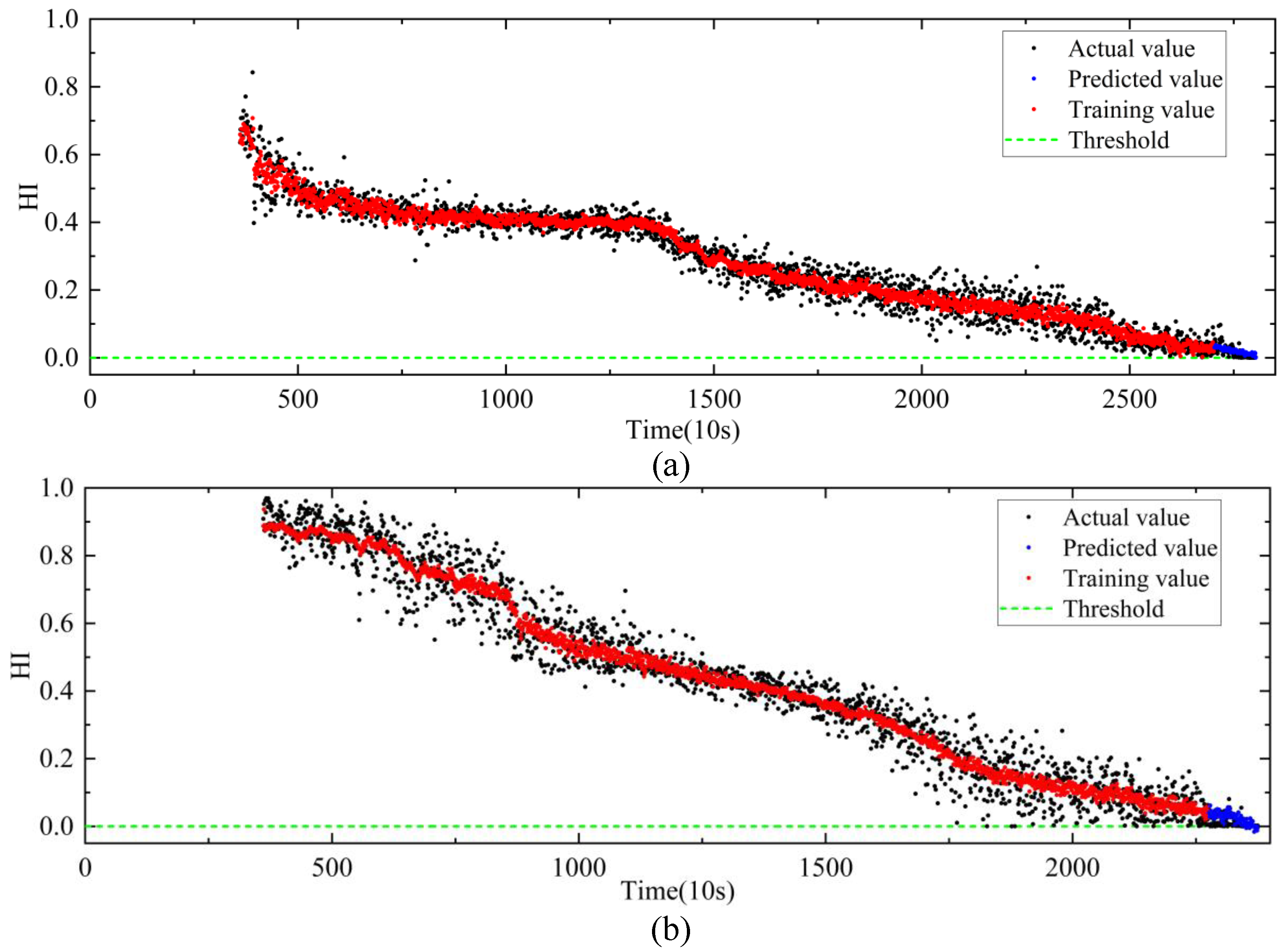
The HI obtained by MSCAE does not require artificial determination of the failure threshold, which is directly set to 0 and can be directly used for RUL prediction.

The remaining parts of this paper are organized as follows. Section 2 introduces the relevant theoretical knowledge covered in this paper. Section 3 presents the proposed HI construction method. Section 4 conducts relevant experiments and comparisons to verify the validity of the proposed method. Section 5 concludes this paper.

2. Related Theory

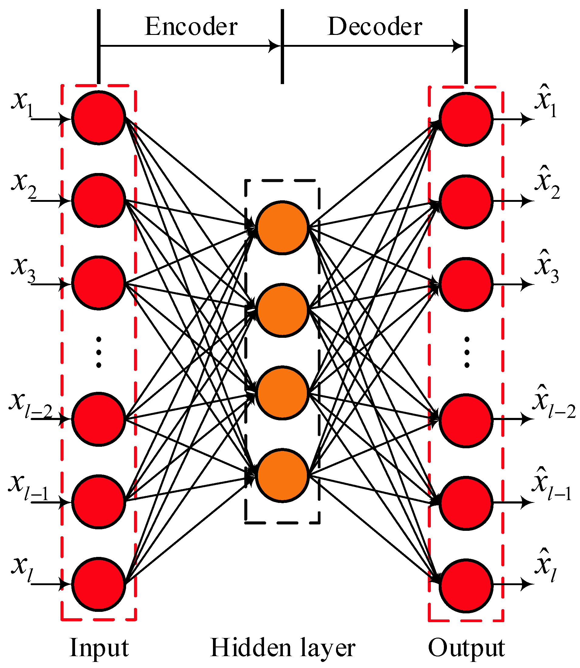
2.1. AE

AE was first proposed in the literature [29] as an unsupervised learning method and is often used for feature dimensionality reduction. AE consists of two parts: the encoder and the decoder. The encoder reduces the dimensionality of the input signals and extracts the high-level representations. The decoder takes the output results of the encoder as the input and reconstructs the input signals. AE uses a back-propagation algorithm to update the internal parameters to minimize the reconstruction error. The structure of a typical AE is shown in Figure 1.

Assume that the input of the encoder is $\mathit{x}=\left[x_1,x_2,\dots ,x_l\right]$. l is the length of the input data. Then, the output $\mathit{s}$ of the encoder can be expressed as:

$$\mathit{s}=f_e\left(W_e\mathit{x}+b_e\right)$$

(1)

where $W_e$ and $b_e$ denote the weight and bias, respectively, and $f_e$ denotes the encoder activation function. Then, the the decoder output $\widehat{\mathit{x}}=\left[{\widehat{x}}_1,{\widehat{x}}_2,\dots ,{\widehat{x}}_l\right]$ can be expressed as:

$$\widehat{\mathit{x}}=f_d\left(W_d\mathit{s}+b_d\right)$$

(2)

where $W_d$ and $b_d$ denote the weight and bias, respectively, and $f_d$ denotes the decoder activation function. The autoencoder optimizes the internal parameters by minimizing the reconfiguration error. The reconfiguration error $L_{AE}$ can be expressed as:

$$L_{AE}=\frac{1}{l}\sum _{i=1}^l{\left(x_i-{\widehat{x}}_i\right)}^2$$

(3)

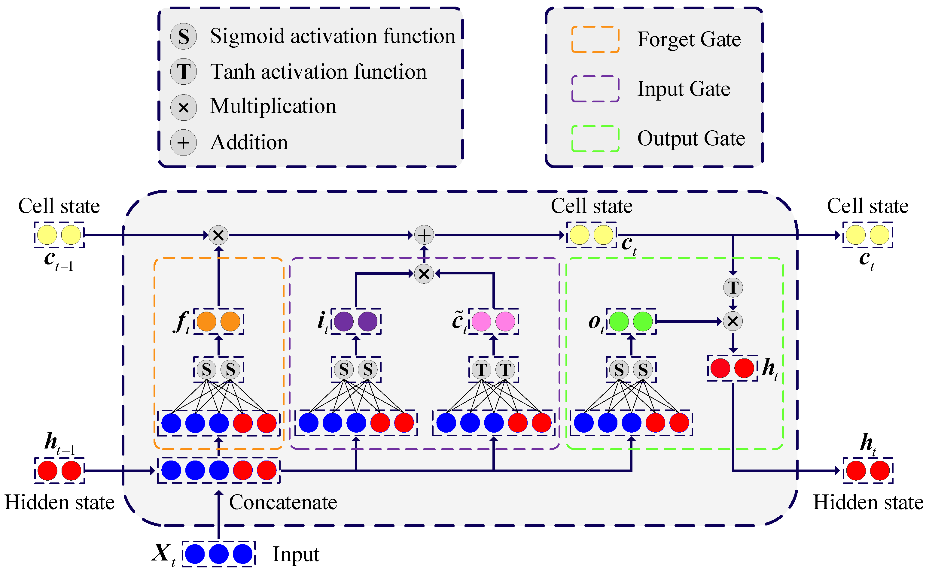
2.2. LSTM Neural Network

Data-driven methods for predicting the bearing RUL are usually based on monitoring data collected by sensors, such as temperature and vibration. There is a strong time dependence on these data. The recurrent neural network (RNN) model is characterized by taking sequence data as input and performing operations in the evolutionary direction of the sequence. Therefore, RNN can recognize time series and suit to solve RUL prediction problems. However, traditional RNN suffers from long-term dependency problems, and when training on long sequence data, gradient disappearance or gradient explosion may occur, resulting in ineffective training of the model. To solve this problem, Hochreiter and Schmidhuber proposed the LSTM model [30]. The structure of LSTM is shown in Figure 2. There are two information pathways in LSTM: one for storing long-term memory and one for short-term processing information and adding valid information to the other information pathway. In addition, three gating units, the input gate, forget gate and output gate, are added to the LSTM to control the information flow of input data in the LSTM unit. The formula of LSTM can be expressed as:

$$f_t=\sigma \left(W_f{x}_t+V_f{h}_{t-1}+b_f\right)$$

(4)

$$i_t=\sigma \left(W_i{x}_t+V_i{h}_{t-1}+b_i\right)$$

(5)

$${\tilde{c}}_t=tanh\left(W_c{x}_t+V_c{h}_{t-1}+b_c\right)$$

(6)

$$o_t=\sigma \left(W_o{x}_t+V_o{h}_{t-1}+b_o\right)$$

(7)

$$c_t=f_t\odot c_{t-1}+i_t\odot {\tilde{c}}_t$$

(8)

$$h_t=o_t\odot tanh\left(c_t\right)$$

(9)

where $x_t$ represents the input at moment t. $h_t$ and $c_t$ represent the hidden state and the cell state at the moment t, respectively. $f_t$ is the output of the forget gate. $i_t$ is the output of the input gate. $o_t$ is the output of the output gate. $W_f,V_f,W_i,V_i,W_c,V_c,W_o$, and $V_o$ represent the weight matrixes. $b_f,b_i,b_c$, and $b_o$ represent the bias matrixes. $\sigma$ and $tanh$ denote the sigmoid and hyperbolic tangent activation functions, respectively. ⊙ denotes point-by-point multiplication.

3. The Proposed Method

3.1. MSCAE

Based on the AE introduced in Section 2.1, the structure of the convolutional autoencoder is obtained by replacing the matrix operations in it with convolutional operations. Usually, features are extracted using convolutional kernels of the same size in the convolutional autoencoder. The literature [18] verified the effectiveness of the multi-scale convolutional network. Compared to traditional CNN, the use of parallel convolutional paths with different convolutional kernel sizes enables multi-scale learning, allowing the model to extract features from different time scales, ensuring the integrity of the representations and making full use of both global and local information. In this paper, we adopt the idea of multi-scale convolution to construct MSCAE to extract a more robust HI based on the full utilization of global and local degradation information, and the automatic extraction of HI can be realized. The structure of the proposed MSCAE is shown in Figure 3.

As shown in Figure 3, the proposed MSCAE uses three convolutional paths for feature extraction of the input data. It is worth noting that the three convolutional paths use one-dimensional convolution with different convolutional kernel sizes, aiming to make full use of the global and local information of the input data for more effective feature extraction.

In the encoding stage, three pathways perform parallel convolution and pooling operations on the input data. Suppose $E_{n,m}^i$ denotes the n-th channel of convolutional layer data in the m-th encode block in the i-th$(i=1,2,3)$ pathway and $N_m^e$ is the number of convolutional layer channels in the m-th encode block. Then, the one-dimensional convolution operation can be expressed as:

$$Z_{k,m+1}^{i,e}=f_r\left(\sum _{n=1}^{N_m^e}{E}_{n,m}^i\ast w_{k,n,m}^{i,e}+b_m^{i,e}\right)$$

(10)

where ∗ is the one-dimensional convolution operation. $w_{k,n,m}^{i,e}$ denotes the weight of the k-th convolutional kernel of the convolutional layer in the m-th encode block. $b_m^{i,e}$ is bias. $f_r$ adopts the ReLU activation function. $Z_{k,m+1}^{i,e}$ denotes the k-th channel data of the convolutional layer operation result in the m-th encode block of the i-th pathway.

After performing a convolution operation, a downsampling operation is performed on the convolution result using maximum pooling to reduce the size of the data. The pooling result $I_{k,m+1}^i$ for the k-th channel data of the pooling layer in the m-th encoding block of the i-th pathway can be expressed as:

$$E_{k,m+1}^i=P\left(Z_{k,m+1}^{i,e},p_m,s_m\right)$$

(11)

where P denotes the maximum pooling operation, $p_m$ is the size of the pooling window in the m-th convolution block, and $s_m$ is the stride. After the input data are extracted by L encoding blocks of features, the Flatten layer is used to turn the high-level representations into one-dimensional data, which is input to the fully connected block for HI extraction. It is worth noting that the fully connected block of MSCAE proposed in this paper uses only one fully connected layer in both encoding and decoding parts, and the number of hidden neurons is the same. Then, the extracted HI can be expressed as:

$$\widehat{y}=\sigma \left(W_{fe}{X}_e+b_{fe}\right)$$

(12)

where $\widehat{y}$ denotes the extracted HI, $W_{fe}$ and $b_{fe}$ denote the encoded partial weight and bias, respectively, and $\sigma$ denotes the Sigmoid activation function.

In the decoding stage, there are also three parallel paths. The decoding part in the fully connected block performs a dimensional expansion operation on the extracted HI, and the results obtained can be expressed as:

$$X_d=f_r\left(W_{fd}\widehat{y}+b_{fd}\right)$$

(13)

where $X_d$ denotes the output of the decoding part in the fully connected block, $W_{fd}$ and $b_{fd}$ denote the weight and bias of the decoding part in the fully connected block, respectively, and $f_r$ is the ReLU activation function. After obtaining $X_d$, it is dimensionally changed using the Reshape layer, and the transformed shape is the same as the shape of the input data in the Flatten layer. L decoding blocks reconstruct the results of the Reshape layer, i.e., three parallel upsampling and convolution pathways. Suppose $D_{n,m}^i$ denotes the n-th channel data of the upsampling layer in the m-th encoding block of the i-th$(i=1,2,3)$ pathway. Then, the operation of the upsampling layer can be expressed as:

$$Z_{n,m}^{i,d}=\mathrm{U}\left(D_{n,m}^i,u_m,{\mathrm{l}}_m\right)$$

(14)

where $Z_{n,m}^{i,d}$ is the result of the upsampling layer, U denotes the upsampling operation, and $u_m$ and $l_m$ represent the upsampling window size and stirde of the m-th decoding block, respectively. In a decoding block, the upsampling layer is connected after the convolution layer, and the convolution result of the m-th decoding block can be expressed as:

$$D_{k,m+1}^i=f_r\left(\sum _{n=1}^{N_m^d}{Z}_{n,m}^{i,d}\ast w_{k,n,m}^{i,d}+b_m^{i,d}\right)$$

(15)

where $D_{k,m+1}^i$ is the k-th channel data of the output of the m-th decoding block, $N_m^d$ denotes the total number of channels of the input data of the m-th decoding block, $w_{k,n,m}^{i,d}$ denotes the weight of the k-th convolutional kernel in the m-th decoding block, $b_m^{i,d}$ is the bias, and $f_r$ is the ReLU activation function. The reconstruction of the input data is obtained after processing by L decoding blocks. Assume that the i-th input data of MSCAE is ${\mathit{x}}_{\mathit{i}}=\left[x_{i,1},x_{i,2},\dots ,x_{i,l}\right]$, and the corresponding real RUL label is $y_i$, $i=1,2,\dots B$. l is the length of the input data, and B is the total life of the bearing. Then, the HI extracted by MSCAE is ${\widehat{y}}_i$, and the reconstruction of the input data is $\widehat{{\mathit{x}}_{\mathit{i}}}=\left[{\widehat{x}}_{i,1},{\widehat{x}}_{i,2},\dots {\widehat{x}}_{i,l}\right]$. In this paper, we use the composite loss function to evaluate the HI extraction capability of MSCAE. The composite loss consists of two parts: one is the error between the input data and the reconstructed data, and the other is the error between the HI and the true RUL. The composite loss function is calculated as follows.

$$J_{\theta }=\frac{1}{2}\sum _{i=1}^B{∥x_i-{\widehat{x}}_i∥}^2+\frac{\nu }{2}\sum _{i=1}^B{∥y_i-{\widehat{y}}_i∥}^2$$

(16)

where $\theta$ denotes the internal parameters of MSCAE and $\nu$ is a scaling factor to adjust the weight between the two errors. Compared with the traditional AE, the composite loss function constructed by MSCAE combines the supervised learning approach with the unsupervised learning approach for model training, which fully utilizes the degradation information of the bearings and enhances the extraction capability of the model HI. In the training phase of the model, the vibration data and labels of the training bearings are used to optimize the internal parameter $\theta$ using the back-propagation algorithm to minimize the composite loss. 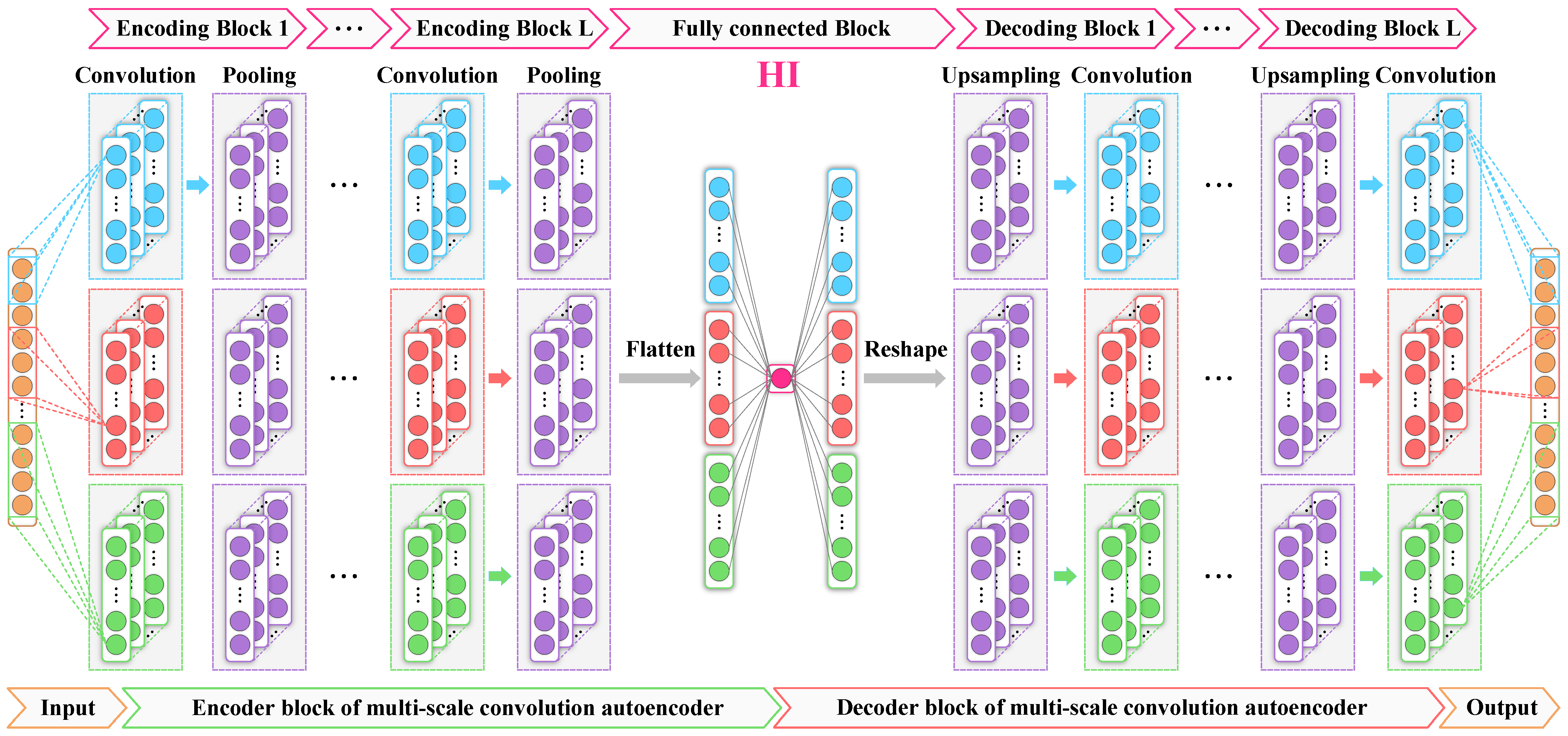In the testing phase of the model, the vibration data of the testing bearing serve as the input, and the HI is obtained using the encoder part of the trained MSCAE.

3.2. HI Extraction and RUL Prediction Process

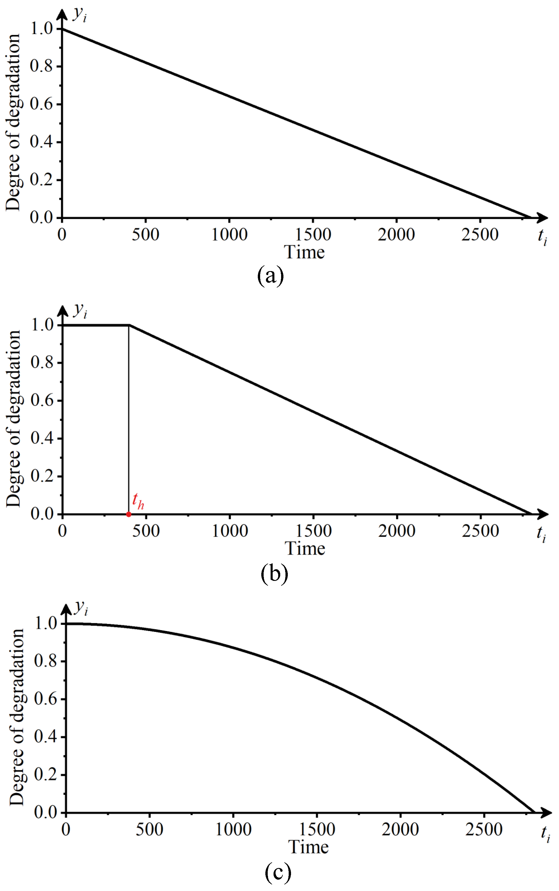
3.2.1. Construction Method of Degradation Labels

After obtaining the vibration data of the bearings, it is necessary to divide them into training and testing sets. Since the obtained original data do not have corresponding labels, it is necessary to construct the degradation labels corresponding to the vibration data. There are mainly two conventional methods for constructing degradation labels: linear degradation and segmental smoothing, and Figure 4 shows the differences between the two methods.

The degenerate label construction equation of Figure 4a can be expressed as

$$y_i=\frac{B-t_i}{B}$$

(17)

where B denotes the total life of the bearing, $t_i$ denotes the current time the bearing has been in operation, and $y_i$ denotes the current degradation level of the bearing. The degenerate label construction equation of Figure 4b can be expressed as:

$$y_i=\left\{\begin{array}{cc}1& \begin{array}{cc}if& t_i\le t_h\end{array}\\ 1-\frac{t_i-t_h}{B-t_h}& else\end{array}\right.$$

(18)

where $t_h$ indicates the degradation starting threshold; when $t_i$ is less than or equal to $t_h$, it is determined that the bearing has not started to degrade and the degradation label is always 1. When $t_h$ exceeds the threshold, it starts to show a linear degradation trend.

The first two methods of describing bearing degradation trends shown in Figure 4 have their own limitations compared to the true degradation of the bearing. The true bearing degradation does not exhibit a linear characteristic but rather degrades faster and faster as the operating time of the bearing increases. Therefore, the linear degradation method does not satisfy this operating characteristic. For the segmented smoothing method, the threshold $t_h$ at the degradation onset moment is usually determined artificially. However, $t_h$ is usually not the same for different operating conditions, and there are different bearings $t_h$ for the same operating conditions, which limits the application of the segmented smoothing method. The literature [31] proposed a method for constructing a degenerate trend based on a quadratic function, as shown in Figure 4c, and the specific expression can be expressed as:

$$y_i=1-\frac{t_i^2}{B^2}$$

(19)

The quadratic function-based method overcomes the shortcomings of the above two methods, and its constructed labels are more satisfying to the real degradation of the bearings. With the increase of the operation time, the degradation of the bearings is gradually accelerated, which is shown in Figure 4c as the slope of the curve gradually increases. Moreover, it is a convenient and effective method without artificially specifying the degradation threshold, so this paper adopts the quadratic function method to construct the degradation labels of bearings.

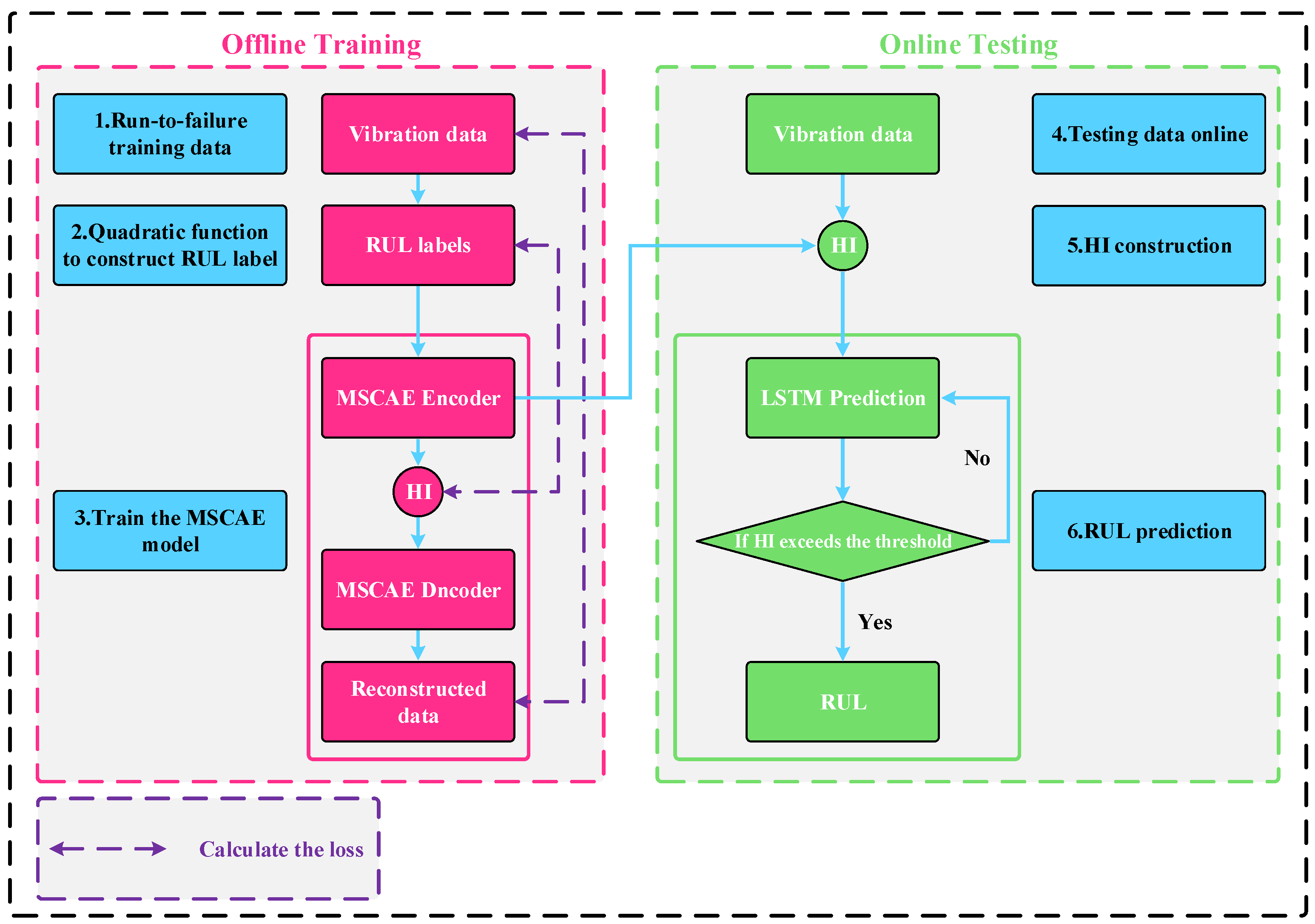
3.2.2. Overall Framework Flow

The overall framework flow of MSCAE-based HI extraction and RUL prediction proposed in this paper is shown in Figure 5. The framework is divided into two main phases, offline training and online testing. There are three main steps in the offline training phase, and the process is as follows.

• Vibration data from training bearing operation to failure are obtained using vibration sensors. Suppose the vibration data are $X=\left[{\mathit{x}}_{\mathbf{1}},{\mathit{x}}_{\mathbf{2}},\dots ,{\mathit{x}}_{\mathit{B}}\right]$, ${\mathit{x}}_{\mathit{i}}=\left[x_{i,1},x_{i,2},\dots ,x_{i,l}\right]$, ${\mathit{x}}_{\mathit{i}}$ represents the vibration data at the moment $t_i$, $i=1,2,\dots B$, B is the total time of bearing operation, and l is the length of the data.
• The degenerate labels for each moment of the vibration data are calculated using Equation (19), and the labels $\mathit{y}=\left[y_1,y_2,\dots y_B\right]$ are obtained by the calculation.
• Training the proposed MSCAE model. First, the vibration datum X of the training bearing is input to the model, and the output of the MSCAE encoding part is the extracted HI, which is denoted as $\widehat{\mathit{y}}=\left[{\widehat{y}}_1,{\widehat{y}}_2,\dots {\widehat{y}}_B\right]$. After that, HI is used as an input to the decoding part of MSCAE to obtain the reconstructed data $\widehat{X}=\left[{\widehat{\mathit{x}}}_{\mathbf{1}},{\widehat{\mathit{x}}}_{\mathbf{2}},\dots ,{\widehat{\mathit{x}}}_{\mathit{B}}\right]$ of the vibration data X. Finally, the composite loss function is calculated using Equation (16), and the internal parameters $\theta$ of the model are updated using the back-propagation algorithm. After the MSCAE is trained offline, it moves to the online testing phase.
• The vibration data from test bearing operation to failure are obtained, which are defined as $X^{\prime }=\left[{{\mathit{x}}^{\mathbf{\prime }}}_{\mathbf{1}},{{\mathit{x}}^{\mathbf{\prime }}}_{\mathbf{2}},\mathbf{\dots }{{\mathit{x}}^{\mathbf{\prime }}}_{\mathit{T}}\right]$, and T is the total operating time of the testing bearing.
• The vibration signal $X^{\prime }$ of the testing bearing is input to the encoder of the MSCAE trained in step 3 to obtain in HI $\mathit{H}=\left[h_1,h_2,\dots h_T\right]$ of the test bearing.
• After obtaining the HI of the testing bearing, the first N points of $\mathit{H}$ are taken to construct the training data for training the LSTM model. The training matrix can be expressed as follows.

  $$\mathit{V}=\left[\begin{array}{cccc}{h}_1& h_2& \cdots & h_{N-M}\\ h_2& h_3& \cdots & h_{N-M+1}\\ ⋮& ⋮& \ddots & ⋮\\ h_{M+1}& h_{M+2}& \cdots & h_N\end{array}\right]=\left[\begin{array}{c}{\mathbf{\nu }}_{\mathbf{1}}\\ {\mathbf{\nu }}_{\mathbf{2}}\\ ⋮\\ {\mathbf{\nu }}_{\mathit{M}+\mathbf{1}}\end{array}\right]$$

  (20)

  where M is the neurons number of the LSTM output layer, ${\mathbf{\nu }}_{\mathit{i}}=\left[h_i,h_{i+1},\dots ,h_{i+N-M-1}\right],$$(i=[1,2,\dots ,M+1\left]\right)$. The LSTM is trained by taking the first M vectors of the training matrix $\mathit{V}$ as the input of the LSTM and the last vector ${\mathit{\nu }}_{\mathit{M}+\mathbf{1}}$ as the output. Assuming that the mapping function of the trained LSTM is denoted as f, the last M vectors of the matrix $\mathit{V}$ are passed as input to the trained LSTM to obtain the first prediction result ${\overline{\mathbf{\nu }}}_{\mathit{M}+\mathbf{2}}$, and the specific expression is:

  $${\overline{\mathbf{\nu }}}_{\mathit{M}+\mathbf{2}}=f\left(\left[{\mathbf{\nu }}_{\mathbf{2}},{\mathbf{\nu }}_{\mathbf{3}},\cdots ,{\mathbf{\nu }}_{\mathit{M}+\mathbf{1}}\right]\right)$$

  (21)
  Then, the matrix $\mathit{V}$ can be updated as follows:

  $$\mathit{V}={\left[{\mathbf{\nu }}_{\mathbf{1}},{\mathbf{\nu }}_{\mathbf{2}},\cdots ,{\mathbf{\nu }}_{\mathit{M}+\mathbf{1}},{\overline{\mathbf{\nu }}}_{\mathit{M}+\mathbf{2}}\right]}^T$$

  (22)

The above method allows the prediction of HI vectors to be performed continuously and the matrix $\mathit{V}$ to be continuously updated. Thus, ${\overline{\mathbf{\nu }}}_{\mathit{k}}$ can be expressed as:

$${\overline{\mathbf{\nu }}}_{\mathit{k}}=f\left(\left[{\mathbf{\nu }}_{\mathit{M}-\mathit{k}},{\mathbf{\nu }}_{\mathit{M}+\mathbf{1}},\dots ,{\overline{\mathbf{\nu }}}_{\mathit{M}+\mathbf{2}},\dots ,{\overline{\mathbf{\nu }}}_{\mathit{M}+(\mathit{k}-\mathit{M}-\mathbf{1})}\right]\right)$$

(23)

Meanwhile, the matrix $\mathit{V}$ is updated as follows:

$$\mathit{V}={\left[{\mathbf{\nu }}_{\mathbf{1}},\dots ,{\mathbf{\nu }}_{\mathit{M}+\mathbf{1}},{\overline{\mathbf{\nu }}}_{\mathit{M}+\mathbf{2}},\dots ,{\overline{\mathbf{\nu }}}_{\mathit{k}}\right]}^T$$

(24)

where ${\overline{\mathbf{\nu }}}_{\mathit{k}}=\left[h_k,\dots ,h_N,{\overline{h}}_{N+1},\dots ,{\overline{h}}_{k+N-M-1}\right]$. When ${\overline{h}}_{k+N-M-1}$ is less than the threshold 0, the prediction step is stopped, and the RUL of the bearing is obtained as $(k-M)\times T_s$, and $T_s$ is the sampling interval of the vibration sensor. If the prediction result is not less than the threshold, the iterative prediction is continued until the predicted value is less than the threshold and the corresponding RUL is obtained.

4. Experimental Analysis

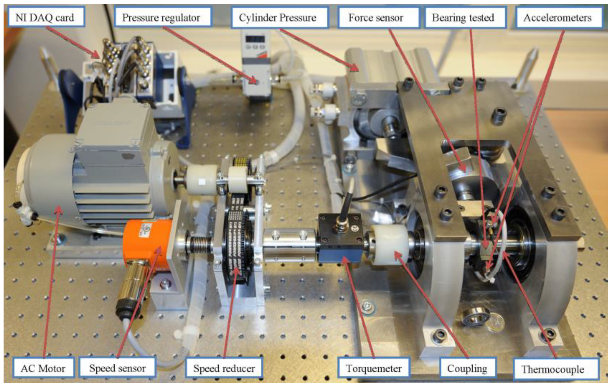
4.1. Data Introduction

The experimental data in this paper were obtained from the PHM Challenge [32] organized by the Institute of Electrical and Electronics Engineers in 2012, and the data were obtained from the PRONOSTIA experimental bench, as shown in Figure 6. The experimental bench consists of three main parts: the rotation part, the degradation generation part and the sensor part. The rotating part consists of an asynchronous motor with a gearbox and two shafts to provide the working environment for the test bearing. The degradation generating part can apply radial load to the testing bearing to simulate the actual working operation with load and accelerate the degradation, which can complete the whole process of bearing operation to failure in a short time. The sensor part consists of three sensors, two of which are vibration sensors positioned 90° apart, measuring the magnitude of horizontal and radial vibrations, respectively, and the other is a temperature sensor, measuring the temperature of the bearing during operation.

The PHM2012 challenge data give the full cycle life data of the bearings from operation to failure for three operating conditions. The three operating conditions are 1800 rpm and 4000 N; 1650 rpm and 4200 N; and 1500 rpm and 5000 N. There are 7, 7, 3 test bearings for each of the three operating conditions. The PRONOSTIA test bench has a sampling interval of 10 s, a sampling duration of 0.1 s, and a sampling frequency of 25.6 kHz, indicating that every 10 s, the sensor can collect 2560 data points.

In order to verify the effectiveness of the MSCAE proposed in this paper, the data set needs to be divided into training data and testing data. The division method in this paper is shown in

Table 1. Training set and test set division.

	Training Set	Test Set
Condition 1	Bearing1_2 Bearing1_4 Bearing1_5 Bearing1_6 Bearing1_7	Bearing1_1 Bearing1_3
Condition 2	Bearing2_1 Bearing2_2 Bearing2_3 Bearing2_4 Bearing2_5 Bearing2_7	Bearing2_6
Condition 3	Bearing3_1 Bearing3_2	Bearing3_3

. As can be seen from Table 1, all bearings under three operating conditions are used in this paper to validate the proposed method. The training set contains 5, 6, 2 bearings, and the testing set contains 2, 1, 1 bearings.

4.2. Evaluation Metrics

To verify the effectiveness of the proposed MSCAE to extract HI in this paper, three evaluation metrics, monotonicity, correlation and robustness, were used to quantify the performance of HI [31]. It is worth noting that the range of all three metrics is within [0, 1].

• Monotonicity: It aims to assess the tendency of HI to increase monotonically or decrease monotonically as the running time increases. The stronger the monotonicity of HI, the closer it is to 1. The specific formula for monotonicity can be expressed as:

  $$Mon\left(H\right)=\left|\frac{\mathrm{No}.\mathrm{of}dH>0}{T-1}-\frac{\mathrm{No}.\mathrm{of}dH<0}{T-1}\right|$$

  (25)

  where $dH$ denotes the first-order derivative between two HI values and T denotes the number of HI and also the number of sensor samples.
• Correlation: It aims to measure the correlation between HI and runtime. The more correlated the two are, the closer the value of correlation is to 1, and vice versa. The formula for correlation can be expressed as:

  $$Corr\left(H\right)=\frac{\left|{\displaystyle \sum _{i=1}^T}\left(h_i-\overline{H}\right)\left(t_i-\overline{T}\right)\right|}{\sqrt{{\displaystyle \sum _{i=1}^T}{\left(h_i-\overline{H}\right)}^2{\displaystyle \sum _{i=1}^T}{\left(t_i-\overline{T}\right)}^2}}$$

  (26)

  where $\overline{H}={\sum }_{i=1}^T{h}_i/T$ and $\overline{T}={\sum }_{i=1}^T{t}_i/T$.
• Robustness: It aims to measure the ability of HI to resist outlier interference; the stronger its ability, the closer the robustness is to 1, and vice versa. The extracted HI can be seen as a superposition of the average trend and noise, whereby H can be expressed as:

  $$H\left(t_i\right)=H_T\left(t_i\right)+H_R\left(t_i\right)$$

  (27)

  where $H_T\left(t_i\right)$ denotes the average trend of HI at the moment T, and $H_R\left(t_i\right)$ denotes the noise disturbance of HI at the moment T. Then, the robustness is calculated by the formula:

  $$Rob\left(H\right)=\frac{1}{T}\sum _{i=1}^{T}exp\left(-\left|\frac{H_R\left(t_i\right)}{H\left(t_i\right)}\right|\right)$$

  (28)

In order to comprehensively evaluate the advantages and disadvantages of the extracting HI, a Composite Indicator (CI) containing the above three indicators is proposed, which is defined as:

$$\mathrm{CI}=\frac{1}{3}\left(\mathrm{Mon}+\mathrm{Corr}+\mathrm{Rob}\right)$$

(29)

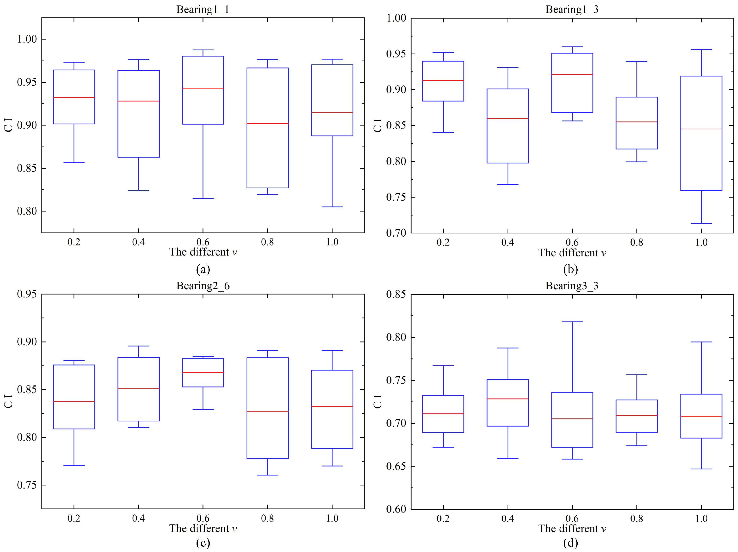
4.3. The Validity of MSCAE

The specific structure of the MSCAE proposed in this paper is shown in Figure 7. As can be seen from Figure 7, MSCAE consists of three encoding blocks, three decoding blocks and one fully connected block. The number of convolutional kernels in the three coding blocks is 8, 16, 4, and the size of convolutional kernels in the three pathways is 3 × 1, 7 × 1 and 11 × 1, respectively, and the size and stride of maximum pooling are 8. The number of convolutional kernels in the three decoding blocks is 16, 8, 1, and the size of convolutional kernels in the three pathways is the same as the decoder, and the size and stride of upsampling are 8. The Sigmoid activation function is used in the fully connected block when the second layer obtains HI. The activation function is not used when reconstructed data are obtained. All the remaining layers use the ReLU activation function, and each layer uses the BatchNormalization (BN) layer to improve the model generalization. The detailed hyperparameter settings of the model are shown in

Table 2. Hyperparameter setting of the model.

Hyperparameter	Value
Batch size	128
Epoch	100
Learning rate $lr$	Adam (0.0001)
Number of Encoding Block	3
Number of Decoding Block	3
Kernel size	$\left[3\times 1\right],\left[7\times 1\right],\left[11\times 1\right]$
Pooling size	8
Upsampling size	8
Number of fully connected layer units	$\left[60,1,60\right]$

. Comparative experiments are conducted in this paper to choose the scale factor v of the composite loss function. In this paper, five values of 0.2, 0.4, 0.6, 0.8 and 1.0 are selected for comparison and validation. Ten experiments are conducted on four test bearings using these five values, respectively, and the final box line diagram is obtained, as shown in Figure 8. From Figure 8, it can be seen that v is taken as 0.6, 0.6 and 0.4, respectively, as the best choice for the three working conditions.

After training the MSCAE using the training bearing data, the MSCAE was tested using testing bearings, and the HI extracted by four testing bearings is shown in Figure 9. In Figure 9, the green color indicates that the value of HI is closer to 1, and the blue color is closer to 0. The red curve is the HI trend curve fitted using polynomials. Four bearings in Figure 9 have a clear downward trend in HI, and by the time sampling stops, the value of HI is close to 0.

In order to verify the superiority of MSCAE, this paper sets up a comparison between MSCAE and three convolutional autoencoders (CAE) with constant convolutional kernel sizes of $3\times 1$, $7\times 1$ and $11\times 1$, respectively. To ensure the completeness of the experiments, the structure of the CAE is the same as the structure of a pathway in MSCAE. Moreover, when the model is trained, the hyperparameters are set the same as MSCAE. The obtained results are shown in Figure 10. From Figure 10, it can be seen that MSCAE exceeds the other three models in CI for the tested bearings under each operating condition. It shows that MSCAE can combine the advantages of different convolutional kernel sizes to identify different time scale information and make full use of the local and global information of the original vibration signal to extract a more effective HI. To further verify the superiority of MSCAE, four models were used to extract the HI of Bearing$2\_6$ bearing for analysis, as shown in Figure 11. When the convolution kernel size is set to 3, the final HI trend increases, which is against the degradation law of the real bearing. Moreover, when the convolution kernel size is 7 and 11, the final HI trend decreases to 0. However, both undergo abrupt changes when the bearing is damaged, i.e., the HI value directly decreases to 0. The abrupt change is most obvious when the convolution kernel size is 7, and this phenomenon affects the prediction of RUL. Therefore, it is desired to obtain an HI that can satisfy the real degradation trend of the bearing, and the degradation process of the HI is relatively flat, which is conducive to the continuous prediction of RUL. It can be found that the HI extracted by MSCAE proposed in this paper can meet the above requirements.

4.4. RUL Prediction

After extracting the HI of the testing bearing using MSCAE, it can be found that the extracted HI has obvious degradation characteristics with time, which indicates that the HI is a time series. Therefore, LSTM is used to perform the RUL prediction of bearings. For Bearing$1\_1$, assuming that the last 100 HI are unknown and the first 2703 HI are known, the known 2703 HI points are used as training data for the LSTM to predict the unknown HI points, and when the predicted value of the LSTM is less than the threshold 0, it means that the predicted current moment bearing has been damaged, and the time interval between the current moment and the starting moment of the prediction is the predicted RUL value. Similarly, for Bearing$1\_3$, assuming that the last 100 HI points are unknown, the training data for the LSTM are the first 2275 HI points. The parameters of the LSTM are configured as shown in

Table 3. Hyperparameter configuration of LSTM.

Parameters	Value
The number of neurons in the input layer	360
The number of neurons in the hidden layer	29
The number of neurons in the output layer	1
Learning rate $lr$	0.07
Optimizer	Adam

. The number of neurons in the input, hidden, and output layers of the LSTM are 360.29 and 1, respectively. The internal parameters of the LSTM are optimized using the Adam optimizer, and the learning rate is set to 0.07.

To demonstrate the superiority of the HI extraction method proposed in this paper on RUL prediction, two state-of-the-art deep learning-based HI construction methods are used for comparison. One is the recurrent convolutional neural network (RCNN), which was proposed in the literature [33], and the other is the CNN proposed in the literature [25]. The RCNN is an end-to-end HI extraction framework consisting of a convolutional neural network with residual structure and an LSTM serially connected with the specific structural parameters described in the literature [33]. The CNN-based HI construction method proposed in the literature [25] is divided into two steps, first using two convolutional layers for feature extraction and later using a fully connected layer for HI construction. It is worth noting that both methods, as in this paper, use the original vibration signal as the input to the model without a manual feature extraction step. All three methods are trained using the same training data, and the RUL prediction ability of the extracted HI is verified on Bearing$1\_1$ and Bearing$1\_3$. For convenience, the HI extracted by the proposed MSCAE, RCNN and CNN are MSCAE-HI, CRNN-HI and CNN-HI.

The RUL prediction results of HI extracted by the three models are shown in Figure 12, Figure 13 and Figure 14. From Figure 13, it can be found that RUL prediction using CRNN-HI requires artificially set thresholds, and the choice of thresholds directly affects the RUL prediction results. If the set threshold is large, it will cause the prediction to stop early, and conversely, it will cause the prediction value of RUL to be larger than the real one, or even the phenomenon that it cannot converge to the set threshold. In this paper, the failure threshold of CRNN-HI is set to 0.2. In Figure 13a, the HI of Bearing$1\_1$ extracted using the CRNN method shows an increasing trend at the end of degradation, which deviates from the actual degradation threshold and can affect the prediction ability of the LSTM. In Figure 13b, there are a few outliers in the HI of Bearing$1\_3$, and there are HI points less than the threshold value when the bearing first starts running. It can be found in Figure 14 that there is a significant divergence of CNN-HI at the late degradation stage of the bearing, resulting in the predicted HI value being more likely to be close to the failure threshold when using CNN-HI for RUL prediction, resulting in the predicted RUL often being smaller than the true RUL value. In Figure 12, the MSCAE-HI constructed in this paper has less fluctuation and a smoother degradation trend, which can effectively reflect the real degradation trend of the bearing. Using MSCAE-HI for RUL prediction, the predicted RUL results are closer to the true values, and the predicted HI is more consistent with the true degradation trend. Combining the above analysis, the MSCAE-HI method proposed in this paper is more suitable for the RUL prediction of bearings.

To further validate the superiority of MSCAE-HI, five metrics for evaluating the prediction accuracy of RUL were used to compare the prediction performance of the three methods. These five evaluation metrics are score scoring function, mean absolute error (MAE), normalized root mean square error (NRMSE), root mean square error (RMSE) and mean absolute percentage error (MAPE), which are defined in the literature [23]. Three methods were used to conduct five prediction experiments for Bearing$1\_1$ and Bearing$1\_3$, and the final evaluation results are shown in

Table 4. Results of RUL prediction evaluation for 3 HI.

		Score
	MSCAE-HI	CRNN-HI	CNN-HI
Bearing1_1	$\mathbf{0.3315}$	0.2334	0.1379
Bearing1_3	$\mathbf{0.4979}$	0.1366	0.0712
		MAE
	MSCAE-HI	CRNN-HI	CNN-HI
Bearing1_1	$\mathbf{152}$	276	602
Bearing1_3	$\mathbf{214}$	356	808
		NRMSE
	MSCAE-HI	CRNN-HI	CNN-HI
Bearing1_1	$\mathbf{0.1516}$	0.2601	1.5480
Bearing1_3	$\mathbf{0.2938}$	0.3596	4.2882
		RMSE
	MSCAE-HI	CRNN-HI	CNN-HI
Bearing1_1	$\mathbf{160.13}$	296.58	616.13
Bearing1_3	$\mathbf{230.95}$	378.31	823.33
		MAPE
	MSCAE-HI	CRNN-HI	CNN-HI
Bearing1_1	$\mathbf{15.2}$	27.6	60.2
Bearing1_3	$\mathbf{21.4}$	35.6	80.8

. In Table 4, the MAE, NRMSE, RMSE and MAPE of CNN-HI are the maximum among three methods. This phenomenon can be explained that the fluctuation of CNN-HI is very obvious at the late degradation stage, and the HI predicted by the LSTM is easily smaller than the degradation threshold, resulting in a large deviation of the predicted from the true RUL. RUL prediction using MSCAE-HI obtained the maximum score values and the minimum MAE, MRMSE, RMSE, and MAPE values on both Bearing$1\_1$ and Bearing$1\_3$, which once again confirmed the superiority of the HI indicator extraction method of MSCAE proposed in this paper.

5. Conclusions

In this paper, a novel framework for HI extraction, called MSCAE, is proposed. It can overcome the disadvantages of traditional methods that require manual extraction of time-frequency domain indicators as features and the need to set failure thresholds by experience in RUL prediction. It relies solely on the raw sensor vibration signal to extract HI and does not require additional determination of the failure threshold. MSCAE can use convolutional kernels of different sizes to effectively exploit the global and local information of vibration signals, enhancing the HI extraction capability. A quadratic function-based label is first constructed for the original vibration data, after which the model is trained using the training data, and the internal parameters are optimized using a compound loss function. Then, HI is extracted using the test-bearing data to verify the validity of MSCAE. Finally, the RUL prediction is performed using LSTM. The HI extraction capability of MSCAE is verified to be superior to that of CAE models using a single scale with the PHM2012 dataset. Furthermore, it is compared with two state-of-the-art HI construction methods, CRNN and CNN, to judge the prediction performance of RUL using five evaluation metrics. The comparison results confirm the superiority of the proposed MSCAE-extracted HI for RUL prediction. In this paper, HI extraction and RUL prediction for rolling bearings achieved excellent results; however, the generalization capability for mechanical components such as gears and engines needs further validation. The future direction is to apply MSCAE to HI extraction and RUL prediction of other mechanical components.

References

- Ren, L.; Cui, J.; Sun, Y.; Cheng, X. Multi-bearing remaining useful life collaborative prediction: A deep learning approach. J. Manuf. Syst. 2017, 43, 248–256. [Google Scholar] [CrossRef]
- Pan, Z.; Meng, Z.; Chen, Z.; Gao, W.; Shi, Y. A two-stage method based on extreme learning machine for predicting the remaining useful life of rolling-element bearings. Mech. Syst. Signal Process. 2020, 144, 106899. [Google Scholar] [CrossRef]
- Gao, S.; Han, Q.; Zhou, N.; Pennacchi, P.; Chatterton, S.; Qing, T.; Zhang, J.; Chu, F. Experimental and theoretical approaches for determining cage motion dynamic characteristics of angular contact ball bearings considering whirling and overall skidding behaviors. Mech. Syst. Signal Process. 2022, 168, 108704. [Google Scholar] [CrossRef]
- Ambrożkiewicz, B.; Syta, A.; Gassner, A.; Georgiadis, A.; Litak, G.; Meier, N. The influence of the radial internal clearance on the dynamic response of self-aligning ball bearings. Mech. Syst. Signal Process. 2022, 171, 108954. [Google Scholar] [CrossRef]
- Zhang, Y.; Wang, J.; Du, H.; Yin, P. Error Evaluation of the Crown Profile of Logarithmic Generatrix Roller. J. Phys. Conf. Ser. 2021, 1948, 012065. [Google Scholar] [CrossRef]
- Zhu, J.; Chen, N.; Peng, W. Estimation of Bearing Remaining Useful Life Based on Multiscale Convolutional Neural Network. IEEE Trans. Ind. Electron. 2019, 66, 3208–3216. [Google Scholar] [CrossRef]
- Zhao, H.; Liu, H.; Jin, Y.; Dang, X.; Deng, W. Feature Extraction for Data-driven Remaining Useful Life Prediction of Rolling Bearings. IEEE Trans. Instrum. Meas. 2021, 70, 1–10. [Google Scholar] [CrossRef]
- Deng, K.; Zhang, X.; Cheng, Y.; Zheng, Z.; Peng, J. A remaining useful life prediction method with long-short term feature processing for aircraft engines. Appl. Soft Comput. 2020, 93, 106344. [Google Scholar] [CrossRef]
- Xiang, S.; Qin, Y.; Luo, J.; Pu, H.; Tang, B. Multicellular LSTM-based deep learning model for aero-engine remaining useful life prediction. Reliab. Eng. Syst. Saf. 2021, 216, 107927. [Google Scholar] [CrossRef]
- Zeng, F.; Li, Y.; Jiang, Y.; Song, G. A deep attention residual neural network-based remaining useful life prediction of machinery. Measurement 2021, 181, 109642. [Google Scholar] [CrossRef]
- Song, Y.; Gao, S.; Li, Y.; Jia, L.; Pang, F. Distributed Attention-Based Temporal Convolutional Network for Remaining Useful Life Prediction. IEEE Internet Things J. 2020, 8, 9594–9602. [Google Scholar] [CrossRef]
- Chen, Z.; Wu, M.; Zhao, R.; Guretno, F.; Li, X. Machine Remaining Useful Life Prediction via an Attention Based Deep Learning Approach. IEEE Trans. Ind. Electron. 2020, 68, 2521–2531. [Google Scholar] [CrossRef]
- Que, Z.; Jin, X.; Xu, Z. Remaining Useful Life Prediction for Bearings Based on a Gated Recurrent Unit. IEEE Trans. Instrum. Meas. 2021, 70, 1–11. [Google Scholar] [CrossRef]
- Meng, Z.; Li, J.; Yin, N.; Pan, Z. Remaining useful life prediction of rolling bearing using fractal theory. Measurement 2020, 156, 107572. [Google Scholar] [CrossRef]
- Wang, B.; Lei, Y.; Li, N.; Li, N. A Hybrid Prognostics Approach for Estimating Remaining Useful Life of Rolling Element Bearings. IEEE Trans. Reliab. 2018, 69, 1–12. [Google Scholar] [CrossRef]
- Ren, L.; Sun, Y.; Cui, J.; Zhang, L. Bearing remaining useful life prediction based on deep autoencoder and deep neural networks. J. Manuf. Syst. 2018, 48, 71–77. [Google Scholar] [CrossRef]
- Liu, L.; Song, X.; Chen, K.; Hou, B.; Ning, H. An enhanced encoder–decoder framework for bearing remaining useful life prediction. Measurement 2020, 170, 108753. [Google Scholar] [CrossRef]
- Wang, B.; Lei, Y.; Li, N.; Wang, W. Multi-Scale Convolutional Attention Network for Predicting Remaining Useful Life of Machinery. IEEE Trans. Ind. Electron. 2020, 68, 7496–7504. [Google Scholar] [CrossRef]
- Meng, M.; Zhu, M. Deep Convolution-based LSTM Network for Remaining Useful Life Prediction. IEEE Trans. Ind. Inform. 2020, 17, 1658–1667. [Google Scholar]
- Cao, Y.; Ding, Y.; Jia, M.; Tian, R. A novel temporal convolutional network with residual self-attention mechanism for remaining useful life prediction of rolling bearings. Reliab. Eng. Syst. Saf. 2021, 215, 107813. [Google Scholar] [CrossRef]
- Yao, D.; Li, B.; Liu, H.; Yang, J.; Jia, L. Remaining useful life prediction of roller bearings based on improved 1D-CNN and simple recurrent unit. Measurement 2021, 175, 109166. [Google Scholar] [CrossRef]
- Hai, Q.; Lee, J.; Jing, L.; Gang, Y. Robust performance degradation assessment methods for enhanced rolling element bearing prognostics. Adv. Eng. Inform. 2003, 17, 127–140. [Google Scholar]
- Qin, Y.; Chen, D.; Xiang, S.; Zhu, C. Gated Dual Attention Unit Neural Networks for Remaining Useful Life Prediction of Rolling Bearings. IEEE Trans. Ind. Inform. 2021, 17, 6438–6447. [Google Scholar] [CrossRef]
- Chen, Y.; Peng, G.; Zhu, Z.; Li, S. A novel deep learning method based on attention mechanism for bearing remaining useful life prediction. Appl. Soft Comput. 2019, 86, 105919. [Google Scholar] [CrossRef]
- Guo, L.; Lei, Y.; Li, N.; Yan, T.; Li, N. Machinery health indicator construction based on convolutional neural networks considering trend burr. Neurocomputing 2018, 292, 142–150. [Google Scholar] [CrossRef]
- Li, N.; Lei, Y.; Lin, J.; Ding, S.X. An Improved Exponential Model for Predicting Remaining Useful Life of Rolling Element Bearings. IEEE Trans. Ind. Electron. 2015, 62, 7762–7773. [Google Scholar] [CrossRef]
- Guo, L.; Li, N.; Jia, F.; Lei, Y.; Lin, J. A recurrent neural network based health indicator for remaining useful life prediction of bearings. Neurocomputing 2017, 240, 98–109. [Google Scholar] [CrossRef]
- Chen, D.; Qin, Y.; Luo, J.; Xiang, S. Gated Adaptive Hierarchical Attention Unit Neural Networks for the Life Prediction of Servo Motors. IEEE Trans. Ind. Electron. 2022, 69, 9451–9461. [Google Scholar] [CrossRef]
- Rumelhart, D.E.; McClelland, J.L. Learning Internal Representations by Error Propagation. In Parallel Distributed Processing: Explorations in the Microstructure of Cognition: Foundations; MIT Press: Cambridge, MA, USA, 1987; pp. 318–362. [Google Scholar]
- Hochreiter, S.; Schmidhuber, J. Long Short-Term Memory. Neural Comput. 1997, 9, 1735–1780. [Google Scholar] [CrossRef]
- Chen, D.; Qin, Y.; Wang, Y.; Zhou, J. Health indicator construction by quadratic function-based deep convolutional auto-encoder and its application into bearing RUL prediction. ISA Trans. 2021, 114, 44–56. [Google Scholar] [CrossRef]
- Nectoux, P.; Gouriveau, R.; Medjaher, K.; Ramasso, E.; Varnier, C. PRONOSTIA: An experimental platform for bearings accelerated degradation tests. In Proceedings of the IEEE International Conference on Prognostics and Health Management, San Francisco, CA, USA, 17–20 June 2012. [Google Scholar]
- Chen, L.; Xu, G.; Zhang, S.; Yan, W.; Wu, Q. Health indicator construction of machinery based on end-to-end trainable convolution recurrent neural networks. J. Manuf. Syst. 2020, 54, 1–11. [Google Scholar] [CrossRef]