Water Surface and Ground Control of a Small Cross-Domain Robot Based on Fast Line-of-Sight Algorithm and Adaptive Sliding Mode Integral Barrier Control

Abstract

This paper focuses on the control method of small cross-domain robots (CDR) on the water surface and the ground. The maximum size of the robot is 85 cm and the weight of the robot is 6.5 kg. To solve the problem that CDRs cannot handle the lateral velocity, which leads to error in tracking the desired trajectory, a fast line of sight (FLOS) algorithm is proposed. In this method, an exponential term is introduced to plan the yaw angle, and a fast-extended state observer (FESO) is designed to observe the side slip angle without small angle assumption. The performances and working environments of CDRs are different on the ground and the water surface. Therefore, to avoid the driver saturation and putting risk, an adaptive sliding mode integral barrier control (ASMIBC) is proposed to constrain the robot state. This control method solves the constraint failure of the traditional integral barrier control (IBC) when the desired state is a constant. The gain of the sliding mode is adaptively adjusted by the error between the limit state and the actual state. In addition, the adaptive rate is designed for uncertain time-varying lumped disturbances, such as water resistance, currents and wind. Simulation results demonstrate the effectiveness of the proposed control method.

1. Introduction

Multi-habitat robots have been widely studied in recent years. Those robots can be divided into land–air robots and amphibious robots according to the environments of their working. For the land–air robots, quadrotors are often adopted, because of the advantages of simple structure, vertical take-off and landing, and easy maintenance. It is relatively easy to combine quadrotors with wheeled mobile robots (WMR), tracked robots, or footed robots to form land–air robots [1,2,3]. The implementation of amphibious robots is more abundant, such as the bionic-based lobster robots, frog robots, fishtail propulsion robots, wheel-paddle amphibious robots, etc. [4,5,6,7,8]. In addition, there are some tiny bionic robots. In [9], a micro-robot is proposed that can mimic bees to fly. The micro-robot proposed in [10] is also capable of mimicking insect wing-flapping. There are also some special robots, such as the land–air robot with the ability to adsorb to walls [11]. Research on CDRs and amphibious robots mainly focuses on structural innovations, while research robot control methods are relatively lacking [12,13]. In this paper, control algorithms of CDRs on water surface and ground is mainly studied, but the control algorithm in air is not the key point. The robot structure on the ground and water surface can be roughly considered as a combination of a WMR and unmanned surface vehicle (USV).

There are many methods to improve the control performance of USV and WMR. Sliding mode control (SMC) is a popular control method due to its strong robustness and ease of combining with other methods [14], such as adaptive sliding mode control [15,16], terminal sliding mode control (TSMC), and finite-time convergence terminal sliding mode control [17,18]. Those methods have been applied to WMR or USV. In addition, in [19], model predictive control is used to design the yaw angle controller, and fuzzy rules are used to optimize the steering controller of WMR. In [20], the backstepping-based fuzzy adaptive rate is used to achieve cooperation control of multiple USVs. In addition, there are more intelligent methods, such as the reinforcement learning, deep reinforcement learning, etc. [21,22].

It is also an effective method to use observers dealing with uncertain model parameters as well as external disturbances. An extended state observer (ESO) is used to obtain the uncertainty of the WMR dynamics model [23]. In [24], external disturbances are observed by a linear ESO with data-driven structural improvement. A radial basis function neural network is designed to approximate the system model uncertainty [25]. An extended disturbance observer is used to compensate the output of adaptive TSMC [26]. In [27], a fast finite-time convergence extend state observer (FFESO) is designed to observe the uncertainties in the dynamics model of an autonomous underwater vehicle (AUV).

When designing controllers for USVs or WMRs, only the performance index requirements in a single environment are considered. However, the performances of a CDR on the water surface and ground are different, so the state constraints of CDR in different environments should be considered. Barrier control is an effective method for state constraints [28,29]. In [30], based on tan-type barrier Lyapunov function (BLF), a barrier controller (BC) is applied to constrain the full state of USV. The log-type barrier Lyapunov function is used to design the controller to constrain the velocity and position of the robotic arm [31]. Integral barrier Lyapunov function (iBLF) is used to design controllers that directly constrain the system states. In [32], a time-varying bound line of iBLF is considered for a strict-feedback system. Based on [32], a novel iBLF is proposed to design a controller that can constrain the velocity and angular velocity states of the hovercraft [33].

A line of sight (LOS) navigation algorithm can adjust the yaw angle in advance and be applied in a variety of unmanned systems. However, a traditional LOS algorithm cannot eliminate the trajectory tracking error in the presence of lateral velocity. Therefore, in [34], a reduced-order ESO is used to observe the side-slip angle caused by lateral velocity. In [35], a finite-time LOS method is used to get the side-slip angle by designing a finite-time convergence observer. In [36], another kind of finite-time convergence observer is used to observe the side-slip angle. It is also a brilliant way to use adaptive law to get the side-slip angle [37].

Through the discussion of the control methods above and inspired by references [16,32], an adaptive sliding model integral barrier control (ASMIBC) algorithm is proposed in this paper to constrain the yaw angular velocity and velocity of the robot on the ground and water surface. Adaptive law is designed for unknown and time-varying lumped disturbances. To eliminate the influence of lateral velocity on the trajectory tracking of CDR, a finite-time fast line of sight (FLOS) is proposed, and the side-slip angle is obtained by a finite-time extended state observer (FESO) [38] without small angle assumption. Several scenarios are designed for simulation and comparative analysis. The main contributions of this paper are as follows.

• Design a CDR focus on analyzing its motion characteristics on the ground and water surface, and develop a mathematical robot model of kinematics and dynamics;
• A FLOS navigation algorithm based on FESO without small angle assumption is designed for CDR. FLOS is composed based on finite-time stability theory. Compare simulation results with ALOS and ELOS and make a comparative analysis;
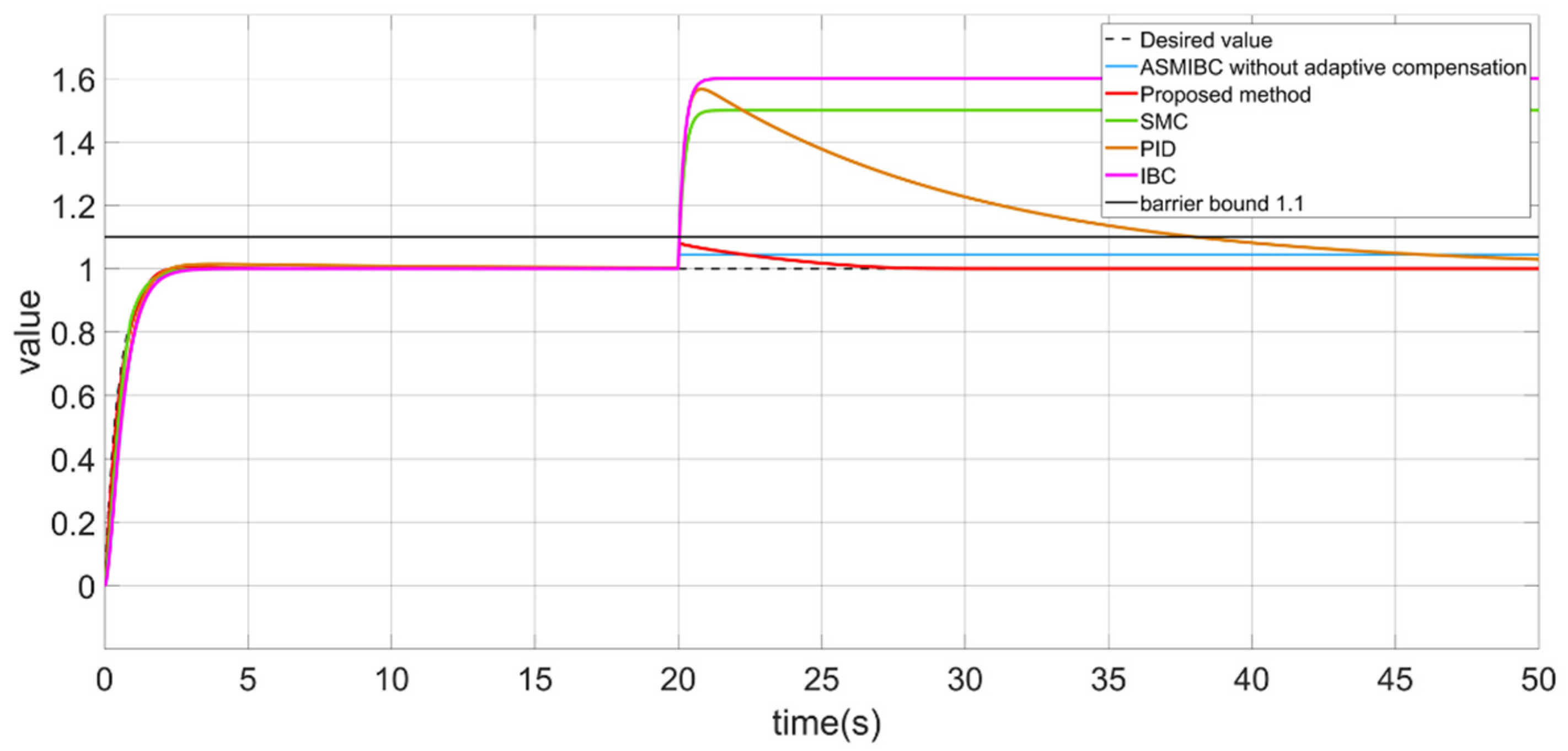
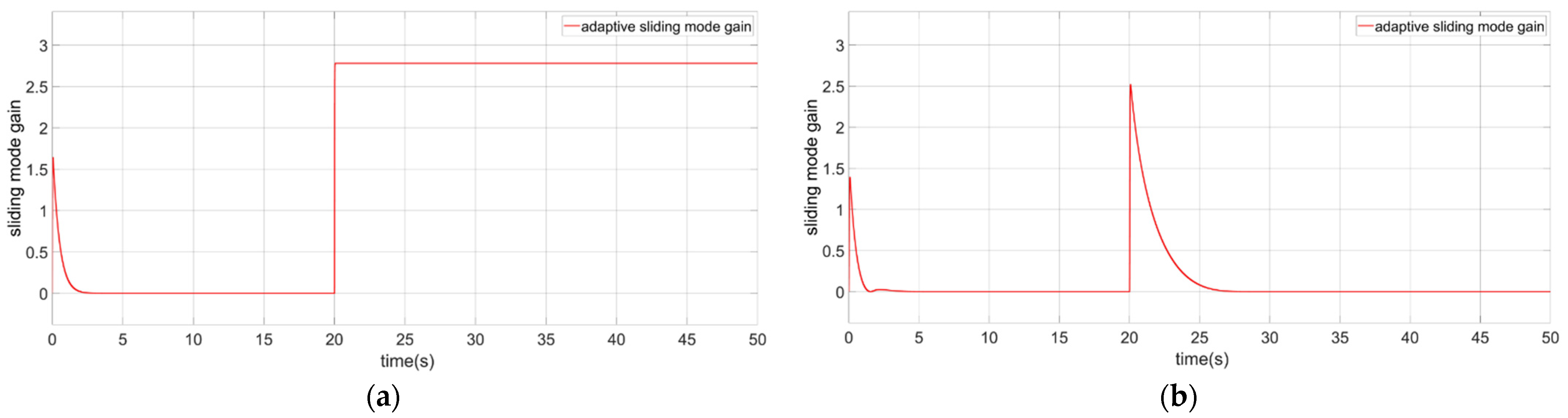
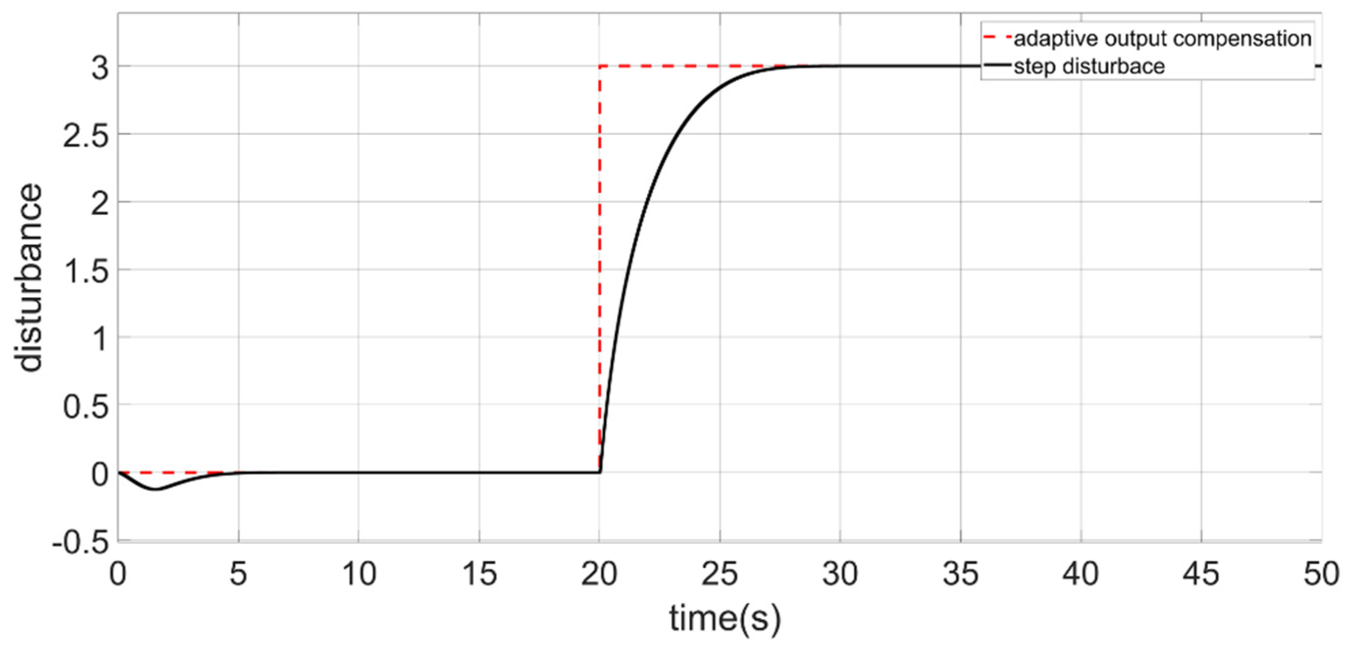
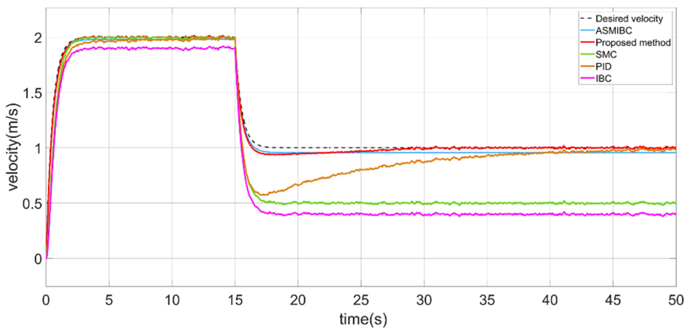
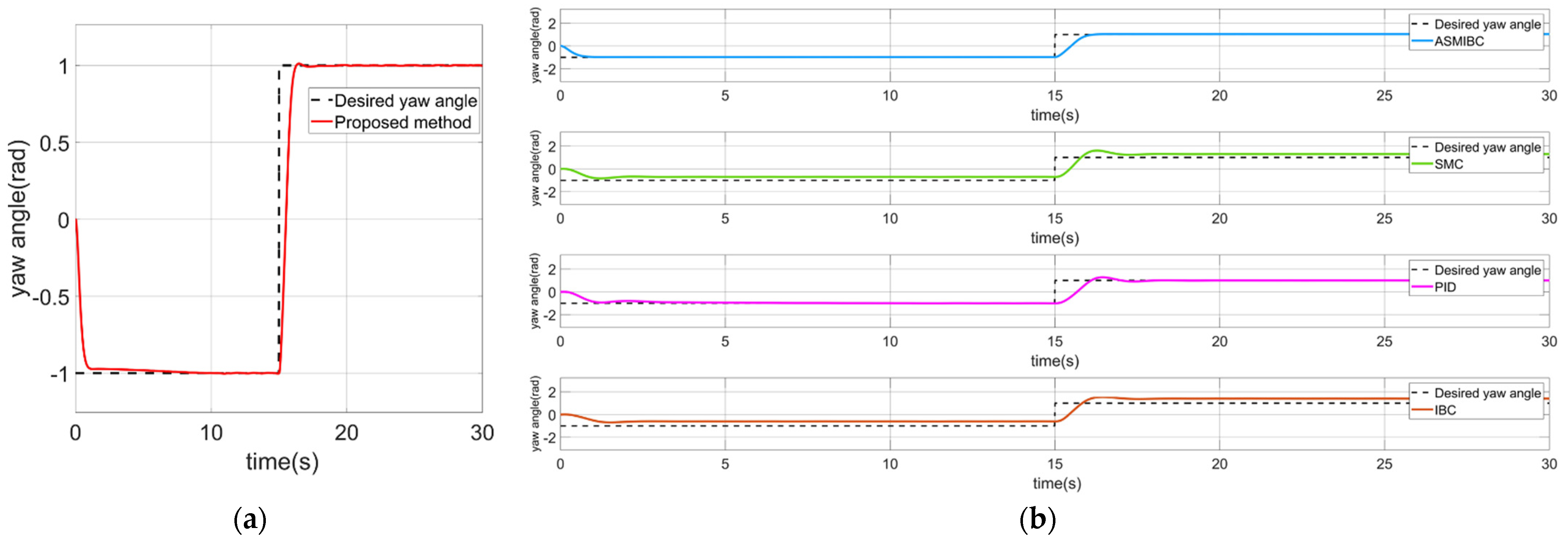
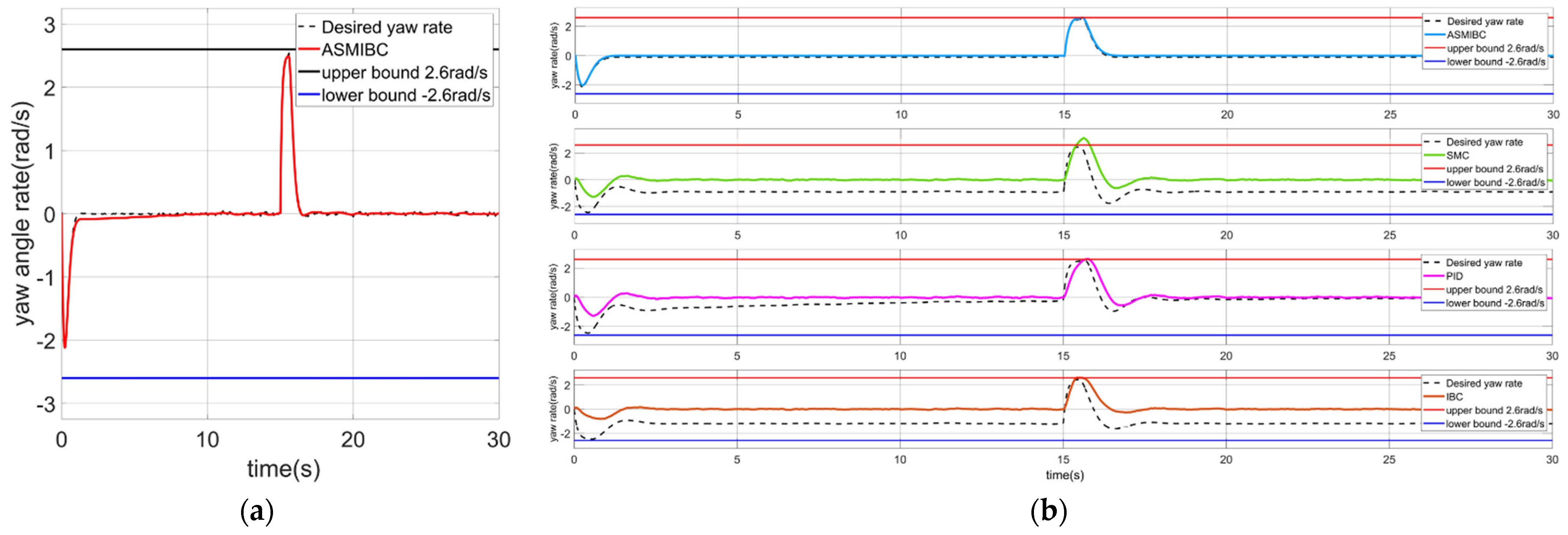
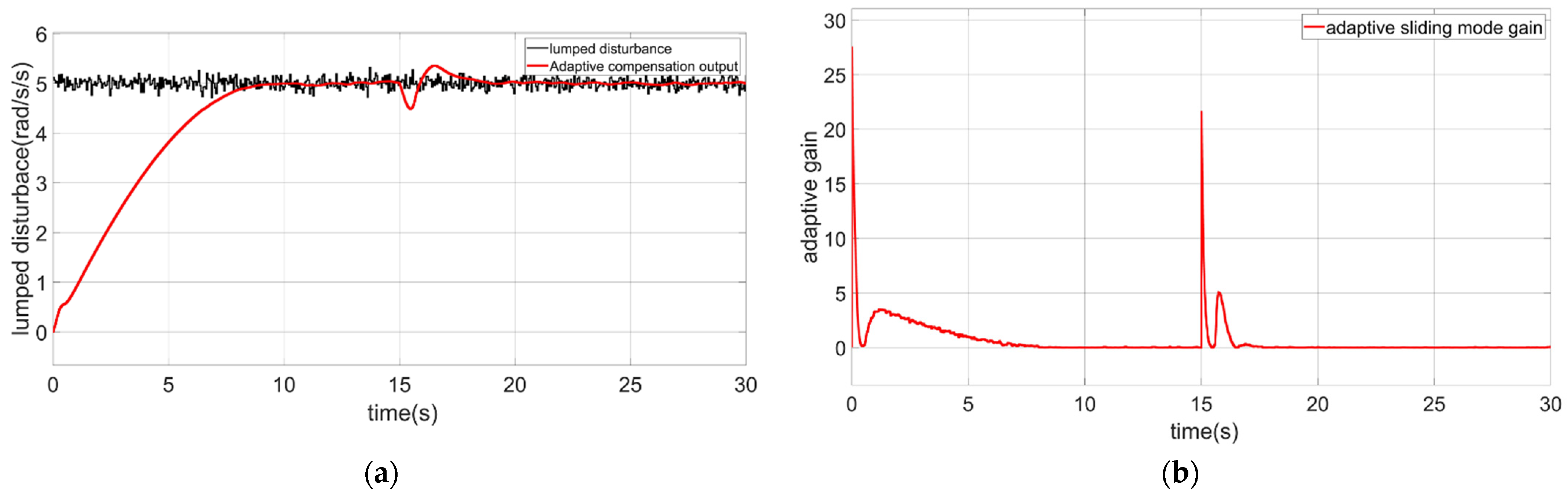
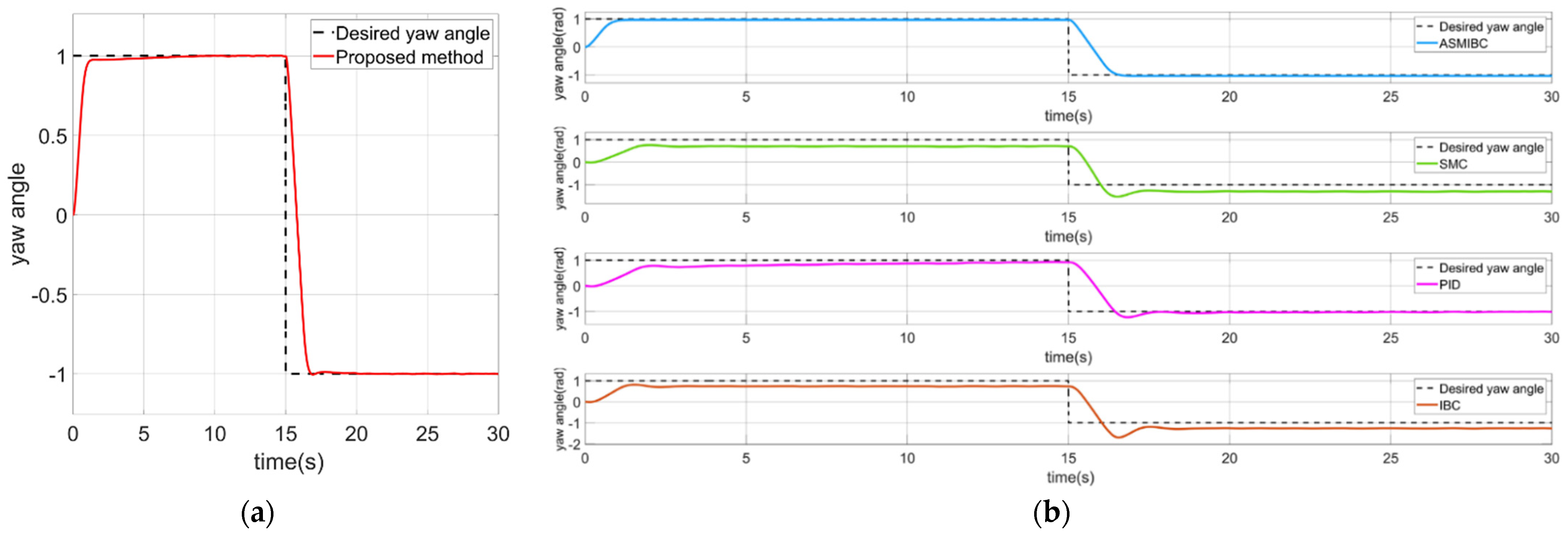
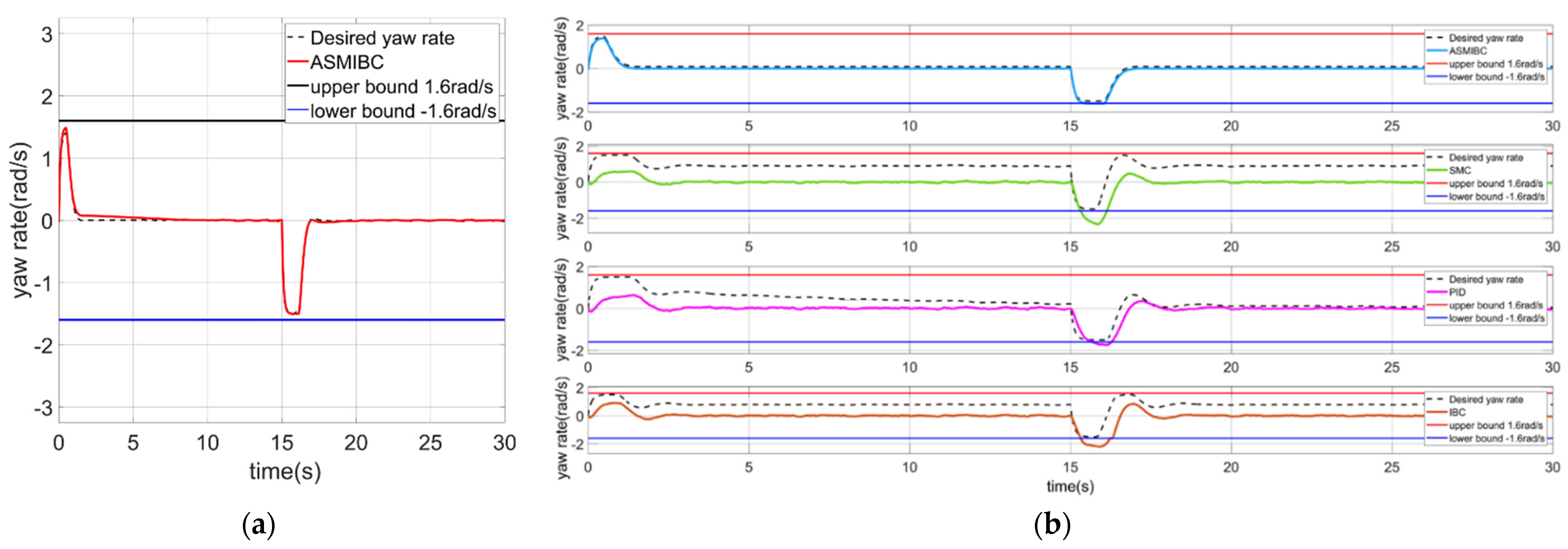
• ASMIBC is used to constrain the velocity and yaw angular velocity of the CDR in different environments. This control method solves the constraint failure of the traditional integral barrier control (IBC) when the desired state is a constant. The gain of the sliding mode is adaptively adjusted by the error between the limit state and the actual state, which improves the robustness of the controller. In addition, adaptive rate is designed for unknown and time-varying lumped disturbances. Compare simulation results with other control methods, like SMC, PID, and traditional IBC.

The paper is organized as follows: In Section 2, some preliminary work is presented and a brief introduction to the CDR is given. In Section 3, the dynamic model of CDR on the ground and water surface is introduced. The kinematic model is analyzed in the Frenet–Serret coordinate system. In Section 4, FLOS and ASMIBC are introduced, and a detailed proof of convergence is presented. Comparative analysis of the simulation results in the scenarios is discussed in Section 5.

2. Preliminaries Work and CDR Introduction

2.1. Preliminaries

In this section, three lemmas are introduced as the basis for the proof of the subsequent results. Lemma 1 is used to prove that the error of sideslip angle observer can converge in finite time. Lemma 2 is used to prove that the error of heading angle and error of velocity based on the ASMIBC algorithm can converge. Lemma 3 is used to prove that the proposed FLOS algorithm can guarantee the convergence of the robot’s position error. The three Lemmas are shown as follows:

Lemma 1. 

For a nonlinear system$\dot{x}=f(x,t)$, where$x(t)\in R^n$denotes the system state,$f$is continuous and smooth function in the domain of definition$U$. Suppose there exists a continuous and positive definite function$V(x)$satisfying [39]:

$$\mathsf{\Omega }\to R,\mathsf{\Omega }\subseteq U=R^n$$

$$\dot{V}(x)\le -\alpha V^P(x)+\vartheta ,x\in \mathsf{\Omega }\backslash \left\{0\right\}$$

where $\alpha >0$, $0<p<1$, $0<\vartheta <\infty$, the system state can converge to the vicinity of the equilibrium point in the limited time $T$, and $T\le V{(x_0)}^{1-p}/\left[\left(1-p\right)\left(\alpha -\epsilon \right)\right]$, the set of residuals satisfies $\underset{t\to T}{\lim }x\in \left(V^p(x)<\upsilon /\epsilon \right)$, where $\epsilon \in \left(0,a\right)$.

Lemma 2. 

The continuously positive differentiable integral barrier Lyapunov function (IBLF) is defined as [40]

$$V(e_i,\overline{H},i_d)={\displaystyle {\int }_0^{ei}\frac{\sigma {\overline{H}}^2}{{\overline{H}}^2-{\left(\sigma +i_d\right)}^2}}d\sigma$$

where $e_i=i-i_d$, $i_d$ is a continuously differentiable desired target satisfying $\left|i_d\right|\le \overline{H}$. $\overline{H}$ is a positive constant related to the system state barrier. In set ${\mathsf{\Omega }}_i$, $V_i$ always satisfies the following inequality:

$$\frac{e_i^2}{2}\le V_i\le \frac{{\overline{H}}^2{e}_i^2}{{\overline{H}}^2-i^2}$$

Lemma 3. 

For a nonlinear system$\dot{x}=f(x,t)$, where$x(t)\in R^n$denotes the system state,$f$is continuous and smooth function in the domain of definition$U$,$U\to R$. Suppose there exists a continuous and positive definite function$V(x)$satisfying [41]:

$$\dot{V}(x)\le -\alpha V^P(x)-\beta V^P(x),x\in U\backslash \left\{0\right\}$$

where $\alpha >0$, $\beta >0$, $0<p<1$ are positive constants, then the system is stable for a limited time $T$. Convergence time $T$ satisfies: $T\le \frac{1}{\alpha (1-p)}\ln \frac{\alpha V{(x_0)}^{1-p}+\beta }{\beta }$.

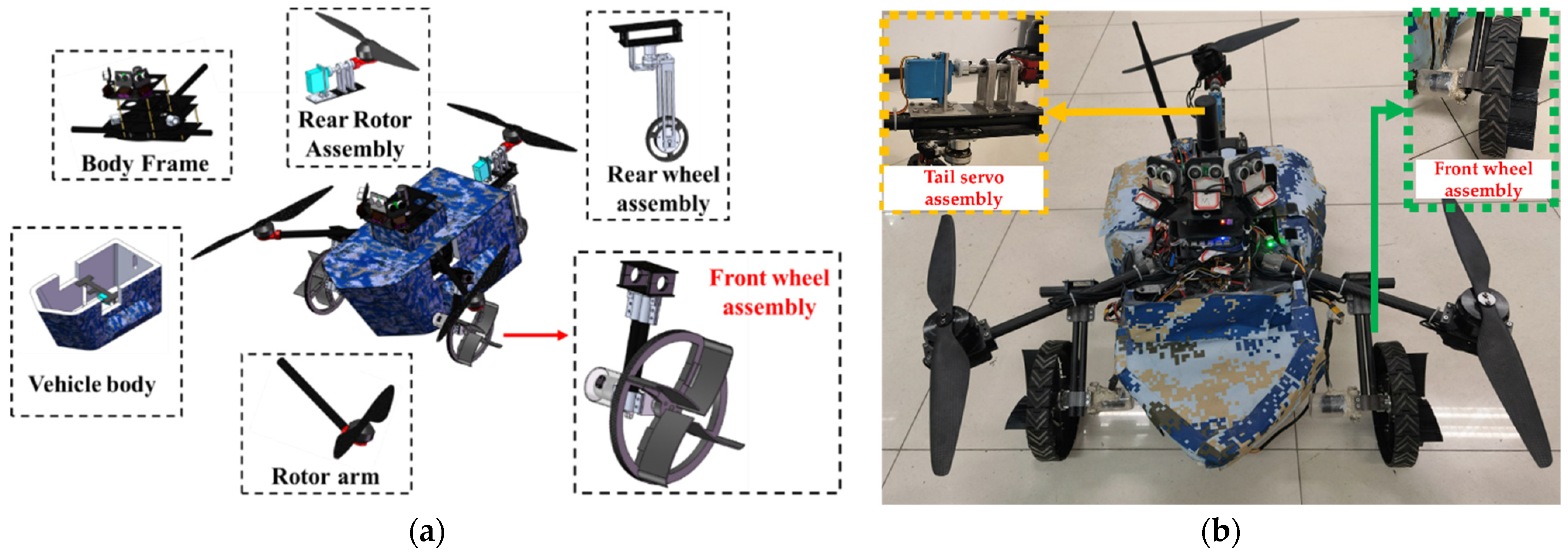
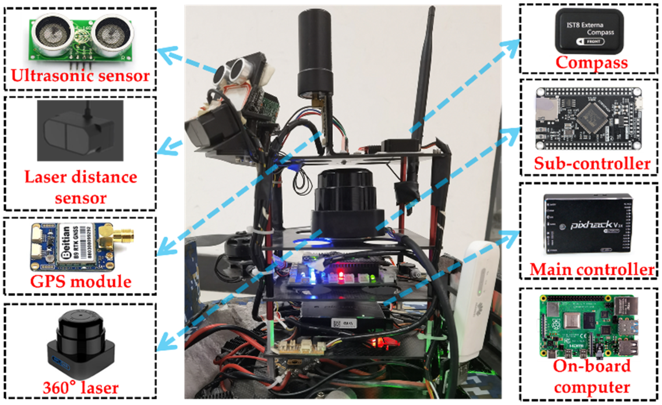
2.2. Cross-Domain Robot

The CDR designed by us can work on the ground, water surface, and in the air, but the aerial control of the CDR is not the key point in this paper. We mainly study the robot control on the ground and the water surface.

To reduce the mass of the robot, an integrated wheel-paddle design is adopted. The CDR uses the same drive motor on the ground and the water surface. In the air, the CDR adopts tri-copter mechanical structure. The structure of the CDR is as shown in Figure 1.

In Figure 1b, the main actuators of the robot are introduced. The CDR uses three T-Motor U7 motors in the air. These motors are matched with three T-MOTOR FLAME 60 AHV electronic speed controller. Each motor adopts 16-inch blade. The three aerial drive units can provide a maximum lift of 12 kg for the robot. Two DJI RobotMaster M2006 motors are used on the ground. These motors are equipped with RobotMaster C610 electric speed controller. The tail servo of CDR adopts KST waterproof servo, which has a maximum output torque of 19 kg·cm. The robot uses the same driving unit when moving on the water surface and on the ground, so we have designed a waterproof shell for M2006 motor. The main sensors and controllers of the CDR are shown in Figure 2.

In Figure 2, the main sensors and controllers are introduced. To realize the ability of the robot to avoid obstacles autonomously, we use three HY-SR05 ultrasonic sensors and RPLIDAR-S1 laser to get the local obstacles information around the robot. BT-F9PK4 is used for the GPS module to provide global localization messages for the robot. Three TFminiPlus laser ranging sensors is used to get the negative obstacle, to prevent the robot from falling into the trap. IST8 of CUAV is used as the compass. STM32F4 is the main control chip on the sub controller to collect the messages of sensors and send them to the main controller. The main controller is Pixhack-V3x of CUAV, which integrates inertial measuring unit and barometer to obtain the attitude and height of the robot. On-board computer uses Raspberry pi 4B+ to plan the desired trajectory of the robot to avoid obstacles. The on-board computer is hidden in the cabin of the robot.

The main parameters of the CDR are shown in

Table 1. The main parameters of the CDR.

Parameter	Unit	Value
Mass	kg	6.5
Max length	cm	85
Max width	cm	55
Height	cm	75
Max buoyancy	kg	7.3
Wheel radius	cm	8
Length of the axle	cm	50
Rotational inertia of Z-axis	kg·m2	0.108

.

Autonomous trajectory tracking of the CDR on the water surface and the ground are shown in Figure 3.

3. Mathematic Model of CDR on the Ground and Water Surface

A CDR is a nonholonomic constrained underactuated structure on the ground and water surface. Therefore, this kind of robot is incapable of moving laterally. In the dynamic model, uncertainties from air resistance and mechanical friction losses disturb the robot as it moves on the ground. However, when the robot moves on the water surface, in addition to air resistance and mechanical friction losses, water resistance and wind interference should also be considered.

Before discussing the mathematical model, the following assumptions are made:

Assumption 1. 

The robot is a rigid body, whose mass distribution is homogeneous, and the shape structure is a port/starboard symmetric.

Assumption 2. 

The center of gravity of the robot’s body coincides with the geometric center.

Assumption 3. 

The heave, pitch, and roll motions on the horizontal plane are neglected.

Assumption 4. 

The non-diagonal terms of inertial and drag matrices are small compared to the main diagonal terms, and can be neglected.

Assumption 5. 

The drive force generated by the motors meets the performance requirements of the robot.

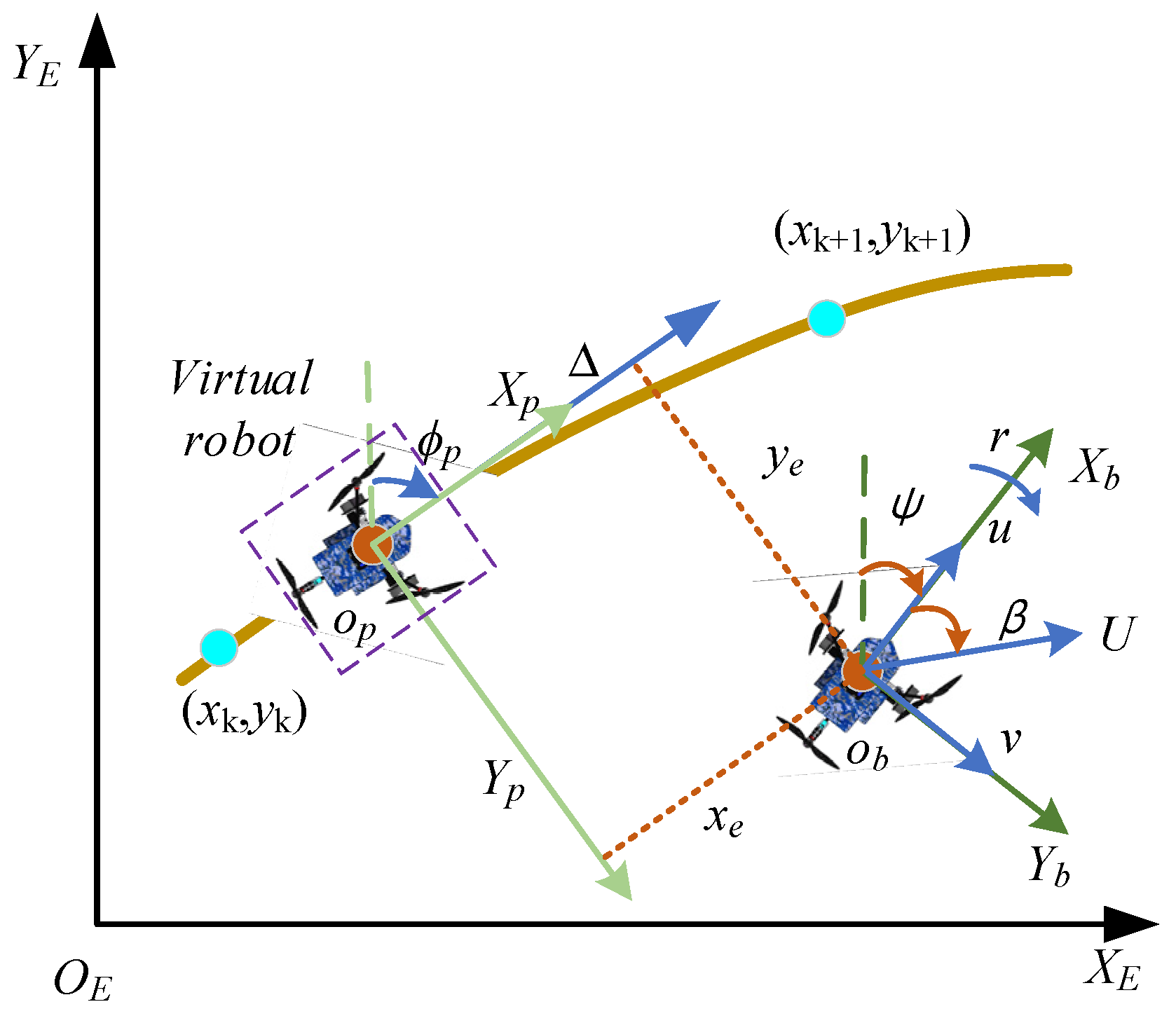
3.1. CDR Kinematic Model in Frenet-Secret Frame

In [15,17], the kinematic model in the body frame can be expressed as:

$$\dot{q}=R\eta$$

(1)

In Formula (1), $q=\left[x,y,\psi \right]$ is the position and orientation of the robot in earth coordinates, and $\eta =\left[u,v,r\right]$ is the longitudinal velocity, lateral velocity, and yaw angular velocity of the CDR. R matrix is the transformation matrix of the robot from the body frame to the earth frame, where R is

$$R=\left[\begin{array}{ccc}\cos \psi & -\sin \psi & 0\\ \sin \psi & \cos \psi & 0\\ 0& 0& 1\end{array}\right]$$

The robot in Frenet–Serret coordinate system is as shown in Figure 4.

In Figure 4, $E$ is the inertial coordinate frame. $P$ presents the Frenet–Serret coordinate frame. $b$ is the body coordinate frame. ${\varphi }_p$ is the angle between $X_p$ axis and $Y_E$ axis. $\Delta$ is the forward-looking distance. $\psi$ is the yaw angle of the robot. $r$ is the yaw angular velocity. $\beta$ is the side-slip angle. $u$ is the longitudinal velocity. $v$ is the lateral velocity. $U$ is the actual linear velocity of the robot motion. $x_e$ and $y_e$ are errors between current position of the robot and the desired position converted into $P$ coordinate.

According to [34], the mathematical model of position error in the Frenet–Serret coordinate frame can be expressed as:

$$\left[\begin{array}{l}{x}_e\\ y_e\end{array}\right]=\left[\begin{array}{cc}\cos {\varphi }_p& \sin {\varphi }_p\\ -\sin {\varphi }_p& \cos {\varphi }_p\end{array}\right]\left[\begin{array}{l}x-x_k(\omega )\\ y-y_k(\omega )\end{array}\right]$$

(2)

$x_k(\omega )$ and $y_k(\omega )$ are the parametrized desired trajectory. Formula (2) takes the derivative of time t and substitutes it into Formula (1) to obtain

$${\dot{x}}_e=u\cos (\psi -{\varphi }_p)-v\sin (\psi -{\varphi }_p)+{\dot{\varphi }}_p{y}_e-\dot{\omega }\sqrt{x^{\text{'}}{}_k^2(\omega )+y^{\text{'}}{}_k^2(\omega )}\cos (\varphi +\alpha )$$

(3)

because $\alpha =\mathrm{atan}2(-y^{\text{'}}{}_k^2(\omega ),x^{\text{'}}{}_k^2(\omega ))=-\varphi$, Formula (3) can be expressed as:

$${\dot{x}}_e=u\cos (\psi -\varphi )-v\sin (\psi -\varphi )+\dot{\varphi }{y}_e-u_p$$

(4)

$u_p=\dot{\omega }\sqrt{x^{\text{'}}{}_k^2(\omega )+y^{\text{'}}{}_k^2(\omega )}$ is a virtual variable which is designed to stabilize the $x_e$.

$$y_e=u\sin (\psi -{\varphi }_p)+v\cos (\psi -{\varphi }_p)-\dot{\varphi }{x}_e$$

(5)

$\beta =\arctan (v/u)$ can be considered as the angle of robot deflection caused by lateral velocity due to cross-winds and currents on the water surface and skidding on the ground.

The position error derivative can be expressed as:

$$\{\begin{array}{l}{\dot{x}}_e=u\cos (\psi -\varphi )-u\sin (\psi -\varphi )\tan \beta +\dot{\varphi }{y}_e-u_p\\ {\dot{y}}_e=u\sin (\psi -\varphi )+u\cos (\psi -\varphi )\tan \beta -\dot{\varphi }{x}_e\end{array}$$

(6)

Remark 1. 

In [35,36], assume $\beta \le 5^{\circ }$, so $\sin \beta \approx \beta$, $\cos \beta \approx 1$. However, this assumption is conservative and does not conform to the actual situation, especially for small USVs and multi-habitat robots, which are more likely to be disturbed by the environment.

3.2. Dynamic Model of CDR on the Ground and the Water Surface

The lateral velocity constraint is considered in the WMR model. However, to unify the mathematical model of the robot on the ground and the water surface, the lateral velocity constraint is no longer considered. According to ref. [17], the Lagrange dynamic equation for the CDR on the ground is

$$M(q)\ddot{q}+C_m(q,\dot{q})q+F(\dot{q})+{\tau }_d=B(q)\tau$$

(7)

where $M$ is the symmetric and positive definite inertia matrix, $C_m$ is the centripetal and Coriolis matrix, $F(\dot{q})$ is the drag force, $B_{\left(q\right)}$ is the input transformation matrix, and $\tau$ is the torque generated by the robot drive motor, and ${\tau }_d$ is the unknown disturbance. These matrices can be expressed as

$$M(q)=\left[\begin{array}{ccc}m& 0& md\sin \psi \\ 0& m& -md\cos \psi \\ md\sin \psi & -md\cos \psi & I\end{array}\right], B(q)=\frac{1}{r}\left[\begin{array}{cc}\cos \psi & \cos \psi \\ \sin \psi & \sin \psi \\ L& -L\end{array}\right], \tau =\left[\begin{array}{l}{\tau }_l\\ {\tau }_r\end{array}\right]$$

$C_m(q,\dot{q})={\left[\begin{array}{ccc}md{\dot{\psi }}^2\cos \psi & md{\dot{\psi }}^2\sin \psi & 0\end{array}\right]}^T$, where $m$ is the mass of the robot and $I$ is the rotational inertia, and L is the length of the axle. $\psi$ is the yaw angle. $r$ is the radius of the wheel. $d$ is the distance from the center of gravity of the robot to the geometric center of the robot. ${\tau }_l$ and ${\tau }_r$ are the torques output by the left and right motors. According to Assumption 2, $C_m=0$, and $M$ matrix can be rewritten as $M\left(q\right)=\left[\begin{array}{ccc}m& 0& 0\\ 0& m& 0\\ 0& 0& I\end{array}\right]$.

Take the time derivative of Formula (1), substitute it into Formula (7) and left multiply $R^{-1}$, which yields:

$$\overline{C}\eta +\overline{M}\dot{\eta }+\overline{F}(\dot{q})+{\overline{\tau }}_d=\overline{B}\tau$$

(8)

where $\overline{C}=R^{-1}M\dot{R}$, $\overline{M}=R^{-1}MR$, $\overline{B}=R^{-1}B$. $\overline{F}(\dot{q})={\left[\begin{array}{ccc}{f}_u& f_v& f_r\end{array}\right]}^T$, ${\overline{\tau }}_d={\left[\begin{array}{ccc}{d}_u& d_v& d_r\end{array}\right]}^T$.

Formula (8) can be expressed in algebraic form as:

$$\{\begin{array}{l}\dot{u}=\left(F_u-f_u-d_u\right)/m+vr\\ \dot{v}=-ur-\left(f_v+d_v\right)/m\\ \dot{r}=\left(T_r-f_r-d_r\right)/I\end{array}$$

(9)

where $F_u=({\tau }_l+{\tau }_r)/\mathrm{r}$, $T_r=({\tau }_l-{\tau }_r)\ast L/\mathrm{r}$.

According to ref. [15], the dynamics of the robot on the water surface can be modeled as:

$$M\dot{\eta }+C\left(\eta \right)+D\left(\eta \right)\eta =F(t)+d\left(\eta ,t\right)$$

(10)

$F={\left[\begin{array}{ccc}{F}_u& 0& T_r\end{array}\right]}^T$ is the control input. The unknown lumped disturbances includes unmodeled dynamic disturbances, uncertainties and external disturbances can be expressed as: $d={\left[\begin{array}{ccc}{d}_u& d_v& d_r\end{array}\right]}^T$,

$$M=\left[\begin{array}{ccc}{m}_{11}& 0& 0\\ 0& m_{22}& m_{23}\\ 0& m_{32}& m_{33}\end{array}\right], C\left(\eta \right)=\left[\begin{array}{ccc}0& 0& C_{13}\left(\eta \right)\\ 0& 0& C_{23}\left(\eta \right)\\ -C_{13}\left(\eta \right)& -C_{23}\left(\eta \right)& 0\end{array}\right], D=\left[\begin{array}{ccc}{d}_{11}& 0& 0\\ 0& d_{22}& d_{23}\\ 0& d_{32}& d_{33}\end{array}\right]$$

According to Assumption 4, the non-diagonal parameters of internal matrix $M$ are small enough to be neglected. This approach is also used in [15,41].

The CDR dynamic model on the water surface can be expressed as:

$$\{\begin{array}{l}\dot{u}=\frac{m_{22}}{m_{11}}\upsilon \omega -\frac{X_u}{m_{11}}u-\frac{X_{\left|u\right|u}}{m_{11}}\left|u\right|u+\frac{F_u}{m_{11}}+\frac{d_u}{m_{11}}\\ \dot{\upsilon }=-\frac{m_{11}}{m_{22}}u\omega -\frac{Y_u}{m_{22}}\upsilon -\frac{Y_{\left|v\right|v}}{m_{22}}\left|\upsilon \right|\upsilon +\frac{d_v}{m_{11}}\\ \dot{\omega }=\frac{m_{11}-m_{22}}{m_{33}}u\upsilon -\frac{N_{\omega }}{m_{33}}\omega -\frac{N_{\left|\omega \right|\omega }}{m_{33}}\left|\omega \right|\omega +\frac{T_r}{m_{33}}+\frac{d_r}{m_{33}}\end{array}$$

(11)

$m_{11}=m-X_{\dot{u}}$, $m_{22}=m-Y_{\dot{v}}$, $m_{33}=I_z-N_{\dot{r}}$ are inertia mass parameters. $X_{\dot{u}}$$Y_{\dot{v}}$$N_{\dot{r}}$ is extended inertia mass parameters. $I_z$ is the rotational inertia of the robot rotates around the Z-axis. $X_u$, $X_{\left|u\right|u}$, $Y_u$, $Y_{\left|v\right|v}$, $N_{\omega }$, $N_{\left|\omega \right|\omega }$ are hydrodynamic damping parameters.

According to Assumption 5, we do not discuss the conversion of motor torque to traction and rotation torque. The traction force and rotation torque of the CDR in both water and ground environments are expressed as $F_u$ and $T_r$.

By comparing Formula (9) with Formula (11), the dynamic models of the robot on the ground and the water surface are similar except for the changes of robot inertia parameters and the drag force caused by different working environments. The dynamics equations of the CDR can be expressed uniformly as:

$$\{\begin{array}{l}\dot{u}=k_1\upsilon \omega +f_u+\frac{F_u}{m_1}+\frac{d_u}{m_1}\\ \dot{\upsilon }=-k_{2}u\omega +f_{\upsilon }+\frac{d_{\upsilon }}{m_2}\\ \dot{\omega }=k_{3}u\upsilon +f_r+\frac{T_r}{m_3}+\frac{d_r}{m_3}\end{array}$$

(12)

When the robot moves on the water surface, dynamic parameters of the CDR can be expressed as: $m_1=m-X_{\dot{u}}$, $m_2=m-Y_{\dot{v}}$, $m_3=I-N_{\dot{r}}$, $k_1=m_{22}/m_{11}$, $k_2=m_{11}/m_{22}$, $k_3=(m_{11}-m_{22})/m_{33}$, $f_u=-\frac{X_u}{m_{11}}u-\frac{X_{\left|u\right|u}}{m_{11}}\left|u\right|u$, $f_{\upsilon }=-\frac{Y_u}{m_{22}}\upsilon -\frac{Y_{\left|v\right|v}}{m_{22}}\left|\upsilon \right|\upsilon$, $f_{\omega }=-\frac{N_{\omega }}{m_{33}}\omega -\frac{N_{\left|\omega \right|\omega }}{m_{33}}\left|\omega \right|\omega$. $f_u$, $f_{\upsilon }$, $f_{\omega }$ are water force.

When the robot moves on the ground, the dynamic parameters are $m_1=m$, $m_2=m$, $m_3=I$, $k_1=1$, $k_2=1$, $k_3=1$. $f_u=0$, $f_v=0$, $f_r=0$. $f_i(i=u,v,r)$ are the air force of the environment. $d_i(i=u,v,r)$ are unknown and time-varying disturbances.

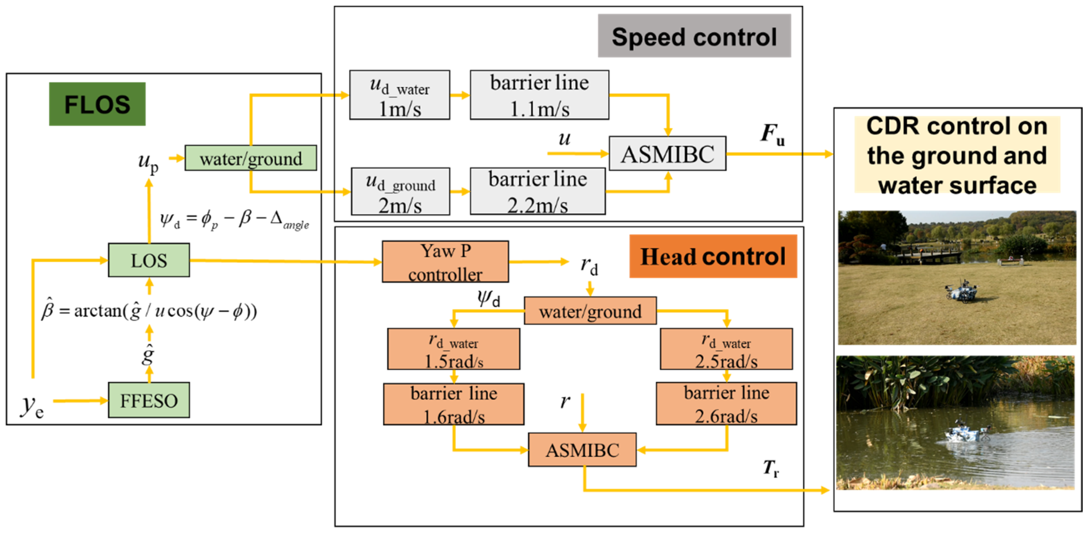
4. FLOS Algorithm and ASMIBC

To solve the control problem mentioned above, a FLOS navigation algorithm is adopted to reduce trajectory tracking errors caused by the lateral velocity. The ASMIBC constrains the linear velocity and yaw angular velocity.

The control structure of the CDR on the ground and the water surface is shown in Figure 5.

4.1. FLOS with FESO

Considering the term containing the uncertain side-slip angle $\beta$ in Formula (6) as an uncertain state, we define new state $g$ as $g=u\cos (\psi -\varphi )\tan \beta$. Therefore, side-slip angle $\beta =\arctan (g/u\cos (\psi -\varphi ))$.

To observe the side-slip angle $\beta$ in finite time, a finite-time converge observer is designed as

$$\{\begin{array}{l}{\dot{\widehat{y}}}_e=\widehat{g}+u\sin (\psi -{\varphi }_p)-{\dot{\varphi }}_p{x}_e-l_1{f}_1({\tilde{y}}_e)\\ \dot{\widehat{g}}=-l_2{f}_2({\tilde{y}}_e)\end{array}$$

(13)

where ${\widehat{y}}_e$ is the observation of $y_e$, ${\tilde{y}}_e={\widehat{y}}_e-y_e$. $\widehat{g}$ is the observation of $g$. $l_1$, $l_2$ are positive adjustable parameters, $f_1({\tilde{y}}_e)$, $f_2({\tilde{y}}_e)$ can be expressed as

$$\{\begin{array}{l}{f}_1({\tilde{y}}_e)=k_1{\left|{\tilde{y}}_e\right|}^{\frac{1}{2}}sign({\tilde{y}}_e)+{\tilde{y}}_e\\ f_2({\tilde{y}}_e)=\frac{3k_1}{2}{\left|{\tilde{y}}_e\right|}^{\frac{1}{2}}sign({\tilde{y}}_e)+\frac{k_1^2}{2}sign({\tilde{y}}_e)+{\tilde{y}}_e\end{array}$$

(14)

Take ${\tilde{y}}_e$ derivation for time t and substitute it into the second line of Formulas (6) and (13), which yields

$$\{\begin{array}{l}{\dot{\tilde{y}}}_e=\widehat{g}+u\sin (\psi -\varphi )-\dot{\varphi }{x}_e-l_1{f}_1({\tilde{y}}_e)-u\sin (\psi -\varphi )-\dot{\varphi }{x}_e-g\\ \begin{array}{cc}& =\tilde{g}-l_1{f}_1({\tilde{y}}_e)\end{array}\\ \dot{\tilde{g}}=-l_2{f}_2({\tilde{y}}_e)-\dot{g}\\ {\dot{f}}_1({\tilde{y}}_e)=\left(\frac{1}{2}{\tilde{y}}_e^{-1/2}sign({\tilde{y}}_e)+1\right)\left(\tilde{g}-l_1{f}_1({\tilde{y}}_e)\right)\end{array}$$

(15)

Remark 2. 

$\beta$is slowly time-varying, so$\dot{\beta }\approx 0$,$\dot{g}\approx u\sin (\psi -\varphi )(\dot{\psi }-\dot{\varphi })\tan \beta$. $u$,$\dot{\psi }$,$\dot{\varphi }$are bounded, so$\left|\dot{g}\right|\le h_{\max }$. $h_{\max }$is a positive constant.

Theorem 1. 

The observer satisfies Formula (13), the observation error can converge in finite time T, where$T\le V{\left({\tilde{y}}_e(0)\right)}^{1/2}/\left[\frac{1}{2}(\frac{k_1}{2k_{\min }}-{\sigma }_1)\right]$, to the neighborhood of the equilibrium point$(0,0)$, where${\sigma }_1$is a constant and${\sigma }_1\in \left(0,\frac{k_1}{2k_{\min }}\right)$.

The proof of Theorem 1 can be found in Appendix A.

In contrast to the idealized assumptions for the uncertainty term $g$ in [38], we adopt a simpler and clearer approach to prove the convergence of the observer.

The FLOS is designed as:

$${\psi }_d={\varphi }_p-\arctan \left(\tan \widehat{\beta }+\frac{y_e+k_y{\left|y_e\right|}^{p}sign(y_e)}{\Delta }\right)$$

(16)

$\Delta$ is the forward-looking distance. where $0<p<1$, $k_y$ is the positive adjustable parameter. The speed $u_p$ is designed to make the convergence of the position error $x_e$, the virtual variable $u_p$ is

$$u_p=k_1{x}_e+k_2{\left|x_e\right|}^{p}sign(x_e)+u\cos (\psi -{\varphi }_p)+u\sin (\psi -{\varphi }_p)\tan \widehat{\beta }$$

(17)

where $0<p<1$, yaw angle satisfies $\psi \approx {\psi }_d$ by control, so $\psi -{\varphi }_p={\psi }_d-{\varphi }_p$. Therefore,

$$\sin \left({\psi }_d-{\varphi }_p\right)=-\frac{y_e+k_y{\left|y_e\right|}^{p}sign(y_e)+\Delta \tan \widehat{\beta }}{\sqrt{{\Delta }_2+{\left(y_e+k_y{\left|y_e\right|}^{p}sign(y_e)+\Delta \tan \widehat{\beta }\right)}^2}}$$

(18)

$$\cos \left({\psi }_d-{\varphi }_p\right)=-\frac{\Delta }{\sqrt{{\Delta }_2+{\left(y_e+k_y{\left|y_e\right|}^{p}sign(y_e)+\Delta \tan \widehat{\beta }\right)}^2}}$$

(19)

Substituting Formulas (17)–(19) into (6) yields

$${\dot{x}}_e=-k_1{x}_e-k_2{\left|x_e\right|}^{p}sign(x_e)-u\sin (\psi -{\varphi }_p)(\tan \beta -\tan \widehat{\beta })+{\dot{\varphi }}_p{y}_e$$

(20)

$$\begin{array}{l}{\dot{y}}_e=-\frac{u(y_e+k_y{\left|y_e\right|}^{p}sign(y_e))}{\sqrt{{\Delta }_2+{\left(y_e+k_y{\left|y_e\right|}^{p}sign(y_e)+\Delta \tan \widehat{\beta }\right)}^2}}\\ +\frac{u(\tan \widehat{\beta }-\tan \beta )}{\sqrt{{\Delta }_2+{\left(y_e+k_y{\left|y_e\right|}^{p}sign(y_e)+\Delta \tan \widehat{\beta }\right)}^2}}-{\dot{\varphi }}_p{x}_e\end{array}$$

(21)

According to Theorem 1, we have proved that $\widehat{\beta }\approx \beta$ in finite time. Thus,

$${\dot{x}}_e=-k_1{x}_e-k_2{\left|x_e\right|}^{p}sign(x_e)+{\dot{\varphi }}_p{y}_e$$

(22)

$${\dot{y}}_e=-\frac{u(y_e+k_y\left|y_e\right|sign(y_e))}{\sqrt{{\Delta }_2+{\left(y_e+k_y{\left|y_e\right|}^{p}sign(y_e)+\Delta \tan \widehat{\beta }\right)}^2}}-{\dot{\varphi }}_p{x}_e$$

(23)

The convergence proof of position errors x_e and y_e can be found in Appendix B.

4.2. ASMIBC for Yaw Angle and Linear Velocity of the CDR

According to the dynamic mathematical model, the drag forces are different when the CDR moves on the water surface and the ground. The system parameters change in different environments too. Interferences caused by environmental disturbances and parameter uncertainties are considered as unknown and time-varying lumped disturbances. The yaw angle and linear velocity control system can be regarded as second-order nonlinear single input single output system with uncertain disturbances, which is shown as follows:

$$\{\begin{array}{l}{\dot{x}}_1=x_2\\ {\dot{x}}_2=f(x)+g(x)u+\eta (x)\\ y_1=x_1\end{array}$$

(24)

where $x={\left[\begin{array}{cc}{x}_1& x_2\end{array}\right]}^T$, $x_1$, and $x_2$ are system states.$g(x)$, and $f(x)$ are smooth functions. $\eta (x)$ is the unknown lump disturbance. $u$ is control input, $y_1$ is control output. $f(x)$ is the certain term of system. $y_d$ is the desired state of $x_1$. $x_1$, $x_2$, $y_d$, and ${\dot{y}}_d$ are continuous and derivable.

Define $z_1=x_1-y_d$, $z_2=x_2-{\alpha }_1$, ${\alpha }_1$ is the virtual state. $\left|z_2\right|<k_h$, $k_h$ is the maximum of state error, $\xi =z_2/k_h<1$. Define Lyapunov function $V_0=\frac{1}{2}{z}_1^2$. $V_0$ takes the derivative of time t yields

$${\dot{V}}_0=z_1^{}\left({\dot{x}}_1-{\dot{y}}_d\right)=z_1^{}\left(z_2+{\alpha }_1-{\dot{y}}_d\right)$$

(25)

${\alpha }_1=-k_0{z}_1+{\dot{y}}_d$, $k_0$ is a positive constant.

Define Lyapunov function $V_1\left(z_2,{\alpha }_1\right)$ as

$$V_1\left(z_2,{\dot{\alpha }}_1\right)=V_0+{\displaystyle {\int }_0^{z_2}\frac{\sigma {\overline{x}}_2^2}{{\overline{x}}_2^2-{\left(\sigma +{\alpha }_1\right)}^2}d\sigma }$$

(26)

$\left|x_2\right|<{\overline{x}}_2$, ${\overline{x}}_2$ is the upper limit of the state $x_2$. $V_1$ takes the derivative of time t yields

$$\begin{array}{l}{\dot{V}}_1=\frac{\partial V_1}{\partial z_2}{\dot{z}}_2+\frac{\partial V_1}{\partial {\dot{y}}_d}{\dot{\alpha }}_1+z_1{z}_2\\ \begin{array}{cc}& =\end{array}\frac{z_2{\overline{x}}_2^2}{{\overline{x}}_2^2-x_2^2}{\dot{z}}_2+z_2\left(\frac{{\overline{x}}_2^2}{{\overline{x}}_2^2-x_2^2}-l_1\right){\dot{\alpha }}_1+z_1{z}_2\\ \begin{array}{cc}& =\end{array}\frac{z_2{\overline{x}}_2^2}{{\overline{x}}_2^2-x_2^2}\left(f(x)+g(x)u+\eta (x)-{\dot{\alpha }}_1\right)-\frac{z_2{\overline{x}}_2^2}{{\overline{x}}_2^2-x_2^2}{\dot{\alpha }}_1-z_2{l}_1{\dot{\alpha }}_1+z_1{z}_2\end{array}$$

(27)

where $l_1=\frac{{\overline{x}}_2^2}{2z_2}\ln \frac{\left({\overline{x}}_2^2+x_2^2\right)\left({\overline{x}}_2^2-{\alpha }_1^2\right)}{\left({\overline{x}}_2^2-x_2^2\right)\left({\overline{x}}_2^2+{\alpha }_1^2\right)}$, the traditional IBC controller is designed as

$$u=\frac{1}{g(x)}\left(-k_1{z}_2-f(x)-\eta (x)+2{\dot{\alpha }}_1-\frac{{\overline{x}}_2^2-x_2^2}{{\overline{x}}_2^2}{z}_1\right)+\frac{{\overline{x}}_2^2-x_2^2}{{\overline{x}}_2^2}{l}_1{\dot{\alpha }}_1$$

(28)

when $x_2^{}\to {\overline{x}}_2^{}$, $l_1\to \infty$, thus the control output $u$ is adjusted to constrain the state of the system. However, when ${\alpha }_1$ is constant, the controller degenerates into a traditional proportional controller based on backstepping method. For example, when the desired trajectory of a robot is a straight line moving at a constant speed, IBC loses the ability to constrain the speed.

Based on the idea of SMC and integral barrier control (IBC), the control output is defined as $u=u_1+u_2$. For the uncertain lumped disturbance $\eta (x)$ an adaptive law is designed. $\widehat{\eta }(x)$ is the estimation of $\eta (x)$, and $\tilde{\eta }(x)=\widehat{\eta }(x)-\eta (x)$, $\eta (x)$ is a constant, so $\dot{\tilde{\eta }}(x)=\dot{\widehat{\eta }}(x)$.

$$u_1=\frac{1}{g(x)}\left(-k_1{z}_2-f(x)-\widehat{\eta }(x)+2{\dot{\alpha }}_1-\frac{{\overline{x}}_2^2-x_2^2}{{\overline{x}}_2^2}{z}_1\right)+\frac{{\overline{x}}_2^2-x_2^2}{{\overline{x}}_2^2}{l}_1{\dot{\alpha }}_1, u_2=-\frac{1}{g(x)}{k}_{2}sign(z_2)$$

Define Lyapunov function

$$V_2\left(z_2,{\alpha }_1,\tilde{\eta }\right)=\frac{1}{2}{z}_1^2+{\displaystyle {\int }_0^{z_2}\frac{\sigma {\overline{x}}_2^2}{{\overline{x}}_2^2-{\left(\sigma +{\alpha }_1\right)}^2}d\sigma }+\frac{1}{2}{\tilde{\eta }}_{}^2$$

(29)

$V_2$ takes the derivative of time t, substitutes $u_1$, $u_2$, ${\alpha }_1$ into it, and yields

$${\dot{V}}_2=-k_0{z}_1^2-k_1{z}_2^2\frac{{\overline{x}}_2^2}{{\overline{x}}_2^2-x_2^2}-k_2{z}_2^{}sign(z_2)\frac{{\overline{x}}_2^2}{{\overline{x}}_2^2-x_2^2}+\tilde{\eta }\left(\dot{\widehat{\eta }}-\frac{z_2^{}{\overline{x}}_2^2}{{\overline{x}}_2^2-x_2^2}\right)$$

(30)

The adaptive law is designed as

$$\dot{\widehat{\eta }}=\frac{z_2^{}{\overline{x}}_2^2}{{\overline{x}}_2^2-x_2^2}$$

(31)

because $sign(z_2)=\frac{z_2}{\left|z_2\right|}\ge \frac{z_2}{\left|\xi \right|\left|k_h\right|}$, so $-sign(z_2)\le -\frac{z_2}{\left|\xi \right|\left|k_h\right|}$. Substitute Formula (31) in to Formula (30)

$${\dot{V}}_2\le -k_0{z}_1^2-k_1{z}_2^2\frac{{\overline{x}}_2^2}{{\overline{x}}_2^2-x_2^2}-k_2\frac{z_2^2}{\left|\xi \right|\left|k_h\right|}\frac{{\overline{x}}_2^2}{{\overline{x}}_2^2-x_2^2}$$

(32)

$-k_2\frac{z_2^2}{\left|\xi \right|\left|k_h\right|}<-\frac{k_2(1-\left|\xi \right|)}{\left|\xi \right|}\frac{z_2^2}{\left|k_h\right|}$ and $\left|\xi \right|=\frac{\left|z_2\right|}{k_h}$, so $-k_2\frac{z_2^2}{\left|\xi \right|\left|k_h\right|}<-k_2(1-\left|\xi \right|)\left|z_2^{}\right|$.

Define $k_2=\frac{k_3\left|z_2\right|}{1-\left|\xi \right|}$, $k_3$ is a positive constant, rewrite Formula (32)

$${\dot{V}}_2\le -k_0{z}_1^2-k_1{z}_2^2\frac{{\overline{x}}_2^2}{{\overline{x}}_2^2-x_2^2}-k_2\frac{z_2^2}{\left|\xi \right|\left|k_h\right|}\frac{{\overline{x}}_2^2}{{\overline{x}}_2^2-x_2^2}<-k_0{z}_1^2-k_1{z}_2^2\frac{{\overline{x}}_2^2}{{\overline{x}}_2^2-x_2^2}-k_3{z}_2^2\frac{{\overline{x}}_2^2}{{\overline{x}}_2^2-x_2^2}\le 0$$

(33)

According to Lemma 2, $0\le \frac{1}{2}{\mathrm{z}}_2^2\le V_2$, and ${\dot{V}}_2<0$. Based on Lyapunov stability theorem, when $t\to \infty$, $V_2\to 0$.

It should be noted that, when $z_2\to k_h$, $\xi \to 1$, thus $k_2\to \infty$. The robustness of the system can be improved by adjusting the gain of sliding mode $k_2$.

According to the controller design method described above, the yaw angle controller is design as

$$r_d=-k_{\psi }{e}_{\psi }+{\dot{\psi }}_d$$

(34)

$e_{\psi }=\psi -{\psi }_d$, ${\psi }_d$ is the desired yaw angle. $k_{\psi }$ is the positive constant. $r_d$ is the desired yaw rate. The yaw angle velocity controller is designed as

$$T_{\mathrm{r}}=I\left(-k_{r1}{e}_r-{\widehat{\eta }}_r(e_r)+2{\dot{r}}_d-\frac{{\overline{r}}^2-r^2}{{\overline{r}}^2}{e}_{\psi }\right)+I\frac{{\overline{r}}^2-r^2}{{\overline{r}}^2}{l}_r{\dot{r}}_d-I{k}_{r2}sign(e_r)$$

(35)

where $k_{r1}$, $k_{r2}$, $k_{r3}$ are positive constants, $e_r=r-r_d$. $\overline{r}$ is the maximum value of yaw angular velocity. $I$ is the moment of inertia of the robot. $l_r=\frac{{\overline{r}}^2}{2e_r}\ln \frac{\left({\overline{r}}^2+r_{}^2\right)\left({\overline{r}}^2-r_d^2\right)}{\left({\overline{r}}^2-r_{}^2\right)\left({\overline{r}}^2+r_d^2\right)}$, $k_{r2}=\frac{k_{r3}\left|e_r\right|}{1-\left|{\xi }_r\right|}$, ${\widehat{\eta }}_r={\displaystyle \int \frac{e_r^{}{\overline{r}}_{}^2}{{\overline{r}}_{}^2-r_{}^2}dt}$.

In our proposed algorithm, the yaw angle and the linear velocity are designed by FLOS. The linear velocity is a constant, so ${\dot{u}}_d=0$. In this situation, the traditional IBC loses the ability to constrain the linear speed, thus the velocity controller is designed as

$$F_u=m\left(-k_{u1}{e}_u-{\widehat{\eta }}_u(e_u)\right)-m{k}_{u2}sign(e_u)$$

(36)

where $k_{u1}$, $k_{u2}$, $k_{u3}$ are positive constant, $e_u=u-u_d$. $m$ is the mass of the robot. $k_{u2}=\frac{k_{u3}\left|e_u\right|}{1-\left|{\xi }_u\right|}$, ${\widehat{\eta }}_u={\displaystyle \int \frac{e_u^{}{\overline{u}}_{}^2}{{\overline{u}}_{}^2-u_{}^2}dt}$.

5. Simulink Results and Discussion

The algorithm proposed in this paper is applied to the CDR, and compared with the traditional LOS algorithms as well as the traditional speed and heading control methods. The control of the CDR in the air is not the key point of this paper. Therefore, the simulation results of CDR on the water surface and the ground are focused on.

5.1. Analysis of FLOS Simulation Results

When designing the desired trajectory, the continuous parameterized reference trajectory is discretized into multiple navigation points. This method is also used in [34,35]. Results of traditional LOS, ALOS proposed in [37], and ELOS proposed in [34] are used for comparative analysis. ELOS:

$$\{\begin{array}{l}{\psi }_d={\alpha }_k(\omega )+\arctan (-\frac{y_e}{\Delta }-\widehat{\beta })\\ \widehat{\beta }=\frac{\widehat{g}}{U\cos \left({\psi }_d-{\alpha }_k\right)}\\ \dot{p}=-kp-k^2{y}_e-k\left[U\sin \left({\psi }_d-{\alpha }_k\right)-{\dot{\alpha }}_k{x}_e\right]\\ \widehat{g}=p+k{y}_e\end{array}$$

(37)

ALOS:

$$\{\begin{array}{l}{\psi }_d={\gamma }_p+{\tan }^{-1}\left(-\frac{1}{\Delta }{y}_e-\widehat{\beta }\right)\\ \dot{\widehat{g}}=\gamma \frac{U\Delta }{\sqrt{{\Delta }^2+{\left(y_e+\Delta \widehat{\beta }\right)}^2}}k{y}_e,\gamma >0\end{array}$$

(38)

In the matlab/simlink simulation, we choose a fixed step = 0.001 s. The parameters of the guided law are as follows: the forward-looking distance Δ = 2 m, the radius of the navigation point range R = 0.01 m, the gain of ALOS γ = 0.3 in Formula (38), and the gain of ELOS k =1.5 in Formula (37). The parameters of FLOS choice are k₁ = 0.5, k_y = 0.5, l₁ = 2, and l₂ = 5.

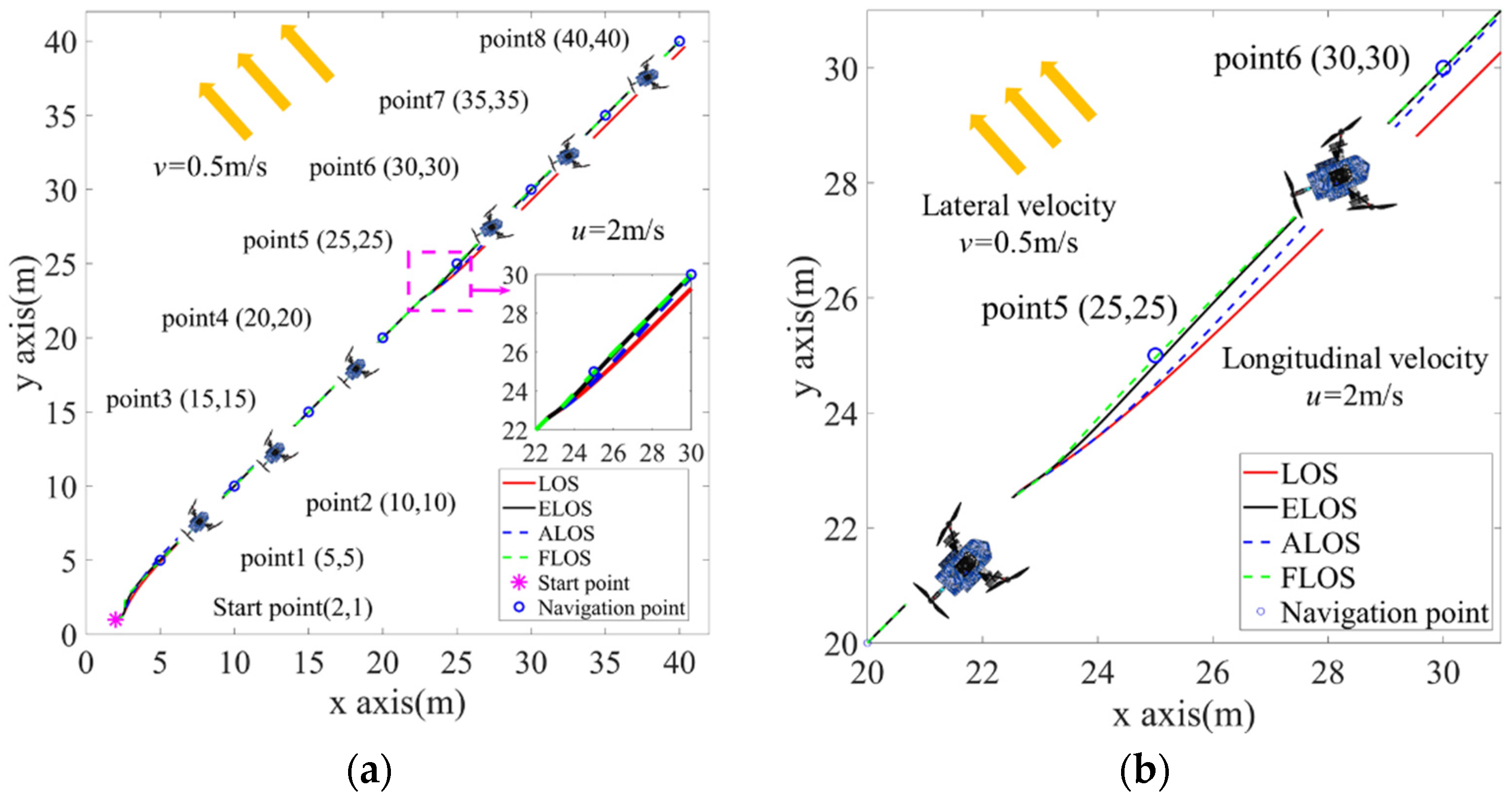
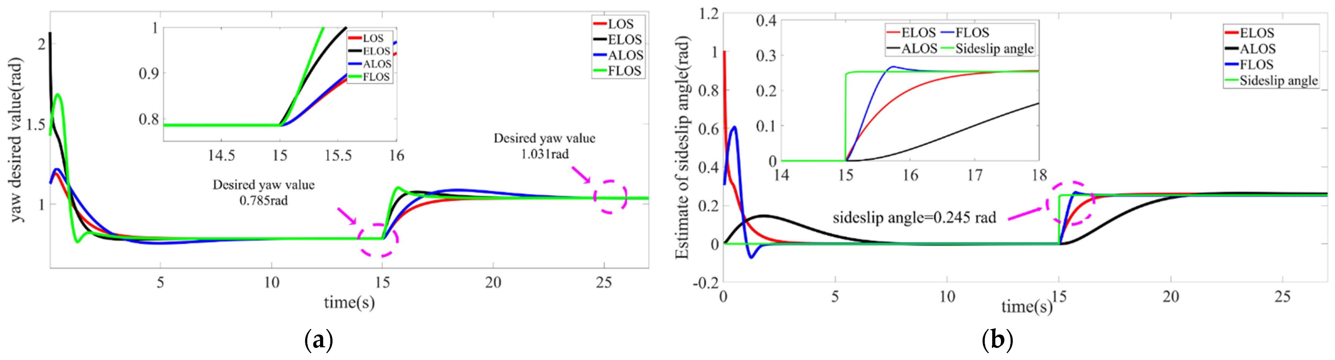
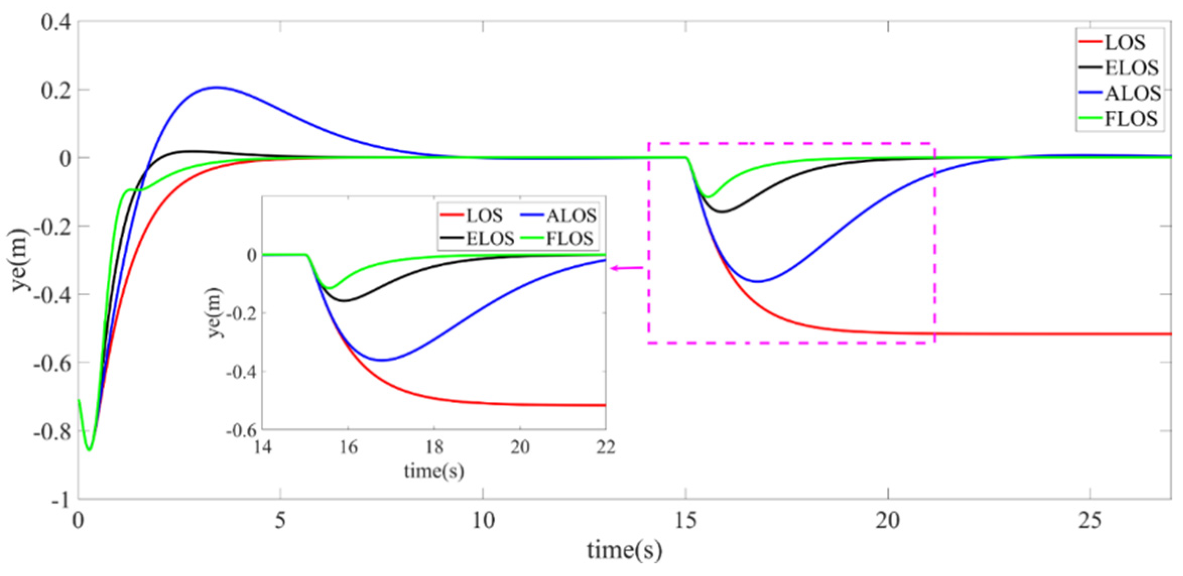
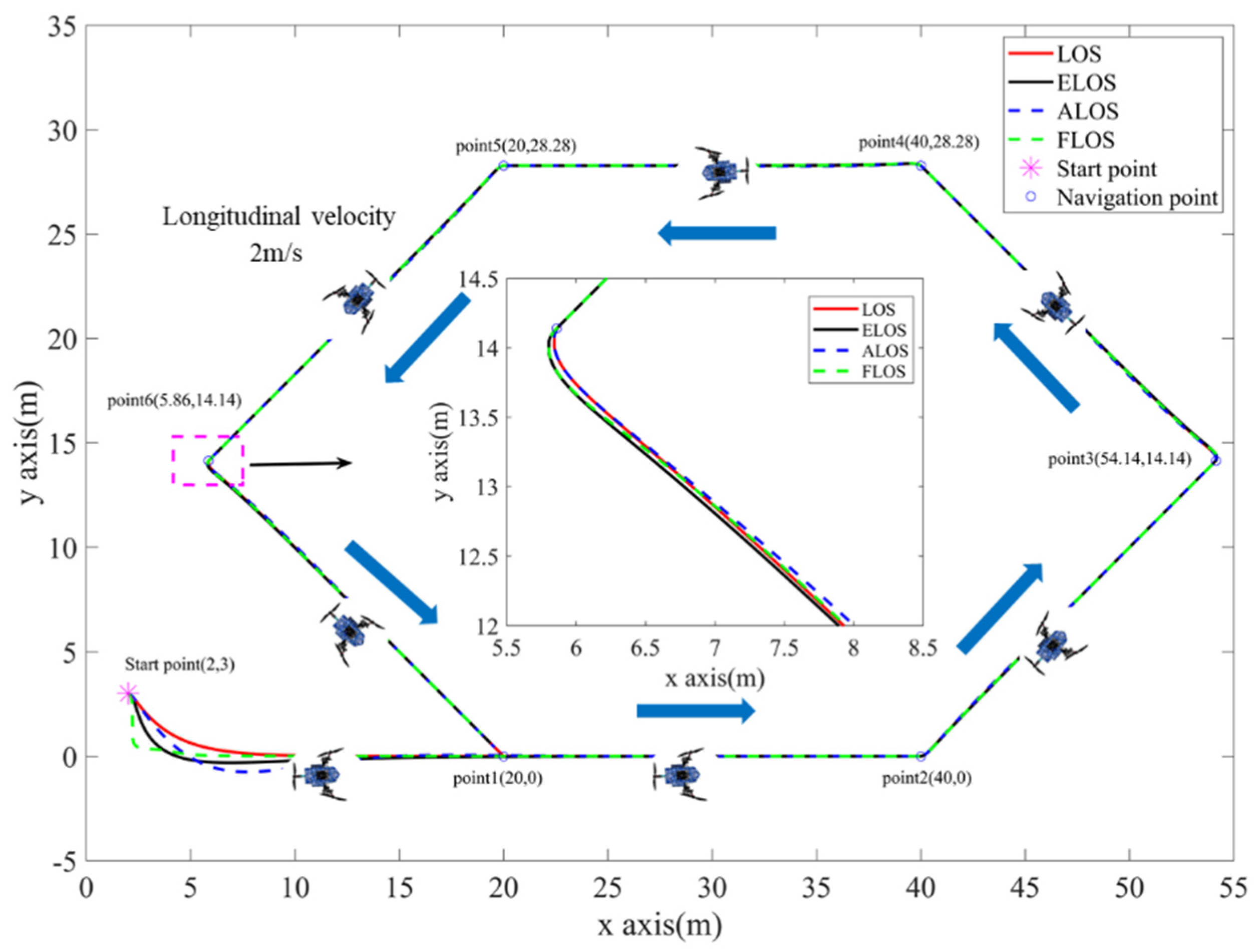
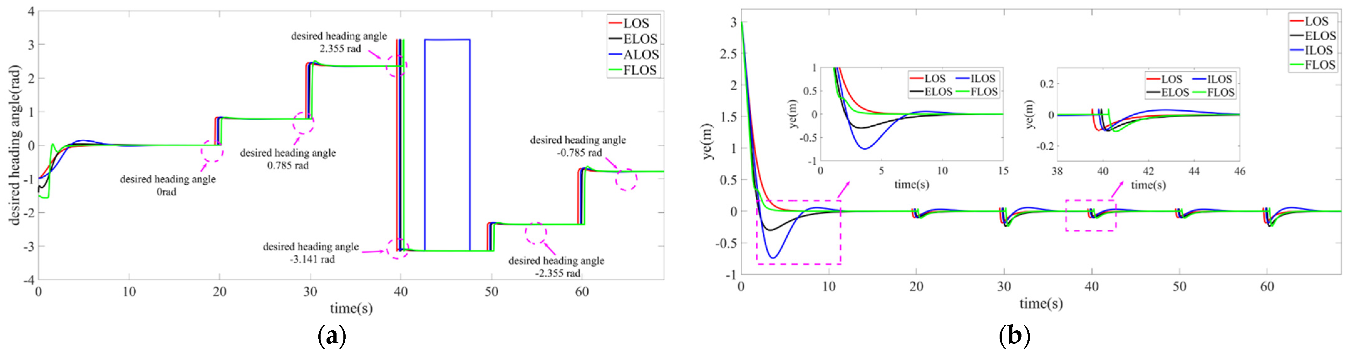
5.1.1. FLOS Navigation Algorithms in Case 1

In Case 1, a straight-line desired trajectory is designed. Additionally, a lateral wind disturbance of v = 0.5 m/s is applied at 15 s. The results can be found in Figure 6, Figure 7 and Figure 8.

In Figure 6, point i (i = 1,2 … 6) is the navigation point. The start point is (2 m, 1 m) and the heading angle is 0 rad. At 15 s, the lateral velocity v = 0.5 m/s is applied to the CDR at position (21.5 m, 21.5 m). In this case, the traditional LOS has a position tracking error that cannot be eliminated as the red line shows. The ELOS, ALOS, FLOS can adjust the yaw angle to eliminate the position error. The heading angle and sideslip angle are shown in Figure 7.

There is no lateral velocity until at 15 s, so the desired heading angle should be 0.785 rad. The FLOS, ELOS, and LOS are all capable of planning the desired heading angle. At 15 s, the lateral velocity v = 0.5 m/s and the longitudinal speed u = 2 m/s, the desired heading angle should be 1.031 rad, a side-slip angle of 0.245 rad appears. ALOS convergence speed is the slowest. The reason is the adaptive rate of ALOS only considers the position error y_e. ELOS considers the position error y_e and x_e, the heading angle error is also introduced into ESO, so it has faster observation speed than ALOS. However, due to the large position error between the current position of the robot with the target position at the initial time, there is a large error in the side-slip angle observed by ELOS at the initial time. FLOS takes the error between y_e with the observed value of y_e as the input state of the side-slip angle observer, so it avoids the large observation error at the initial time. The exponential term is introduced into FLOS algorithm to further improve the planning speed. The position error of y_e as shown in Figure 8.

Without lateral velocity, all four methods can ensure that the position error y_e converges to 0. At 15 s, the lateral velocity appears. Since the traditional LOS algorithm does not consider the lateral velocity, there is a static state error of about 0.5 m that cannot be eliminated. The maximum y_e error of FLOS is about 0.12 m, smaller than that of ELOS (about 0.18 m) and ALOS (about 0.4 m).

To present more clearly the advantages of the FLOS algorithm we have proposed in Case 1, the quantitative comparison is shown in

Table 2. Quantitative comparison of performances for the proposed FLOS with LOS, ALOS, and ELOS in Case 1.

Performance Parameter	LOS	ELOS	ALOS	FLOS
0–15 s, standard deviation ye (m)	0.1843	0.1685	0.2306	0.16
0–15 s, max ye (m)	0	0.018	0.2053	0
Time (s) for ye < 0.01 m in 0–15 s	4.35	4.00	8.49	3.72
15–28 s, standard deviation ye (m)	0.1032	0.0473	0.1322	0.0264
15–28 s max ye (m)	0.5164	0.1588	0.1154	0.3629
Time(s) for ye < 0.01 m in 15–28 s	NAN	4.4970 s	7.404	2.784
0–15 s, time(s) to reach the ideal yaw angle of 0.785 rad	6.3470	6.4910	10.6360	5.7662
15–28 s, time(s) to reach ideal yaw angle 1.031 rad	7.270	6.1650	9.2110	4.9750
0–15 s, yaw angle overshoot 0.785 rad	51.44%	196.66%	55.37%	114.28%
0–15 s, yaw angle overshoot 1.031 rad	0.75%	4.38%	7.08%	5.48%

According to Table 2, the fastest convergence algorithm is the FLOS, which takes 3.72 s for y_e to converge to zero. In the presence of lateral velocity, it takes 2.784 s for y_e converge to zero. The highest tracking accuracy is based on the FLOS, which the standard deviation is 0.16 m in 0–15 s and 0.0264 m in 15–28 s. The time to reach the ideal yaw angle are, respectively, 5.766 s and 4.975 s, which are better than LOS, ELOS and ALOS. However, using FLOS produces overshot in the initial conditions, which is less than using ELOS, but higher than using LOS and ALOS.

.

It should be notes that the continuous parameterized reference trajectory is discretized. Therefore, the time constraint of the desired trajectory is abandoned. The robot should reach the k + 1th navigation point along a straight line from the kth point. The intersection of the robot’s current position and the vertical line of the desired path is taken as the position of the virtual robot, so x_e is always 0. We only discuss the convergence of y_e.

5.1.2. FLOS Navigation Algorithms in Case 2

In Case 2, a more complex scenario hexagonal expectation tracking path is designed. In Case 1, the adaptability of FLOS to the situations with lateral velocity has been verified, so in this scenario lateral velocity will not be imposed. Only the tracking accuracy and the convergence speed of y_e are compared and analyzed. The results can be found in Figure 9 and Figure 10. In Figure 9, the starting point is (2 m, 3 m), and Point I (I = 1…6) is the navigation point.

As shown in Figure 10, after reaching the navigation point, the CDR calculates the desired heading angle to move to the next target point. Since the desired trajectory is regular hexagonal, the desired heading angle is (0, 0.785, 2.355, 3.14 or −3.141, −2.355, −0.785). It should be noted that at 38–50 s, the planned yaw angle is constrained to (−π, π) and the switch from π to −π occurs when it switches from the second quadrant to the third quadrant.

To introduce the advantages of the FLOS algorithm we proposed in the Case 2, the quantitative comparison is shown as

Table 3. Quantitative comparison of performances for the proposed FLOS with LOS, ALOS, and ELOS in Case 2.

Performance Parameter	FLOS	LOS	ALOS	ELOS
Standard deviation ye (m)	0.2780	0.3193	0.3329	0.2942
0–15 s max ye (m)	0	0	0.7443	0.3009
0–15 s ye convergence time (s), (ye < 0.01 m)	4.2190	5.722	11.311	11.286
0–15 s heading angle planning time (s), (abs(ψe) < 0.05 rad)	3.2380	4.4880	7.7780	6.8250
15–70 s ye average convergence time (s)	2.3950	2.4200	3.2040	5.1020
15–70 s mean time (s) for heading angle planning, abs(ψe) < 0.05 rad	4.1810	4.2340	6.9530	5.7670

In Table 3, the y_e standard deviation of FLOS (0.278 m) is the smallest compared with the other three algorithms. Compared to other algorithms, the FLOS algorithm speeds up the convergence speed because it introduces the exponential term of the position error for planning heading angle.

.

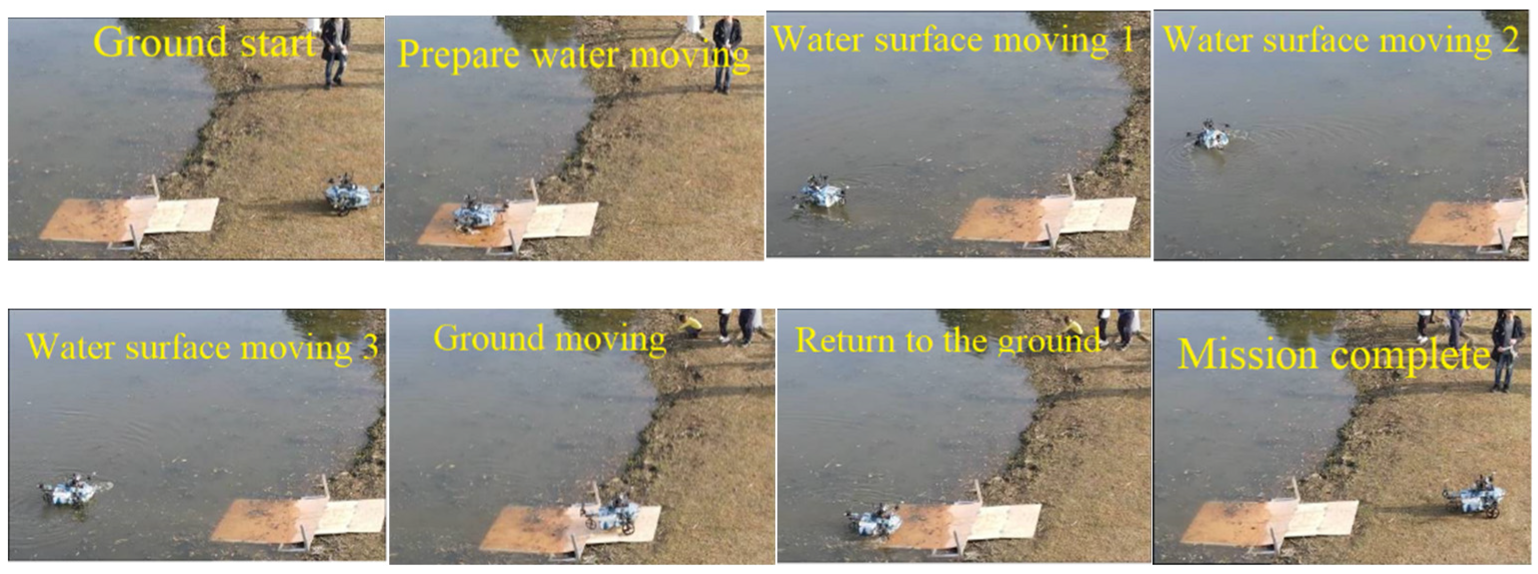
5.2. The Results of CDR Movement on the Ground and the Water Surface

The FLOS algorithm is used to plan the yaw angle and the linear velocity for the robot. It is necessary to design a controller for the robot to track the desired yaw angle and linear velocity. To verify the effectiveness of the proposed control algorithm, the proposed ASMIBC is applied to an ideal second-order system, such as Equation (27). There is no unknown and uncertain disturbance in the system from 0 to 20 s. At 20 s, the second-order state of the system is subjected to a step disturbance with a value of 3. The control results are compared with PID, SMC and IBC, and the results are shown in Figure 11, Figure 12 and Figure 13.

As shown in Figure 10. The desired state of 1 is a constant, IBC loses ability to constrain the system state as shown by the pink line. The static error of SMC is smaller than that of IBC, which is about 1.5. However, the gain of the sliding surface is a fixed constant and the robustness of the controller is limited. The PID control has an integral term, the error can converge slowly, while it also has the same maximum tracking error as IBC. Our proposed ASMIBC has a static error of about 0.05 when there is no adaptive compensation (the blue line). As we design an adaptive sliding surface gain, the closer the system state is to the set boundary, the larger the sliding surface gain will be. Therefore, the robustness of the controller is improved. When adaptive compensation exists, our proposed control method (the red line) can ensure the error convergence is achieved within 6 s. The gain of sliding mode surface is shown in Figure 12.

The robustness of SMC can be improved by increasing the gain of the switching function, but if the gain is too large, the system state will tremble. Our proposed method can adaptively adjust the gain of sliding mode switching function. When there is no disturbance, the gain will be 0, and the gain will be adjusted in 20 s to suppress the influence of step disturbance on the system. However, when the ASMICB has adaptive compensation, a large sliding mode gain is not required, so the chattering of the state can be reduced. The adaptive output of ASMIBC with adaptive compensation is shown in Figure 13.

The linear velocity of the robot moves on the ground is 2 m/s, and the linear velocity of the robot moves on the water surface is 1 m/s. To simulate the robot moving from the ground to the water surface, when the robot moves on the ground, the acceleration is subjected to a random disturbance with an average value −0.5 m/s², which is used to simulate the lumped disturbance caused by air resistance and mechanical loss. At 15 s, the robot moves from the ground to the water surface, the acceleration is subjected to a random disturbance with an average value −3 m/s², which is used to simulate the lumped disturbance caused by water resistance, water flow and the uncertain model parameters. The control result is shown in Figure 14.

From 0 s to 15 s, the robot moves on the ground, all control methods except IBC can track the desired linear velocity of 2 m/s. This is because IBC is a model-based control method, and its robustness is weaker than other control methods. At 15 s, the robot reaches the water surface, the desired velocity speed of the robot is 1 m/s. Our proposed control method can track the desired linear speed, as shown by the red line. Without adaptive rate compensation, ASMIBC has a static error of about 0.05 m/s. The adaptive compensation and the adaptive sliding mode gain have been discussed in Figure 12 and Figure 13, so they are not introduced here.

The yaw angle of the robot on the water surface and the ground does not need to be constrained. Constraints on the yaw angular velocity are required to prevent the drive from saturating or the robot from being placed in a dangerous condition due to a large yaw angular velocity. The yaw angle control results on the ground is shown in Figure 15.

In Figure 15, the desired yaw angle is −1 rad at 0 s and 1 rad at 15 s. A random disturbance with a mean value of 5 rad/s/s is applied to the acceleration of the yaw angle to simulate the impact of lumped uncertain disturbance on the system. Our proposed algorithm can control the actual yaw angle to follow the desired yaw angle. The angle control results of SMC, PID and IBC are shown in Figure 15b. Both PID and ASMIBC can follow the desired yaw angle. There is a static error of 0.3 rad in SMC and 0.4 rad in IBC. The yaw angular velocity control is shown in Figure 16 and Figure 17.

As shown in Figure 16a, the maximum yaw angular velocity is 2.5 rad/s. Our proposed control method can follow the desired yaw angular velocity without overshoot and without exceeding the set boundary of 2.6 rad/s. The results of the other four control methods are shown in Figure 16b. Without the adaptive compensation, ASMIBC has a static error of about 0.1 rad/s, but it does not exceed the set boundary of 2.6 rad/s. As mentioned before, our proposed ASMIBC can adaptively adjust the gain of the sliding surface to suppress the disturbance, but it cannot eliminate the influence of the disturbance in the system state. ASMIBC with adaptive compensation can completely eliminate the effect of the disturbance in the system. SMC and PID cannot constrain the yaw angular velocity, the actual yaw angular velocity exceeds the set boundary by 2.6 rad/s. Since the boundary constraint is considered in the algorithm, traditional IBC can constrain the yaw angular velocity from exceeding the set boundary. However, IBC is a model-based control method, so it cannot solve the problems caused by model uncertainty. Due to the static error of angular velocity control, the actual heading angle cannot follow the desired heading angle. Adaptive compensation and adaptive sliding mode gain are shown in Figure 17.

The desired yaw angle is 1 rad/s, and the desired yaw angle is −1 rad/s at 15 s. The yaw angle control of the robot on the water surface is shown in Figure 18:

As shown in Figure 18a, the robot can follow the desired yaw angle with our proposed control method, and ASMIBC can also follow the desired yaw angle without the adaptive rate compensation. However, the robot tracking the desired yaw angle with SMC and IBC has a static error of about 0.2 rad, and PID control can track the desired yaw angle, but the tracking error takes a long time to converge.

The maximum desired angular velocity of the robot on the water surface is 1.5 rad/s, and a random disturbance with an average value −5 rad/s/s is applied to the angular acceleration of the robot to simulate the water resistance and wind disturbance encountered by the robot when moves on the water surface. Yaw angular velocity control is shown in Figure 19.

The controller of the robot adopts the same control parameters on the ground and the water surface. The ASMIBC and ASMIBC with the adaptive compensation proposed by us can ensure the robot to track the desired angular velocity and do not exceed the set boundaries. The adaptive output compensation and adaptive sliding surface have been discussed in the previous results, so they are not presented here.

6. Conclusions

In this paper, a FLOS algorithm without considering the small angle assumption is proposed. FESO is used to obtain the side-slip angle caused by the lateral velocity and to compensate the yaw angle output of FLOS. To make the robot follow the desired speed and yaw angle, an ASMIBC is proposed. Our proposed control method solves the problem that the traditional IBC loses its ability to constrain the system state when the desired speed and the desired angular velocity are constant. The adaptive sliding mode gain reduces the influence of uncertain lumped disturbances on the robot, improve the robustness of the robot and constrain the state of the system. The adaptive rate compensates the output of ASMIBC to further improve the adaptability of the system. By comparing with other LOS algorithms and control methods, the effectiveness of our proposed control algorithm is verified.

For further research, the constraint boundary of barrier control is a strong constraint. When the system state exceeds the constraint boundary, the control system is unstable. Therefore, we need to consider a boundary control algorithm with soft constraints.

References

1. Guo, J.; Zhang, K.; Guo, S.; Li, C.; Yang, X. Design of a New Type of Tri-habitat Robot. In Proceedings of the 2019 IEEE International Conference on Mechatronics and Automation (ICMA), Tianjin, China, 4–7 August 2019; IEEE: Piscataway, NJ, USA, 2019; pp. 1508–1513. [Google Scholar]
2. Tan, Q.; Zhang, X.; Liu, H.; Jiao, S.; Zhou, M.; Li, J. Multimodal Dynamics Analysis and Control for Amphibious Fly-Drive Vehicle. IEEEASME Trans. Mechatron. 2021, 26, 621–632. [Google Scholar] [CrossRef]
3. Li, Y.; Lu, H.; Nakayama, Y.; Kim, H.; Serikawa, S. Automatic road detection system for an air–land amphibious car drone. Future Gener. Comput. Syst. 2018, 85, 51–59. [Google Scholar] [CrossRef]
4. Yang, Y.; Zhou, G.; Zhang, J.; Cheng, S.; Fu, M. Design, modeling and control of a novel amphibious robot with dual-swing-legs propulsion mechanism. In Proceedings of the 2015 IEEE/RSJ International Conference on Intelligent Robots and Systems (IROS), Hamburg, Germany, 28 September–2 October 2015; IEEE: Piscataway, NJ, USA, 2015; pp. 559–566. [Google Scholar]
5. Liu, H.; Shi, L.; Guo, S.; Xing, H.; Hou, X.; Liu, Y. Platform Design for a Natatores-like Amphibious robot. In Proceedings of the 2018 IEEE International Conference on Mechatronics and Automation (ICMA), Changchun, China, 5–8 August 2018; IEEE: Piscataway, NJ, USA, 2018; pp. 1627–1632. [Google Scholar]
6. Zhong, B.; Zhang, S.; Xu, M.; Zhou, Y.; Fang, T.; Li, W. On a CPG-Based Hexapod Robot: AmphiHex-II with Variable Stiffness Legs. IEEEASME Trans. Mechatron. 2018, 23, 542–551. [Google Scholar] [CrossRef]
7. Guo, S.; He, Y.; Shi, L.; Pan, S.; Xiao, R.; Tang, K.; Guo, P. Modeling and experimental evaluation of an improved amphibious robot with compact structure. Robot. Comput.-Integr. Manuf. 2018, 51, 37–52. [Google Scholar] [CrossRef]
8. Li, M.; Guo, S.; Hirata, H.; Ishihara, H. A roller-skating/walking mode-based amphibious robot. Robot. Comput.-Integr. Manuf. 2017, 44, 17–29. [Google Scholar] [CrossRef]
9. Lauder, G.V. Flight of the robofly. Nature 2001, 412, 688–689. [Google Scholar] [CrossRef]
10. Chukewad, Y.M.; James, J.; Singh, A.; Fuller, S. RoboFly: An insect-sized robot with simplified fabrication that is capable of flight, ground, and water surface locomotion. arXiv 2020, arXiv:2001.02320. [Google Scholar] [CrossRef]
11. Huang, C.; Liu, Y.; Wang, K.; Bai, B. Land–Air–Wall Cross-Domain Robot Based on Gecko Landing Bionic Behavior: System Design, Modeling, and Experiment. Appl. Sci. 2022, 12, 3988. [Google Scholar] [CrossRef]
12. Meiri, N.; Zarrouk, D. Flying STAR, a Hybrid Crawling and Flying Sprawl Tuned Robot. In Proceedings of the 2019 International Conference on Robotics and Automation (ICRA), Montreal, QC, Canada, 20–24 May 2019; IEEE: Piscataway, NJ, USA, 2019; pp. 5302–5308. [Google Scholar]
13. Cohen, A.; Zarrouk, D. The AmphiSTAR High Speed Amphibious Sprawl Tuned Robot: Design and Experiments. In Proceedings of the 2020 IEEE/RSJ International Conference on Intelligent Robots and Systems (IROS), Las Vegas, NV, USA, 24 October 2020–24 January 2021; IEEE: Piscataway, NJ, USA, 2021; pp. 6411–6418. [Google Scholar]
14. Elmokadem, T.; Zribi, M.; Youcef-Toumi, K. Trajectory tracking sliding mode control of underactuated AUVs. Nonlinear Dyn. 2016, 84, 1079–1091. [Google Scholar] [CrossRef]
15. Liao, Y.; Zhang, M.; Wan, L.; Li, Y. Trajectory tracking control for underactuated unmanned surface vehicles with dynamic uncertainties. J. Cent. South Univ. 2016, 23, 370–378. [Google Scholar] [CrossRef]
16. Gonzalez-Garcia, A.; Castaneda, H. Guidance and Control Based on Adaptive Sliding Mode Strategy for a USV Subject to Uncertainties. IEEE J. Ocean. Eng. 2021, 46, 1144–1154. [Google Scholar] [CrossRef]
17. Guo, Y.; Yu, L.; Xu, J. Robust Finite-Time Trajectory Tracking Control of Wheeled Mobile Robots with Parametric Uncertainties and Disturbances. J. Syst. Sci. Complex. 2019, 32, 1358–1374. [Google Scholar] [CrossRef]
18. Liu, K.; Gao, H.; Ji, H.; Hao, Z. Adaptive Sliding Mode Based Disturbance Attenuation Tracking Control for Wheeled Mobile Robots. Int. J. Control Autom. Syst. 2020, 18, 1288–1298. [Google Scholar] [CrossRef]
19. Li, Z.; Yang, C.; Su, C.-Y.; Deng, J.; Zhang, W. Vision-Based Model Predictive Control for Steering of a Nonholonomic Mobile Robot. IEEE Trans. Control Syst. Technol. 2015, 24, 553–564. [Google Scholar] [CrossRef]
20. Zhou, W.; Wang, Y.; Ahn, C.K.; Cheng, J.; Chen, C. Adaptive Fuzzy Backstepping-Based Formation Control of Unmanned Surface Vehicles with Unknown Model Nonlinearity and Actuator Saturation. IEEE Trans. Veh. Technol. 2020, 69, 14749–14764. [Google Scholar] [CrossRef]
21. Zhao, Y.; Qi, X.; Ma, Y.; Li, Z.; Malekian, R.; Sotelo, M.A. Path Following Optimization for an Underactuated USV Using Smoothly-Convergent Deep Reinforcement Learning. IEEE Trans. Intell. Transp. Syst. 2021, 22, 6208–6220. [Google Scholar] [CrossRef]
22. Gheisarnejad, M.; Khooban, M.H. An Intelligent Non-Integer PID Controller-Based Deep Reinforcement Learning: Implementation and Experimental Results. IEEE Trans. Ind. Electron. 2021, 68, 3609–3618. [Google Scholar] [CrossRef]
23. Yang, H.; Guo, M.; Xia, Y.; Sun, Z. Dual closed-loop tracking control for wheeled mobile robots via active disturbance rejection control and model predictive control. Int. J. Robust Nonlinear Control 2020, 30, 80–99. [Google Scholar] [CrossRef]
24. Li, X.; Ren, C.; Ma, S.; Zhu, X. Compensated model-free adaptive tracking control scheme for autonomous underwater vehicles via extended state observer. Ocean Eng. 2020, 217, 107976. [Google Scholar] [CrossRef]
25. Guo, Y.; Qin, H.; Xu, B.; Han, Y.; Fan, Q.-Y.; Zhang, P. Composite learning adaptive sliding mode control for AUV target tracking. Neurocomputing. 2019, 351, 180–186. [Google Scholar] [CrossRef]
26. Xia, Y.; Xu, K.; Li, Y.; Xu, G.; Xiang, X. Improved line-of-sight trajectory tracking control of under-actuated AUV subjects to ocean currents and input saturation. Ocean Eng. 2019, 174, 14–30. [Google Scholar] [CrossRef]
27. Ali, N.; Tawiah, I.; Zhang, W. Finite-time extended state observer based nonsingular fast terminal sliding mode control of autonomous underwater vehicles. Ocean Eng. 2020, 218, 108179. [Google Scholar] [CrossRef]
28. Liu, Y.-J.; Tong, S. Barrier Lyapunov Functions-based adaptive control for a class of nonlinear pure-feedback systems with full state constraints. Automatica 2016, 64, 70–75. [Google Scholar] [CrossRef]
29. Ames, A.D.; Coogan, S.; Egerstedt, M.; Notomista, G.; Sreenath, K.; Tabuada, P. Control Barrier Functions: Theory and Applications. In Proceedings of the 2019 18th European Control Conference (ECC), Naples, Italy, 25–28 June 2019; IEEE: Piscataway, NJ, USA, 2019; pp. 3420–3431. [Google Scholar]
30. Li, L.; Dong, K.; Guo, G. Trajectory tracking control of underactuated surface vessel with full state constraints. Asian J. Control. 2021, 23, 1762–1771. [Google Scholar] [CrossRef]
31. Cruz-Ortiz, D.; Chairez, I.; Poznyak, A. Non-singular terminal sliding-mode control for a manipulator robot using a barrier Lyapunov function. ISA Trans. 2021, 121, 268–283. [Google Scholar] [CrossRef] [PubMed]
32. Liu, L.; Gao, T.; Liu, Y.-J.; Tong, S.; Chen, C.L.P.; Ma, L. Time-varying IBLFs-based adaptive control of uncertain nonlinear systems with full state constraints. Automatica 2021, 129, 109595. [Google Scholar] [CrossRef]
33. Fu, M.; Zhang, T.; Ding, F. Adaptive Safety Motion Control for Underactuated Hovercraft Using Improved Integral Barrier Lyapunov Function. Int. J. Control Autom. Syst. 2021, 19, 2784–2796. [Google Scholar] [CrossRef]
34. Liu, L.; Wang, D.; Peng, Z. ESO-Based Line-of-Sight Guidance Law for Path Following of Underactuated Marine Surface Vehicles with Exact Sideslip Compensation. IEEE J. Ocean. Eng. 2017, 42, 477–487. [Google Scholar] [CrossRef]
35. Wang, N.; Ki Ahn, C. Hyperbolic-Tangent LOS Guidance-Based Finite-Time Path Following of Underactuated Marine Vehicles. IEEE Trans. Ind. Electron. 2020, 67, 8566–8575. [Google Scholar] [CrossRef]
36. Yu, Y.; Guo, C.; Li, T. Finite-time LOS Path Following of Unmanned Surface Vessels with Time-varying Sideslip Angles and Input Saturation. IEEEASME Trans. Mechatron. 2021, 27, 463–474. [Google Scholar] [CrossRef]
37. Fossen, T.I.; Pettersen, K.Y.; Galeazzi, R. Line-of-Sight Path Following for Dubins Paths with Adaptive Sideslip Compensation of Drift Forces. IEEE Trans. Control Syst. Technol. 2015, 23, 820–827. [Google Scholar] [CrossRef]
38. Hou, Q.; Ding, S. Finite-time Extended State Observer Based Super-twisting Sliding Mode Controller for PMSM Drives with Inertia Identification. IEEE Trans. Transp. Electrif. 2021, 8, 1918–1929. [Google Scholar] [CrossRef]
39. Zhu, Z.; Xia, Y.; Fu, M. Attitude stabilization of rigid spacecraft with finite-time convergence: Attitude Stabilization of Rigid Spacecraft. Int. J. Robust Nonlinear Control 2011, 21, 686–702. [Google Scholar] [CrossRef]
40. Tee, K.P.; Ge, S.S. Control of state-constrained nonlinear systems using Integral Barrier Lyapunov Functionals. In Proceedings of the 2012 IEEE 51st IEEE Conference on Decision and Control (CDC), Maui, HI, USA, 10–13 December 2012; IEEE: Piscataway, NJ, USA, 2013; pp. 3239–3244. [Google Scholar] [CrossRef]
41. Xia, J.; Zhang, J.; Sun, W.; Zhang, B.; Wang, Z. Finite-time adaptive fuzzy control for nonlinear systems with full state constraints. IEEE Trans. Syst. Man Cybern. Syst. 2019, 49, 1–8. [Google Scholar] [CrossRef]
Figure 1. The structure and actuators of the CDR. (a) The structure of the CDR. (b) The actuators of the CDR. The CDR uses three motors in the air and two motors on the ground and the water surface.
Applsci 12 05935 g001
Figure 2. The main sensors and controllers of CDR. From bottom to top, the first layer is the power supply layer for generating 5 v, 7.4 v and 24 v voltages. The second layer is the main control layer, from which the driving signal of the motor is output. The third layer is the sub-controller layer, which is used to collect messages of the sensors. The fourth and fifth layers are the sensor layers, where the sensors used by the robot are placed.
Applsci 12 05935 g002
Figure 3. The CDR moves on the water surface and the ground. The robot follows the desired trajectory from the ground and returns to the starting navigation point after reaching the navigation point on the water surface.
Applsci 12 05935 g003
Figure 4. CDR in Frenet–Secret frame. xe and ye are error between current position of the robot and the desired position.
Applsci 12 05935 g004
Figure 5. Control structure of the CDR on the ground and water surface. FLOS is used to plan the yaw angle and linear velocity of the robot. Speed controller and yaw angle controller are used to track the desired yaw angle and linear velocity.
Applsci 12 05935 g005
Figure 6. Four LOS methods are used to track the desired path. (a) CDR tracks eight navigation points. (b) Tracking the desired path with the lateral velocity v = 0.5 m/s. At 15 s, the lateral velocity v = 0.5 m/s is applied to the CDR, which caused side-slip angle.
Applsci 12 05935 g006
Figure 7. The desired heading angle is planned by the four LOS algorithms. (a) Desired heading angle. The desired heading is 0.785 rad when there is no lateral velocity. (b) Side-slip angle. The side-slip angle is 0.245 rad when there is lateral velocity v = 0.5 m/s.
Applsci 12 05935 g007
Figure 8. Position error ye. The traditional LOS algorithm does not consider the lateral velocity. Therefore, there is a static state error of about 0.5 m that cannot be eliminated.
Applsci 12 05935 g008
Figure 9. Tracking a hexagonal desired trajectory. The robot follows the hexagonal desired trajectory to the navigation points one by one.
Applsci 12 05935 g009
Figure 10. Heading angle and position error ye of the CDR. (a) Heading angle changes when robot tracks the desired trajectory. (b) The CDR hexagonal trajectory tracking of ye.
Applsci 12 05935 g010
Figure 11. ASMIBC for an ideal second-order control model. Only the proposed algorithm can track the desired value 1. As the adaptive rate is designed in the ASMIBC, there is no static error.
Applsci 12 05935 g011
Figure 12. ASMIBC adaptive sliding mode gain. (a) ASMIBC without adaptive compensation. Our proposed method can adaptively adjust the gain of sliding mode. When there is no disturbance, the gain will be 0, and the gain will increase when the system is influenced by disturbance. (b) ASMIBC with adaptive compensation. With the ASMICB has adaptive compensation, a large sliding mode gain is not required.
Applsci 12 05935 g012
Figure 13. ASMIBC adaptive compensation output. The second-order state of the system is subjected to a step disturbance with a value of 3. The disturbance of the system can be obtained through the adaptive rate.
Applsci 12 05935 g013
Figure 14. Velocity control of CDR on the ground and water surface. From 0 s to 15 s, the robot moves on the ground, the desired velocity of the robot is 2 m/s. At 15 s, the robot reaches the water surface, the desired velocity of the robot on the water surface is 1 m/s.
Applsci 12 05935 g014
Figure 15. Robot heading angle control on the ground. (a) The control result of proposed method. (b) The other four control method results. The initial desired heading angle of the robot is −1 rad. At 15 s, the desired heading angle is 1 rad.
Applsci 12 05935 g015
Figure 16. Yaw angular velocity control of robot on the ground. (a) The control result of proposed method. (b) The other four control method results. The maximum yaw angular velocity is 2.5 rad/s. Only the control algorithm considering boundary constraints can ensure the yaw angle velocity does not exceed the set boundary. Such as, ASMIBC and IBC.
Applsci 12 05935 g016
Figure 17. Adaptive compensation output and adaptive sliding mode gain. (a) Adaptive compensation output of the angular velocity controller. The robot is subjected to lumped disturbance of 5 m/s/s on the water surface, and the designed adaptive rate can obtain the lumped disturbance. (b) Adaptive sliding mode gain of the angular velocity controller. Due to adaptive compensation, the sliding mode gain is 0 even if there exists a lumped disturbance.
Applsci 12 05935 g017
Figure 18. Robot heading angle control on the water surface. (a) The control result of proposed method. (b) The other four control method results. The initial desired heading angle of the robot is 1 rad. At 15 s, the desired heading angle is −1 rad.
Applsci 12 05935 g018
Figure 19. Angular velocity control of the robot on the water surface. (a) The control result of proposed method. (b) The other four control method results. There is a limit to the control input of the robot. In this case, the traditional IBC cannot constrain the robot’s angular velocity. Although this problem can be solved by reducing the gain of IBC controller. However, to compare the control results of different control algorithms, we use the same controller parameters on the ground and the water surface.
Applsci 12 05935 g019