1. Introduction
Nowadays, robotics has several areas, each of which is closely related. The area of robotics that we focus on in our workplace is called Simultaneous Localization and Mapping (SLAM). In solving this problem, the robotic system is in an unknown environment, and the initial position is known. The main goals of the SLAM solution are to obtain the most accurate model of the mapped environment and to monitor the exact position of the robotic system in the environment. This task does not seem very difficult when considering an ideal environment where various noises and measurement errors do not occur. Unfortunately, this kind of environment can only be achieved on a theoretical level. Various types of methods and algorithms are used to overcome these shortcomings. The sequence of individual steps is generally still the same and independent of the type of algorithm used. The steps are as follows: initialization, data association, extraction of landmarks, estimation of the state of the mobile robotic system and the state of landmarks, updating the status of the mobile robotic system, and updating the status of landmarks. For each of the mentioned steps, it is possible to use different solution methods, which are already linked to the specific algorithm used. SLAM can be used in a variety of environments, whether on land, in water, or in the air. Currently, one of the most popular techniques in this area is called ASLAM. It is often referred to in the scientific literature as automatic SLAM [
1], autonomous SLAM [
2], or SPLMA (Simultaneous Planning, Localization and Mapping) [
3]. All these mentioned names have the same destination and thus is active motion selection. Using ASLAM, the autonomous movement of the mobile robotic system is solved in order to obtain a map. In the obtained map, various areas of our interest can be defined, such as unexplored areas, areas of irregular shapes, and areas with narrow alleys. The topic of autonomous vehicles is very wide. If we wanted to focus on the field of road transport, we could have achieved it as the author in [
4] did, where he chose to use LAS (Lane Assistant System) technology. If we wanted to transfer such an application to the field of industry, it is possible to cite the deployment of an Autonomous Ground Vehicle (AGV) in an industrial hall as an example. It is usually necessary to map the space before deployment (this depends on the technology used), and it is possible to use active SLAM for this. Such mapping is often performed during working hours and the customer cannot always afford to be absent from the workforce, with the result that there may be a dynamic object in the mapped environment in the form of moving people. This can result in defects in the map and collisions of the robotic system with a dynamic object. We considered these mentioned complications to be crucial from our point of view, so we tried to find a solution. ASLAM with a combination of dynamic object detection to avoid collisions can significantly reduce the time required to map the environment.
When operating a mobile robotic system, the detection of dynamic objects in the environment is an important aspect that increases the safety of the entire system. However, detection alone is often not enough to provide reliable navigation in a complex environment. The ideal situation is if the robotic system can predict the shape and trajectory of the movement in order to avoid collisions. The combination of dynamic object motion detection and prediction can be considered a particularly challenging task if we consider the variability of dynamic object patterns. Taking into account as an example two objects: a man and a car, two different types of motion arise. The person moves nonlinearly and without significant restrictions when changing direction, while the car has a smoother movement and reaches a much higher speed, which can cause a problem when tracking it. Even with this consideration, it can be seen that this is a complex problem in which a different approach to the solution can be chosen. If an algorithm is used to map a dynamic environment that does not consider the occurrence of dynamic objects, it will adversely affect the mapping result. This has resulted in new methods and approaches to addressing SLAM. Detection and tracking of moving objects (DATMO) deals with the detection and tracking of dynamic objects. This issue is relatively old and the author has summarized it in [
5], summarizing the current state and possible methods of solution. In [
6], the author focused on the creation of a probabilistic technique of data clustering and estimation of the movement of individual clusters. He called this method CRF-Clustering (Conditional Random Fields). In addition, he addressed the issue of overlapping points of dynamic objects in individual consecutive images. He performed the measurements by scanning the environment using a 2D lidar. The problem of creating a map in a dynamic environment is addressed by the author in [
7]. In the article, the author designs a new method that inserts a probabilistic technique for identifying false measurements between mapping and localization processes. The aim of his work was to capture dynamic objects, isolate them, and represent them in 3D space using lidar scanning. In this approach, he worked with both 2D and 3D lidar data. In the mentioned sources, the authors mainly focused on the detection of a dynamic object, or its tracking or removal from the map.
One of the interesting options for accessing detected dynamic objects can take advantage of the autonomous movement of the robot. If the robot detects the occurrence of a dynamic object in its motion trajectory, it recalculates a new trajectory that would dynamically reflect the object on the map. This mentioned issue was an area of our interest. One of the first steps was to design an algorithm that would allow the detection of dynamic objects. During the designing process, we decided to use a method that is based on the scan matching. Scan matching is the process of obtaining the relative pose between two frames whose visual fields overlap with one another. This method is often used when solving SLAM. A high-precision frame-to-frame scan matching algorithm is critical to improve the autonomous navigation capabilities of robots. Scan matching algorithms can be divided into two categories based on the type of sensor used: laser scan matching algorithms and visual scan matching algorithms. Compared to visual sensors, laser lidar has anti-interference capabilities, and its performance is not affected by light. Moreover, the research results of this paper were applied to indoor service robots, so 2D lidar sensors were adopted for scan matching. Due to the importance of the frame-to-frame scan matching algorithm, it has attracted much research attention, and research has resulted in many milestone findings. The most classic frame-to-frame scan matching algorithm is the Iterative Closest Point (ICP) algorithm proposed in [
8]. A large number of variants [
9] have been proposed based on ICP. Authors in [
10] proposed Point-to-Line ICP (PL-ICP), which overcomes the shortcomings of low-resolution lidar data and has quadratic convergence properties, achieving fewer iterations and higher accuracy, and this algorithm performed well in a structured environment. Similar to the PL-ICP, [
11] proposed a probabilistic version of the ICP: GICP (Generalized ICP), which uses the Gaussian distribution to model the lidar sensor data and assigns weights according to the normal vector. This algorithm can be considered to be a variant of Point-to-Plane ICP [
12]. The authors in [
13] introduced a frame-to-frame Scan Matching Algorithm for 2D Lidar Based on Attention. This method took into account only a part of the images in the comparison, which guaranteed less error accumulation and higher accuracy. We were most interested in the SegMatch method described in [
14]. The SegMatch algorithm was designed for online real-time loop closure detection and localization. We decided to use part of this method in our design. The result of these methods should be to estimate the position of individual images based on matching areas, with nonmatching areas becoming irrelevant. In the approach proposed in this article, we focus on nonmatching areas and try to verify that these are dynamic objects.
Section 2 discusses the used hardware and software.
Section 3 deals with the design and implementation of an algorithm for detecting dynamic objects during SLAM execution.
2. Hardware and Software Solutions
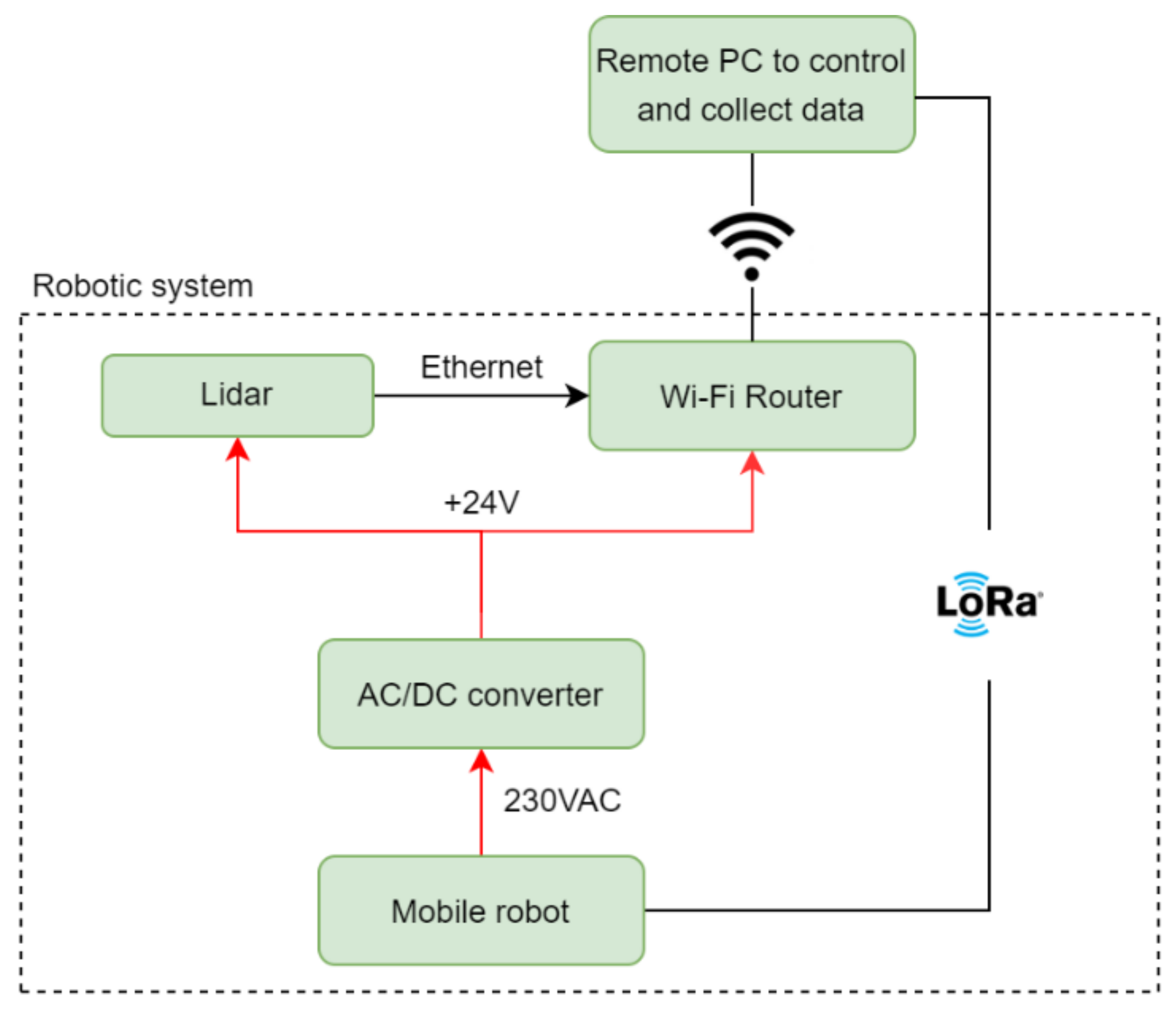
For practical validation of the mentioned issue, it is necessary to have a mobile robotic system (MRS), to which the proposed solution can be applied. From our point of view, the MRS used is considered a black box that can be controlled using the API. Communication with the robot takes place using LoRa technology. LoRa (Long Range) is a spread spectrum modulation technique derived from chirp spread spectrum technology. This technology is a long-range, low-power wireless platform that has become the de facto wireless platform of the Internet of Things. A Lidar LD-OEM 1000 is mounted on the MRS, which performs measurements. LoRa communication technology does not allow sending data in the volume and speed required, so a Wi-Fi router is added, which communicates with lidar and an external computing unit using the TCP/IP protocol. The concept is summarized in
Figure 1. The main element of this robotic system is the omnidirectional wheels. If omnidirectional wheels and a relevant control algorithm are used, then the robotic system is holonomic. The design and execution of this MRS is beyond the scope of this article and will therefore be published in our future publications.
There are currently many open-source solutions for SLAM, so we do not consider it necessary to make new ones. We decide to use the Matlab platform, which offers its algorithm and adapts it on our own. Matlab uses the collaboration of several libraries for the SLAM solution, while the Robotic toolbox, Computer vision, Lidar toolbox, and Navigation toolbox already include specific solutions. It is possible to map the environment using a lidar sensor, RGB camera, but also using an IMU. How the algorithm works is discussed in [
15,
16]. Testing the SLAM algorithm on MRS is only the first step in creating the entire ASLAM algorithm. The second step is to choose a suitable target for the next move of the MRS. The topic of ASLAM is beyond the scope of this article. If the destination to which the MRS is to be moved is selected, we can use the path planning algorithm. The next chapter focuses on path planning algorithms.
2.1. Path Planning
Path planning is a term known in robotics as part of the navigation of an autonomous robot. The result of planning is the process by which we go from the initial position to the target position. The main condition is that the road does not cross with objects in the area. There are two approaches to path planning, local or global planning. Global trip planning is based on a familiar environment and is suitable for finding the optimal route. In local planning, the robot responds appropriately to unknown or dynamic obstacles. In this case, the robot makes decisions while moving. By combining both methods, better results can be achieved. The planning can be divided into two parts, while each part can be solved separately. The first deals with the pre-processing of the workspace, where this space is discretized and then converted into a configuration space. The configuration space consists of all robot configurations in the workspace where it performs the given tasks. The robot configuration is determined by a vector that contains the position and orientation of the robot. After discretizing the workspace, a configuration space is created, represented by a graph, grid, or function. The second part deals with the use of a specific algorithm, to find the path between the start and end position of the robot, already in the created configuration space. If we wanted to categorize the individual approaches, we would again come across different points of view of the authors in their division. However, the opinions do not differ so radically. In the article [
17], the author divided the issue into three basic approaches, namely roadmaps, cell decomposition, and potential fields. He considered A*, probabilistic road maps (from the Probabilistic Roadmap), and genetic algorithms (from the Genetic algorithm) to be the most frequently used algorithms. In [
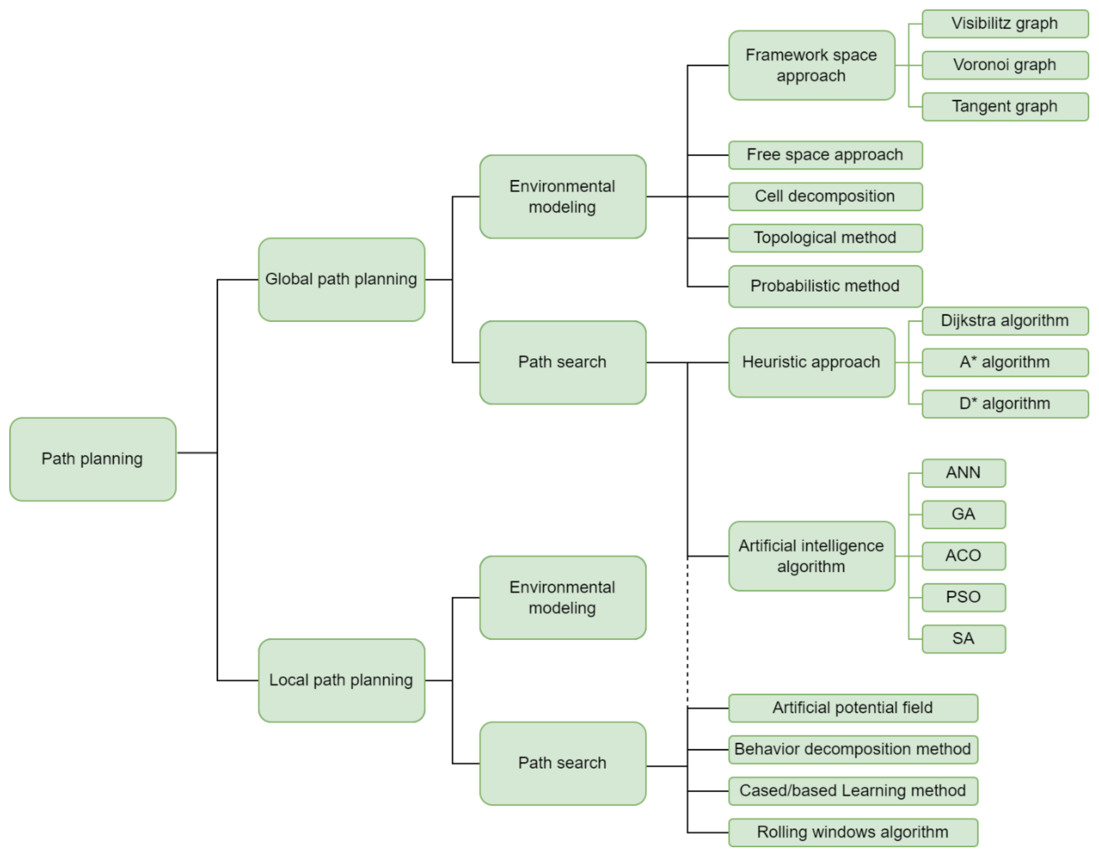
18], the author added a group of approaches called heuristic approaches compared to the previous author. He included artificial intelligence methods in this subset, such as neural network planning, fuzzy logic, genetic algorithms, and particle swarm optimization. As a result, he evaluated that heuristic methods are more suitable for dynamic environments. The author dealt with this area in a more complex way in [
19], where his view of this area is captured in
Figure 2. Here, the author mainly focused on global travel planning methods. His approach divided the environment modeling, optimization criteria, and path search method into three steps. The step, which he called the optimization criteria, can be considered as inserting inputs into the third step for optimal path search. He used methods such as the framework space approach, the free space approach, cellular decomposition, topological methods, and probabilistic road maps. He divided the search for a path into two areas, the heuristic and the field of artificial intelligence.
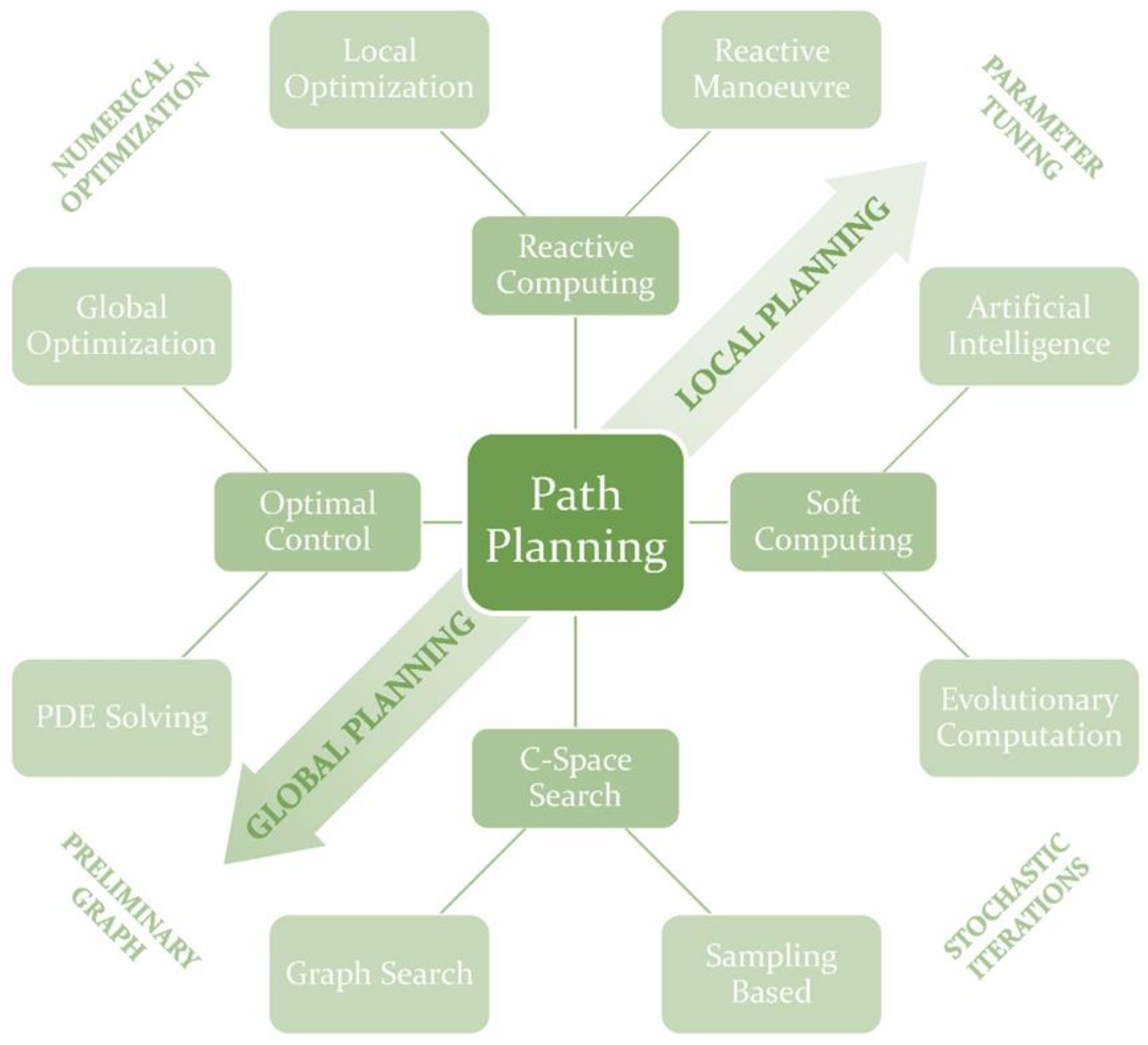
As we have noticed, in [
18,
19], there was a conflict in the division of methods under the designation heuristic. If we looked further in the area of categorization of this issue, we would find further discrepancies. Based on these discrepancies, the author in [
20] chose a different approach to solve this issue. He divided all the used methods into four areas, namely Reactive computing, Soft Computing, C-Space Search, and Optimal Control. This distribution can be seen in
Figure 3. In addition, each subcategory may have something in common with another subcategory.
We decide to use the A* algorithm to plan the route. Algorithm A* is used to search a discrete state space. The output should be the optimal trajectory from the initial state to the target state.
2.2. Representation of Space
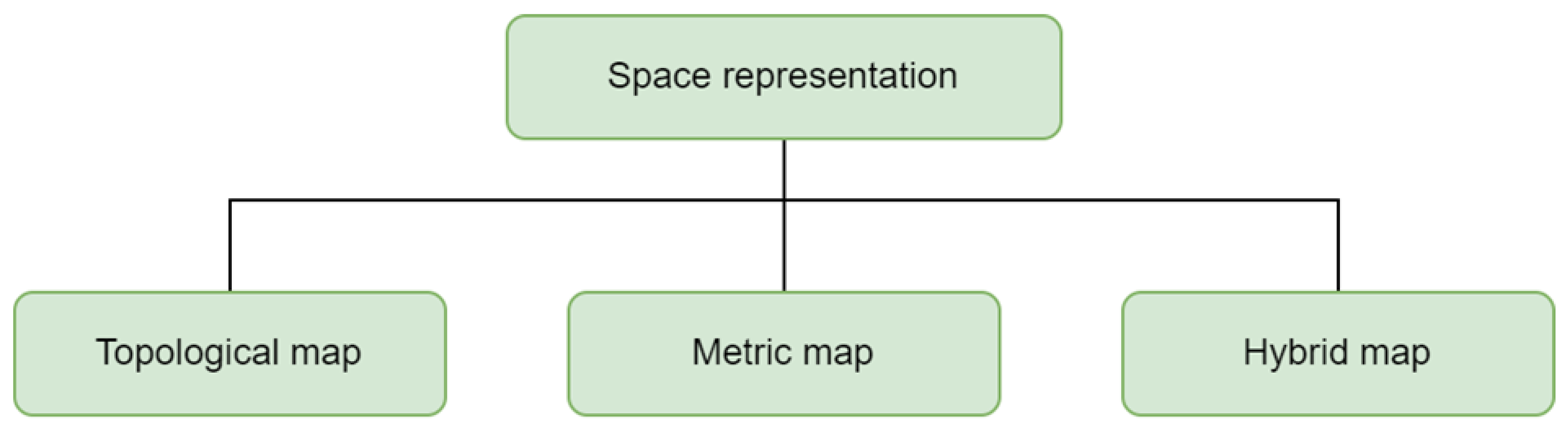
The space being described can be represented as continuous or discrete. In the real world, the environment is continuous, which complicates the solution in finding the optimal route, as continuous space is described by a set of infinite possible states. For simplicity, the continuous environment is divided into a finite set of states. This process is called environmental discretization. Finding a path then means searching for a sequence of states leading to the destination state. The state represents a point in space. The basic types of space representations can be divided according to [
21], into metric, topological, and hybrid, see
Figure 4. In each variant, localization in space is a basic problem, but of a different nature. The represented environment is often called the environment map. Based on what part of the environment the map represents, it is divided into a local or global map. They focus locally on the robot’s close surroundings, while global maps focus on the entire area. Metric maps represent objects in the environment based on their geometric properties. Two variants are most often used. The first is based on the calculation of Cartesian coordinates of the environment. Kalman filtration is often used here, using a fusion of odometric data and data from environmental sensors. The second variant takes the form of a grid map of occupancy. These maps are made from cells, which represent an estimate of the occupancy of individual cells in the environment [
21]. The way cells are divided and formed is dealt with by the cellular decomposition of the medium [
22]. The advantage of the metric map is the ability to create a detailed representation of the environment. However, higher demands on recording capacity and computing capacity are also related to this. However, the biggest disadvantage of this approach is that it does not provide a system for representing symbolic entities such as tables and doors. In a topological map, the environment is represented on the basis of its significant properties. This type of map takes the form of a graph, where nodes represent significant properties and edges represent relationships between properties. When creating a map, the uncertainty in determining the position of the mobile robotic system does not affect it. One of the problems with this approach is identifying the significant features and nodes in the environment that are used to create the map. The advantage of this map is considered to be fault tolerance in determining the position of the system in Cartesian coordinates, as it is not a priority when creating the map. A hybrid map is a combination of metric and topological, consisting of nodes and edges similar to a topological map. However, both edges and nodes can be described in the metric form of a map. This way of representing space uses the advantages of both mentioned forms. The metric description provides greater map detail, and the topological description increases resilience to localization errors. The problem arises when switching from one form of representation to another [
21].
The standard that deals with the data format for the needs of robotic system navigation, i.e., the map format, is called IEEE 1873–2015 [
23]. This standard defines the concept of a global map, which consists of local maps. A local map can consist of a metric map, a topological map, or a combination of both. In the context of the standard, grid maps and geometric maps are included in metric maps. A geometry map contains a list of contiguous geometric elements (such as points and lines). Topological maps already consist of the mentioned nodes and edges. Edges represent a direct (single jump) connection between adjacent nodes. In metric maps, the distance between two elements must be calculated, while in typological maps, this only applies to some elements. The output of the map defined by the IEEE 1873–2015 standard is in XML format. In our case, we decide to use grid map.
3. Design and Implementation
In this section, we focus in more detail on the procedure by which we try to identify dynamic objects in the mapped space. The whole procedure is summarized in Algorithm 1. The presumption for the functionality of the algorithm is available data in the form of 2D measurements and information about the position in which the measurement is performed. These input data are provided by the SLAM algorithm. The position estimate is written in the form of a matrix [x y θ], where x, y are the global coordinates of the measuring point and θ is the angle of rotation of the scanner. The first measurement is performed at coordinates [0 0 0]. The whole procedure is based on a comparison of three measurements, where
j is the measurement number.
| Algorithm 1 Dynamic Object Detection |
- Input:
Cell 2D environmental measurements, estimation of the position of each measurement - Output:
Clouds of points of dynamic objects, matrix of centers of dynamic objects
Transformation of measurements into a global coordinate system Creation of three consecutive point cloud measurements. Point cloud segmentation from j + 1 and j + 2 measurements Description of segment properties. Search for matching segments based on their properties. Creating a set of matching and nonmatching segments. Creating an area of interest based on the boundaries of each mismatched segment. Finding measurement points is an area of interest.
|
The used SLAM algorithm cannot directly generate global measurement coordinates; therefore, it is necessary to calculate them by estimating the measurement position. To recalculate the coordinates into the global system, we use relation, Equation (1), where
x′ and
y′ are the coordinates of the measurement position. The third coordinate is also needed to create a point cloud. This coordinate has a value of 0 for each measuring point.
After this step, we arrive at the data processing in the loop where scan matching is performed. At the beginning of the loop, three independent cloud points are created from three consecutive measurements ptCloudC(j), ptCloudA(j + 1), ptCloudB(j + 2). For ptCloudA and ptCloudB, segmentation and clustering of points based on Euclidean distance is applied. To compare individual clusters, it is necessary to define their properties, based on which they are compared. Here, a method is used to describe eigenvalue-based features. In this method, a vector consisting of seven values, (v)
→ = [linearity, planarity, scattering, omnivariance, anisotropy, eigenentropy, change in curvature], is created. The calculation of these values is made on the basis of the following relations, Equations (2)–(8).
The numbers
e1,
e2,
e3 are normalized eigenvalues that are defined on the basis of the relation
ei =
λi/∑
λ, where
i ϵ {1,2,3}. The variables
λ1,
λ2,
λ3, are nonnegative eigenvalues that correspond to the orthogonal system of eigenvectors. ∑
λ is given by Equation (9).
Assuming a point cloud formed by a total number of
N 3D points and a given value
k ∈
N, we may consider each individual 3D point
X = (
X,
Y,
Z)
T ∈
R3 and the respective k neighbors defining its scale. For describing the local 3D structure around X, the respective 3D covariance matrix also known as the 3D structure tensor S ∈
R3×3 is derived, which is a symmetric positive definite matrix. Thus, its three eigenvalues
λ1,
λ2,
λ3 ∈
R exist, are nonnegative, and correspond to an orthogonal system of eigenvectors. The author dealt with this issue in more detail in [
24].
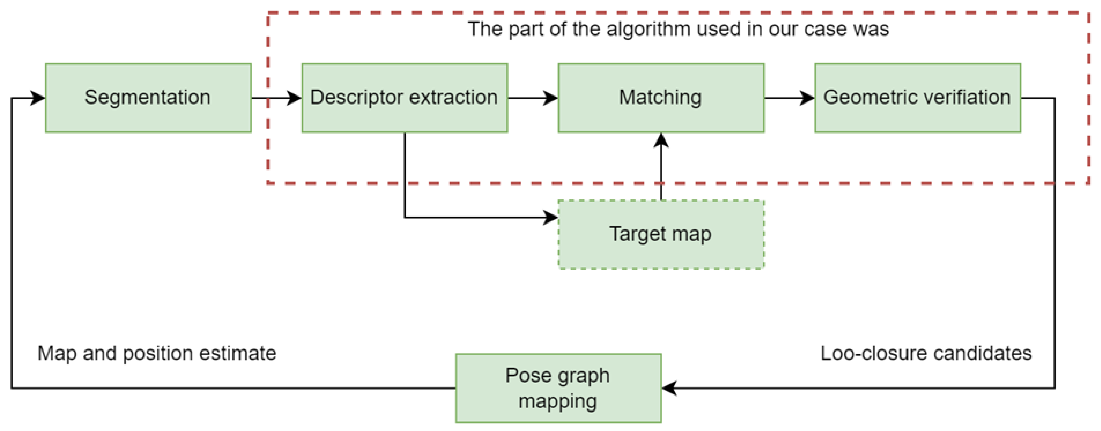
This whole process can be called function extraction. After assigning a property to each segment, you can move to the segment comparison technique. The segment recognition algorithm (SegMatch) is used for comparison. The comparison is performed between two point clouds (source and destination), which are divided into segments and have extracted segment functions. The SegMatch algorithm was designed for online real-time loop closure detection and localization. The principle of the functionality of the whole algorithm is shown in
Figure 5. From the whole algorithm, we use only the part that is marked in red in the figure. A more detailed description of the algorithm is discussed by the author in [
14,
25].
Properties from ptCloudA and ptCloudB are compared with each other. This comparison results in a set of matching and a set of mismatched elements. With matching elements, it is assumed that these are static elements of the map and they are no longer worked with. The set of mismatched elements from ptCloudB is processed as follows. Each cluster of points in this set is defined as a new point cloud. Its boundary
x and
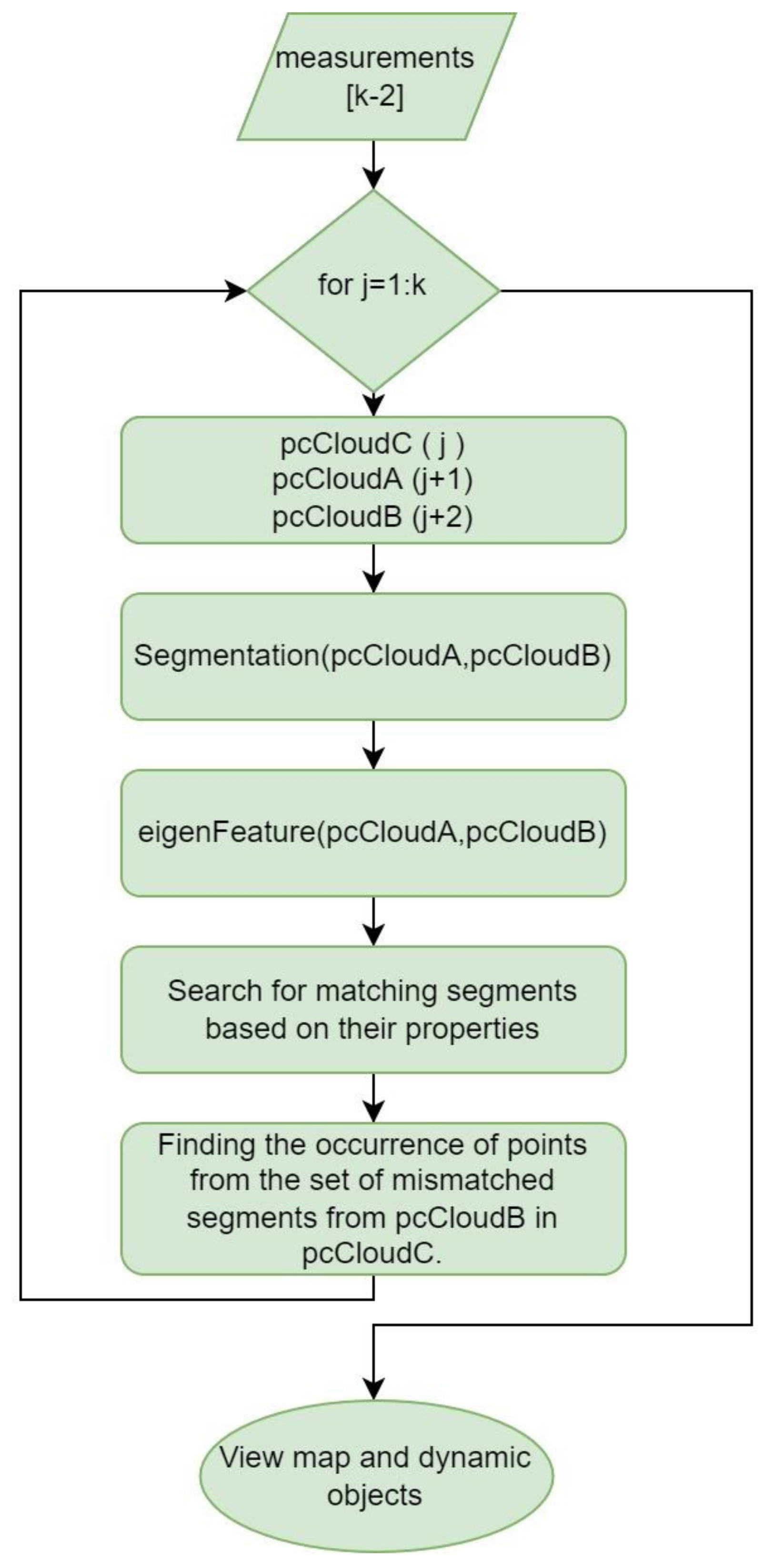
y coordinates are extracted from this cloud. Based on these coordinates, we obtain the area in which the potential dynamic object is located. In the last identification step, the occurrence of points in this area in ptCloudC is examined. If no match with ptCloudC is found, this cluster of points is considered a dynamic object. Each dynamically identified object is stored in a cell in the form of a point cloud. From each object, its geometric center is then calculated on the basis of formula (10). The whole mentioned procedure is summarized in
Figure 6.
3.1. Detection of a Dynamic Objects during Stationary Measurement
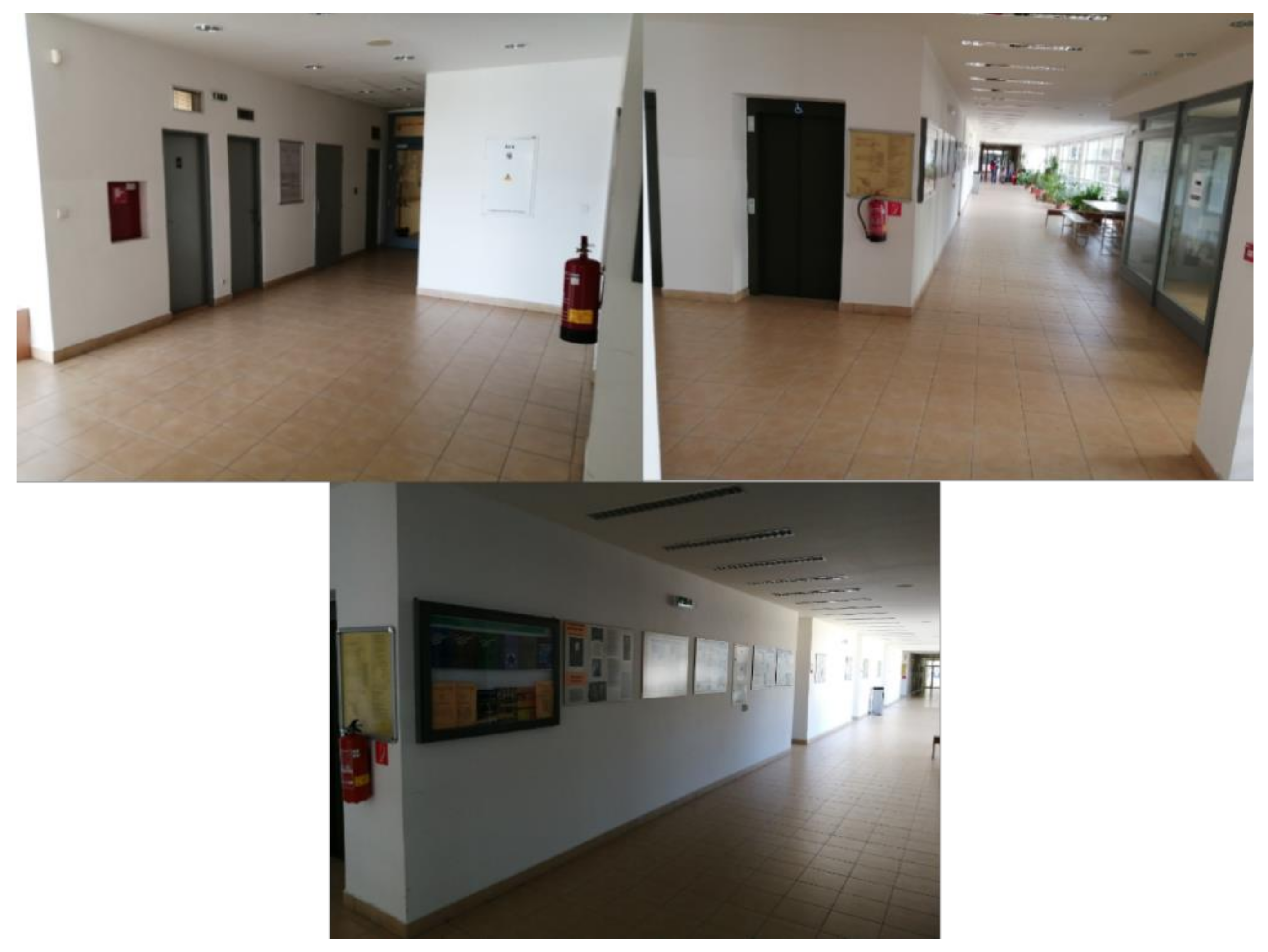
As a first step, we decided to test our proposed algorithm on a stationary measurement, in which the mapped environment was a dynamic object. The main goal was to determine how successful our proposed algorithm would work. The measurement took place in the corridors of our department. Photos of the environment can be seen in
Figure 7. This measurement also included objects that could cause noise in the measurement, such as glass doors and flowers, which we considered desirable, as the measurement did not take place in an ideal environment.
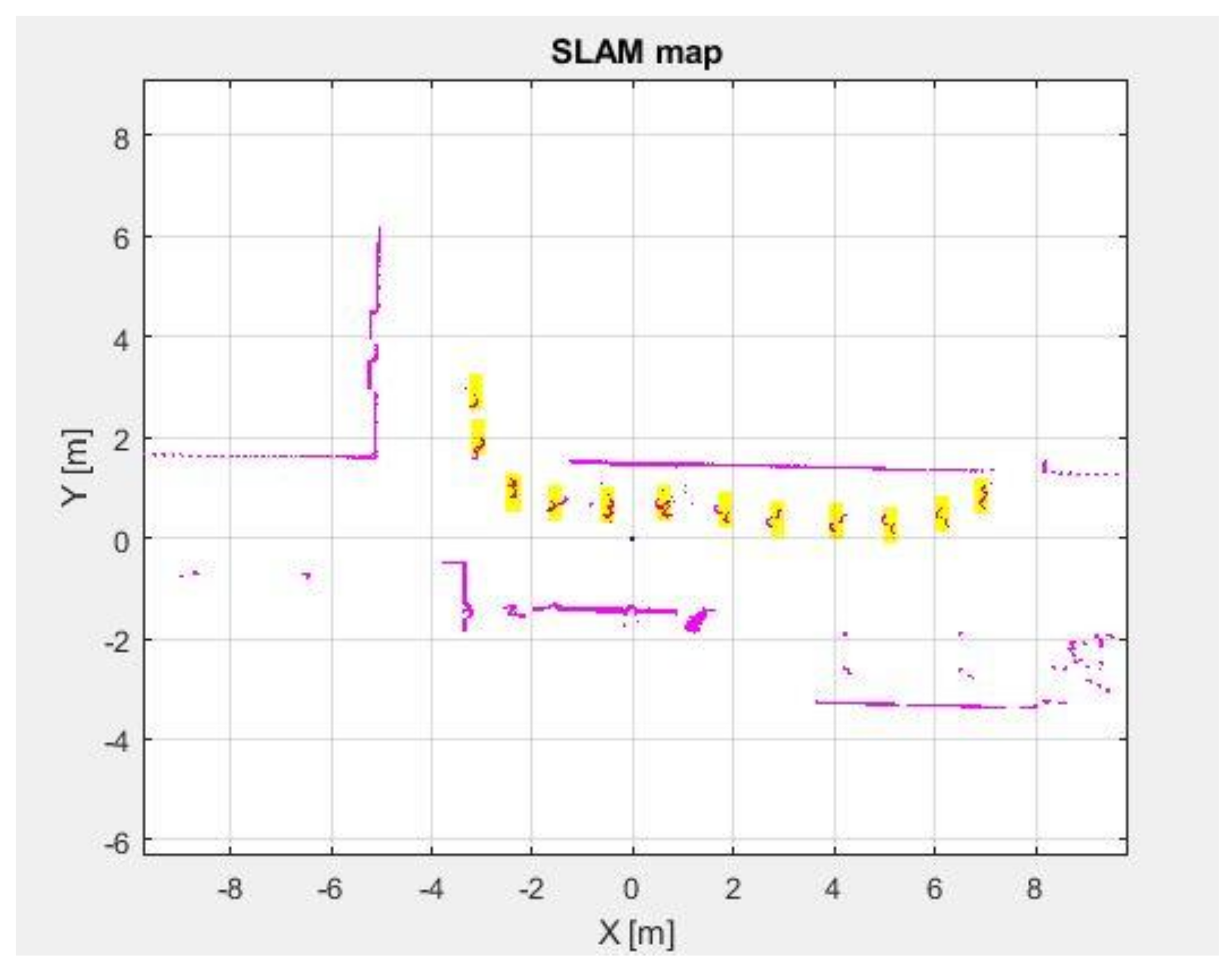
In the first step, data were collected from a lidar scanner. These data were entered into the SLAM algorithm in which the deviations were calculated and a 2D map was generated. This step was not necessary from the point of view of the whole measurement, as it was a stationary measurement and the position of the scanner did not change, but the output served as a visual check for the detection of dynamic objects. This map can be seen in
Figure 8. The dynamic object that we wanted to identify using the proposed methods is highlighted in yellow. The whole map consisted of 16 measurements, while the object of our interest was in it 12 times. The measurement was performed at point [0 0].
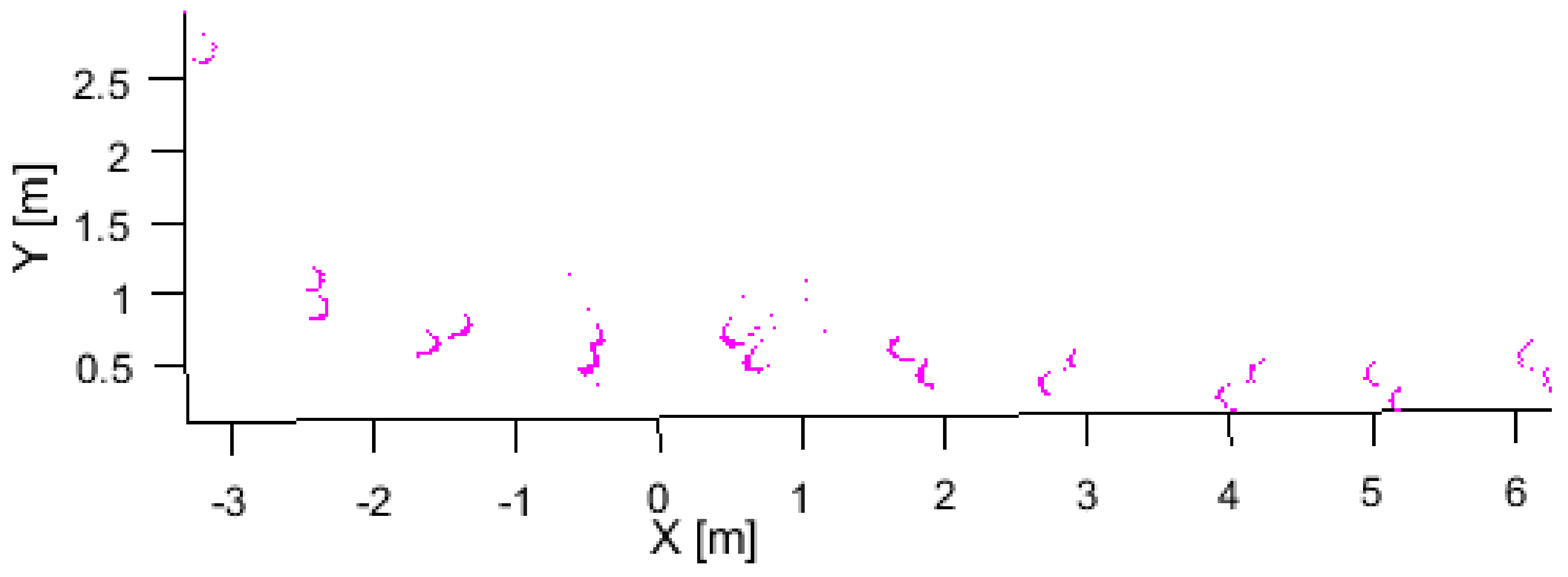
After generating the map, we processed the data into a suitable form for creating a point cloud. After editing the data, we applied the proposed algorithm to identify dynamic objects. As a result, the dynamic objects were displayed on a graph, which can be seen in
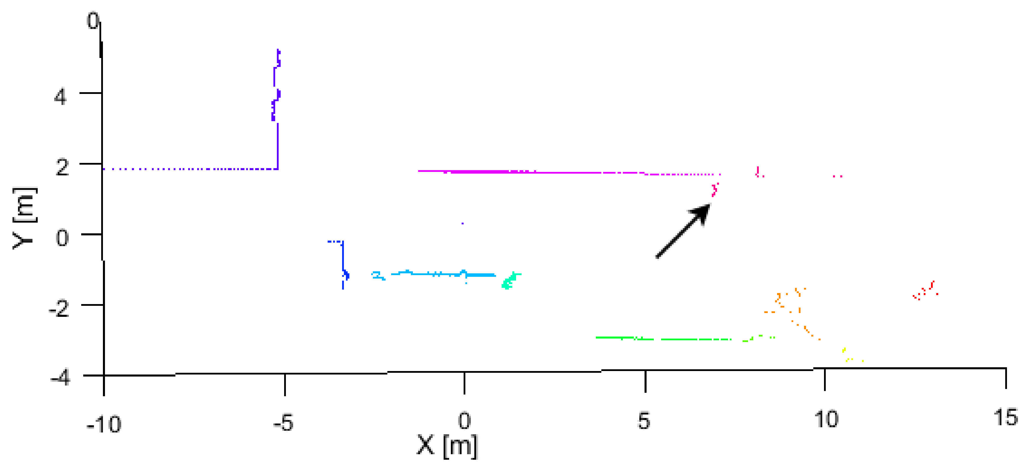
Figure 9. The number of identified dynamic objects was 11, which was one fewer compared to the original map. The problem with identifying an object was that the object was too close to the wall, which resulted in uniting the edge of the wall and the object when creating the segments. This problem can be seen in
Figure 10, where each segment is separated by a different color. An incorrectly segmented object is indicated by an arrow.
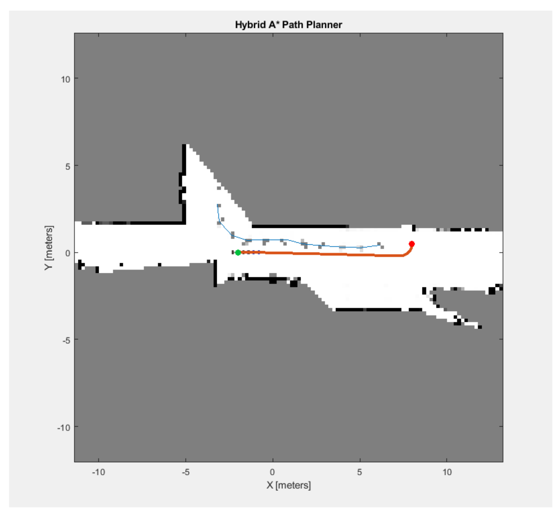
Once the dynamic object data were obtained, the data were edited and added to the data to create a navigation map. After creating this map, it was possible to apply navigation algorithms. The addition of a dynamic object to the navigation map was in order to take into account the trajectory of the dynamic object’s motion, in finding a suitable path. The application of the navigation algorithm can be seen in
Figure 11. The blue line represents the trajectory of the dynamic object and the red line symbolizes the route calculated using the A* algorithm. The time was recorded during the measurement, due to which we had the opportunity to determine the average speed of the object. In this case, it was 3.48 km/h.
3.2. Tests Performed during SLAM
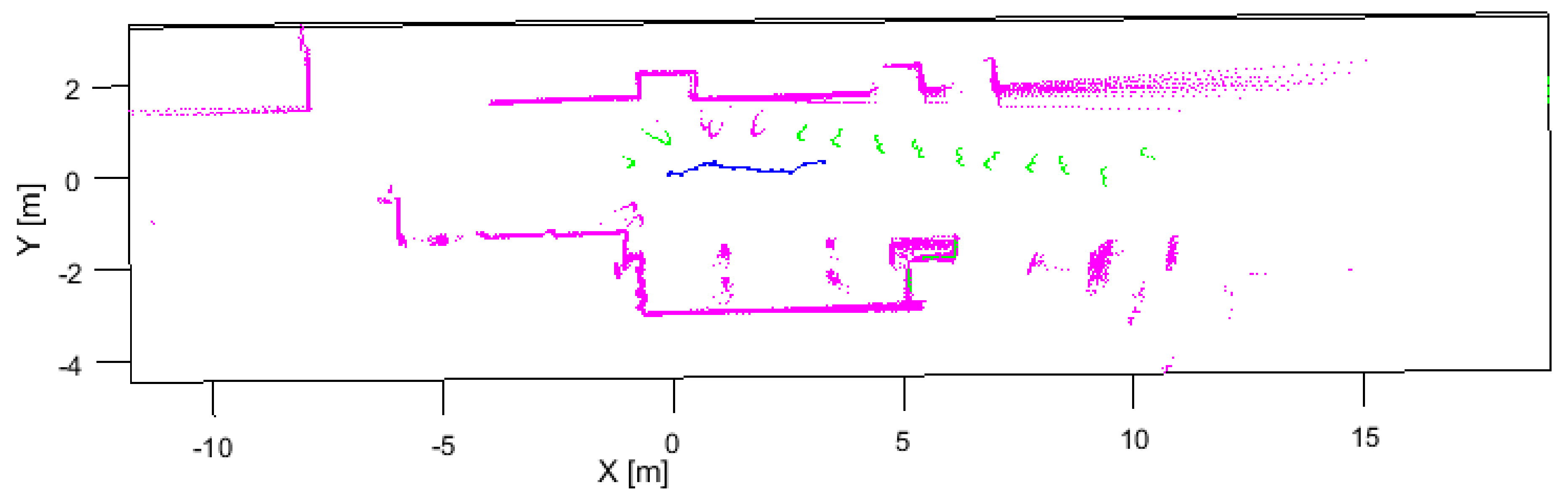
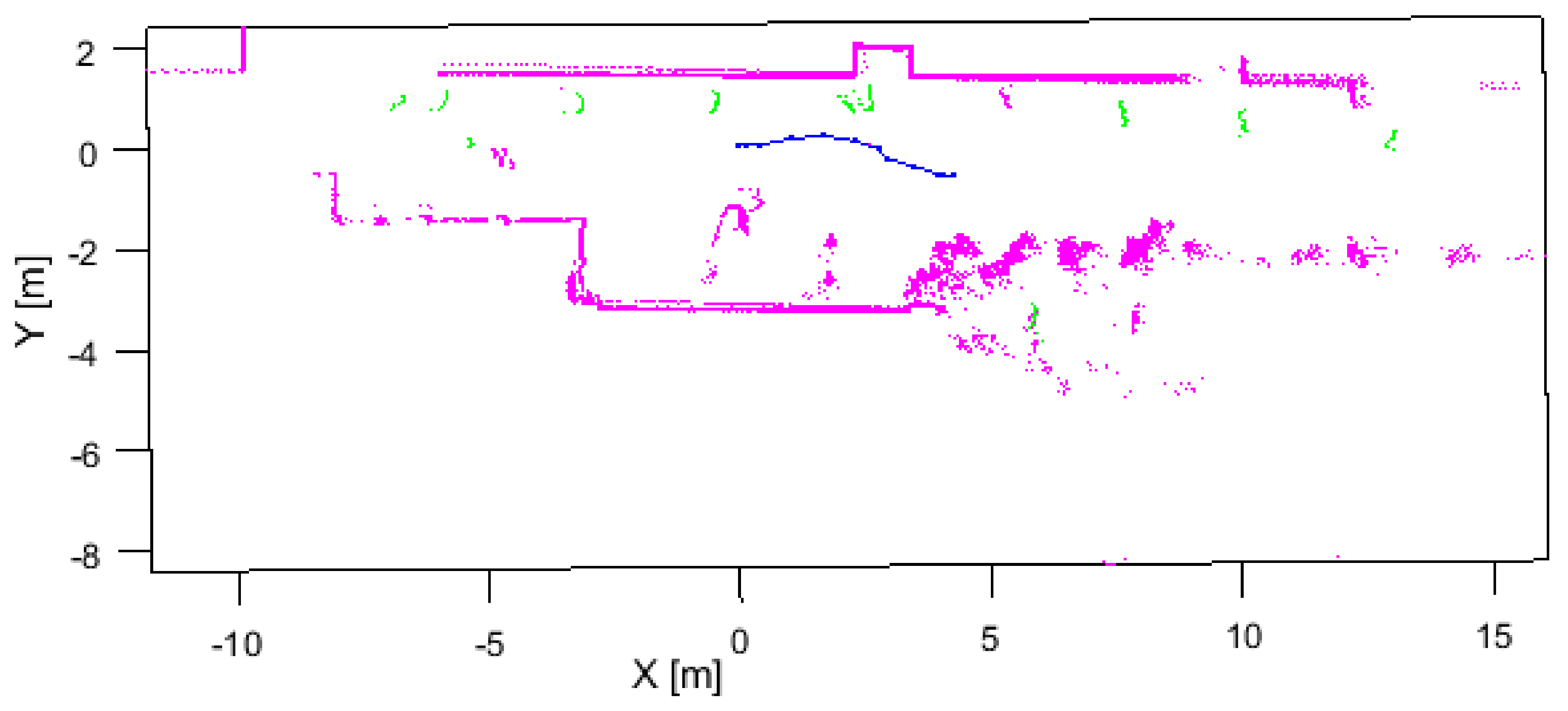
After testing on static measurements, we decided to use the proposed algorithm when performing SLAM. This was the last step before real-time testing. For the first test, 16 measurements were used with a sampling period averaging 1.2 s. During this measurement, the mapping device traveled approximately 3.3 m. A total of 15 objects were found during the identification of dynamic objects, 3 of which were falsely identified (walls), and 3 objects were not recognized, as they were assigned to a wall during segmentation and clustering. Dynamic objects are on the map in
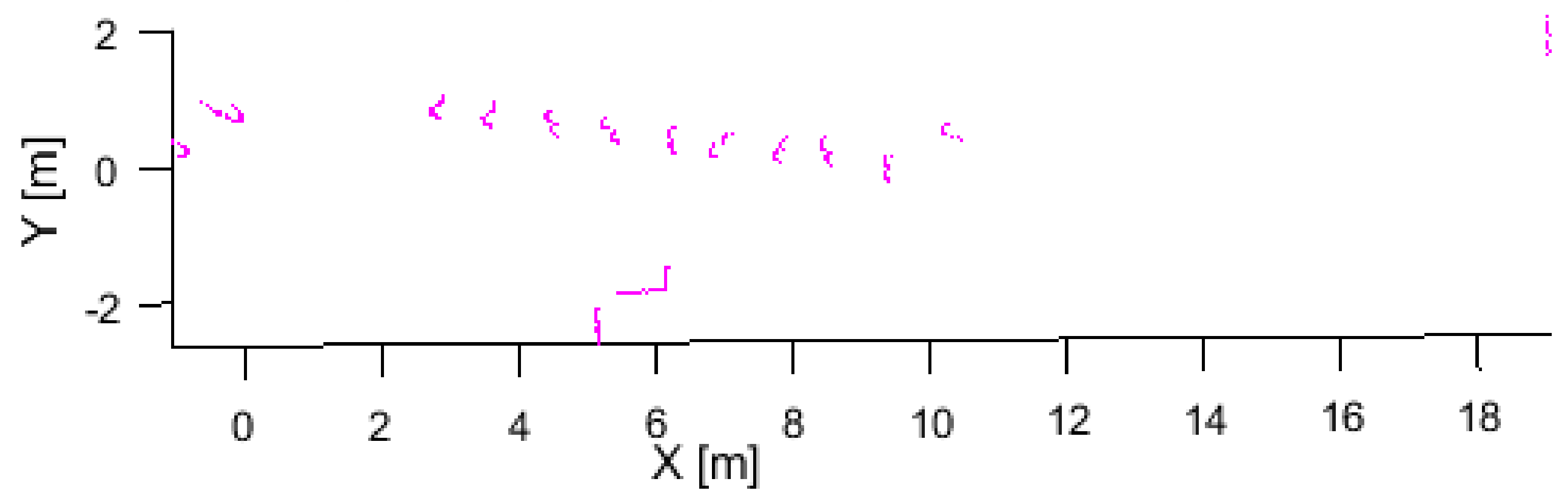
Figure 12 drawn in green, and blue indicates the trajectory of the measuring system. The total distance traveled by a dynamic object was approximately 11.7 m, while its average speed was 3.19 km/h. In
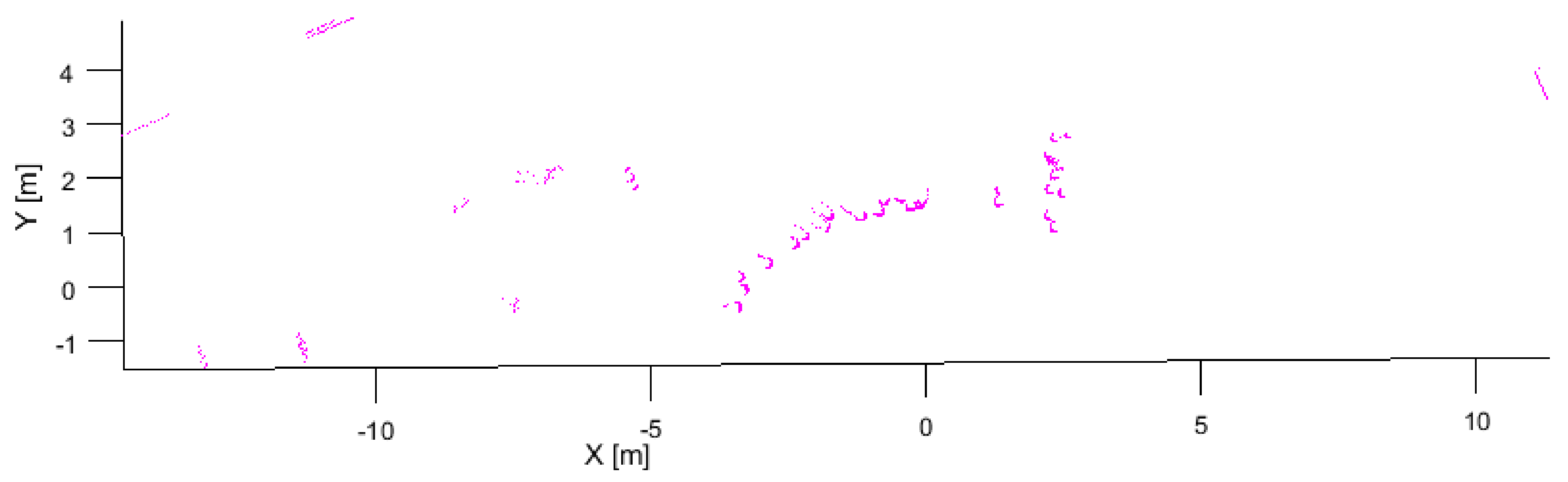
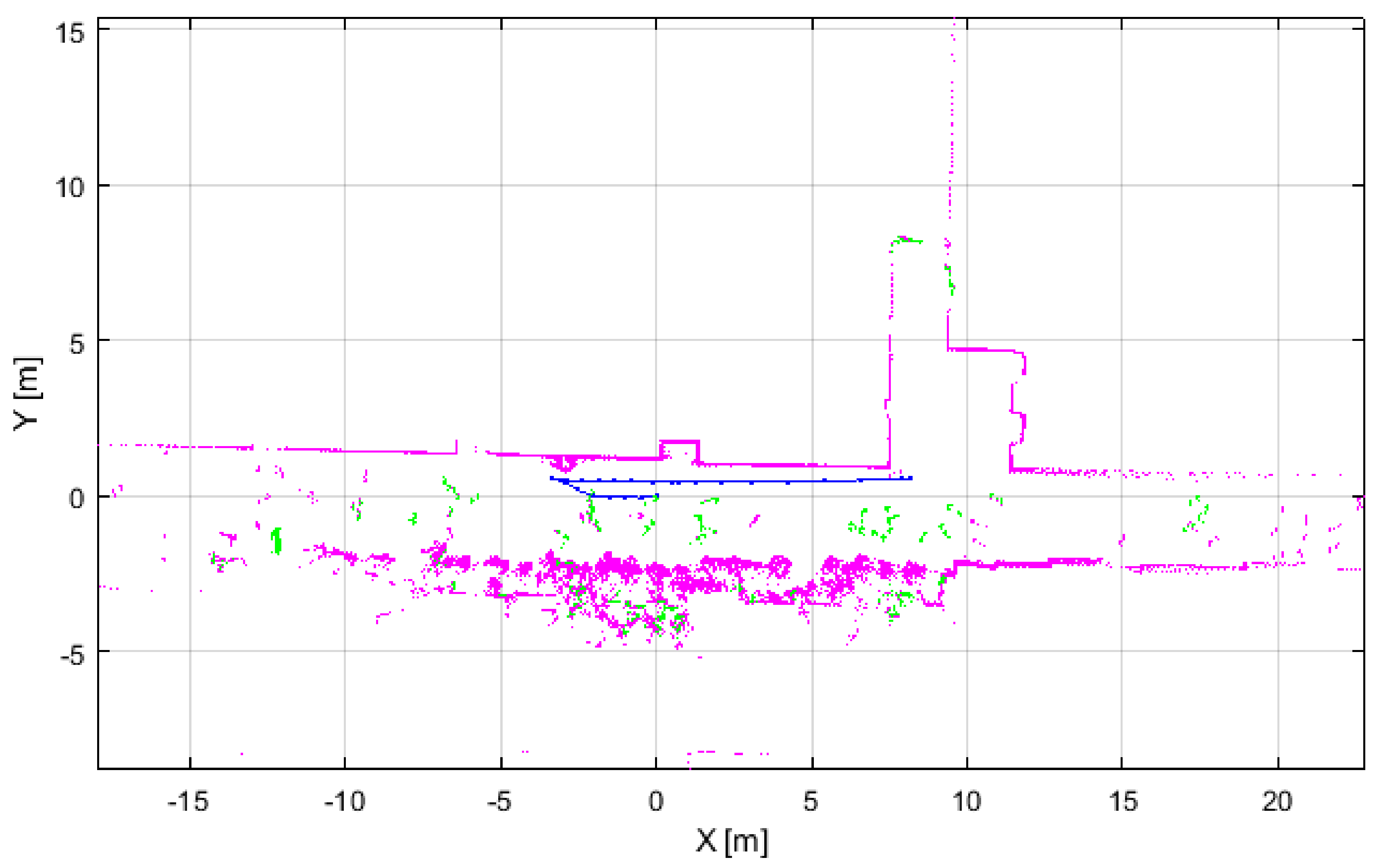
Figure 13, identified objects are plotted. One of the other measurements that were made was if the object was moving at a low speed when the sampling frequency was very high, and there would be a problem of overlapping measurements. The result can be seen in
Figure 14 and
Figure 15. A total of 25 measurements were used in this test. In this case, 29 objects were identified, of which 11 were falsely identified objects. There was a problem with the light reflectance as the sidewall in the corridor where the measurements took place was made of glass. In six images, the subject could not be recognized, due to the overlap of the subject area.
3.3. Real-Time Measurement
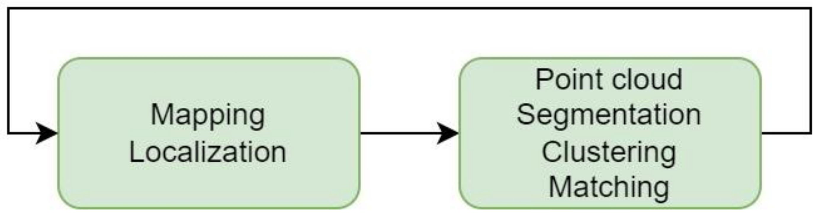
After the functionality of the proposed method was verified, we decided to perform mapping and identification of dynamic objects simultaneously. When testing such a case, the whole process was run in a loop, alternating part of SLAM and dynamic object identification. This procedure can be seen in
Figure 16. In the first step, it was necessary to process the measured data from the 2D lidar and locate it on the map. Based on the accuracy of this step, a further direction of the calculations took place. In the second step, the individual measurements were transformed into a point cloud. The point cloud was segmented and point clusters were formed. These clusters were then compared and the presence of a dynamic object was evaluated.
As already mentioned, the finding of dynamic objects is based on a comparison of three measurements. Therefore, at least three measurements are needed before the first comparison is made. After performing three initialization measurements, the identification of objects with mapping alternates regularly.
During the first measurement, we realized that the main limiting element would be the computing power of the evaluation unit. A laptop with 8 GB RAM and a 2.2 GHz dual-core processor was used for our measurements. A total of 13 measurements were made in this test. The execution of one cycle, which included SLAM and identification, took an average of 4.53 s. The identified dynamic object passed a 19 m track at a speed of 1.5 km/h. Our mapping device passed the 4.5 m track with a speed of 0.35 km/h. Again, the problem of glass reflectance and incorrect segmentation occurred during this measurement. The results can be seen in
Figure 17.
3.4. Applying Dynamic Object Detection While Moving to the Target Position
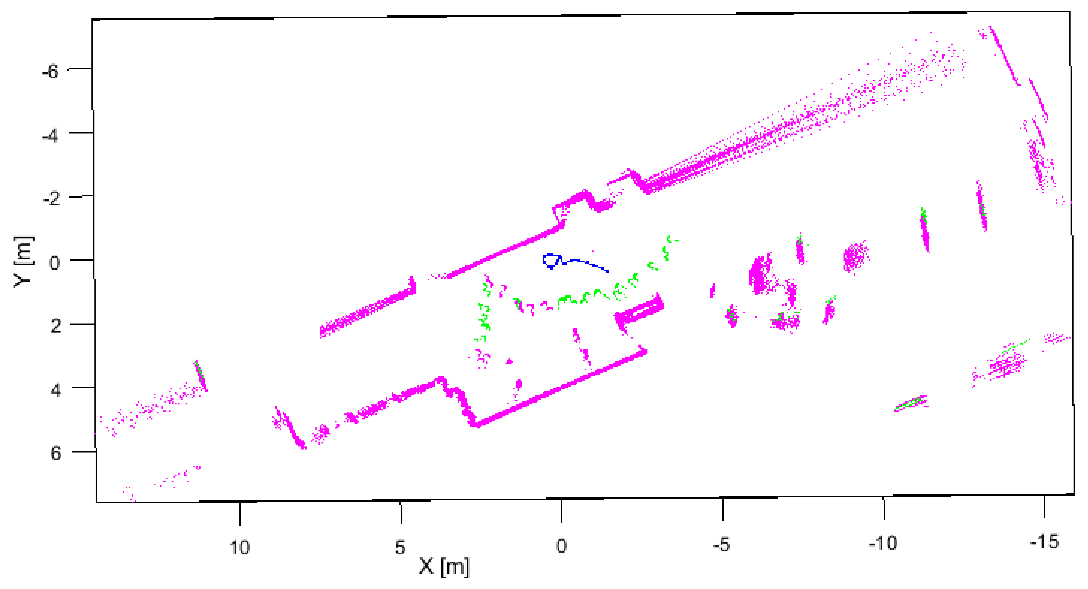
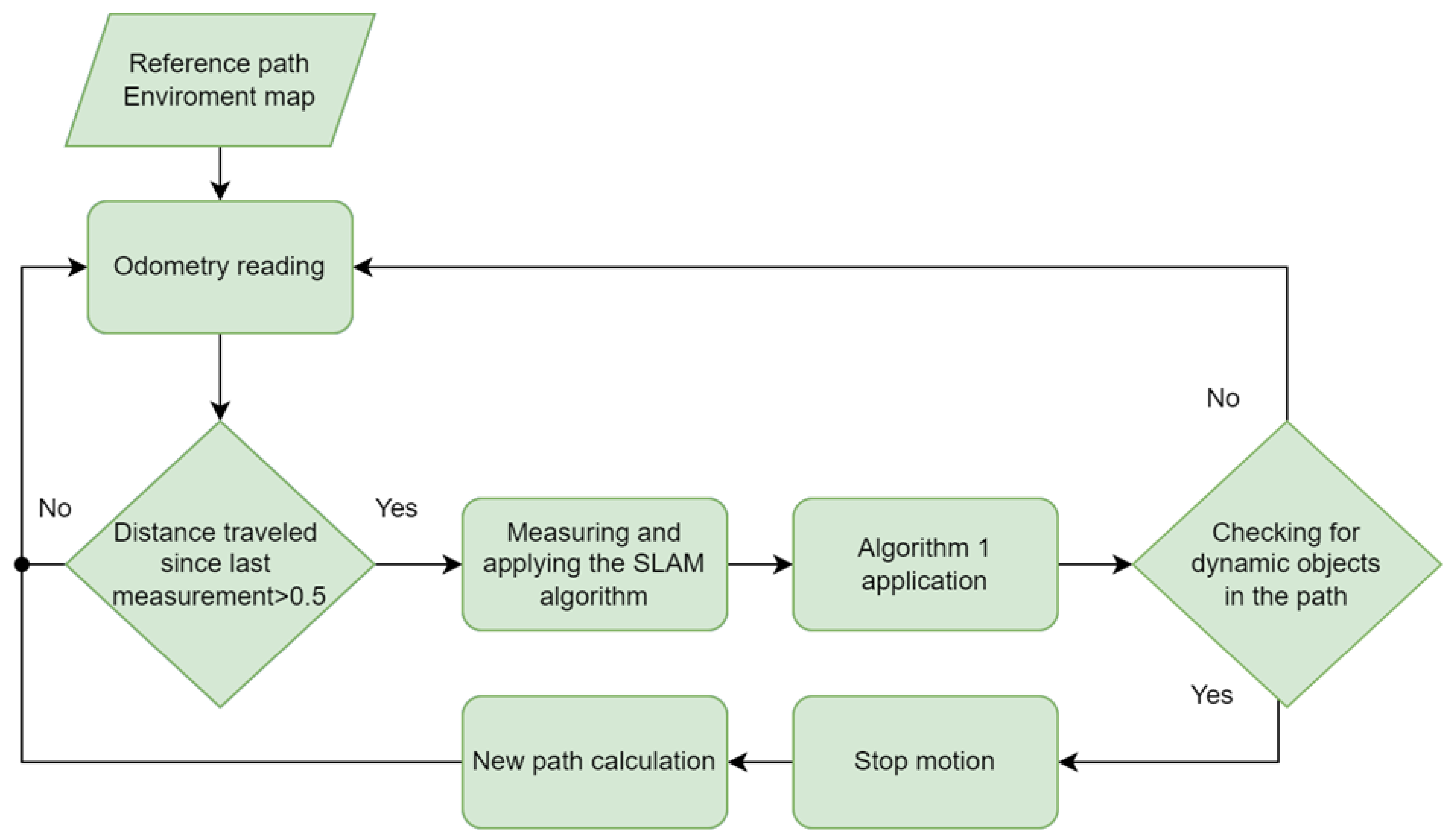
One of the other goals we set was to apply Algorithm 1 during the execution of active SLAM, in order to avoid dynamic objects during the execution of the movement to the target position. As the total detection time was about 4 s, optimization was necessary. During the optimization, some auxiliary processes were removed, which were used to visually check the functionality of the entire process. In addition, a more powerful computing unit was provided, which resulted in a faster process. As a result, the response time averaged 0.3 s where the value interval was <0.20;0.65>. After these results, it was possible to consider a reasonable time response of the whole system when detecting a dynamic object. Here, there was a need to properly place Algorithm 1 in an ongoing active SLAM. Detection of dynamic objects was implemented in the part where the robot was moving and reading its odometric data. The result of this implementation can be seen in
Figure 18, where a combination of ASLAM and object detection was used. Detected objects are marked in green on the map. The measurement was performed at a time when the corridor was quite busy.
After the successful implementation of Algorithm 1 during ASLAM execution, it was necessary to determine the extent to which the detection of dynamic objects would interfere with the activity performed during ASLAM. In this step, the conditions under which the robot would stop and calculate a new path had to be determined. As mentioned above, from each identified object, we obtained information about its geometric center in global coordinates using relation, Equation (11).
where
xmin and
xmax are the boundary coordinates of the object. Alternatively, the y coordinate is calculated. Based on these coordinates, the distance from the planned trajectory is calculated. If the object is located at a distance of 0.5 m from the planned trajectory, the robot is stopped and calculates the new trajectory. In order to determine the new trajectory, which means that the identified object is in the place where the robot has already passed, it is necessary to update the path that it still has to take, based on the measurement. The whole implementation process is shown in
Figure 19. It should be added here that this whole procedure was performed only when the robot was moving. One of the things to consider was the possibility of stopping the object at the robot’s target. In this case, the area around the destination was clear and a new navigation destination point was selected.


 ,
, 


