
A Spatial Fuzzy Co-Location Pattern Mining Method Based on Interval Type-2 Fuzzy Sets


School of Information Science and Engineering, Yunnan University, Kunming 650500, China
*
Author to whom correspondence should be addressed.
Appl. Sci. 2022, 12(12), 6259; https://0-doi-org.brum.beds.ac.uk/10.3390/app12126259
Submission received: 29 May 2022
/
Revised: 15 June 2022
/
Accepted: 16 June 2022
/
Published: 20 June 2022
(This article belongs to the Collection Geoinformatics and Data Mining in Earth Sciences)
Abstract
:The goal of spatial co-location pattern mining is to find subsets of spatial features whose instances are often neighbors in a geographical space. In many practical cases, instances of spatial features contain not only spatial location information but also attribute information. Although there have been several studies that use type-1 fuzzy membership functions to mine spatial fuzzy co-location patterns, there is great uncertainty associated with such membership functions. To address this problem, we propose a spatial fuzzy co-location pattern mining method based on interval type-2 fuzzy sets. First, we collect the interval evaluation values of the interval data of attribute information from experts to form granular data. Next, the original type-1 fuzzy membership function is extended to a granular type-2 fuzzy membership function based on elliptic curves. We use a gradual method to adjust the parameters of the fuzzy membership function so that its footprint of uncertainty satisfies both the connectivity and the given confidence. Based on this granular type-2 fuzzy membership function, we fuzzify the attribute information of instances and define the concepts of fuzzy features and fuzzy co-location patterns. A fuzzy co-location pattern mining algorithm based on spatial cliques is then proposed, termed the FCPM-Clique algorithm. In order to improve the efficiency of the algorithm, we propose two pruning strategies. In addition, we extend two classical spatial pattern mining algorithms, the Join-based algorithm and the Joinless algorithm, to mine fuzzy co-location patterns based on interval type-2 fuzzy sets. Many experiments on synthetic and real-world datasets are conducted, the performance of the three algorithms is compared, and the effectiveness and efficiency of our proposed FCPM-Clique algorithm is demonstrated.
1. Introduction
Spatial co-location pattern mining is an important branch of spatial data mining. A spatial co-location pattern is a subset of spatial features whose instances are often neighbors in space. For example, {hotel, restaurant} may be a prevalent co-location pattern because hotels and restaurants often neighbor each other in a city center. Spatial co-location pattern mining is widely used in the fields of botany [1], geographic information science [2,3,4], geology [5], urban facilities distribution, etc. For example, geologists may be interested in neighboring minerals in the same area [4].
In recent years, many algorithms for mining spatial co-location patterns have been developed. These algorithms can be divided into two types. Apriori-like algorithms [1,5,6,7,8] are one type. This algorithm first generates the candidate co-location patterns, then spends a lot of time generating row-instances of the candidate co-location patterns and checking their prevalence. Another algorithm is the algorithm based on prefix trees [2,3,9,10,11,12,13,14]. This algorithm generates maximal cliques from spatial datasets to discover prevalent spatial co-location patterns, which is generally more efficient than an Apriori-like algorithm. We have noticed that spatial data are often accompanied by attribute information expressed by specific values, such as the content of heavy metals in a certain geographical location [4]. However, existing spatial co-location pattern mining algorithms mainly focus on the location information of spatial data but ignore their attribute information.
In recent years, some researchers have used type-1 fuzzy sets to process the location information of spatial data and mine fuzzy co-location patterns (FCPs). However, type-1 fuzzy sets have a large amount of uncertainty. Type-2 fuzzy sets can model both intra-individual uncertainty and inter-individual uncertainty, while type-1 fuzzy sets can only model intra-individual uncertainty. Every expert can model a type-1 fuzzy set (intra-individual uncertainty), and the type-1 fuzzy sets of different experts are often different. Type-2 fuzzy sets can be used to fuse these different type-1 fuzzy sets, so as to consider the uncertainty between individuals.
In recent years, people have made great progress in the study of type-2 fuzzy sets [15,16,17,18,19,20]. Many researchers have applied fuzzy set theory to association rule mining. Anuradha et al. [21] used type-2 fuzzy sets to mine multi-level association rules. Lin et al. [22] used type-2 fuzzy sets to discover fuzzy frequent item sets efficiently. Kalia et al. [23] used type-2 fuzzy sets and genetic algorithms to mine fuzzy rules in high-dimensional classification tasks. Wang et al. [24] and Yang et al. [25] introduced fuzzy set theory into spatial co-location pattern mining and proposed a new metric method. Molina et al. [26] used a hierarchy to represent fuzzy association rules. Lin et al. [27] quickly discovered fuzzy frequent item sets from quantitative database based on type-2 fuzzy sets. Zhang et al. [28] mined the relationship between different types of crime rate based on fuzzy association rules. Wang et al. [29] and Anari et al. [30] combined a fuzzy set and rough set and proposed a new method of mining fuzzy association rules. In addition, fuzzy set theory is also widely used in attribute data mining. Gupta et al. [31] and Sun et al. [32] introduced fuzzy weight into fuzzy multi-attribute mining. Meng et al. [33] used interval type-2 fuzzy sets to solve multi-attribute decision-making in sponge city construction. Tao et al. [34] and Farhadinia et al. [35] applied ordered fuzzy sets to multi-attribute decision-making systems.
In recent years, many type-2 fuzzy membership functions have been proposed, such as ladder type, triangular type, Gaussian type and S type [36,37], π type [38], etc. However, these functions have a common feature: there are many parameters that determine the confidence and the width of the FOU, and the coupling between these parameters is very high, which makes it very difficult to select the appropriate parameters, for example, a type-2 fuzzy membership function based on an extended π function [38]. However, this is not the case for type-2 fuzzy membership functions based on elliptic curves [39,40] as there is only one parameter. Therefore, we generate an interval type-2 fuzzy membership function based on an elliptic curve.
We have noticed that spatial data are often accompanied by attribute information expressed by specific values, such as the content of heavy metals in a certain geographical location [4]. People are usually not sensitive to a specific value of the attribute information. However, when the attribute value changes fundamentally—that is, when it changes from a certain range to a new range—people will notice this and attach importance to the result. In this paper, in order to solve the large deviation caused by the method of mining fuzzy co-location patterns based on type-1 fuzzy sets [4], a method of mining fuzzy co-location patterns based on interval type-2 fuzzy sets and cliques from spatial datasets with attribute information is proposed.
The purpose of this paper is first to construct a special kind of interval type-2 fuzzy membership function—a granular type-2 fuzzy membership function based on interval type-2 fuzzy sets, which is used to improve the original type-1 fuzzy membership function. This reduces the deviation caused by the subjective evaluation of experts as far as possible, that is, to reduce the deviation caused by the uncertainty of a type-1 fuzzy membership function. Furthermore, we would like to find the influence of the uncertainty of fuzzy membership functions on the prevalence degree of fuzzy co-location patterns (FCPs) and measure the prevalence degree.
2. Innovation
Our paper makes the following contributions to the field of fuzzy co-location pattern mining:
- (1)
- In the fuzzy processing of corresponding attribute information based on the original type-1 fuzzy membership function, a granular type-2 fuzzy membership function based on an elliptic curve is generated from the evaluation data. We adopt a gradual method to adjust the parameters of the function so that the type-2 membership function not only meets the connectivity [11] but also makes its confidence reach the given threshold (set to 85%).
- (2)
- Based on the abovementioned granular type-2 fuzzy membership function, we define the concepts of fuzzy membership interval, upper bound participation ratio, lower bound participation ratio of fuzzy features, upper bound participation index, and lower bound participation index for FCP mining. Further, to smooth the “sharp boundary” of pattern prevalence and reduce the deviation caused by the subjective understanding of the prevalence degree of FCPs, we propose the concepts of absolutely prevalent FCPs, FCPs with a prevalence tendency degree, and absolutely non-prevalent FCPs.
- (3)
- Based on spatial cliques, a method of mining FCPs is proposed. First, an algorithm for generating spatial cliques from spatial datasets is presented, and then an Apriori-like algorithm and two pruning strategies are proposed to discover the absolutely prevalent FCPs and FCPs with a prevalence tendency degree. In addition, we apply interval type-2 fuzzy sets to traditional co-location pattern mining algorithms and form an FCPs mining method based on interval type-2 fuzzy sets and the traditional Join-based algorithm, as well as another FCPs mining algorithm based on interval type-2 fuzzy sets and the traditional Joinless algorithm.
3. Related Definitions and Theorems
3.1. Definitions
Traditional co-location patterns can reflect the spatial association of instances but ignore the influence of other information—besides location information—on the mining results. In order to articulate our method, we give the following definitions:
Definition 1 (Data fuzzification).
The most important step of attribute data fuzzification is to determine the fuzzy membership function. According to the fuzzy membership function, the attribute data is expressed as a fuzzy membership.
Supposing the fuzzy set over the domain is F, then the fuzzy membership function is . We use membership function to describe the fuzzy set F, that is, : x → [0, 1].
In this paper, we use the upper boundary and lower boundary of the footprint of uncertainty (FOU) to describe the type-2 fuzzy membership function. That is, we introduce the upper bound membership function (x) and the lower bound membership function F(x).
Definition 2 (Granular evaluation data).
We use the expert evaluation method to evaluate the interval membership degrees of the interval values under a fuzzy set to form granular evaluation data, so as to reduce the error when the specific membership degree of a specific value under a fuzzy set is evaluated.
Definition 3 (Fuzzy feature).
Fuzzy features refer to different types of things with fuzzy attributes in a space. A fuzzy feature set refers to the set of fuzzy features, expressed as Fuzz_Fea = {Fuzz_, Fuzz_, …, Fuzz_}. A fuzzy feature is represented as Fuzz_(1 i n).
The instances of a fuzzy feature are the sampling points of the fuzzy feature in the space and the fuzzy membership degree for the fuzzy feature when it is greater than 0.
Definition 4 (Neighborhood relationship).
A spatial dataset refers to the set of instances with type (feature), location information, and attribute information in a space. Suppose Fuzz_Fea is a set of features and S is the set of their instances, for any two instances, s1 and s2, if the Euclidean distance between the two instances is less than the threshold min_dist given by the user—that is, distance(s1, s2) ≤ min_dist—then the two instances satisfy the neighborhood relationship, which is represented as R(s1, s2).
Definition 5 (Fuzzy co-location pattern).
A fuzzy co-location pattern (FCP) Fuzz_c is a subset of the set of fuzzy features, that is, Fuzz_cFuzz_Fea. The size of an FCP is the number of fuzzy features of the pattern, which is expressed as |Fuzz_c|.
Definition 6 (Row-instance and table-instance).
Suppose there is a subset of spatial instances S ={s1, s2, …, sk} where any two instances are neighbors.If S contains all the fuzzy features of an FCP Fuzz_cand there is no subset of S that can contain all the fuzzy features of Fuzz_c, then S is called a row-instance of Fuzz_c. All row-instances of Fuzz_c constitute the table-instance of Fuzz_c.
Definition 7 (Absolute row-instance and absolute table-instance).
Suppose there is a spatial instance(i∈{1, 2, … k}). Ifis an instance of the fuzzy feature Fuzz_and also an instance of the fuzzy feature Fuzz_, thenis called an absolute row-instance of a fuzzy co-location pattern {Fuzz_, Fuzz_}. For a fuzzy co-location pattern, all its absolute row-instances constitute its absolute table-instance.
Definition 8 (Upper bound participation ratio and lower bound participation ratio).
Suppose there is an FCP Fuzz_c = {Fuzz_, Fuzz_, …, Fuzz_}, the lower bound participation ratio of the fuzzy feature Fuzz_(i∈{1, 2, … k}) is expressed as PR(Fuzz_c, Fuzz_), which is defined as the ratio of the sum of the lower bound membership degrees of the instances that appear non-repeatedly in the table-instance of the FCP Fuzz_c to the sum of the lower bound membership degrees of all the instances of Fuzz_. The upper participation ratio is expressed as(Fuzz_c, Fuzz_), which is defined as the ratio of the sum of the upper bound membership degrees of the instances that appear non-repeatedly in the table-instance of the FCP Fuzz_c to the sum of the upper bound membership degrees of all the instances of Fuzz_, namely:
Definition 9 (Upper bound participation index and lower bound participation index).
The upper bound participation index of FCP Fuzz_c is expressed as (Fuzz_c), which is defined as the minimum of the upper bound participation ratio of all fuzzy features Fuzz_ in Fuzz_c, which is:
The lower bound participation index of FCP Fuzz_c is expressed as PI(Fuzz_c), which is defined as the minimum of the lower bound participation ratio of all fuzzy features Fuzz_ in Fuzz_c, which is:
Definition 10 (Prevalent fuzzy co-location pattern).
According to Definition 9, an FCP Fuzz_c has an upper bound participation index and a lower bound participation index. For an FCP Fuzz_c when given a prevalence threshold min_prev, if (Fuzz_c)
< min_prev, Fuzz_c is called an absolutely non-prevalent pattern. If PI(Fuzz_c) ≥ min_prev, Fuzz_c is called an absolutely prevalent pattern. If PI(Fuzz_c) <min_prev (Fuzz_c), Fuzz_c is called an FCP with prevalence tendency degree, and the prevalence tendency degree of the fuzzy pattern is:
We call the absolutely prevalent FCPs and FCPs with a prevalence tendency degree prevalent FCPs.
Example 1.
We take the content of heavy metals, copper and zinc, in the topsoil of an area as an example. We divide the areas into the agricultural area (functional area A), residential area (functional area B), industrial area (functional area C), and commercial area (functional area D). Then, we sample the surface soil of each functional area and then measure the heavy metal content at each sampling point. The number of sampling points of functional areas, spatial location of sampling point, copper content, and zinc content are shown in Table 1. The spatial position of the sampling points are shown in Figure 1.
Suppose there is an FCP Fuzz_c = {A.Cu(M), B.Cu(H), C.Cu(M)}. Here, the fuzzy feature B.Cu(H) represents the B functional area with a high copper content. The size of the FCP is 3. According to the granular type-2 fuzzy membership function constructed in Section 4.1, we obtain the interval membership of the attributes of the instances in Table 1, as shown in Table 2. As can be seen from Table 2, the instances of fuzzy feature A.Cu(M) are A.1, A.2, and A.3; the instance of fuzzy feature B.Cu(H) is B.1; and the instance of fuzzy feature C.Cu(M) is C.1. If A.2, B.1, and C.1 are neighbors, {A.2, B.1, C.1} is a row-instance of the FCP Fuzz_c. According to Definition 8, the lower boundary participation ratio of these three fuzzy features is PR(Fuzz_c, A.Cu(M)) = 0.2256, PR(Fuzz_c, B.Cu(H)) = 1, PR(Fuzz_c, C.Cu(M)) = 1 and the upper bound participation ratio of these three fuzzy features are (Fuzz_c, A.Cu(M)) = 0.2866,(Fuzz_c, B.Cu(H)) = 1,(Fuzz_c, C.Cu(M)) = 1, so the lower participation index is PI(Fuzz_c) = 0.2256 and the upper bound participation index is (Fuzz_c) = 0.2866. If the prevalence threshold min_prev = 0.2, then PI(Fuzz_c) > min_prev, that is, Fuzz_c is absolutely prevalent. If the prevalence threshold min_prev = 0.3, then (Fuzz_c) < minprev and Fuzz_c is absolutely non-prevalent. If the prevalence threshold min_prev = 0.25, then (Fuzz_c) > minprev > PI(Fuzz_c) and the prevalence tendency degree θ of Fuzz_c is θ = 0.6.
3.2. Lemma and Theorem
Lemma 1.
The upper bound participation index (or lower bound participation index) of an FCP and the upper bound participation ratio (or lower bound participation ratio) of fuzzy features in a pattern decrease monotonically with the increase of the size of the pattern.
Proof.
If instance of fuzzy feature Fuzz_s is included in the row-instances of fuzzy pattern Fuzz_c, then when fuzzy pattern Fuzz_c’ Fuzz_c, instance Fuzz_c’ must also be included in the row-instances of Fuzz_c’. According to Definitions 8 and 9, the denominator of the upper bound participation ratio (or lower bound participation ratio) of the same fuzzy feature in the pattern and pattern Fuzz_c is the same, and the numerator decreases with the increase of the size of the pattern. Therefore, the upper bound participation ratio (or lower bound participation ratio) of the fuzzy features decreases monotonically. According to the definition of the upper bound participation index and lower bound participation index, the upper bound participation index (or lower bound participation index) is the minimum of the upper bound participation ratio (or lower bound participation ratio) of all fuzzy features in an FCP. Therefore, the upper bound participation index (or lower bound participation index) decreases monotonically with the increase of the size of the pattern. □
Theorem 1.
If a k-1 size pattern is absolutely non-prevalent, then any k size patterns that it contains are also absolutely non-prevalent.
Proof.
For a k-1 size pattern Fuzz_c, if a k size pattern Fuzz_c’ Fuzz_c, according to Lemma 1,(Fuzz_c’) ≤ (Fuzz_c). If this k-1 size pattern Fuzz_c is absolutely non-prevalent, then (Fuz_c) < min_prev. Therefore, if (Fuz_c’) ≤ (Fuz_c) < min_prev, then k size pattern Fuzz_c’ is also absolutely non-prevalent. □
4. Methods
4.1. A Mining Method Based on Spatial Cliques
We propose a method based on spatial cliques to mine all prevalent FCPs. Our method first uses a method based on a prefix tree to generate spatial cliques from spatial datasets; then an Apriori-like algorithm is used to generate candidate FCPs, find row-instances of candidates from the generated cliques, and then filter prevalent FCPs.
In this section, we discuss this approach in six subsections: generating granular type-2 fuzzy membership functions from type-1 fuzzy membership functions based on granular data (Section 4.1.1), materializing neighborhood relationships (Section 4.1.2), enumerating cliques (Section 4.1.3), generating candidate FCPs (Section 4.1.4), finding table-instances of candidates from cliques (Section 4.1.5), and filtering prevalent FCPs (Section 4.1.6).
4.1.1. Generating Granular Type-2 Fuzzy Membership Functions from Type-1 Fuzzy Membership Functions Based on Granular Data
When the specific membership degree of a specific value under a fuzzy set is evaluated, the deviation is often large. However, when the interval membership degree of an interval value in a fuzzy set is evaluated, the deviation can be greatly reduced. Therefore, we use the expert evaluation method to evaluate the interval membership degree of interval values under a fuzzy set to form granular data. Furthermore, according to the original type-1 fuzzy membership function, we generate a granular type-2 fuzzy membership function based on elliptic curves and gradually adjust the parameter of the granular type-2 fuzzy membership function by means of equal expansion.
- (1)
- Count the granular evaluation data.
In this process, we need to choose the appropriate length of the interval membership degree and the appropriate length of the evaluation interval data so that experts can make accurate judgments. We take the interval membership degree belonging to the fuzzy set Cu(M) as an example when the copper content is between 10 and 50. The interval length of the content we chose to evaluate is 5 and the length of interval membership is 0.1. If the length of the evaluated data is small, we set the interval length to 2—for example, when the copper content is between 6–20. We have counted the data of 1000 geologists who evaluated the interval value of copper content under the fuzzy set Cu.(M). The number in the particle indicates the number of evaluators who consider that an interval value corresponds to the interval membership. The darker the color is, the more people are evaluated in this interval. Figure 2a shows the number of evaluators of interval memberships.
- (2)
- The original type-1 fuzzy membership function is drawn based on the granular evaluation data.
In this example, according to the construction method in [4], we obtain the type-1 fuzzy membership function of heavy metal copper. We draw the type-1 fuzzy membership function, which is expressed as y = = , as shown in Figure 2b. Here, a is the lowest value that experts believe the heavy metal content tends to belong to the middle content, and b is the value that experts believe the copper content must belong to the middle content.
- (3)
- Constructing a type-2 membership function based on the original type-1 membership function.
The granular type-2 fuzzy membership function we proposed is represented by the upper bound fuzzy membership function and the lower bound fuzzy membership function. When the original type-1 membership function is a decreasing function, the formula is expressed as:
Upper bound function = .
Lower bound function = 1 − (a x b)
When the original type-1 membership function is an increasing function, the formula is expressed as:
Upper bound function =
Lower bound function = 1 − (a x b)
where a is the lowest value that experts start to believe has a tendency to belong to the fuzzy set and b is the value that experts believe must belong to the fuzzy set.
The area covered by the upper bound function and the lower bound function is expressed as the FOU. Here, determines the degree of expansion and contraction of the elliptic curve. The larger the value of , the larger the FOU; the smaller the value of , the smaller the FOU. In this example, when = 1.1, our granular type-2 fuzzy membership function is shown in Figure 3a.
A type-2 fuzzy membership function needs to satisfy two conditions: ① The FOU between the upper bound fuzzy membership function and the lower bound fuzzy membership function must be connected; and ② the proportion of data contained in the FOU to all data must reach a given threshold, that is, the confidence must reach a given threshold, which we set at 85% in this article. The granular data represents that, for any specific value in interval data, the possibility of taking any specific membership value in the interval membership is the same. Therefore, for interval data, the confidence of the type-2 membership function is . Here, n is the number of granules in the interval data, is the ratio of the area of the ith granule in the FOU to the area of the ith granule, and x are the number of evaluators in this granule. Within a range, the average of the confidence of all interval data is the confidence of the granular type-2 fuzzy membership function in this range.
- (4)
- Determine the parameters of the granular type-2 fuzzy membership function.
We use a gradual approach to determine the unique parameter in the granular type-2 fuzzy membership function. First, we set an increment α = 0.1, when = 1 + α ( = 1, 2, …, n). Then, we observe whether the FOU is continuous. If there is ψ (ψ {1, 2, …, n}) when = 1 + 𝜑α, the FOU is continuous; when = 1 + (ψ + 1)α, the FOU is not continuous. Then, set the gradual value to one-tenth of the original (i.e., β = 0.1α), = 1 + ψα + β ( {1, 2, …, 10}), and so on, until the accuracy reaches the user’s requirement and the FOU is connected. This process is shown in Table 3.
When = 1.283, the FOU of the granular type-2 fuzzy membership function is connected. At this time, the data in the FOU accounts for 85.13% of the total evaluation data, that is, the confidence of FOU is 0.8513, which reaches the default threshold. This is shown in Figure 3b.
The type-2 membership function we finally obtain from the granular data is shown in Figure 4 and Figure 5.
The upper bound membership function and the lower bound membership function of the granular type-2 fuzzy membership function are shown in Figure 4 and Figure 5. The values of of the granular type-2 fuzzy membership function of copper are 1.296, 1.283, 1.272, and 1.272, respectively. The values of of the granular type-2 fuzzy membership function of zinc are 1.28, 1.284, 1.284, and 1.272, respectively. The confidences of the granular type-2 fuzzy membership function of Cu are 0.8502, 0.8513, 0.8172, and 0.8953, respectively. The confidences of the granular type-2 fuzzy membership function of Zn are 0.8605, 0.8904, 0.8910, and 0.9022, respectively. The confidence of the granular type-2 fuzzy membership function in Figure 5c is 0.8172. If the confidence needs to be above 0.85, we can continue to select the appropriate step value and improve parameter by the gradual method.
- (5)
- Removing unconnected areas in the FOU.
After removing unconnected areas in the FOU, we can construct the segmented granular type-2 fuzzy membership function. Note that if the step value is too small, it may not reach the threshold, and if it is too large, it will lead to too many unconnected regions.
In this example, we set the step value as 0.1, then = 1.372, and the constructed type-2 fuzzy membership function is shown in Figure 6a. After removing the disconnected area, the piecewise function is shown in Figure 6b and the confidence is 0.8721, reaching the given threshold. In this case, the fuzzy membership function is expressed as:
From the above process, it can be seen that, based on the elliptic curve, the interval type-2 fuzzy membership function can be quickly constructed so that its FOU meets the connectivity and the confidence reaches the given threshold.
4.1.2. Generating FCP Mining Cliques (FCPM-Cliques)
According to the spatial neighborhood relation R, a spatial dataset can be expressed as a neighbor graph. We sort all of the features in the lexicographical order of their names. Instances of different features are sorted by their features, and instances of the same feature are sorted by their index values. We provide the following definitions:
Definition 11 (Small neighbor instance set).
For instance, s, with is the feature of instance s. A set of instances SN(s) = {s’|Fj < FiR(s, s’)} is defined as a small neighbor instance set of s, where Fj is the feature of s’. SNs(s) is a set of all the instances that are smaller than s and have spatial neighbor relationships with s.
Definition 12 (Big neighbor instance set).
For instance, s, with is the feature of instance s. A set of instances BN(s) = {s’| Fj > FiR(s, s’)} is defined as a big neighbor instance set of s, where Fj is the feature of s’. BNs(s) is a set of all the instances that are bigger than s and have spatial neighbor relationships with s.
In order to quickly find the neighborhood relationship among all instances, we use a method based on grids [6]. After finding the neighborhood relationship among all instances, we get the neighborhood table of all instances, as shown in Table 4.
Suppose there is a set of spatial instances S = {,,…,}, if there is {R(,) | 1 i k, 1 j k}, then S is a spatial clique—where a spatial clique is a fully connected subgraph in the instances distribution diagram. After obtaining the neighbor relationship between all the instances, we build a tree structure and adopt an effective method, called the Neighborhood Driven Method (NDM), to generate all spatial cliques.
For a spatial clique, the first instance of a clique is called the head of the clique and is represented by . ![Applsci 12 06259 i001]() . Last, all the cliques with instance as the head are represented by -clique. For example, for a clique = {A.1, B.2, C.2, D.3},
. Last, all the cliques with instance as the head are represented by -clique. For example, for a clique = {A.1, B.2, C.2, D.3}, ![Applsci 12 06259 i001]() = A.1,
= A.1, ![Applsci 12 06259 i001]() = {B.2, C.2, D.3}, is a -clique.
= {B.2, C.2, D.3}, is a -clique.
 . Last, all the cliques with instance as the head are represented by -clique. For example, for a clique = {A.1, B.2, C.2, D.3}, = A.1, = {B.2, C.2, D.3}, is a -clique.
After getting the neighborhood relation of all instances, the NDM aims to find these cliques headed by for each instance (1 i , where n is the total number of instances).
Definition 13 (NDM-Based clique tree (N-tree for short)).
An N-tree is a tree structure; its root node is labeled as “root”. In an N-tree, each node except “root” represents only one instance. Every branch of an N-tree is a spatial clique, which is called an N-clique. We use four strategies to construct an N-tree in the order of instances in the neighborhood table. Figure 7 shows an example of constructing an N-tree.
In a clique cli = {,,…,}, for any instance for of cli, {,,…,} is contained in BNs() and {,,…,} is contained in SNs(). Therefore, we check whether {,,…,} SNs(s)BNs() when we want to check whether an instance s and cli can form a new clique, which means that s is a neighbor to every instance in the clique and therefore a new clique can be formed. Four strategies are proposed according to the different situations of SNs(s)BNs().
Suppose there is a clique cli = {,,…,} and an instance s BNs().
Strategy 1: If the size of the clique |cli| = 1, SNs(s)BNs() = , s and cli can form a new clique because s BNs() and SNs(s).
Strategy 2: If the size of the clique |cli| > 1, SNs(s)BNs() {,,…,}, s and cli can form a new clique because cli and there is R(s,).
Strategy 3: If the size of the clique |cli| > 1, cli’ = SNs(s)BNs() {,,…,}, s and cli’ can form a new clique.
Strategy 4: If the size of the clique |cli| > 1, SNs(s)BNs(){,,…,} and {,,…,} SNs(s)BNs(), but cli’ = SNs(s)BNs() {,,…,}, s and cli’ can form a new clique.
The NDM uses four strategies to construct an N-tree in the order of instances in the neighborhood table. For instance s in the neighborhood table, we can get SNs(s). According to the four different situations of SNs(s) BNs(), we adopt four strategies to build the N-tree. After traversing each instance in the neighborhood table, an N-tree is completely established. The pseudocode for the NDM is as follows (Algorithm 1):
| Algorithm 1: Neighborhood Driven Method. |
| Input: nbsl: neighborhood relationship list (including SNs and BNs of each instance) S: a set of instances Output: list of N-cliques Steps: 1. nTree = Initialize N-tree; 2. For each instance s In nbsl.Instances Do 3. queue = SNs(s); 4. While NotEmpty(queue) Do 5. head = nTree.AddHeadNode(queue.Out); 6. bodies = GetCurrentBodies(head); 7. relation = queue∩BNs(head); 8. If bodies == null || relation == null Then 9. head.AddNode(s) 10. Else 11. For Each list l in bodies do 12. If l == relation Then 13. s and cli can form a new clique; 14. Else If relation ⊇ l Then 15. s and cli can form a new clique; 16. Else If relation ⊆ l Then 17. s and relation ∪s1 can form a new clique; 18. Else If NotEmpty(l ∩ relation) Then 19. s and relation ∩ l ∪s1 can form a new clique; 20. End If 21. End For 22. End If 23. End While 24. End For |
We use an example to illustrate the process of constructing an N-tree using the NDM. Figure 7 shows an example of constructing an N-tree according to the order of the instances in Table 4. In order to generate a clique with A.3 as its head (that is -clique), we start from A.3—there is BNs(A.3) = {B.3, B.4, C.1, D.1}. If we start from B.3, there is SNs(A.3) ∩ BNs(B.3) = , and, according to Strategy 1, A.3 and B.3 can form a clique. In the same way, there is SNs(A.3) ∩ BNs(B.4) = where A.3 and B.4 can form a clique. Then, SNs(A.3) ∩ BNs(C.1) = {B.3, B.4} according to Strategy 2, C.1 and {A.3, B.3} can form a new clique and C.1 and {A.3, B.4} can also form a new clique. Finally, SNs(A.3) ∩ BNs(D.1) = {B.4, C.1} according to Strategy 3, D.1 and {A.3, B.4, C.1} can form a new clique.
Definition 14 (Complete clique set).
Given a set of cliques scl of a spatial dataset materialized by spatial neighborhood relationships and the set containing all cliques of the spatial dataset is represented as ascl, if the following formula is satisfied, scl is a set of complete cliques:
∀ cl ∈ ascl, ∃ cl’ ∈ scl ⇒ cl ∈ cl’.
Lemma 3.
N-cliques are complete.
Proof.
Given a clique cl = {, , …, } where is an instance, if cl is a maximal clique, ∀s cl, s, and cl cannot form a new clique. It is not difficult to see that the NDM can generate all the maximal cliques. According to Definition 14, the set containing all maximal cliques is complete. Thus, N-cliques are complete. □
The four strategies (Strategy 1–Strategy 4) can make decisions concerning which node can be added to a clique to form a new N-clique, and, according to Lemma 3, we know that N-cliques are complete. Therefore, the cliques generated by the NDM are correct and complete.
In the process of mining spatial co-location patterns, we calculate the participation ratio of features according to the number of instances in a spatial clique. However, in the process of mining fuzzy spatial co-location patterns, we calculate the participation ratio of fuzzy features according to the membership degree of the attributes of instances in a spatial clique. Therefore, we pay more attention to the association between attributes of instances in the spatial clique, and we propose a kind of FCPM-clique and make the following definition: In a spatial clique, if there is an association between fuzzy attributes of instances, the fuzzy attributes of these instances can form FCPM-cliques.
We find that, in a clique, there is an association between fuzzy attributes of different instances, so they can form FCPM-cliques. There is also an association between fuzzy attributes with different attributes in an instance, so these can also form FCPM-cliques.
For example, for two neighbor instances A.1 and B.1, the fuzzy attribute Cu(M) of A.1 and the fuzzy attribute Cu(H) of B.1 can form an FCPM-clique {A.1.Cu (M), B.1.Cu (H)}, which can be used as a row-instance of FCP {A.Cu(M), B.Cu (H)}—as shown in Figure 8. For instance A.2, its fuzzy attributes Cu (H) and Zn (H) can form an FCPM-clique {A.2.Cu (H), A.2.Zn (H)}, which can be used as a row-instance of FCP {A.Cu(H), A.Zn (H)}—as shown in Figure 9.
For a candidate FCP, first we find the co-location pattern consisting of all the non-recurring features in the fuzzy candidate pattern. Then, we find the row-instances that contain all the fuzzy features of the fuzzy candidate pattern from the table-instance of the co-location pattern. These row-instances are the row-instances of the candidate fuzzy pattern. Through the FCPM-clique, we can find these spatial cliques containing all fuzzy features of the candidate FCPs.
4.1.3. Generating Candidate FCPs
In the process of generating candidate FCPs, we find that two fuzzy features with different features can form a candidate FCP; two fuzzy features with the same feature and different attributes can also form a candidate FCP. However, the FCP composed of fuzzy features with the same features and the same attributes has no practical significance, such as {A.Cu(L), A.Cu(M), A.Cu(H)}. In order to avoid producing such a meaningless candidate FCP, we propose an Apriori-like algorithm and bucket to generate complete candidate FCPs. The steps of the algorithm (Algorithm 2) are as follows:
| Algorithm 2: The algorithm for generating candidate FCPs based on buckets. |
| Input:} } (3) Instance set of fuzzy features S = {s1, s2,…, sn} (4) Spatial proximity relation R (5) Minimum distance threshold min_dist (6) Minimum prevalence threshold min_prev Output:: k + 1 size candidate FCPs Step: 1.if (k == 1) 2. for each Fuzz_f in Fuzz_Fea do 3. SetId(Fuzz_f) 4. Initialize_bucket(Fuzz_f) 5.else if (k == 2) 6. for each Fuzz_f_1 in one feature 7. for each Fuzz_f_2 in other feature 8. Generate a candidate pattern from Fuzz_f_1 and Fuzz_f_2 9. for each Fea in Fea_List 10. for each Fuzz_f_1 in the first attribute 11. for each Fuzz_f_2 in the second attribute 12. Generate a candidate pattern from Fuzz_f_1 and Fuzz_f_2 13. Put fuzzy patterns with the same features and the same attributes into the same bucket 14.else 15. for(i = 1; i < bucket_count; i++) 16. for each fuzzy pattern in bucket[i] 17. for(j = i + 1; j < bucket_count; j++) 18. for each fuzzy pattern in bucket[j] 19. if the first k – 1 fuzzy features of the two k-size fuzzy patterns are the same 20. Generate a fuzzy pattern ck+1 21. if (check(k − 1, ck+1, bucket)) 22. ck+1 is a new candidate fuzzy pattern 23. Put fuzzy patterns with the same features and the same attributes into the same bucket |
Steps 2–4: we put all fuzzy features with the same feature and the same attribute into the same bucket. Steps 6–8: size-2 candidate FCPs are generated by connecting the fuzzy features contained in any two different features. Steps 9–12: since the number of attributes is 2, all fuzzy features contained in a feature can be divided into two sets of fuzzy features with the same features and different attributes by connecting any two fuzzy features in the two sets of fuzzy features, and a size-2 candidate FCP is generated. Step 13: put the fuzzy patterns with the same features and the same attributes into the same bucket. Steps 15–22: generate k + 1 size candidates from k size prevalent fuzzy patterns; for any two prevalent fuzzy patterns, check whether the first k − 1 fuzzy features of the two fuzzy patterns are the same, and if they are same, connect them to generate a k + 1 size candidate fuzzy pattern. Finally, we check whether each sub-pattern of the newly generated k + 1 size candidate fuzzy pattern is prevalent. Step 23: put the fuzzy patterns with the same features and the same attributes into the same bucket.
4.1.4. Find the Row-Instances of the Candidate FCPs by the Column-Filter Method
In order to improve the efficiency of finding row-instances of candidate FCPs, we propose a column-filter method to find the row-instances of the candidate FCPs from the row-instances of co-location patterns. First, we find the co-location pattern consisting of all the non-recurring features in the candidate FCP. Suppose the number of fuzzy features contained in the FCP is n, we obtain the row-instance of the FCP through filtering n times. In the first filtering, for all row-instances of the co-location pattern, we filter all row-instances with the first fuzzy feature. In the second filtering, for the row-instances obtained by the first filtering, we filter the row-instances with the second fuzzy feature, and so on. In the nth filtering, for the row-instances obtained by the nth filtering, we filter the row-instances with the nth fuzzy feature. The row-instances obtained by the nth filtering have all the fuzzy features of the FCP, so these are the row-instances of the FCP.
For the fuzzy features contained in each feature, we calculate the ratio of the number of instances with the fuzzy feature to the number of instances with the feature, that is, = , = , …, = . Thus, for a fuzzy feature Fuzz_, it has a weight . Then, we sort the fuzzy features of the candidate FCP in order according to the value of from smallest to largest. Through the method, in the table-instance of the co-location pattern, the pruning rate of pruning the row-instances without the first fuzzy feature is the highest in the first filter. This greatly reduces the number of row-instances that need to be filtered in the second filter, and so on, until the row-instances that contain all the fuzzy features of the candidate FCP are filtered. In this way, we can greatly reduce the time cost to judge these row-instances and the efficiency is improved to a great extent. The pseudocode of this algorithm (Algorithm 3) is as follows:
| Algorithm 3: The column-filter method. |
| Input: } Table-instance Table_c of co-location pattern that contains the candidate FCP Output: Table-instances of candidate FCP Table[n] Step: 1. Table = Table_c; in the candidate FCP Fuzz_c 3. for each row-instance in Table 4. if (the row-instance doesn’t contain Fuzz_f_i) 5. Table.Delete(the row-instance); 6. end for 7. Table[i] = Table; 8. end for 9. if i == n 10. Table[i] is the table-instance of the candidate FCP |
Step 1: The filtering operation begins with Table_c, a table-instance of the co-location pattern that consists of the features of the candidate FCP. Steps 2–8: For all row-instances of the table-instance in Table_c, we judge whether they have the first fuzzy feature of the candidate FCP. For any one of the row-instances, if it does not have the first fuzzy feature, we delete it; in this way, we filter out all the row-instances with the first fuzzy feature. Then, we judge whether these row-instances have the second fuzzy feature and filter out the row-instances that have both the first fuzzy feature and the second fuzzy feature, and so on. Steps 9–10: If the selected row-instance has all the fuzzy features of the candidate FCP, then the row-instance is a row-instance of the candidate FCP and all row-instances of the candidate FCP make up its table-instance.
We compare the number of judgment operations between the column-filter method proposed in this section and the row-filter method proposed in Section 5.1 on average. For a candidate FCP of size p, assume that the number of row-instances of the co-location pattern composed of its features is q.
According to the row-filter method in Section 5.1, for each row-instance, we need to judge whether each instance has corresponding fuzzy features in turn. When there is at least one instance in a row-instance that does not have corresponding fuzzy features, the row-instance cannot be used as a row-instance of the candidate fuzzy co-location pattern. On average, each instance in a row-instance has the same probability of not having corresponding fuzzy features, so the expected number of judgment operations of a row-instance is = = . We need to judge each row-instance in turn, so the expectation of the total number of judgment operations is .
According to the column-filter method in this section, we set the number of fuzzy sets to three. In the average case, each fuzzy set contains the same number of instances, and each filtering operation can filter of the row-instances. Therefore, the expectation of the number of judgment operations of the column-filter method is q + + + … + = . When q is a constant value and p is large, < . Therefore, the column-filter method is more efficient than the row-filter method.
4.1.5. Filtering Prevalent FCPs
For a candidate FCP, after obtaining all its row-instances (these row-instances make up its table-instance) according to Definitions 8 and 9, we can calculate the upper bound participation index and lower bound participation index of the FCP. Then, according to the upper bound participation index, the lower bound participation index, and the prevalence threshold, we can filter prevalent FCPs. Therefore, we propose two pruning strategies to filter complete and correct prevalent FCPs from candidate FCPs.
Pruning strategy 1 (Fuzzy feature pruning):
In a candidate FCP, for any of its fuzzy features Fuzz_, if the upper bound participation ratio of the fuzzy feature is less than the given prevalence threshold min_prev, the candidate fuzzy pattern is absolutely non-prevalent.
Proof.
For a candidate fuzzy co-location pattern c, its upper bound participation index (c) = {(c, Fuzz_)} and (c, Fuzz_) is the upper bound participation ratio of the ith fuzzy feature in c. If the upper bound participation ratio of the fuzzy feature Fuzz_ is less than the given prevalence threshold, that is, (c) = {(c, Fuzz_c)} < min_prev, the upper bound participation index of is less than the given prevalence threshold min_prev. In this case, according to Definition 10, is absolutely non-prevalent. □
Pruning strategy 2 (Absolute table-instance pruning):
For a candidate FCP c, if the lower bound participation index of its absolute table-instance API(c) is greater than or equal to the given prevalent threshold min_prev, then the FCP is an absolutely prevalent FCP.
Proof.
For a candidate FCP c, its absolute table-instance is included in its table instance, so the lower bound participation index of pattern c is greater than that of its absolute table-instance API(c), that is, PI(c) (c) API(c). If API(c) min_prev, then PI(c) API(c) min_prev, according to Definition 10, c is absolutely prevalent. □
4.1.6. Time Performance Analysis
The time cost of our proposed method is mainly divided into three parts: generating candidate FCPs, generating FCPM-cliques, and finding table-instances of the candidates. In the process of generating candidate FCPs, suppose the number of features is , the number of attributes is , the number of fuzzy sets is , and let = *, where is the number of buckets (we put all fuzzy features with the same feature and the same attribute into the same bucket). The computational complexity of generating candidate patterns is O(), where refers to selecting i buckets from buckets arbitrarily; is the i power of , which refers to selecting a fuzzy feature from i buckets, respectively, and combines these fuzzy features into a candidate fuzzy co-location pattern. ![Applsci 12 06259 i001]() , and for any instance s of the neighborhood table, the number of small neighbor instances is |SN(s)| on average. There is E
, and for any instance s of the neighborhood table, the number of small neighbor instances is |SN(s)| on average. There is E ![Applsci 12 06259 i001]() * |SN(s)|, where E is the number of edges in the neighborhood relation of the spatial dataset, so the computational complexity of constructing N-cliques is O(E). In the NDM algorithm, the main time cost is to compute queue ∩ BNs(head). In the process of finding the table-instances for the candidates, the time complexity is O(T), where T is the number of all row-instances found from the cliques for all candidates
* |SN(s)|, where E is the number of edges in the neighborhood relation of the spatial dataset, so the computational complexity of constructing N-cliques is O(E). In the NDM algorithm, the main time cost is to compute queue ∩ BNs(head). In the process of finding the table-instances for the candidates, the time complexity is O(T), where T is the number of all row-instances found from the cliques for all candidates ![Applsci 12 06259 i001]() on average (that
on average (that ![Applsci 12 06259 i001]() on average), there is O(T) = O
on average), there is O(T) = O ![Applsci 12 06259 i001]()
![Applsci 12 06259 i001]() )).
)).
, and for any instance s of the neighborhood table, the number of small neighbor instances is |SN(s)| on average. There is E * |SN(s)|, where E is the number of edges in the neighborhood relation of the spatial dataset, so the computational complexity of constructing N-cliques is O(E). In the NDM algorithm, the main time cost is to compute queue ∩ BNs(head). In the process of finding the table-instances for the candidates, the time complexity is O(T), where T is the number of all row-instances found from the cliques for all candidates on average (that on average), there is O(T) = O )).4.2. Extending Traditional Algorithms to Discover Prevalent FCPs
The traditional Join-based and Joinless algorithms cannot discover prevalent FCPs. Therefore, we extend the two algorithms to enable them to mine prevalent FCPs.
4.2.1. An Extended Join-Based Algorithm for Mining Prevalent FCPs
We use the method in Section 4.1.3 to generate candidate FCPs and then use the traditional Join-based algorithm to generate co-location patterns and their row-instances. Finally, we use the row-filter method to generate table-instances of the candidate FCPs. For each row-instance, we judge whether each instance has the corresponding fuzzy features in turn. When there is at least one instance in a row-instance that does not have corresponding fuzzy features, the row-instance cannot be used as a row-instance of a candidate fuzzy co-location pattern. The specific steps for the row-filter method are as follows:
The pseudocode for the row-filter method (Algorithm 4) is as follows:
| Algorithm 4: The row-filter method. |
| Input: cps: the set of candidate FCPs : the table-instance of the co-location pattern consisting of non-recurring features in the candidate FCP Output: all row-instances of candidate FCPs Steps: In cps Do } (1 ≤ k ≤ j); Do 4. if |sf | == 1 that have all the fuzzy features in the candidate fuzzy pattern simultaneously) .instance) 7. else that have all the fuzzy features in the candidate fuzzy pattern simultaneously) ) 10. End For 11. End For |
Steps 1–2: show that for any candidate FCP we find the non-repeated feature set sf contained in all fuzzy features of this candidate FCP. Steps 4–6: show that if the number of all the features in sf is 1 (at this time, there is only one feature in sf, represented as ), the instances in that have all the fuzzy features in the candidate FCP are selected as the row-instances of . Steps 7–9: show that if the number of all the features in sf is greater than 1, the row-instance that has all the fuzzy features in the candidate FCP is selected as the row-instances of .
4.2.2. An Extended Joinless Algorithm for Mining Prevalent FCPs
For a circle with a distance threshold of the neighborhood relationship as its radius, instances in the circle have a star neighborhood relationship. The traditional Joinless algorithm uses the star partition model to materialize the neighborhood relationship of spatial datasets; so, in the process of generating row-instances of co-location patterns, it uses the instance lookup operations instead of a large number of Join operations.
We improve the traditional Joinless algorithm and propose an extended Joinless algorithm (Algorithm 5) to mine prevalent FCPs:
| Algorithm 5: The extended Joinless algorithm. |
| Input:} (2) Instance set of fuzzy features S = {s1,s2,…,sn} } (4) Spatial proximity relation R (5) Minimum distance threshold min_dist (6) Minimum prevalence threshold min_prev Output: Prevalent FCP set Fre_P Variable: k: The size of FCPs : candidate k size FCPs : Star instance set of k size candidate patterns : Group instance set of k size candidate patterns : The set of star instances have all fuzzy features in candidate patterns simultaneously : prevalent k-size FCPs MemSum_up[k]: The sum of upper bound membership degrees of all instances of all fuzzy features in k size FCP. MemSum_down[k]: The sum of lower bound membership degrees of all instances of all fuzzy features in k size FCP. Step: 1. SN = gen_star_neighbor(Fea,S,R); 2. = Fuzz_Fea; k = 1; 3. while( ){ 4. = gen_candidate(); 5. for i in 1 to n 6. for x where =, is the first feature of 7. = gen_star_instance(, x); 8. end for 9. end for 10. if t = 1 (t is the number of non recurring features in a candidate fuzzy pattern) = The instances of the only feature that have all fuzzy feature of the candidate fuzzy co-location pattern; ; 13. if t = 2 which have all fuzzy features of the candidate fuzzy co-location pattern; ; 16. else do that have all fuzzy features of the candidate fuzzy co-location pattern; , minprev); ); 20. end do , min_prev); 22. k = k + 1; ; 24. } |
Step 1: spatial data sets are materialized into disjoint star neighbor sets. Step 4: k + 1 size candidate FCPs are generated from k size prevalent FCPs. Steps 5–9: star instances of candidate FCPs are generated from star neighbor sets, which requires that the first feature of candidate FCPs is the same as the feature type of the central object of the star neighbor sets. For example, the star instances of FCP {A.Cu(M), B.Zn(M), C.Cu(H)} are found from the neighbor set of feature A. Steps 10–12: show that if the number of features that do not repeatedly appear in the candidate FCP is 1, the instances of the unique feature that have all fuzzy features in the candidate FCP simultaneously are selected as the row-instances of the candidate FCP. Steps 13–15: show that if the number of features that do not repeatedly appear in the candidate FCP is 2, the star instances with size-2 that have all the fuzzy features of the candidate FCP simultaneously are selected as the row-instances of the candidate FCP. Since the spatial proximity relation is symmetrical, a star instance with size-2 is a clique instance. Steps 16–20: show that if the number of features that do not repeatedly appear when a candidate FCP is n (n 3), the star instances with size-n that have all fuzzy features of the candidate FCP are temporarily selected as the row-instances of the candidate fuzzy co-location patterns. Then, we check whether the upper bound participation index of the candidate FCP is lower than the given prevalence threshold min_prev; if so, the candidate FCP is non-prevalent. If the upper bound participation index of the candidate FCP is greater than min_prev, we check whether the star instances of the FCP are clique instances, that is, whether each instance of a star instance are neighbors to each other; if so, the star instance is a clique instance, and if not, the star instance is discarded. Step 21: we calculate the upper bound participation index and lower bound participation index of candidate FCPs and compare this with the given prevalence threshold min_prev. We then obtain the absolutely prevalent FCPs and the FCPs with prevalence tendency degrees.
Our expansion includes: For a candidate FCP, first, we find the pattern consisting of all the non-recurring features in the candidate FCP; then, we find the star instances that have all the fuzzy features of the candidate FCP from the star instances of the co-location pattern. These star instances are the star instances of the FCP. Finally, we find the clique instances of the FCP from the star instances (at this time, the clique instances are the row-instances of the FCP) (Steps 17–19). When the number of features in a candidate FCP is 1, the instances of the only feature that have all fuzzy features in the candidate FCP simultaneously are selected as the row-instances of the candidate FCP (Steps 10–12). When the number of features in a candidate FCP is 2, the size-2 star instances that have all the fuzzy features in the candidate are selected as the size-2 row-instances of the candidate (Steps 13–15). For example, suppose there is a candidate FCP {A.Cu(M), B.Cu(M)}, feature A is the first feature of the candidate FCP, according to Steps 13–16. From this, we obtain all the star-instances of feature A (Phase 1). Then, we get all the row-instances of co-location pattern {A, B} from the star-instances of feature A (Phase 2). Then, from these row-instances, we filter the row-instances with fuzzy features A.Cu(M) and B.Cu(M), which are the row-instances of the candidate FCP. According to Steps 10–12, we filter the instances that have fuzzy features A.Cu(M) and A.Zn(M) from the instances of feature A; these instances are the row-instances of the candidate {A.Cu(M), A.Zn(M)} (Phase 3), as can be seen in Table 5.
5. Results
In this section, we evaluate our methods using synthetic and real datasets, and a wide range of experiments have been carried out. We used a method similar to Ref. [2] to generate synthetic datasets and compared the performance of the three algorithms in terms of the number of features, the number of instances, the prevalence thresholds, the distance thresholds, and the size of the fuzzy sets. We used two real datasets to evaluate our methods: one is the heavy metal content of the topsoil sampling points in Quanzhou City, and the other is the heavy metal content of the topsoil sampling points near the industrial area of Jiayuguan. All our experiments are carried out using C#. The Intel PC we use has the Windows 10 operating system, Intel Core [email protected], and 8 GB memory.
5.1. Results for Synthetic Datasets
A method similar to Ref. [6] is used to randomly generate synthetic data. First, the size of the region of our instances distribution is set to D × D, and the whole region is divided into several grids with the size min_dist × min_dist, where min_dist is the distance threshold of the instance neighbors. After determining the number of features and the total number of instances, we determine the number of instances owned by each feature according to the Poisson distribution.
In a grid of the region, the data density (number of edges) of all neighbor grids is controlled by a value called clump; we set the value of clump to 1, in accordance with the general situation described in Ref. [6]. The number of edges in all instances is approximately equal to E × clumpy. When clump = 1, the number of edges of all instances is E, where E is generated randomly.
- (1)
- The effect of distance thresholds on the results
We investigate the influence of different distance thresholds on the execution time by changing the distance threshold of the neighborhood relationship between instances, as shown in Figure 10a. We find that with the increase of distance threshold, the execution time of the three methods increases because the number of instance neighbors will increase (that is, the number of edges will increase) and the average number of row-instances of each FCP will also increase. We also find that with the increase of distance threshold, the growth rate of the execution time of our method is much slower than that of Join-based and Joinless methods. This is mainly because our method searches cliques with all fuzzy features in candidate FCPs and uses them as row-instances of candidate FCPs instead of generating row-instances through connections. In the experiment, the Join-based FCP mining algorithm is represented by “Join-based”, the Joinless FCP mining algorithm is represented by “Joinless”, and the FCP mining algorithm based on interval type-2 fuzzy sets and cliques is represented by “NDM”.
With the increase of distance threshold, the trend of the pruning degree of the two pruning strategies is shown in Figure 10b. For a spatial dataset, the number of absolute table-instances is certain and will not change with the change of distance threshold. However, the average number of row-instances of FCPs will increase with the increase of distance threshold, so the pruning degree of the absolute table-instances pruning will decrease. In addition, with the increase of distance threshold, the average number of row-instances of each FCP will also increase. Therefore, in a candidate FCP, the number of fuzzy features whose upper bound participation ratio is below the prevalence threshold will decrease, the number of prevalent FCPs also increases, and the pruning rate of fuzzy features will also decrease. In the process of mining fuzzy co-location patterns, the combination of features, attributes, and fuzzy sets will generate a lot of fuzzy features and a large amount of candidate fuzzy co-location patterns. As the total number of row-instances of co-location patterns is certain, many candidate fuzzy co-location patterns have few row-instances, so the pruning degree of the fuzzy feature pruning strategy is very high. On average, for a candidate fuzzy co-location pattern, the number of absolute row-instances it contains is small, so the pruning degree of the absolute table-instance pruning strategy is low.
- (2)
- The effect of prevalence threshold on the results
In this subsection, we study the influence of changing the prevalence threshold over a certain range on the execution time. As shown in Figure 11a, we find that the execution time of these three methods will decrease with the increase of the prevalence threshold. With higher prevalence thresholds, the Join-based (or Joinless) FCP mining algorithm can prune a lot of candidates, so when the prevalence threshold increases, the time cost will be reduced rapidly. For our method based on interval type-2 fuzzy sets and cliques, the prevalence threshold only participates in filtering the absolutely prevalent FCPs and FCPs with prevalent tendency degrees, so the execution time will decrease slowly with the increase of the prevalence threshold. When the prevalence threshold is higher, the time cost of the Join-based (or Joinless) FCP mining algorithm is less than our method. This is because the number of prevalent FCPs with higher and PI is far less than that with lower and PI. In other words, when the prevalence threshold changes within a certain range, the time cost of the method based on interval type-2 fuzzy sets and cliques is more stable, which is more conducive to finding prevalent FCPs.
The effect of increasing the prevalence threshold on the pruning degree of the two pruning strategies is shown in Figure 11b. With the increase of the prevalence threshold, the number of absolutely non-prevalent patterns also increases, so the pruning rate of the fuzzy feature pruning increases. When the prevalence threshold increases, the number of absolute table-instances is unchanged, but the number of absolutely prevalent patterns and patterns with a prevalent tendency degree will decrease, and the number of pruned candidates for the absolute table-instance pruning strategy will also decrease. When the speed of the number of pruned candidates for the absolute table-instance pruning strategy is less than the speed of the reduction of the number of prevalent patterns, the pruning degree of absolute table-instances will increase.
- (3)
- The effect of the number of fuzzy features on the results
In this subsection, we examine the effect of increasing the number of fuzzy features on the execution time. The number of fuzzy features is the number of features multiplied by the number of fuzzy attributes multiplied by the number of fuzzy sets. In this experiment, the number of fuzzy attributes is set to 2, the number of fuzzy sets is set to 3, and the number of features we select are 3, 6, 9, 12, and 15, respectively. As shown in Figure 12a, we find that the execution time of the three methods first increases and then decreases because when the number of features increases from 3 to 6, the number of candidate FCPs also increases rapidly; the number of operations that generate or examine row-instances of candidate FCPs also increases. When the number of fuzzy features continues to increase, the average number of row-instances of candidates will decrease because the three methods satisfy the downward closure property, so the pruning strategy in this paper can be used to effectively prune absolutely non-prevalent candidates in the process of generating prevalent FCPs. In addition, for the method based on interval type-2 fuzzy sets and cliques, the number of edges also affects its execution time. When the number of fuzzy features increases from 18 to 36, the number of edges increases. When the number of fuzzy features increases from 36 to 90, the number of edges decreases. When the number of fuzzy features is 72, the efficiency of the Joinless FCP mining method is higher than the other two methods; this is because our pruning strategies effectively prune many candidates. In other words, when the number of fuzzy features is small, our method based on interval type-2 fuzzy sets and cliques is more efficient than the other two methods.
The effect of increasing the prevalence threshold on the trend of the pruning degree of the two pruning strategies is shown in Figure 12b. With the increase in the number of features in the candidate FCPs, the number of fuzzy features whose upper bound participation degree is less than the prevalence threshold will also increase. Therefore, the pruning rate of the fuzzy feature pruning strategy also increases. When the number of features increases, the number of prevalent FCPs decreases, but the number of FCPs pruned by the absolute table-instances pruning strategy decreases more slowly, so the pruning degree of absolute table-instances continues to rise.
- (4)
- The effect of the number of instances on the results
In this subsection, we examine the effect of increasing the number of instances on execution time. As shown in Figure 13a, we find that with the increase of the number of instances, the execution time of the three methods increases. When the number of instances is 50,000, the efficiency of the FCP mining algorithm based on interval type-2 fuzzy sets and cliques is much faster than the Join-based (or Joinless) approach. This is because when the data in an area becomes denser, the average number of row-instances of FCPs will be more, and the Join-based (or Joinless) method needs to spend a lot of time to connect and generate (or filter) row-instances. The method based on interval type-2 fuzzy sets and cliques first generates cliques and then searches the row-instances of candidates from cliques, which saves a lot of time cost caused by connection or filtering operations. Therefore, when the instances in the region are dense, the efficiency of the method based on interval type-2 fuzzy sets and cliques is obviously higher than that of the Join-based (or Joinless) approach.
With the increase of the number of instances, the trend of the pruning degree of the two proposed pruning strategies is shown in Figure 13b. As the number of instances increases, the average number of row-instances of each FCP will also increase. Therefore, the pruning rate of the fuzzy feature pruning strategy will decrease. The number of FCPs pruned by the absolute table-instance pruning strategy increases, but the number of prevalent FCPs increase faster, so the pruning degree of the absolute table-instance pruning strategy decreases.
- (5)
- The effect of the number of attributes on the results
In this paper, we take the content of the heavy metals, copper and zinc, in topsoil as an example and construct the granular type-2 fuzzy membership function for copper and zinc, respectively, so there are two attributes. Here, we only keep the zinc attribute of the instances and examine the influence of the number of attributes on the execution time, as shown in Figure 14a. We find that when the number of attributes decreases, the number of fuzzy features will also decrease, and then the generated candidate FCPs and prevalent FCPs will also decrease a lot—and the execution time greatly reduces.
The trend of the pruning degree for the two proposed pruning strategies is shown in Figure 14b when there is one attribute. This is similar to the trend of the pruning rate when there are two attributes. With one attribute, with the increase of the number of features, the number of fuzzy features whose upper bound participation ratio is less than the prevalence threshold will also increase, so the pruning rate of the fuzzy feature pruning strategy will also increase. When the number of features increases, the number of prevalent FCPs decrease, but the number of FCPs pruned by the absolute table-instance strategy decrease more slowly, so the pruning degree of the absolute table-instance pruning strategy continues to rise.
5.2. Results for Real Datasets
In this section, we examine the validity of our proposed approach through the use of two real datasets. The first real dataset is the spatial distribution data for heavy metals in the topsoil of Jiayuguan City, and is shown in Figure 15a. It is divided into four functional areas: industrial area, agricultural area, living area, and Gobi area. According to the proportion of the region, these data are projected on to a space of 850 ∗ 670. The second real dataset is the spatial distribution data for heavy metals in the urban topsoil of Quanzhou City, and is shown in Figure 15b. It is divided into five functional areas: traffic area, commercial area, urban green area, residential area, and industrial area, and we project these data on to a space of 700 ∗ 500 according to the proportion of the region.
For dataset 1, we set the distance threshold min_dist of the neighborhood relationship to 50, prevalence threshold to 0.3, and mined 112 prevalent FCPs. For dataset 2, we set the distance threshold min_dist of the neighborhood relationship to 50, prevalence threshold to 0.3, and mined 46 prevalent FCPs.
Table 6 shows part of the mining results for dataset 1 and Table 7 shows a part of the mining results for dataset 2. In Table 6, A, B, C, and D, respectively, represent the industrial area, agricultural area, residential area, and Gobi area. For example, an FCP {A.Cu(L), C.Cu(L)} indicates that an industrial area with a low copper content and a residential area with a low copper content often tend to be located together, and the degree of this trend is 0.6125. An FCP {B.Cu(M), B.Zn(L), C.Cu(M), C.Zn(L)} indicates that agricultural areas with a low zinc content and middle copper content, and residential areas with a low zinc content and middle copper content often tend to be located together—and the degree of this tendency is 1. In Table 7, A, B, C, D, and E, respectively, represent the traffic area, commercial area, urban green area, residential area, and industrial area. For example, an FCP {A.Zn(H), D.Zn(H)} indicates that traffic areas with a high zinc content and residential areas with a high zinc content often tend to be located together, and the degree of this tendency is 1. An FCP {A.Cu(M), A.Zn(H), D.Cu(M)} indicates that traffic areas with a middle copper content and high zinc content, and residential areas with a middle copper content often tend to be located together, and the degree of this tendency is 0.9047.
For the real dataset 1, 112 prevalent FCPs (26 absolutely prevalent FCPs and 86 FCPs with a prevalence tendency degree) were mined according to our measurement method, and 63 prevalent FCPs were mined according to the traditional measurement method. For the real dataset 2, 46 prevalent FCPs (11 absolutely prevalent FCPs and 35 FCPs with a prevalence tendency degree) were mined according to our measurement method, and 37 prevalent FCPs were mined according to the traditional measurement method. We find that our method finds more prevalent FCPs (including absolutely prevalent FCP and FCPs with a prevalence tendency degree) than the method of mining spatial FCPs based on type-1 fuzzy sets.
In the method of mining FCPs based on type-1 fuzzy sets, the membership degree of the attribute of the spatial instance is a specific value because of the type-1 fuzzy membership function. Therefore, the participation index of the mined FCPs is also a specific value. We compare the participation index of FCPs with the prevalence threshold and we can divide these FCPs into prevalent FCPs and non-prevalent FCPs. For example, we apply the method of mining FCPs based on type-1 fuzzy sets to dataset 1. The prevalence threshold is set to 0.3 and the participation index of FCP {A.Cu(L), C.Cu(L)} is 0.2312, which is non-prevalent. The participation index of {B.Cu(L), B.Zn(L), C.Zn(L)} is 0.4342, which is prevalent.
6. Discussion
The membership of attributes of spatial instances is determined by the fuzzy membership function. However, the disadvantage of using type-1 fuzzy membership functions is that the type-1 fuzzy membership function itself has a large amount of uncertainty. The application of type-1 fuzzy sets in mining FCPs will result in large deviations. Therefore, we apply interval type-2 fuzzy sets to the process of mining FCPs in order to reduce the deviation caused by the uncertainty of type-1 fuzzy membership functions and find the influence of the uncertainty of the fuzzy membership function on the prevalence degree of FCPs. Moreover, our method is more efficient than the traditional FCPs mining method based on type-1 fuzzy sets [4].
Compared with the method of mining FCPs based on type-1 fuzzy sets, our method has the following advantages:
- (1)
- By constructing granular type-2 fuzzy membership functions, we reduce the deviation caused by the uncertainty of type-1 fuzzy membership functions. In this paper, the membership degrees of the attributes of spatial instances are expressed by interval values, and then the mined FCPs have an upper bound participation index and a lower bound participation index. We propose a method to measure the prevalence degree of FCPs when there is uncertainty in the fuzzy membership function, which provides a basis for judging the influence of the uncertainty of the fuzzy membership function on the results of mining FCPs.
- (2)
- Due to the uncertainty of fuzzy membership functions, we find FCPs whose lower bound participation index is less than the prevalence threshold but the upper bound participation index is higher than the threshold. This shows that in all the possible values of the participation index of these FCPs, some values are higher than the prevalence threshold and some values are lower. That is to say, such an FCP has a certain tendency to be prevalent, but also has a certain tendency to be non-prevalent; we regard this as a kind of potential prevalent FCP. For example, in the real dataset 1, the FCP {A.Cu(M), C.Cu(M)} has a lower bound membership of 0.1567, an upper bound membership of 0.3513, and a prevalence tendency degree of 0.2636. We can find that when there is uncertainty in the fuzzy membership function, {A.Cu(M), C.Cu(M)} has a 26.36% tendency degree to be prevalent. However, in the traditional method based on type-1 fuzzy sets, the participation index of the FCP is 0.2384 when the prevalence threshold is 0.3; we can only find that it is non-prevalent and cannot find the influence of the uncertainty of the fuzzy membership function on its participation index and prevalence degree. When using type-1 fuzzy sets, we cannot find the potential association between the middle concentration of copper in the industrial area and the middle concentration of copper in the living area, even if the association is very significant.
- (3)
- We use the prevalence tendency degree to measure the prevalence degree of FCPs. This allows us to find the FCPs whose lowest possible value of participation index is higher than the prevalence threshold. These FCPs are still prevalent when there is uncertainty in the fuzzy membership function, so we define them as absolutely prevalent FCPs and we regard them as a kind of stable and prevalent FCP. However, in the traditional method based on type-1 fuzzy sets, it is difficult to find this kind of FCP according to the participation index and the prevalence threshold. For example, in the real dataset 1, an absolutely prevalent FCP {B.Cu(M), B.Zn(L), C.Cu(M), C.Zn(L)} has a lower bound membership of 0.3933 and an upper bound membership of 0.738. We can easily find that the pattern is stably prevalent and we can find the influence of the uncertainty of the fuzzy membership function on the prevalence degree of FCPs. However, in the traditional method based on type-1 fuzzy sets, the participation index of the FCP is 0.5726 and it is difficult to judge whether this pattern is prevalent when there is uncertainty in the fuzzy membership function.
7. Conclusions
In the work of traditional FCPs mining, the generation of table-instances of an FCP takes up most of the execution time. In this paper, we propose a method based on interval type-2 fuzzy sets and cliques. Firstly, cliques are generated from spatial datasets, and then we look for row-instances of the candidate FCP from the cliques, thus saving the time of generating row-instances of candidates through a large number of connection operations.
Compared with type-1 fuzzy membership function, a type-2 fuzzy membership function more truly reflects the situation when there is uncertainty in the membership degree of fuzzy attributes. In this case, our method effectively measures the prevalence degree of fuzzy co-location patterns, and finds stable and prevalent fuzzy co-location patterns and fuzzy co-location patterns with a prevalence degree. It provides a reference for people to find the influence of the uncertainty of membership functions on the prevalence degree of fuzzy co-location patterns. At the same time, our method has some limitations, such as the time cost of the gradual method of adjusting the parameter of interval type-2 fuzzy membership function, which is high, and the efficiency is low when the number of instances or features is very large.
For future work, we will consider using distributed and parallel mining to mine fuzzy co-location patterns. The combination of features, attributes, and fuzzy sets will generate a lot of fuzzy features and a large amount of candidate fuzzy co-location patterns, which will lead to a tremendous time cost. Distributed and parallel mining can greatly improve the efficiency of mining fuzzy co-location patterns. In addition, we consider using interval type-3 fuzzy sets to deal with higher-level uncertainty.
Author Contributions
Conceptualization, J.G. and L.W.; methodology, J.G.; software, J.G.; validation, J.G.; formal analysis, J.G.; investigation, J.G.; resources, J.G.; data curation, J.G.; writing—original draft preparation, J.G.; writing—review and editing, J.G. and L.W.; visualization, J.G.; supervision, L.W. All authors have read and agreed to the published version of the manuscript.
Funding
This work is supported by the National Natural Science Foundation of China (61966036, 61662086, 62062066), and the Project of Innovative Research Team of Yunnan Province (2018HC019).
Institutional Review Board Statement
Not applicable.
Informed Consent Statement
Not applicable.
Data Availability Statement
Datasets used to support this study are available at https://kns.cnki.net/kcms/detail/detail.aspx?dbcode=CJFD&dbname=CJFDLAST2019&filename=CJXB201905011&uniplatform=NZKPT&v=2Dyga9ZPvUiLfRITaVsaHLvqJzi6SIk_IdPyJhHbblobEZ2c9SSMLXdtsP51wdS3.
Acknowledgments
The authors are very grateful to the reviewers for their valuable suggestion in improving this paper. The authors would like to thank Peizhong Yang, Pingping Wu for the insightful comments on the early drafts of the manuscript.
Conflicts of Interest
The authors declare no conflict of interest.
References
- Wang, L.; Wu, P.; Chen, H. Finding Probabilistic Prevalent Colocations in Spatially Uncertain Data Sets. IEEE Trans. Knowl. Data Eng. 2011, 25, 790–804. [Google Scholar] [CrossRef]
- Bao, X.; Wang, L. A clique-based approach for co-location pattern mining. Inf. Sci. 2019, 490, 244–264. [Google Scholar] [CrossRef]
- Bao, X.; Lu, J.; Gu, T.; Chang, L.; Xu, Z.; Wang, L. Mining Non-Redundant Co-Location Patterns. IEEE Trans. Neural Netw. Learn. Syst. 2021, 99, 1–14. [Google Scholar] [CrossRef] [PubMed]
- Wu, P.; Wang, L.; Zhou, Y. Research on spatial co-location pattern mining with fuzzy attributes. Comput. Sci. Explor. 2013, 7, 348–358. [Google Scholar] [CrossRef]
- Ouyang, Z.; Wang, L.; Wu, P. Spatial Co-Location Pattern Discovery from Fuzzy Objects. Int. J. Artif. Intell. Tools 2017, 26, 1750003. [Google Scholar] [CrossRef] [Green Version]
- Yoo, J.S.; Shekhar, S.; Smith, J.; Kumquat, J.P. A partial join approach for mining co-location patterns. In Proceedings of the 12th Annual ACM International Workshop on Geographic Information Systems—GIS ’04, Washington, DC, USA, 12–13 November 2004; pp. 241–249. [Google Scholar] [CrossRef]
- Yoo, J.S.; Shekhar, S. A join-less approach for co-location pattern mining. IEEE Trans. Knowl. Data Eng. 2006, 18, 1323–1337. [Google Scholar] [CrossRef]
- Huang, Y.; Shekhar, S.; Xiong, H. Discovering co-location patterns from spatial datasets: A general approach. IEEE Trans. Knowl. Data Eng. 2004, 16, 1472–1485. [Google Scholar] [CrossRef] [Green Version]
- Berry, A.; Pogorelcnik, R. A simple algorithm to generate the minimal separators and the maximal cliques of a chordal graph. Inf. Process. Lett. 2011, 111, 508–511. [Google Scholar] [CrossRef] [Green Version]
- Dasari, N.S.; Desh, R.; Zubair, M. pbitMCE: A bit-based approach for maximal clique enumeration on multicore processors. In Proceedings of the 20th IEEE International Conference on Parallel and Distributed Systems (ICPADS), Hsinchu, Taiwan, 16–19 December 2014; pp. 478–485. [Google Scholar] [CrossRef]
- Wang, L.; Bao, Y.; Lu, Z. Efficient Discovery of Spatial co-location Patterns Using the iCPI-tree. Open Inf. Syst. J. 2009, 3, 69–80. [Google Scholar] [CrossRef] [Green Version]
- Wang, L.; Zhou, L.; Lu, J.; Yip, J. An Order-clique-based Approach for Mining Maximal Co-locations. Inf. Sci. 2009, 179, 3370–3382. [Google Scholar] [CrossRef]
- Yang, P.; Wang, L.; Wang, X. A MapReduce approach for spatial co-location pattern mining via ordered-clique growth. Distrib. Parallel Databases 2020, 38, 531–560. [Google Scholar] [CrossRef]
- Tran, V.; Wang, L.; Chen, H.; Xiao, Q. MCHT: A maximal clique and hash table-based maximal prevalent co-location pattern mining algorithm. Expert Syst. Appl. 2021, 175, 114830. [Google Scholar] [CrossRef]
- Wang, F.; Mo, H. Some fundamental issues on type-2 fuzzy sets. Acta Autom. Sin. 2017, 43, 1141. [Google Scholar] [CrossRef]
- Torshizi, A.D.; Zarandi, M.H.F. A new cluster validity measure based on general type-2 fuzzy sets: Application in gene expression data clustering. Knowl. Based Syst. 2014, 64, 81–93. [Google Scholar] [CrossRef]
- Tabakov, M.; Chlopowiec, A.; Chlopowiec, A.; Dlubak, A. Classification with Fuzzification Optimization Combining Fuzzy Information Systems and Type-2 Fuzzy Inference. Appl. Sci. 2021, 11, 3484. [Google Scholar] [CrossRef]
- Lin, C.-J.; Jeng, S.-Y.; Lin, H.-Y.; Shiou-Yun, J. Design and Verification of an Interval Type-2 Fuzzy Neural Network Based on Improved Particle Swarm Optimization. Appl. Sci. 2020, 10, 3041. [Google Scholar] [CrossRef]
- Son, L.H. Enhancing clustering quality of geo-demographic analysis using context fuzzy clustering type-2 and particle swarm optimization. Appl. Soft Comput. 2014, 22, 566–584. [Google Scholar] [CrossRef]
- Heidarzade, A.; Mahdavi, I.; Mahdavi-Amiri, N. Supplier selection using a clustering method based on a new distance for interval type-2 fuzzy sets: A case study. Appl. Soft Comput. 2016, 38, 213–231. [Google Scholar] [CrossRef]
- Anuradha, R.; Rajkumar, N. A Novel Approach in Mining Specialized Coherent Rules in a Level-Crossing Hierarchy. Int. J. Fuzzy Syst. 2017, 19, 1782–1792. [Google Scholar] [CrossRef]
- Lin, J.C.-W.; Zhang, Y.; Fournier-Viger, P.; Hong, T.-P. Efficiently Updating the Discovered Multiple Fuzzy Frequent Itemsets with Transaction Insertion. Int. J. Fuzzy Syst. 2018, 20, 2440–2457. [Google Scholar] [CrossRef]
- Kalia, H.; Dehuri, S.; Ghosh, A.; Cho, S.-B. Surrogate-Assisted Multi-objective Genetic Algorithms for Fuzzy Rule-Based Classification. Int. J. Fuzzy Syst. 2018, 20, 1938–1955. [Google Scholar] [CrossRef]
- Wang, X.; Lei, L.; Wang, L.; Yang, P.; Chen, H. Spatial Co-location Pattern Discovery Incorporating Fuzzy Theory. IEEE Trans. Fuzzy Syst. 2021, 30, 2055–2072. [Google Scholar] [CrossRef]
- Yang, P.; Wang, L.; Wang, X.; Zhou, L. SCPM-CR: A Novel Method for Spatial Co-location Pattern Mining with Coupling Relation Consideration. IEEE Trans. Knowl. Data Eng. 2021, 99, 1. [Google Scholar] [CrossRef]
- Molina, C.; Ruiz, M.D.; Serrano, J.M. Representation by levels: An alternative to fuzzy sets for fuzzy data mining. Fuzzy Sets Syst. 2019, 401, 113–132. [Google Scholar] [CrossRef]
- Lin, J.C.-W.; Ahmed, U.; Srivastava, G.; Wu, J.M.-T.; Hong, T.-P.; Djenouri, Y. Linguistic frequent pattern mining using a compressed structure. Appl. Intell. 2021, 51, 4806–4823. [Google Scholar] [CrossRef]
- Zhang, Z.; Huang, J.; Hao, J.; Gong, J.; Chen, H. Extracting relations of crime rates through fuzzy association rules mining. Appl. Intell. 2019, 50, 448–467. [Google Scholar] [CrossRef]
- Wang, T.; Zhou, M. Zhou. Integrating rough set theory with customer satisfaction to construct a novel approach for mining product design rules. J. Intell. Fuzzy Syst. 2021, 41, 331–353. [Google Scholar] [CrossRef]
- Anari, Z.; Hatamlou, A.; Anari, B. Finding Suitable Membership Functions for Mining Fuzzy Association Rules in Web Data Using Learning Automata. Int. J. Pattern Recognit. Artif. Intell. 2021, 35, 2159026. [Google Scholar] [CrossRef]
- Gupta, P.; Mehlawat, M.K.; Grover, N. A Generalized TOPSIS Method for Intuitionistic Fuzzy Multiple Attribute Group Decision Making Considering Different Scenarios of Attributes Weight Information. Int. J. Fuzzy Syst. 2019, 21, 369–387. [Google Scholar] [CrossRef]
- Sun, P.; Chen, S.; Zhi, Y. Multiple Attribute Variable Weight Fuzzy Decision-Making Based on Optimistic Coefficient Method. Int. J. Fuzzy Syst. 2021, 23, 573–583. [Google Scholar] [CrossRef]
- Meng, F.; Li, S. A new multiple attribute decision making method for selecting design schemes in sponge city construction with trapezoidal interval type-2 fuzzy information. Appl. Intell. 2020, 50, 2252–2279. [Google Scholar] [CrossRef]
- Yan, T.; Han, C. A Novel Approach of Rough Conditional Entropy-Based Attribute Selection for Incomplete Decision System. Math. Probl. Eng. 2014, 2014, 1–15. [Google Scholar] [CrossRef]
- Farhadinia, B. Hesitant fuzzy set lexicographical ordering and its application to multi-attribute decision making. Inf. Sci. 2016, 327, 233–245. [Google Scholar] [CrossRef]
- Choi, B.-I.; Rhee, F.C.-H. Interval type-2 fuzzy membership function generation methods for pattern recognition. Inf. Sci. 2009, 179, 2102–2122. [Google Scholar] [CrossRef]
- Lee, C.-H.; Pan, H.-Y. Performance enhancement for neural fuzzy systems using asymmetric membership functions. Fuzzy Sets Syst. 2009, 160, 949–971. [Google Scholar] [CrossRef]
- Liao, T. A Procedure for the Generation of Interval Type-2 Membership Functions from Data. Appl. Soft Comput. 2017, 52, 925–936. [Google Scholar] [CrossRef]
- Kayacan, E.; Sarabakha, A.; Coupland, S.; John, R.; Khanesar, M.A. Type-2 fuzzy elliptic membership functions for modeling uncertainty. Eng. Appl. Artif. Intell. 2018, 70, 170–183. [Google Scholar] [CrossRef] [Green Version]
- Kayacan, E.; Maslim, R. Type-2 Fuzzy Logic Trajectory Tracking Control of Quadrotor VTOL Aircraft with Elliptic Membership Functions. IEEE/ASME Trans. Mechatron. 2017, 22, 339–348. [Google Scholar] [CrossRef]
Figure 1.
Spatial distribution of sampling points.

Figure 2.
(a) Number of evaluators in interval data; (b) Type-1 membership function.

Figure 3.
(a) Type-2 membership function when = 1.1; (b) Type-2 membership function when = 1.283.

Figure 4.
The granular type-2 fuzzy membership function for copper.

Figure 5.
The granular type-2 fuzzy membership function for zinc.

Figure 6.
Granular type-2 fuzzy membership function when = 1.372.

Figure 7.
An example of an N-tree constructed by the NDM.

Figure 8.
An example of constituting FCPM-cliques.

Figure 9.
An example of constituting FCPM-cliques with only one instance.

Figure 10.
(a) Effect of the neighbor distance thresholds; (b) Pruning degree of the two strategies.
Figure 10.
(a) Effect of the neighbor distance thresholds; (b) Pruning degree of the two strategies.

Figure 11.
(a)Effect of the prevalence threshold; (b) Pruning degree for the two strategies.

Figure 12.
(a) Effect of the number of features; (b) Pruning degree of the two strategies.

Figure 13.
(a) Effect of the number of instances; (b) Pruning degree of the two strategies.

Figure 14.
(a) Effect of the number of attributes; (b) Pruning degree of the two strategies.

Figure 15.
(a) Real dataset 1; (b) Real dataset 2.


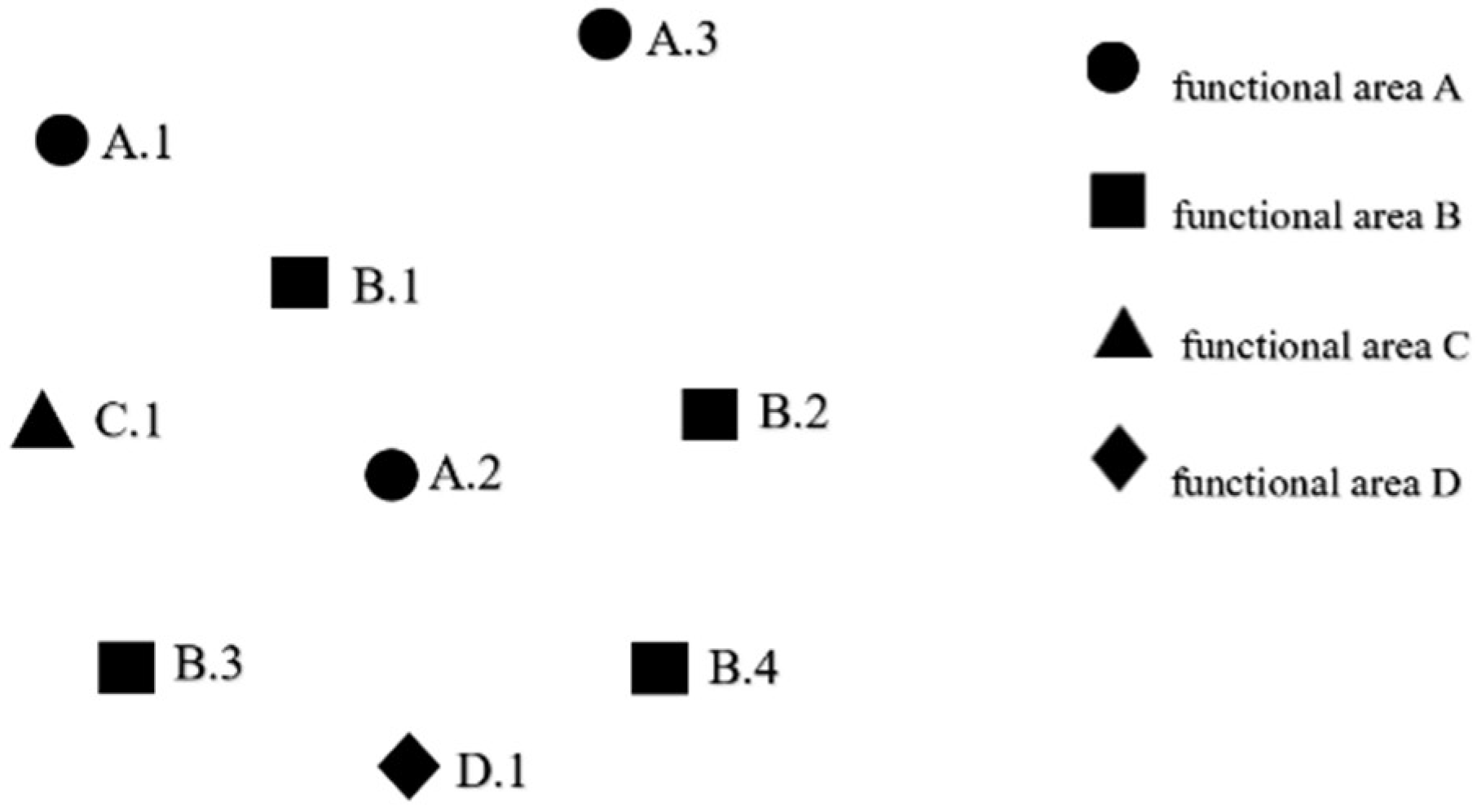
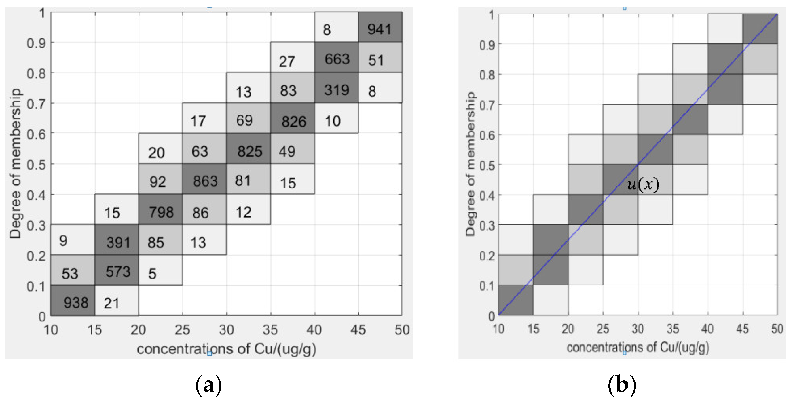
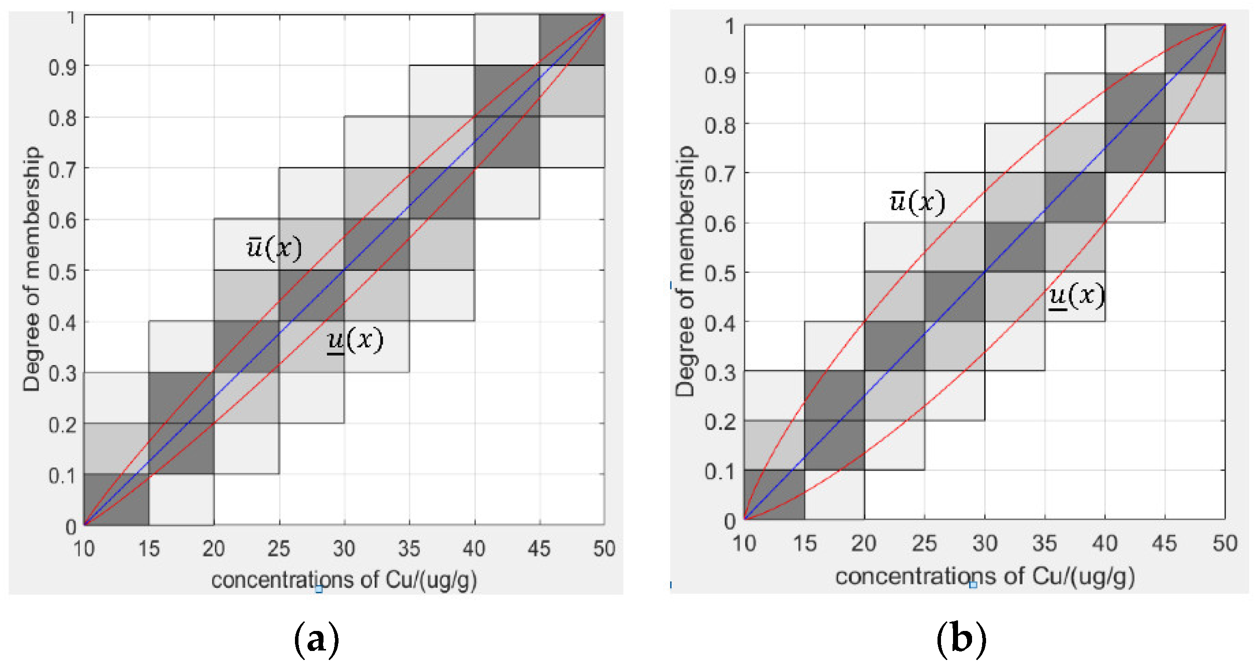
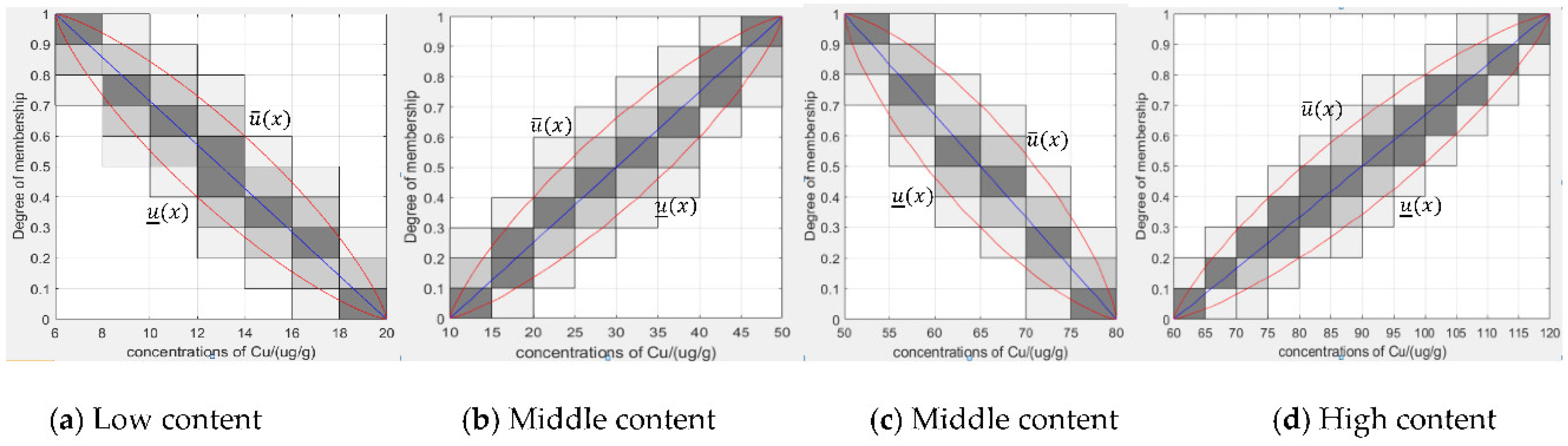
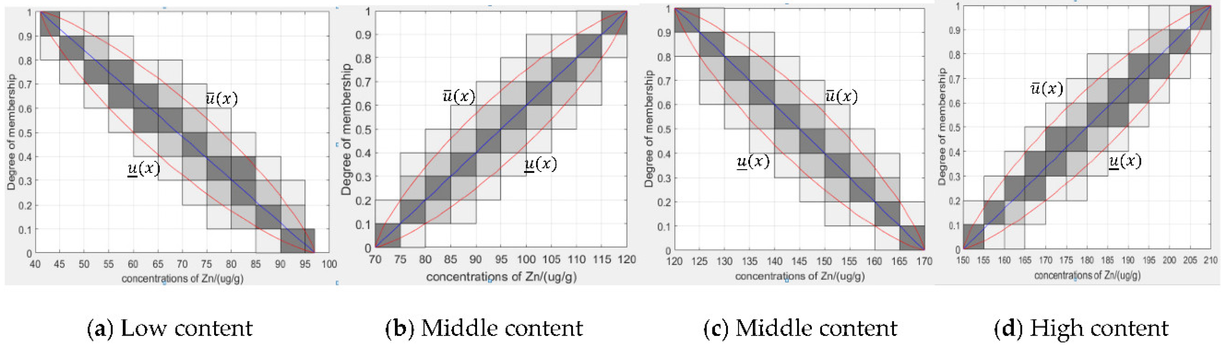
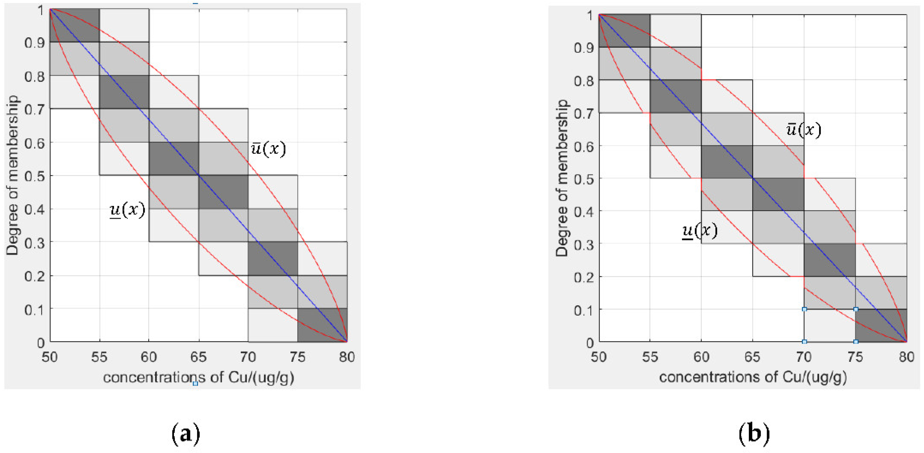
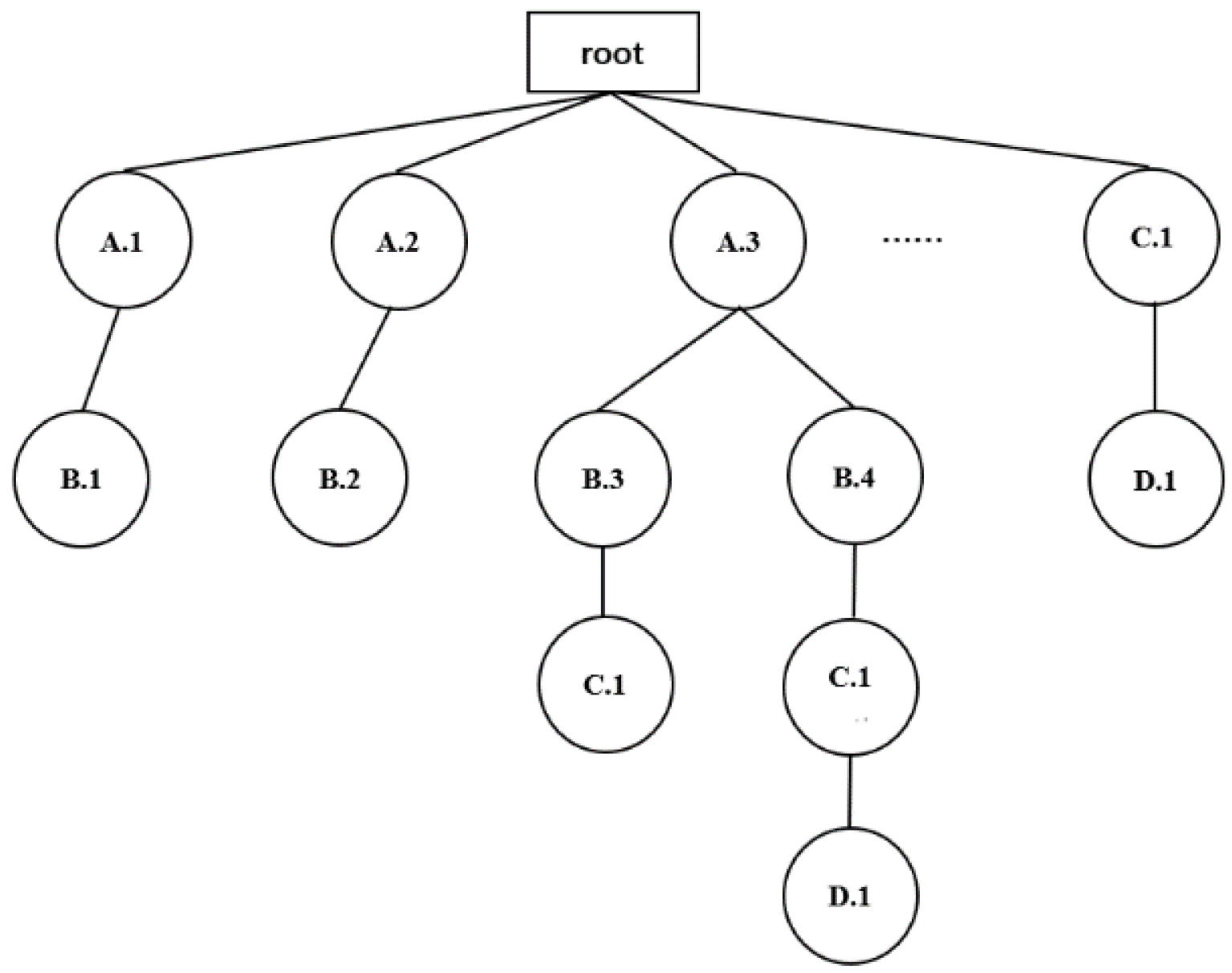
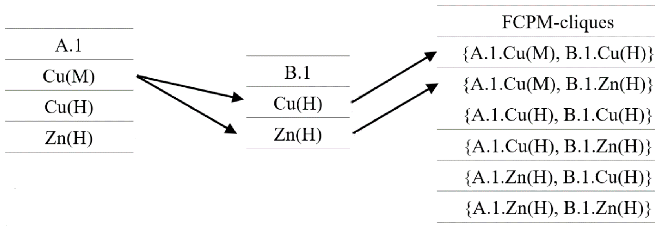
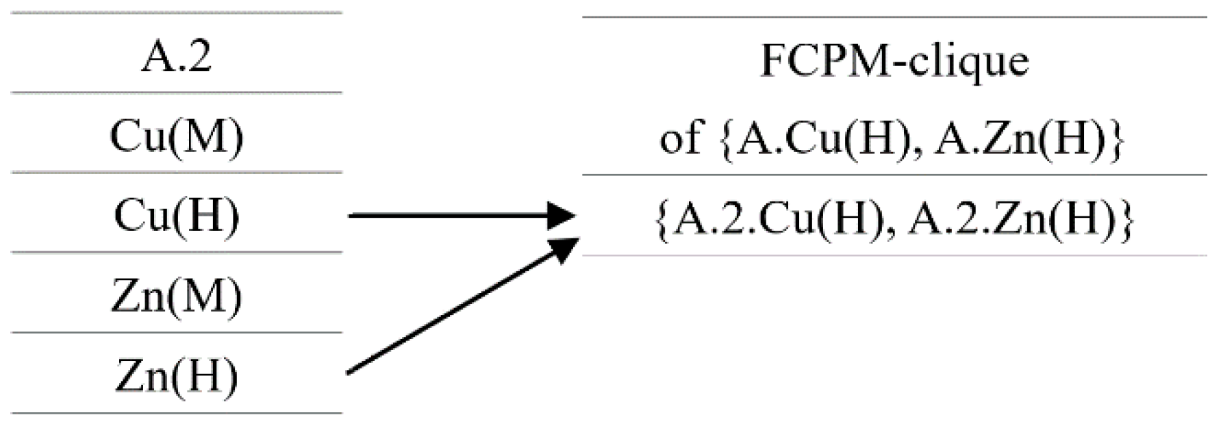
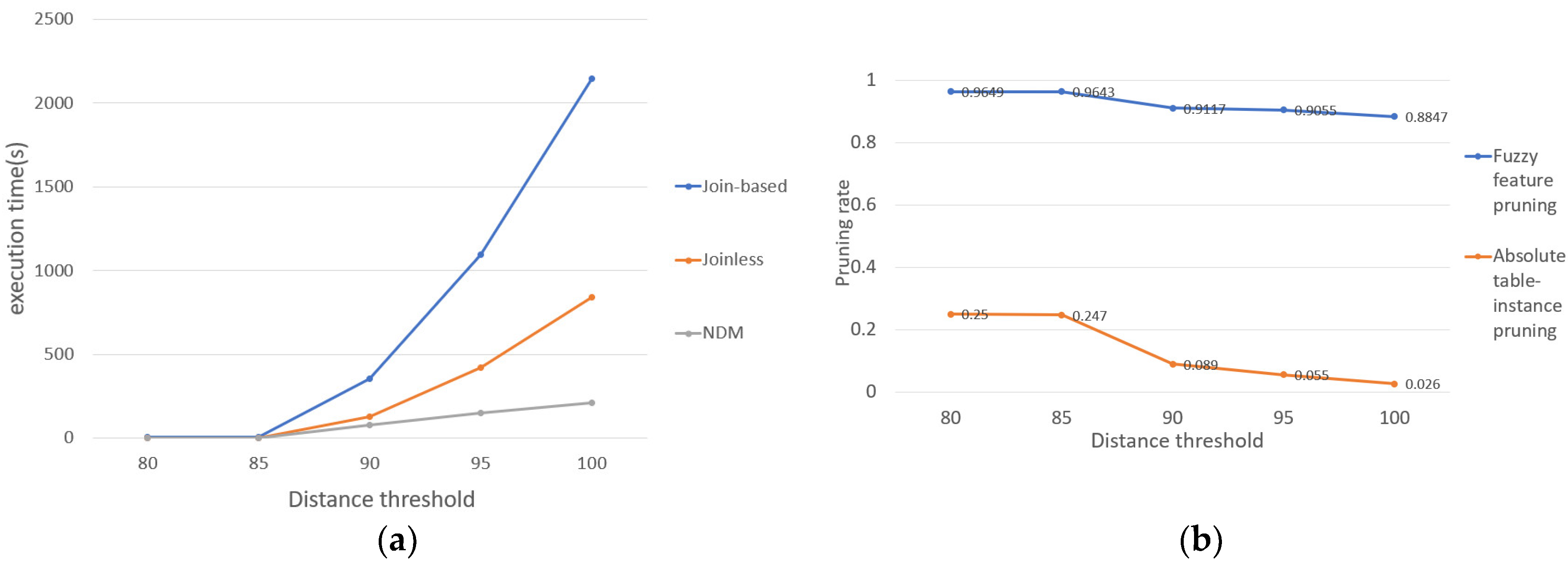
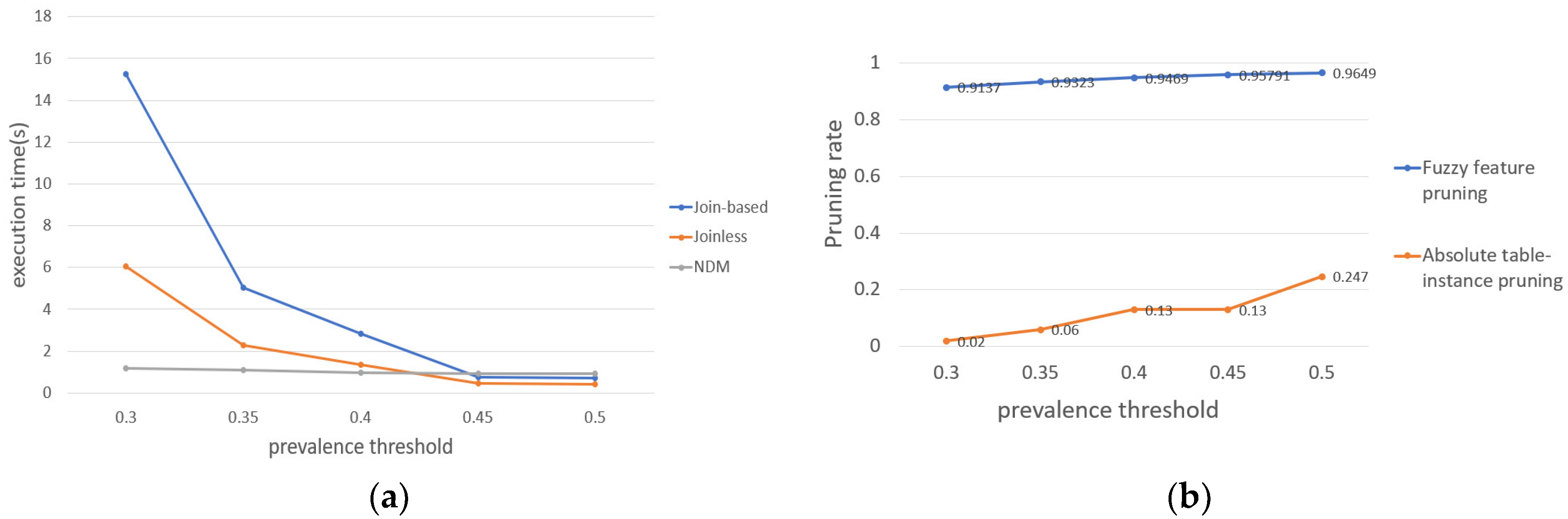
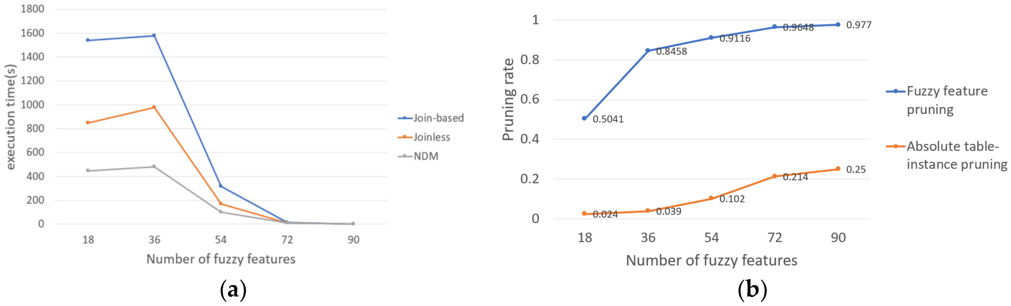
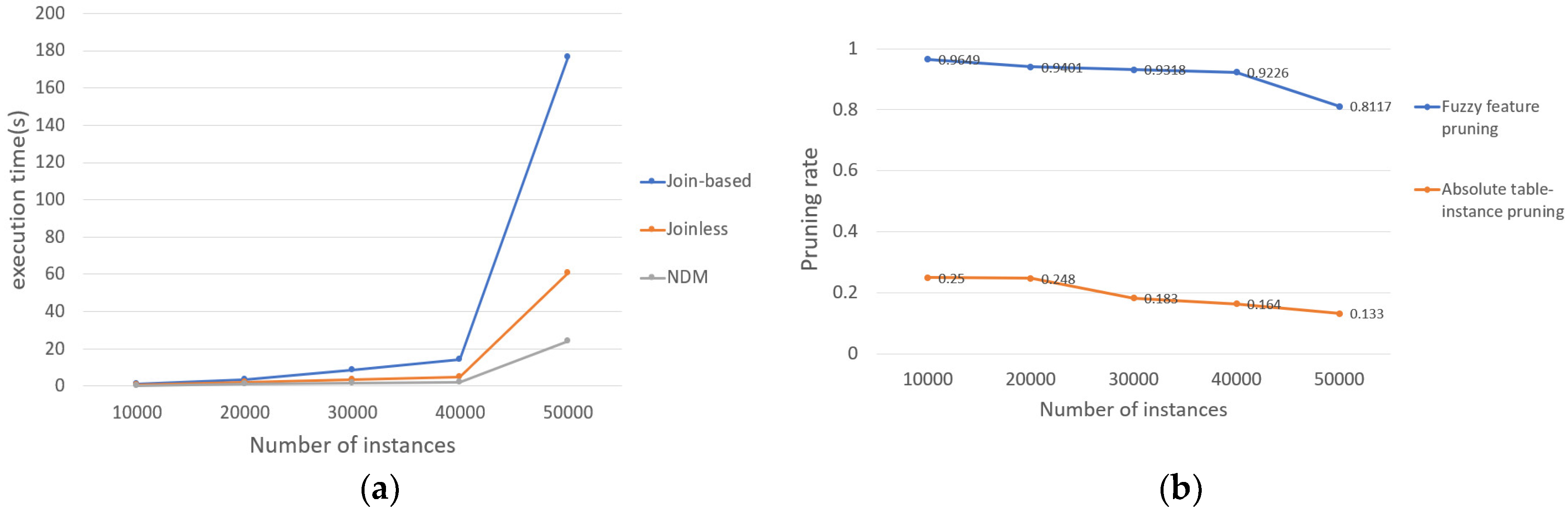
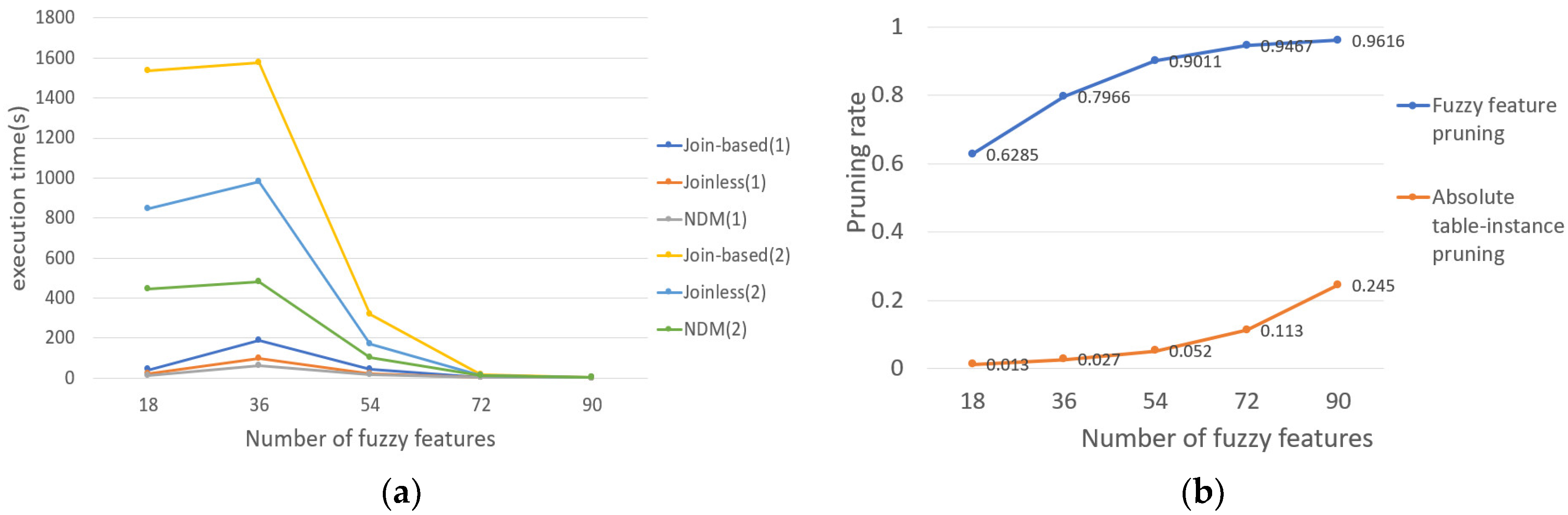
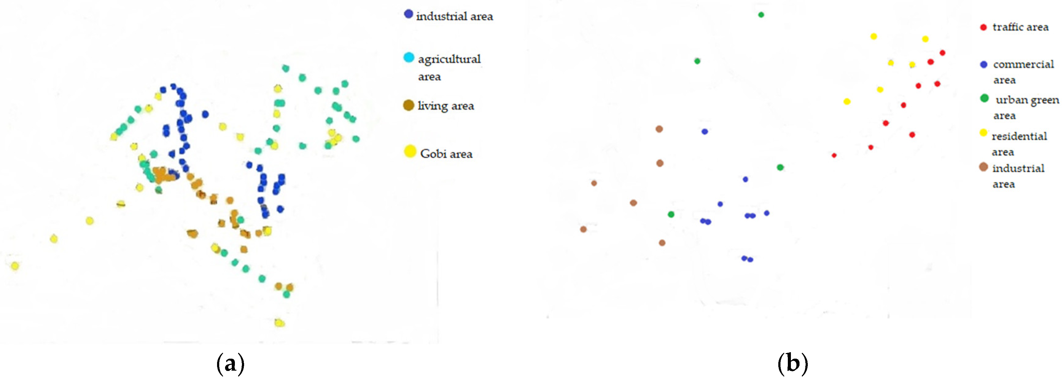
Table 1.
Attribute information of sampling points.
| Functional Area | The Number of Sampling Points | The Content of Copper | The Content of Zinc |
|---|---|---|---|
| A | 1 | 62 | 226 |
| A | 2 | 31 | 105 |
| A | 3 | 46 | 136 |
| B | 1 | 86 | 183 |
| B | 2 | 29 | 112 |
| B | 3 | 45 | 150 |
| B | 4 | 57 | 124 |
| C | 1 | 63 | 210 |
| D | 1 | 51 | 155 |
Table 2.
The interval membership of the fuzzy attribute of the sampling point.
| Functional Area | Number of Sampling Points | Cu(L) | Cu(M) | Cu(H) | Zn(L) | Zn(M) | Zn(H) |
|---|---|---|---|---|---|---|---|
| A | 1 | 0 | [0.4403, 0.7456] | [0.0104, 0.0831] | 0 | 0 | 1 |
| A | 2 | 0 | [0.3614, 0.6848] | 0 | 0 | [0.5414, 0.8298] | 0 |
| A | 3 | 0 | [0.8, 0.9591] | 0 | 0 | [0.5191, 0.8146] | 0 |
| B | 1 | 0 | 0 | [0.283, 0.5931] | 0 | 0 | [0.3905, 0.7023] |
| B | 2 | 0 | [0.3152, 0.6386] | 0 | 0 | [0.7138, 0.9252] | 0 |
| B | 3 | 0 | [0.7633, 0.9455] | 0 | 0 | [0.2495, 0.5656] | 0 |
| B | 4 | 0 | [0.5786, 0.8991] | 0 | 0 | [0.8315, 0.9695] | 0 |
| C | 1 | 0 | [0.4069, 0.717] | [0.0174, 0.1141] | 0 | 0 | 1 |
| D | 1 | 0 | [0.9169, 0.9896] | 0 | 0 | [0.1702, 0.4586] | [0.0335, 0.1698] |
Table 3.
Connectivity of the membership function with different values of .
| 1.1 | 1.2 | 1.3 | 1.4 | 1.5 | 1.6 | 1.7 | 1.8 | 1.9 | 2.0 | |
| Is it connected? | Yes | Yes | No | No | No | No | No | No | No | No |
| 1.21 | 1.22 | 1.23 | 1.24 | 1.25 | 1.26 | 1.27 | 1.28 | 1.29 | 1.3 | |
| Is it connected? | Yes | Yes | Yes | Yes | Yes | Yes | Yes | Yes | No | No |
| 1.281 | 1.282 | 1.283 | 1.284 | 1.285 | 1.286 | 1.287 | 1.288 | 1.289 | 1.29 | |
| Is it connected? | Yes | Yes | Yes | No | No | No | No | No | No | No |
Table 4.
Neighborhood table of instances.
| SNs | Instance | BNs |
|---|---|---|
| - | A.1 | {B.1} |
| - | A.2 | {B.2} |
| - | A.3 | {B.3, B.4, C.1, D.1} |
| {A.1} | B.1 | - |
| {A.2} | B.2 | - |
| {A.3} | B.3 | {C.1} |
| {A.3} | B.4 | {C.1, D.1} |
| {A.3, B.3, B.4} | C.1 | {D.1} |
| {A.3, B.3, B.4, C.1} | D.1 | - |
Table 5.
An example of the extended Joinless algorithm.
| Phase 1 | Phase 2 | Phase 3 | ||
|---|---|---|---|---|
| Star Instances of Feature A | A | {A, B} | {A.Cu(M), B.Cu(M)} | {A.Cu(M), A.Zn(M)} |
| A.1, B.2, C.2 A.2, B.3, C.1 A.3, B.5, C.2 A.4, C.3 | A.1 A.2 A.3 A.4 | A.1, B.2 A.2, B.3 A.3, B.5 | A.1, B.2 A.2, B.3 | A.1 |
Table 6.
Part of the mining results for real dataset 1.
| Prevalent Fuzzy Co-Location Pattern | Prevalence Tendency Degree | Lower Participation Index and Upper Participation Index | Participation Index for the Traditional Method |
|---|---|---|---|
| {A.Cu(L), C.Cu(L)} | 0.6125 | 0.0709, 0.6621 | 0.2312 |
| {A.Cu(L), D.Cu(L)} | 0.2328 | 0.036, 0.3801 | 0.1169 |
| {A.Cu(M), C.Cu(M)} | 0.2636 | 0.1567, 0.3513 | 0.2384 |
| {D.Cu(M), D.Zn(H)} | 1 | 0.4781, 0.9135 | 0.6599 |
| {D.Cu(L), D.Zn(M)} | 0.9096 | 0.2414, 0.8896 | 0.6681 |
| {A.Zn(L), A.Cu(M), C.Zn(L)} | 0.2636 | 0.1567, 0.3513 | 0.2384 |
| {A.Zn(L), C.Zn(L), D.Cu(M)} | 0.2167 | 0.1749, 0.3346 | 0.2492 |
| {B.Cu(L), B.Zn(L), C.Zn(L)} | 0.8586 | 0.2597, 0.5448 | 0.4342 |
| {B.Cu(M), B.Zn(L), C.Cu(M), C.Zn(M)} | 0.7039 | 0.1804, 0.5844 | 0.3358 |
| {B.Cu(M), B.Zn(L), C.Cu(M), C.Zn(L)} | 1 | 0.3933, 0.738 | 0.5726 |
Table 7.
Part of the mining results for real dataset 2.
| Prevalent Fuzzy Co-Location Pattern | Prevalence Tendency Degree | Lower Participation Index and Upper Participation Index | Participation Index for the Traditional Method |
|---|---|---|---|
| {A.Cu(M), A.Zn(M)} | 0.7965 | 0.2438, 0.5199 | 0.3661 |
| {A.Zn(H), D.Zn(H)} | 1 | 0.4114, 0.966 | 0.8528 |
| {A.Cu(M), D.Zn(H)} | 0.8208 | 0.2438, 0.5575 | 0.3661 |
| {E.Cu(L), E.Zn(L)} | 1 | 0.3657, 0.4952 | 0.4425 |
| {A.Cu(M), A.Zn(M), D.Cu(M)} | 0.7965 | 0.2438, 0.5199 | 0.3661 |
| {A.Cu(M), A.Zn(H), D.Zn(M)} | 0.9047 | 0.2828, 0.4633 | 0.3853 |
| {A.Cu(M), A.Zn(M), D.Cu(M), D.Zn(H)} | 0.7965 | 0.2438, 0.5199 | 0.3661 |
| {A.Cu(M), A.Zn(H), D.Cu(M), D.Zn(H)} | 0.9047 | 0.2828, 0.4633 | 0.3853 |
Publisher’s Note: MDPI stays neutral with regard to jurisdictional claims in published maps and institutional affiliations. |
© 2022 by the authors. Licensee MDPI, Basel, Switzerland. This article is an open access article distributed under the terms and conditions of the Creative Commons Attribution (CC BY) license (https://creativecommons.org/licenses/by/4.0/).
Share and Cite
MDPI and ACS Style
Guo, J.; Wang, L. A Spatial Fuzzy Co-Location Pattern Mining Method Based on Interval Type-2 Fuzzy Sets. Appl. Sci. 2022, 12, 6259. https://0-doi-org.brum.beds.ac.uk/10.3390/app12126259
AMA Style
Guo J, Wang L. A Spatial Fuzzy Co-Location Pattern Mining Method Based on Interval Type-2 Fuzzy Sets. Applied Sciences. 2022; 12(12):6259. https://0-doi-org.brum.beds.ac.uk/10.3390/app12126259
Chicago/Turabian StyleGuo, Jinyu, and Lizhen Wang. 2022. "A Spatial Fuzzy Co-Location Pattern Mining Method Based on Interval Type-2 Fuzzy Sets" Applied Sciences 12, no. 12: 6259. https://0-doi-org.brum.beds.ac.uk/10.3390/app12126259
Note that from the first issue of 2016, this journal uses article numbers instead of page numbers. See further details here.