
Integrated Earthquake Catalog of the Eastern Sector of the Russian Arctic

 , , and
Abstract
:1. Introduction
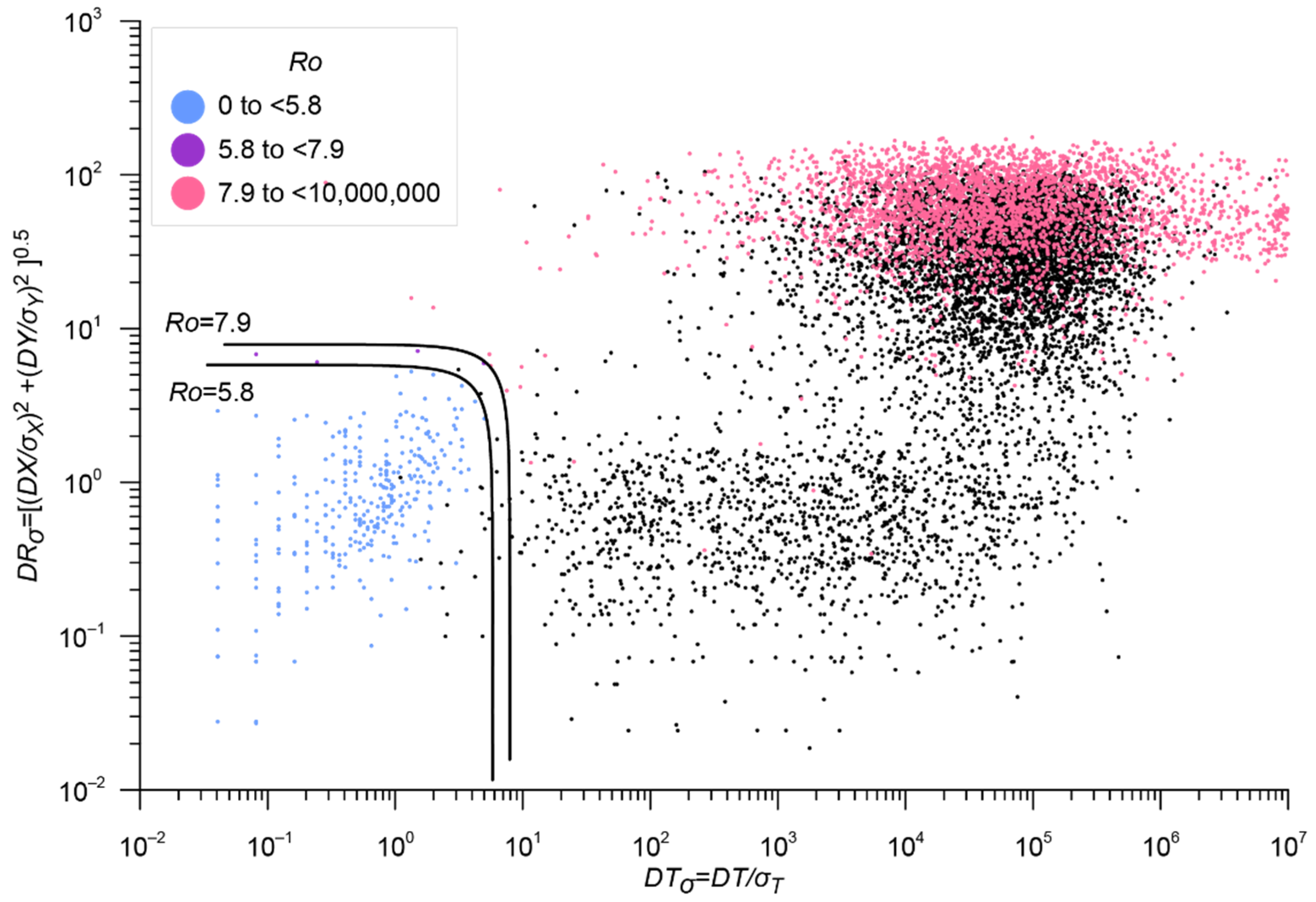
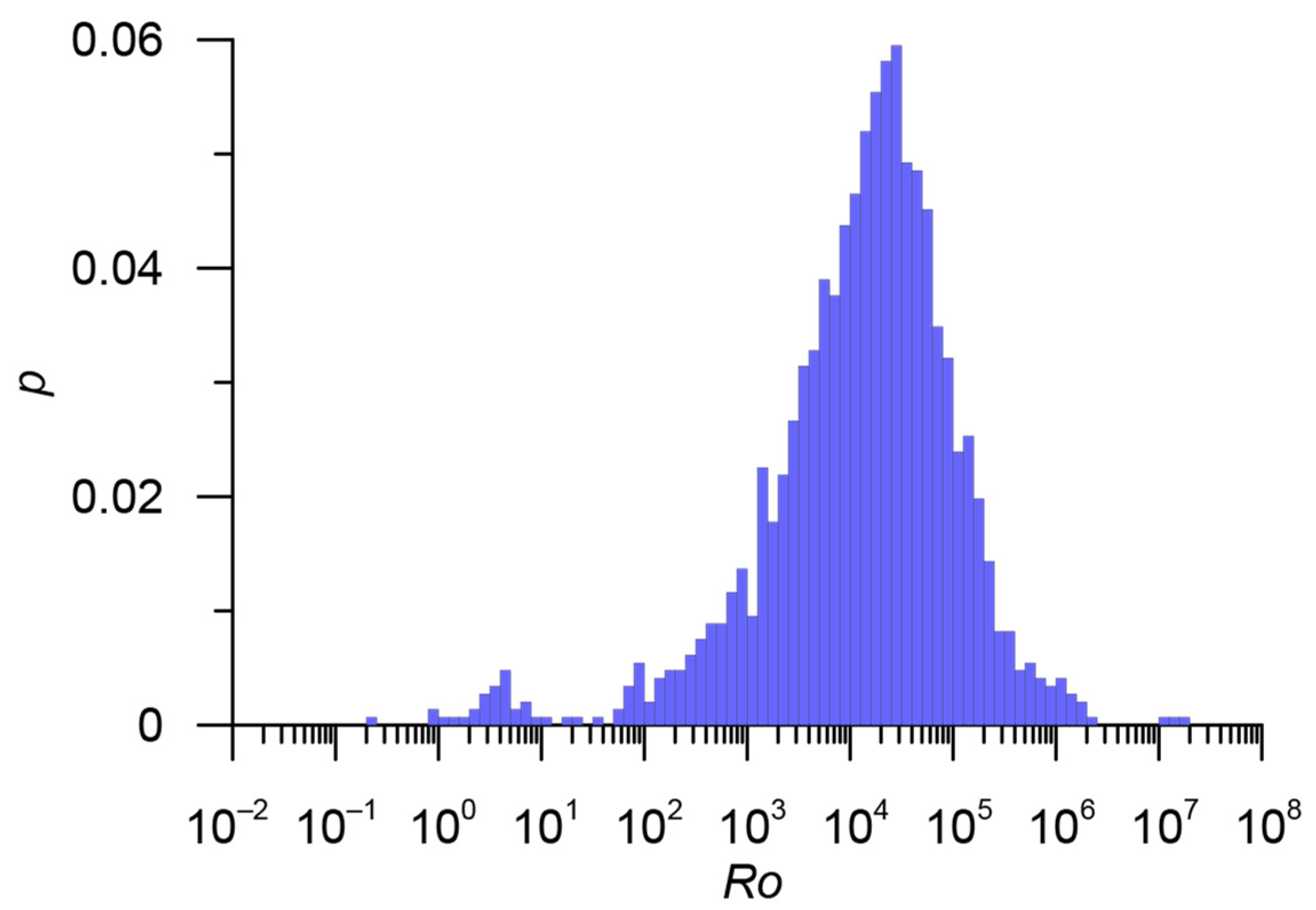
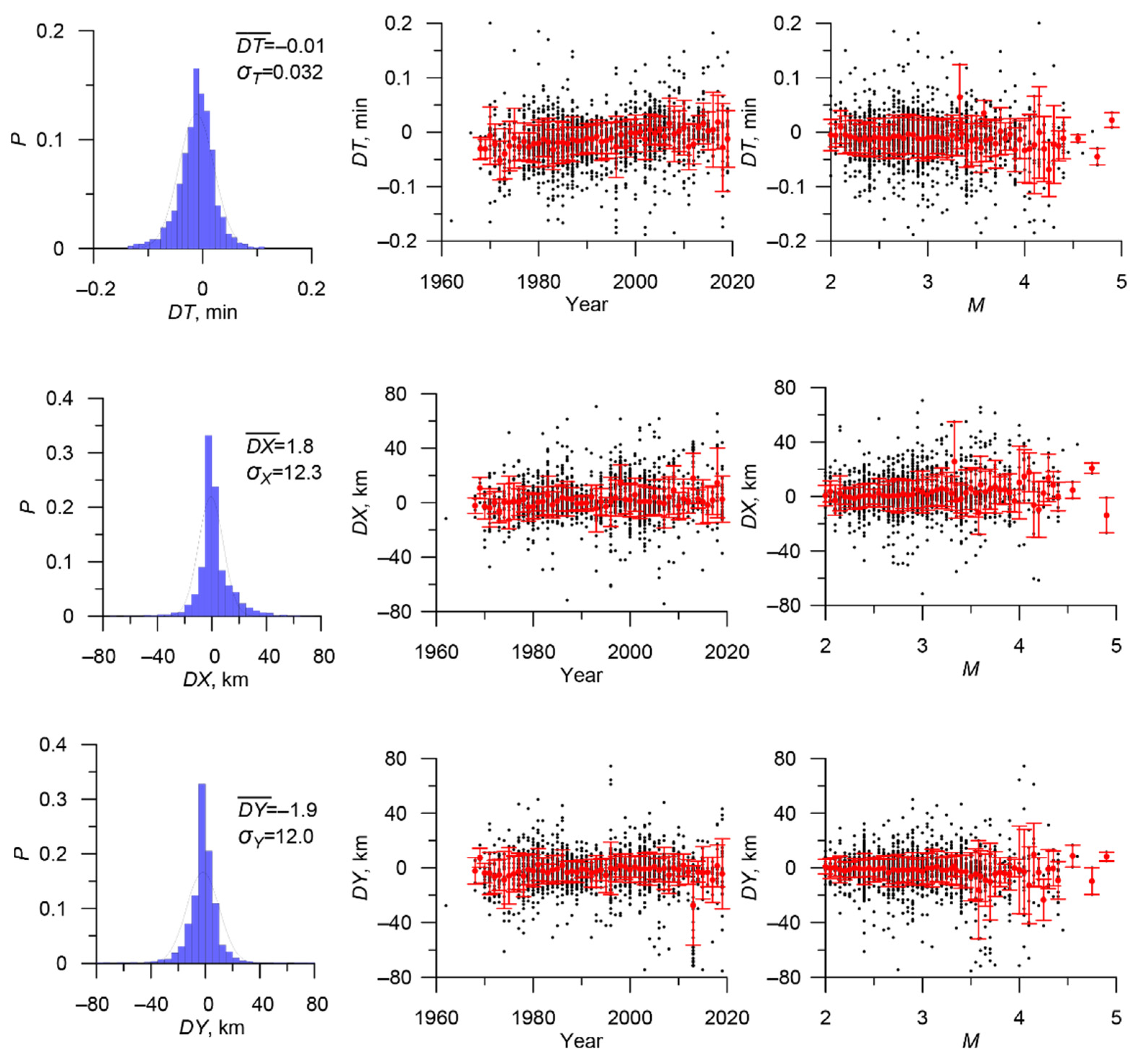
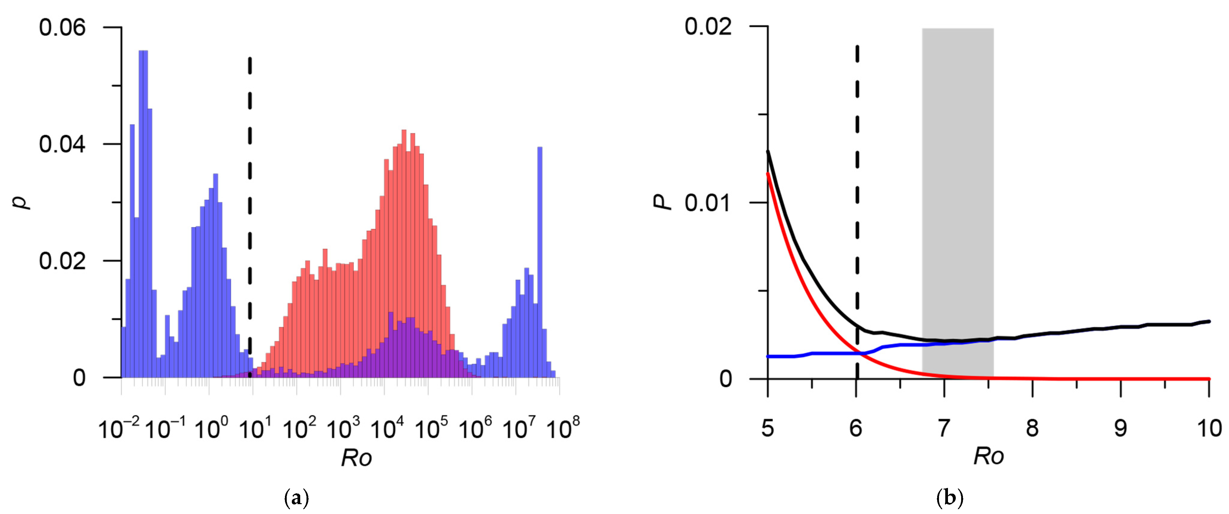
- The sequential merging of three regional catalogs of the GS RAS and the ISC catalog, which implies the identification of duplicate events in the border areas of responsibility of the different networks; and
- The unification of magnitude estimates in the integrated catalog by constructing regression relationships for the different types of magnitude/energy class due to the exact association of data from the different catalogs related to the same event.
2. Materials and Methods
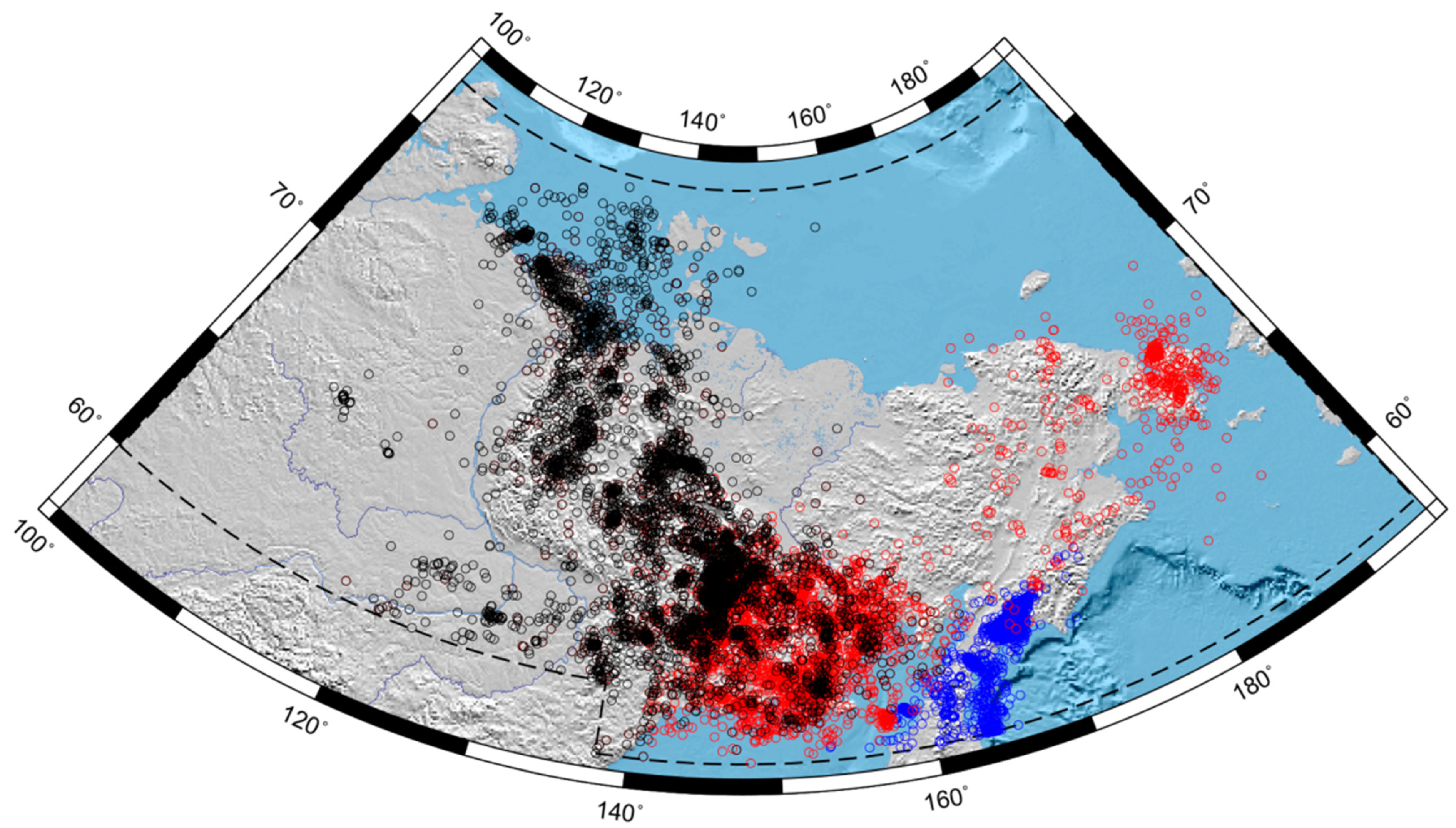
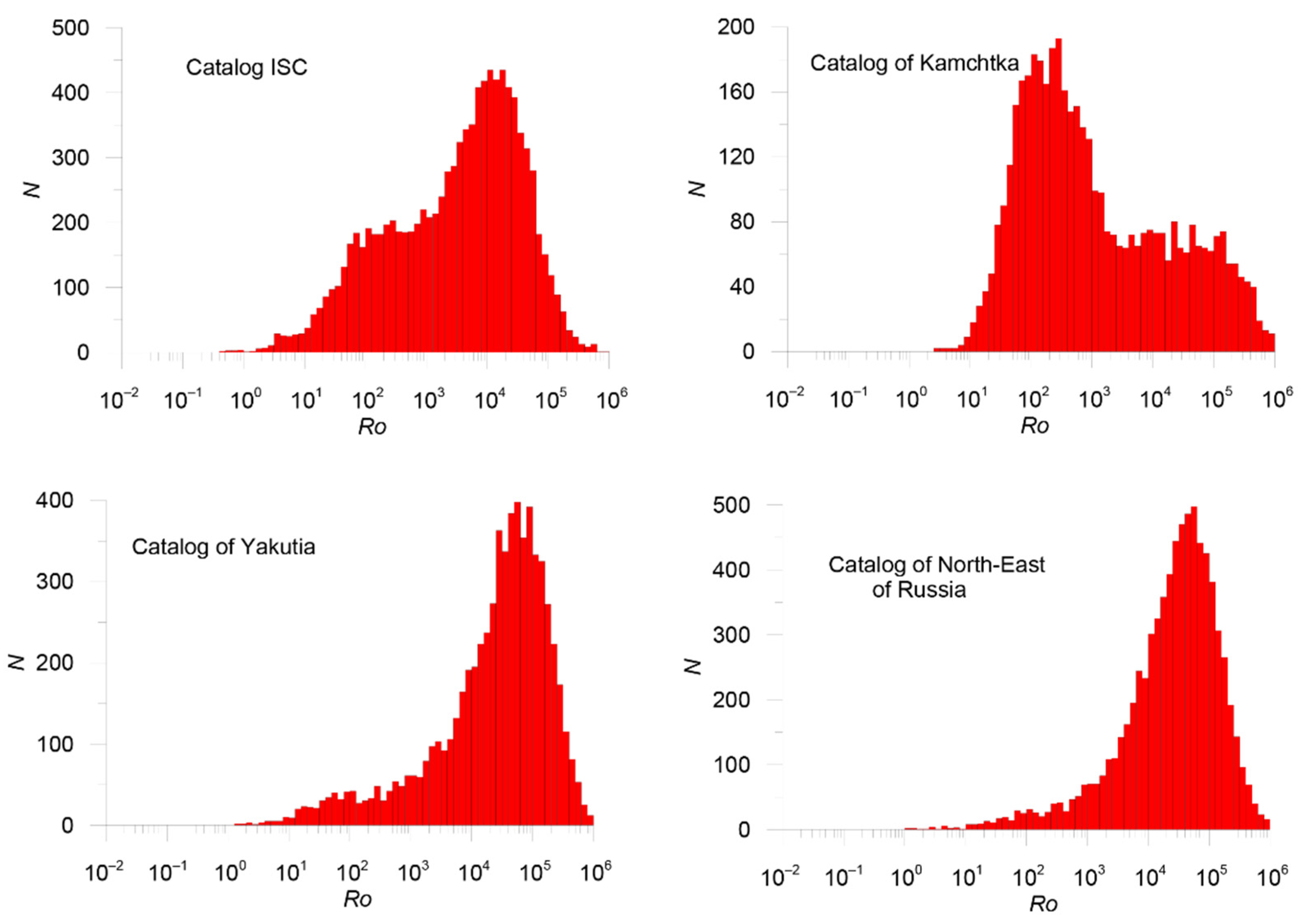
- The regional catalog of Yakutia from the annual journals Earthquakes in the USSR (1962–1991), Earthquakes in Northern Eurasia (1992–2014), and Earthquakes in Russia (2015–2019) (GS RAS) (hereinafter YAK);
- The regional catalog of the northeast of Russia from the annual journals Earthquakes in the USSR (1968–1991), Earthquakes in Northern Eurasia (1992–2014), and Earthquakes of Russia (2015–2019) (GS RAS) (hereinafter NER);
- The regional catalog of earthquakes in Kamchatka of the Kamchatka Branch of the GS RAS, 1962–2019 (hereinafter KAM); and
- The ISC 1962–2020 catalog, which is a composite catalog containing data from many world and Russian agencies.
- Earthquakes from the ISC global catalog (the abbreviation of the ISC and GCMT agency in Table 2) with the magnitudes MWGCMT and/or mbISC are the core (hereinafter CORE) (1393 events);
- Earthquakes from Russian catalogs with local estimates for the magnitude of weak events. In the intersection zones, preference is given to the data from the catalog of Yakutia (Table 1);
- Other earthquakes from the ISC (abbreviation of the ISC agency in Table 2, without the magnitude data MWGCMT or mbISC), as well as data from other agencies in the ISC catalog (16,642 events). This selection from the ISC catalog will be further denoted by ISC_Other.
3. Results
3.1. Merging Catalogs
3.1.1. Stage 1. Merging YAK and NER
3.1.2. Stage 2. Merging YAK_NER and KAM into the RUS Catalog
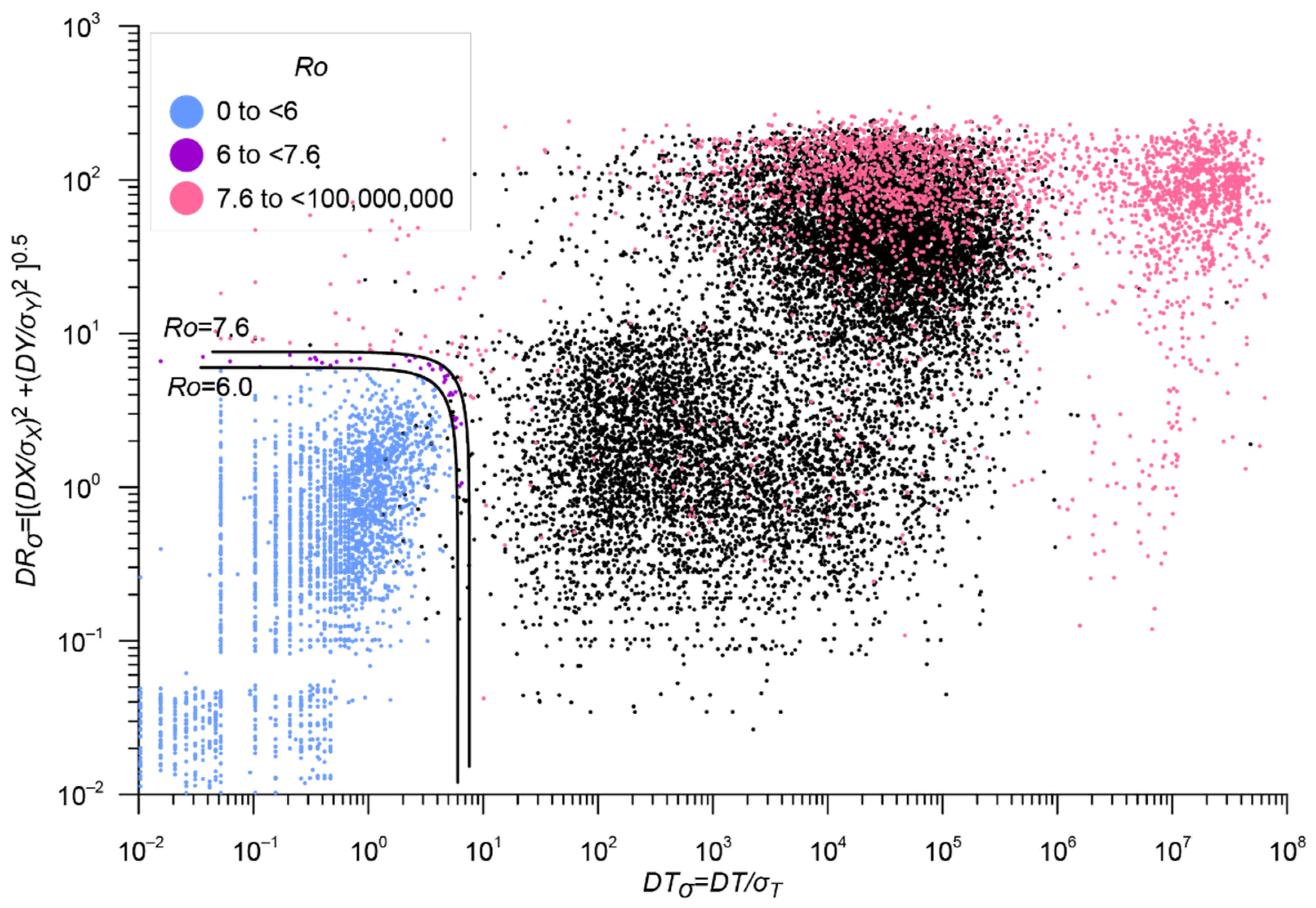
3.1.3. Stage 3. Merging RUS and Data from the ISC_Other Catalog
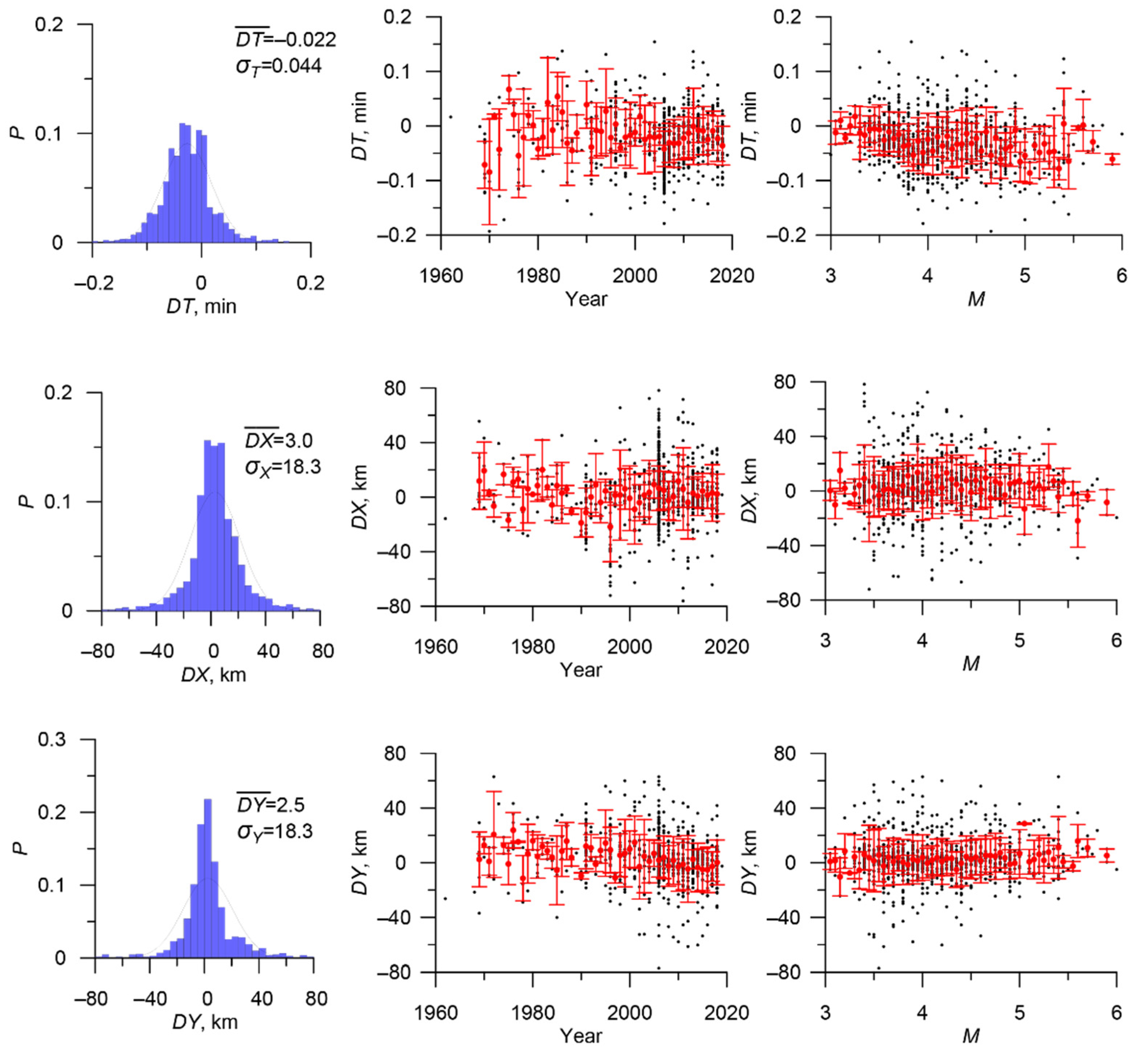
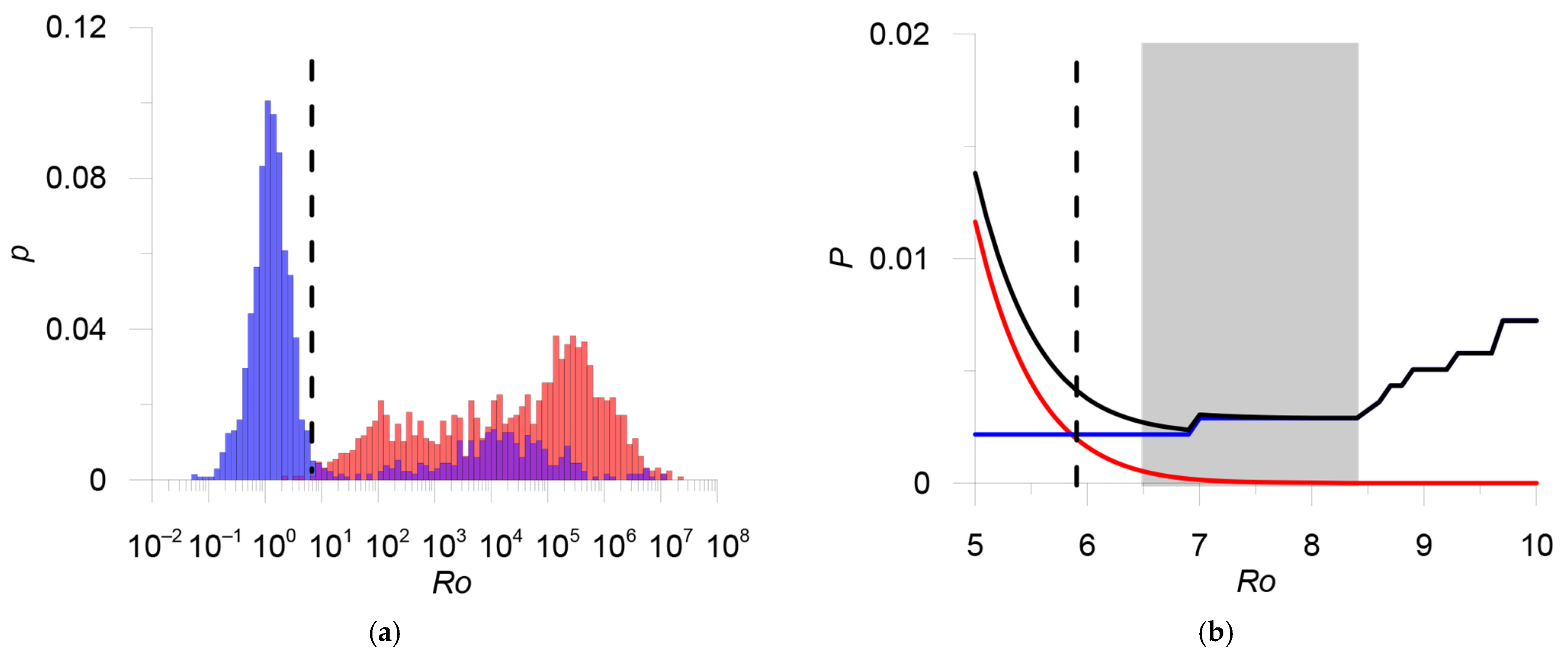
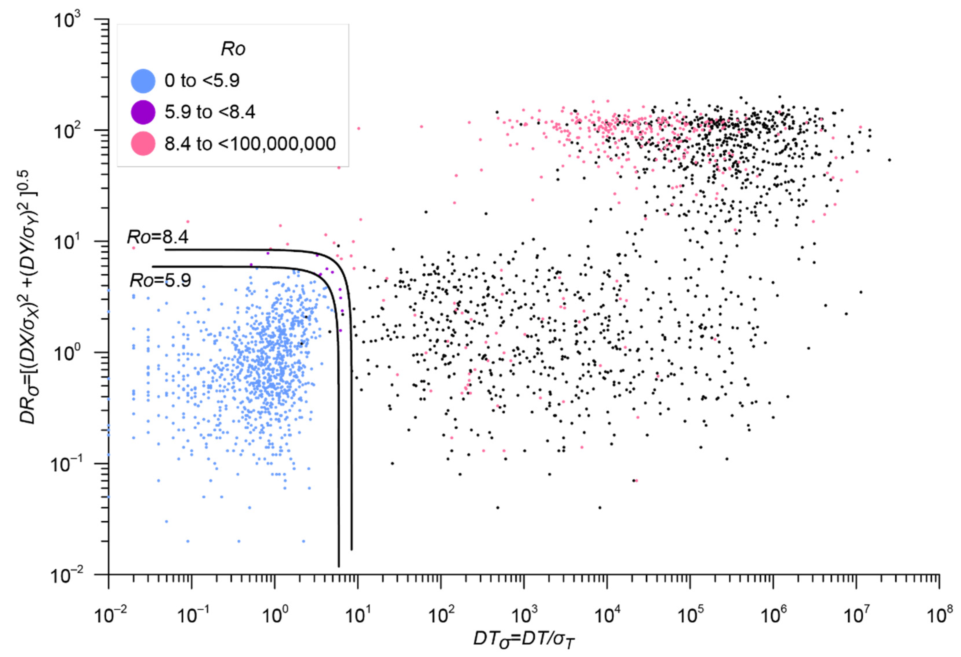
3.1.4. Stage 4. Merging RUS_ISC and CORE
3.1.5. Stage 5. Exclusion of Explosions
3.2. Magnitudes in the Integrated Catalog of the Eastern Sector of the Russian Arctic
- MWGCMT or MSISC for strong earthquakes before 1976;
- mbISC;
- Magnitude by energy class; and
- Other magnitudes.
4. Conclusions
Author Contributions
Funding
Institutional Review Board Statement
Informed Consent Statement
Data Availability Statement
Acknowledgments
Conflicts of Interest
References
- Imaeva, L.P.; Imaev, V.S.; Koz’min, B.M. Dynamics of the Zones of Strong Earthquake Epicenters in the Arctic–Asian Seismic Belt. Geosciences 2019, 9, 168. [Google Scholar] [CrossRef] [Green Version]
- Daragan-Sushchova, L.A.; Petrov, O.V.; Sobolev, N.N.; Daragan-Sushchov, Y.I.; Grin’ko, L.R.; Petrovskaya, N.A. Geology and tectonics of the northeast Russian Arctic region, based on seismic data. Geotectonics 2015, 49, 469–484. [Google Scholar] [CrossRef]
- Kanao, M.; Suvorov, V.; Toda, S.; Tsuboi, S. Seismicity, structure and tectonics in the Arctic region. Geosci. Front. 2015, 6, 665–677. [Google Scholar] [CrossRef] [Green Version]
- Skorkina, A.A. Scaling of two corner frequencies of source spectra for earthquakes of the Bering fault. Russ. J. Earth Sci. 2020, 20, ES2001. [Google Scholar] [CrossRef]
- Imaev, V.S.; Imaeva, L.P.; Koz’min, B.M. Strong Ulakhan-Chistay earthquake (Ms = 5.7) January 20, 2013 in the zone of influence Ulakhan fault system in North East Russia. Vestn. St. Petersburg Univer. Earth Sci. 2020, 65, 740–759. (In Russian) [Google Scholar] [CrossRef]
- Shibaev, S.V.; Kozmin, B.M.; Imaev, V.S.; Imaeva, L.P.; Petrov, A.F.; Starkova, N.N. The February 14, 2013 Ilin-Tas (Abyi) earthquake (Mw = 6.7), Northeast Yakutia. Russ. J. Seismol. 2020, 2, 92–102. [Google Scholar] [CrossRef]
- Chebrov, V.N. The Olyutorskii earthquake of April 20, 2006: Organizing surveys, observations, problems, and results. J. Volcanol. Seismol. 2010, 4, 75–78. [Google Scholar] [CrossRef]
- Rogozhin, E.A.; Ovsyuchenko, A.N.; Marakhanov, A.V.; Novikov, S.S. A geological study of the epicentral area of the April 20(21), 2006 Olyutorskii earthquake. J. Volcanol. Seismol. 2010, 4, 79–86. [Google Scholar] [CrossRef]
- Lander, A.V.; Levina, V.I.; Ivanova, E.I. The earthquake history of the Koryak Upland and the aftershock process of the MW7.6 April 20(21), 2006 Olyutorskii earthquake. J. Volcanol. Seismol. 2010, 4, 87–100. [Google Scholar] [CrossRef]
- Dzeboev, B.A.; Agayan, S.M.; Zharkikh, Y.I.; Krasnoperov, R.I.; Barykina, Y.V. Strongest Earthquake-Prone Areas in Kamchatka. Izv. Phys. Solid Earth 2018, 54, 284–291. [Google Scholar] [CrossRef]
- Dzeboev, B.A.; Gvishiani, A.D.; Belov, I.O.; Agayan, S.M.; Tatarinov, V.N.; Barykina, Y.V. Strong Earthquake-Prone Areas Recognition Based on an Algorithm with a Single Pure Training Class: I. Altai-Sayan-Baikal Region, M ≥ 6.0. Izv. Phys. Solid Earth 2019, 55, 563–575. [Google Scholar] [CrossRef]
- Dzeboev, B.A.; Karapetyan, J.K.; Aronov, G.A.; Dzeranov, B.V.; Kudin, D.V.; Karapetyan, R.K.; Vavilin, E.V. FCAZ-recognition based on declustered earthquake catalogs. Russ. J. Earth Sci. 2020, 20, ES6010. [Google Scholar] [CrossRef]
- Gorshkov, A.I.; Soloviev, A.A. Recognition of earthquake-prone areas in the Altai-Sayan-Baikal region based on the morphostructural zoning. Russ. J. Earth Sci. 2021, 21, ES1005. [Google Scholar] [CrossRef]
- Gvishiani, A.; Dobrovolsky, M.; Agayan, S.; Dzeboev, B. Fuzzy-based clustering of epicenters and strong earthquake-prone areas. Environ. Eng. Manag. J. 2013, 12, 1–10. [Google Scholar]
- Gvishiani, A.D.; Dzeboev, B.A.; Agayan, S.M. FCAZm intelligent recognition system for locating areas prone to strong earthquakes in the Andean and Caucasian Mountain belts. Izv. Phys. Solid Earth 2016, 52, 461–491. [Google Scholar] [CrossRef]
- Gvishiani, A.D.; Dzeboev, B.A.; Sergeyeva, N.A.; Belov, I.O.; Rybkina, A.I. Significant Earthquake-Prone Areas in the Altai–Sayan Region. Izv. Phys. Solid Earth 2018, 54, 406–414. [Google Scholar] [CrossRef]
- Gvishiani, A.D.; Soloviev, A.A.; Dzeboev, B.A. Problem of Recognition of Strong-Earthquake-Prone Areas: A State-of-the-Art Review. Izv. Phys. Solid Earth 2020, 56, 1–23. [Google Scholar] [CrossRef]
- Levin, B.W.; Kim, C.U.; Solovjev, V.N. A seismic hazard assessment and the results of detailed seismic zoning for urban territories of Sakhalin Island. Russ. J. Pac. Geol. 2013, 7, 455–464. [Google Scholar] [CrossRef]
- Lunina, O.V.; Gladkov, A.S.; Gladkov, A.A. Systematization of active faults for the assessment of the seismic hazard. Russ. J. Pac. Geol. 2012, 6, 42–51. [Google Scholar] [CrossRef]
- Magrin, A.; Peresan, A.; Kronrod, T.; Vaccari, F.; Panza, G.F. Neo-deterministic seismic hazard assessment and earthquake occurrence rate. Eng. Geol. 2017, 229, 95–109. [Google Scholar] [CrossRef]
- Nekrasova, A.; Kossobokov, V.G.; Parvez, I.A.; Tao, X. Seismic hazard and risk assessment based on the unified scaling law for earthquakes. Acta Geod. Et Geophys. 2015, 50, 21–37. [Google Scholar] [CrossRef] [Green Version]
- Ulomov, V.I. Seismic hazard of Northern Eurasia. Ann. Di Geofis. 1999, 42, 1023–1038. [Google Scholar] [CrossRef]
- Zaalishvili, V.; Chernov, Y.K. Methodology of detailed assessment of the seismic hazard of the Republic of North Ossetia-Alania. Open Constr. Build. Technol. J. 2018, 12, 309–318. [Google Scholar] [CrossRef]
- Zaalishvili, V.B.; Rogozhin, E.A. Assessment of seismic hazard of territory on basis of modern methods of detailed zoning and seismic microzonation. Open Constr. Build. Technol. J. 2011, 5, 30–40. [Google Scholar] [CrossRef] [Green Version]
- Zavyalov, A.D.; Peretokin, S.A.; Danilova, T.I.; Medvedeva, N.S.; Akatova, K.N. General Seismic Zoning: From Maps GSZ-97 to GSZ-2016 and New-Generation Maps in the Parameters of Physical Characteristics. Seism. Instr. 2019, 55, 445–463. [Google Scholar] [CrossRef]
- Beauval, C.; Yepes, H.; Palacios, P.; Segovia, M.; Alvarado, A.; Font, Y.; Aguilar, J.; Troncoso, L.; Vaca, S. An Earthquake Catalog for Seismic Hazard Assessment in Ecuador. Bull. Seismol. Soc. Am. 2013, 103, 773–786. [Google Scholar] [CrossRef]
- Kondorskaya, N.V.; Shebalin, N.V. (Eds.) New Catalog of Strong Earthquakes in the USSR from Ancient Times through 1977; Report SE-31; World Data Center A for Solid Earth Geophysics: Boulder, CO, USA, 1982; 608p. [Google Scholar]
- Shebalin, P.N. Compilation of earthquake catalogs as a task of clustering analysis with learning. Dokl. Akad. Nauk. SSSR 1987, 292, 1083–1086. [Google Scholar]
- Markušić, S.; Gülerce, Z.; Kuka, N.; Duni, L.; Ivančić, I.; Radovanović, S.; Glavatović, B.; Milutinović, Z.; Akkar, S.; Kovačević, S.; et al. An updated and unified earthquake catalogue for the Western Balkan Region. Bull. Earthq. Eng. 2016, 14, 321–343. [Google Scholar] [CrossRef]
- Sawires, R.; Santoyo, M.A.; Peláez, J.A.; Corona Fernández, R.D. An updated and unified earthquake catalog from 1787 to 2018 for seismic hazard assessment studies in Mexico. Sci. Data 2019, 6, 241. [Google Scholar] [CrossRef] [Green Version]
- Braclawska, A.; Idziak, A. Unification of data from various seismic catalogues to study seismic activity in the Carpathians Mountain arc. Open Geosci. 2019, 11, 837–842. [Google Scholar] [CrossRef]
- Long, F.; Jiang, C.; Qi, Y.; Liu, Z.; Fu, Y. A joint probabilistic approach for merging earthquake catalogs of two neighboring seismic networks: An example of the 2014 Ludian sequence catalog. Acta Geophys. Sin. 2018, 61, 2815–2827. [Google Scholar] [CrossRef]
- Muller, S.; Garda, P.; Muller, J.-D.; Cansi, Y. Seismic events discrimination by neuro-fuzzy merging of signal and catalogue features. Phys. Chem. Earth Part. A Solid Earth Geod. 1999, 24, 201–206. [Google Scholar] [CrossRef]
- Vorobieva, I.; Gvishiani, A.; Dzeboev, B.; Dzeranov, B.; Barykina, Y.; Antipova, A. Nearest Neighbor Method for Discriminating Aftershocks and Duplicates When Merging Earthquake Catalogs. Front. Earth Sci. SI Nat. Clust. Earthq. Process. Var. Scales Lab. Exp. Large Earthq. 2022, 10, 820277. [Google Scholar] [CrossRef]
- Zaliapin, I.; Ben-Zion, Y. Earthquake clusters in southern California. I: Identification and stability. J. Geophys. Res. Solid Earth 2013, 118, 2847–2864. [Google Scholar] [CrossRef]
- Zaliapin, I.; Ben-Zion, Y. A global classification and characterization of earthquake clusters. Geophys. J. Int. 2016, 207, 608–634. [Google Scholar] [CrossRef] [Green Version]
- Kanamori, H. The Energy Release in Great Earthquakes. J. Geophys. Res. 1977, 82, 2981–2987. [Google Scholar] [CrossRef] [Green Version]
- Hanks, T.C.; Kanamori, H. A Moment Magnitude Scale. J. Geophys. Res. Solid Earth 1979, 84, 2348–2350. [Google Scholar] [CrossRef]
- Di Giacomo, D.; Harris, J.; Storchak, D.A. Complementing regional moment magnitudes to GCMT: A perspective from the rebuilt International Seismological Centre Bulletin. Earth Syst. Sci. Data 2021, 13, 1957–1985. [Google Scholar] [CrossRef]
- Abubakirov, I.R.; Gusev, A.A.; Guseva, E.M.; Pavlov, V.M.; Skorkina, A.A. Mass determination of moment magnitudes Mw and establishing the relationship between Mw and ML for moderate and small Kamchatka earthquakes. Izv. Phys. Solid Earth 2018, 54, 33–47. [Google Scholar] [CrossRef]
- Di Giacomo, D.; Bondár, I.; Storchak, D.A.; Engdahl, E.R.; Bormann, P.; Harris, J. ISC-GEM: Global Instrumental Earthquake Catalogue (1900–2009), III. Re-computed MS and mb, proxy MW, final magnitude composition and completeness assessment. Phys. Earth Planet. Inter. 2015, 239, 33–47. [Google Scholar] [CrossRef]
- Rautian, T.G. Energy of earthquakes. In Methods for the Detailed Study of Seismicity; The USSR Academy of Sciences: Moscow, Russia, 1960; pp. 75–114. (In Russian) [Google Scholar]
- Rautian, T.G.; Khalturin, V.I.; Fujita, K.; Mackey, K.G.; Kendall, A.D. Origins and methodology of the Russian energy K-class system and its relationship to magnitude scales. Seismol. Res. Lett. 2007, 78, 579–590. [Google Scholar] [CrossRef]
- Fedotov, S.A. Energy Classification of the Kuril-Kamchatka Earthquakes and the Problem of Magnitudes; Nauka: Moscow, Russia, 1972; p. 117. (In Russian) [Google Scholar]
- Richter, C.F. An instrumental earthquake magnitude scale. Bull. Seismol. Soc. Am. 1935, 25, 1–32. [Google Scholar] [CrossRef]


| Catalog | Period | Number of Earthquakes with Energy Classes and/or Magnitudes | Number of Earthquakes with Unknown Energy Classes and Magnitudes |
|---|---|---|---|
| YAK | 1962, 1968–2019 | 6600 | 46 |
| NER | 1968–2019 | 7668 | 1 |
| KAM | 1962–2019 | 4498 | 0 |
| Agency Abbreviation | Agency | Number of Earthquakes with Energy Classes and/or Magnitudes * |
|---|---|---|
| AEIC | Alaska Earthquake Information Center, USA | 184 |
| ANDRE | USSR | 16 |
| ANF | USArray Array Network Facility, USA | 2 |
| BJI | China Earthquake Networks Center, China | 1 |
| BYKL | Baykal Regional Seismological Centre, GS SB RAS, Russia | 4 |
| DNAG | USA | 13 |
| EIDC | Experimental (GSETT3) International Data Center, USA | 22 |
| GCMT | The Global CMT Project, USA | 1 |
| IDC | International Data Centre, CTBTO, Austria | 123 |
| ISC | International Seismological Centre, United Kingdom | 1507 |
| KRSC | Kamchatka Branch of the Geophysical Survey of the RAS, Russia | 2684 |
| MATSS | USSR | 1400 |
| MOS | Geophysical Survey of Russian Academy of Sciences, Russia | 26 |
| MSUGS | Michigan State University, Department of Geological Sciences, USA | 2585 |
| NEIC | National Earthquake Information Center, USA | 192 |
| NEIS | National Earthquake Information Service, USA | 1 |
| NERS | North Eastern Regional Seismological Centre, GS RAS, Russia | 4688 |
| NKSZ | USSR | 8 |
| SBDV | USSR | 107 |
| SYKES | Sykes Catalogue of earthquakes 1950 onwards | 2 |
| USCGS | United States Coast and Geodetic Survey, NEIC, USA | 1 |
| WASN | USA | 328 |
| YARS | Yakutiya Regional Seismological Center, GS SB RAS, Russia | 2256 |
| ZEMSU | USSR | 1884 |
| Total: | 18,035 |
| Stage | Main Catalog | Additional Catalog | Threshold Value of the Metric | Estimation of the Number of Errors | Number of Duplicates | Merged Catalog | |
|---|---|---|---|---|---|---|---|
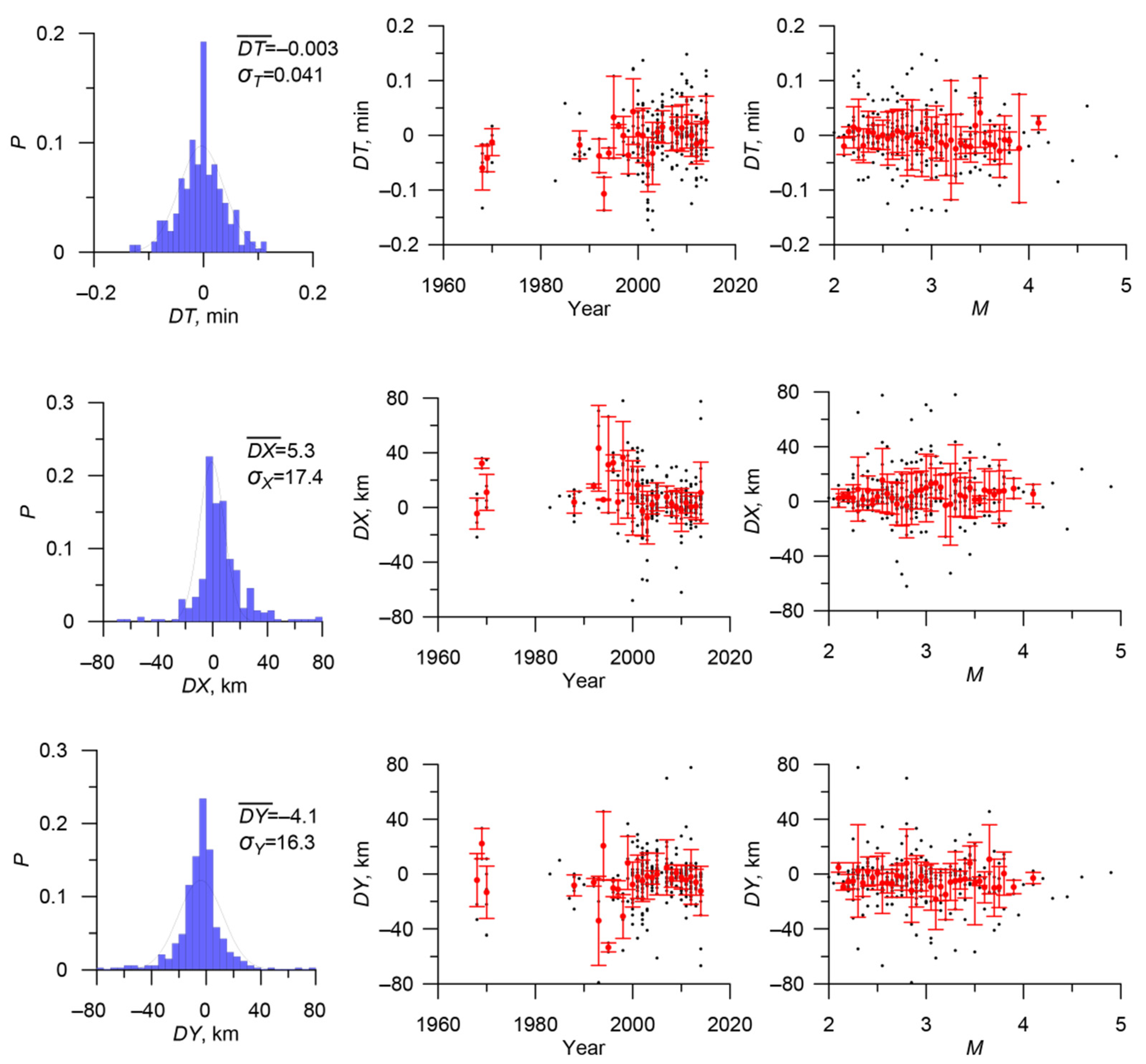
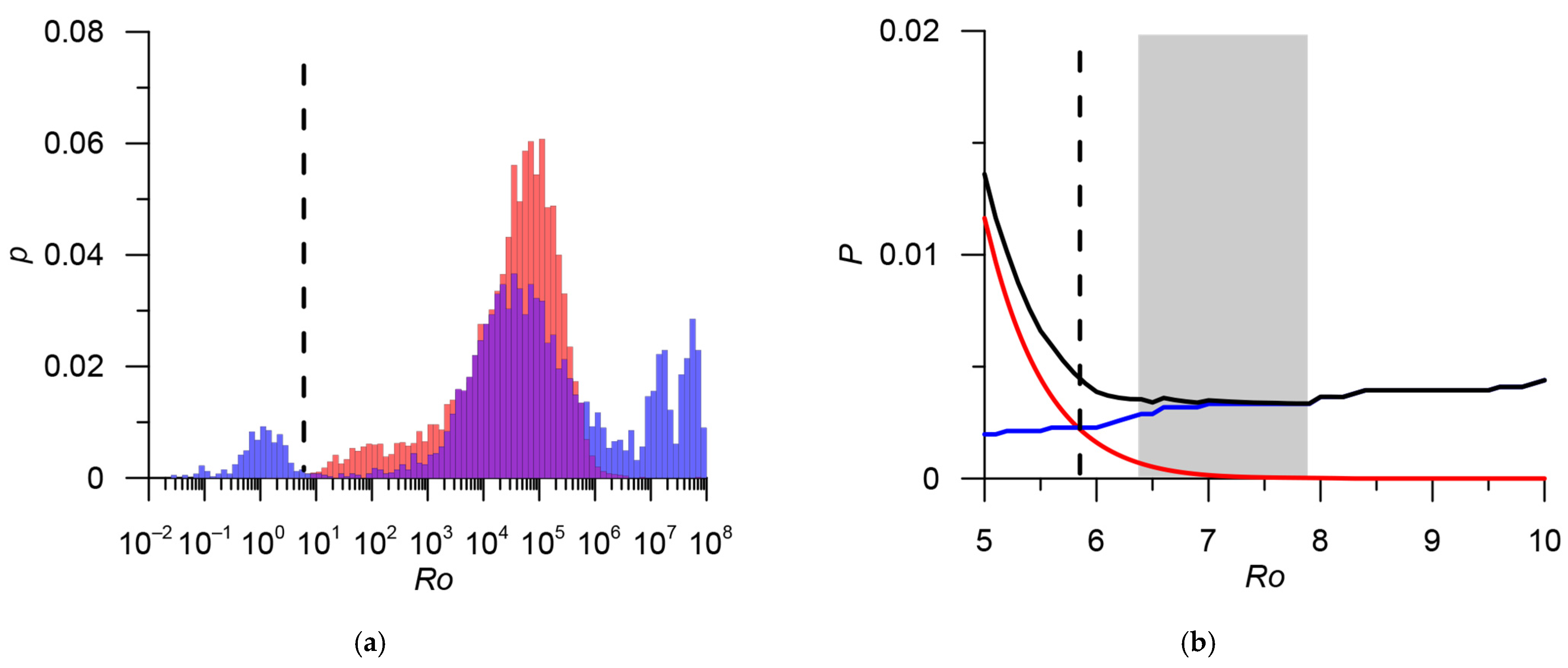
| 1 | Catalog of Yakutia YAK 6600 events | Catalog of the Northeast of Russia NER 7668 events | 0.041; 17.4; 16.3 | 5.8 | 0.5% | 2153 | YAK_NER 12,115 events |
| 2 | YAK_NER 12,115 events | Earthquake catalog of the Kamchatka Branch of the GS RAS KAM 4498 events | 0.041; 17.4; 16.3 | 5.8 * | – | 26 * | RUS 16,587 events |
| 3 | RUS 16,587 events | ISC, events of various agencies ISC_Other 16,642 events | 0.032; 12.3; 12.0 | 6.0 | 0.3% | 10,231 | RUS_ISC 22,998 events |
| 4 | CORE 1383 events | RUS_ISC 22,998 events | 0.044; 18.3; 18.3 | 5.9 | 0.4% | 1011 | ARCTIC 23,370 events |
| 5 | Exclusion of explosions EXP 116 events | ARCTIC 23,370 events | 0.05; 15.0; 15.0 | – | 0% | 116 ** | E_ARCTIC 23,254 events |
| Agency | Type of Magnitude | Priority | Number of Events | Formula for Magnitude in the Integrated Catalog | Figure | Mmin–Mmax. Initial Magnitude Scale | Note |
|---|---|---|---|---|---|---|---|
| GCMT | MW | 1 | 105 | M = MWGCMT | 4.7–7.6 | ||
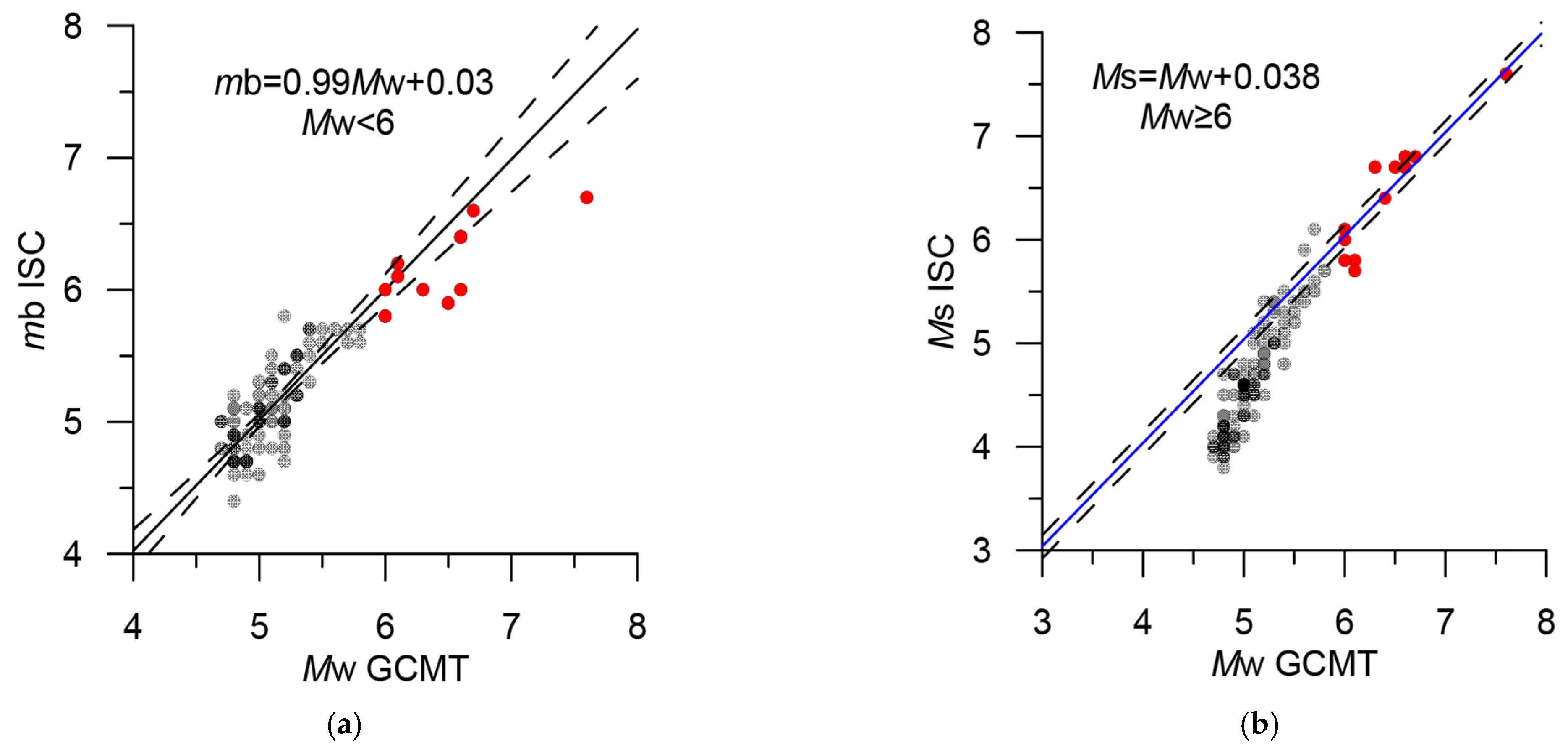
| ISC | mb | 2 | 1287 | M = mbISC | Figure 13a | 3.0–5.9 | |
| ISC | MS | 1 | 4 | M = MSISC | Figure 13b | 5.7–7.5 | Strong events before 1976 |
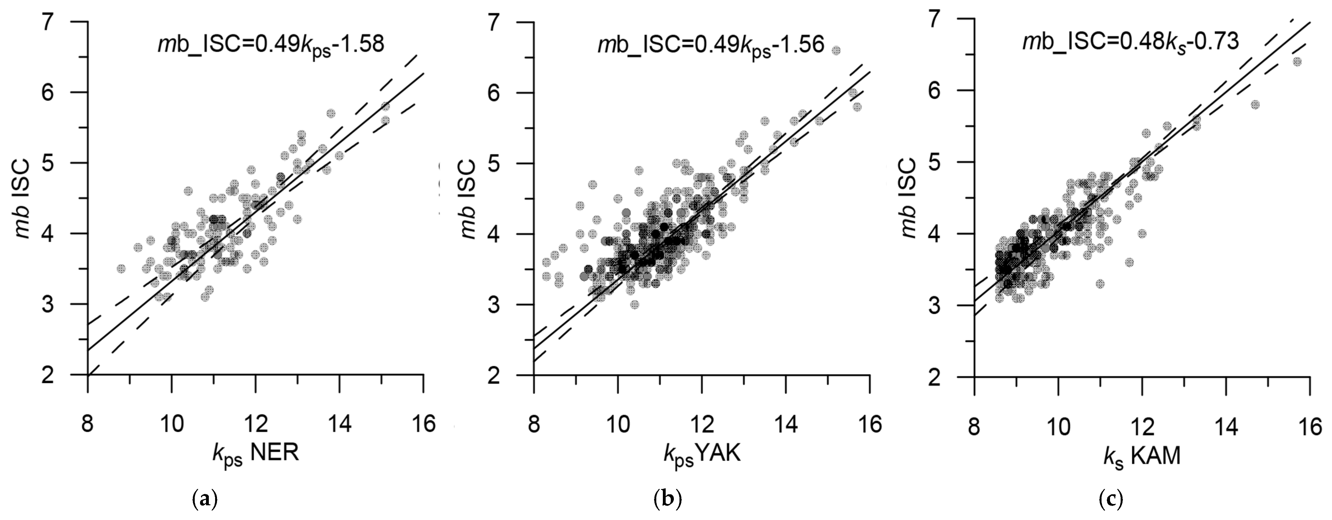
| YAK, NER, agencies of Russia and the USSR from ISC | KPS | 3 | 16,301 | M = 0.5 KPS − 1.6 | Figure 14a,b | 0.6–14.0 | Information about energy classes is given in the ISC bulletins |
| KAM, KRSC | KS | 3 | 4050 | M = 0.5KS − 0.75 | Figure 14c | 3.0–13.1 | |
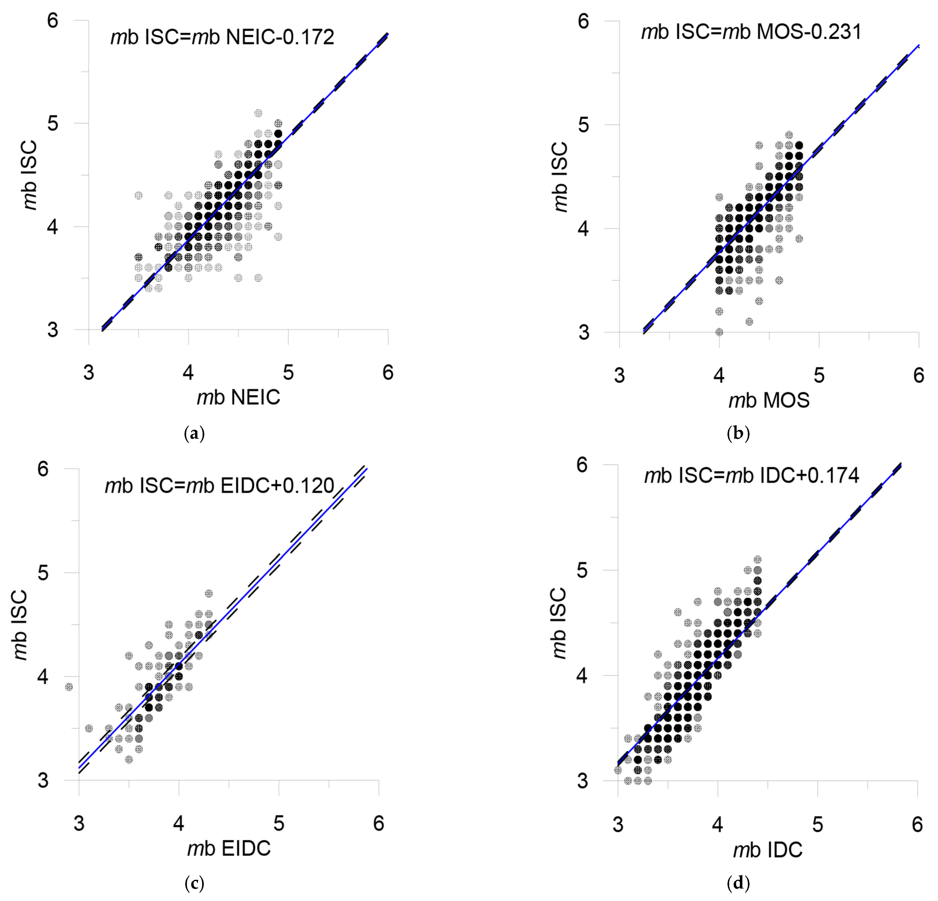
| NEIC, NEIS | mb | 4 | 27 | M = mbNEIC − 0.2 | Figure 15a | 3.5–4.9 | |
| MOS | mb | 4 | 16 | M = mbMOS − 0.2 | Figure 15b | 4.0–4.8 | |
| EIDC | mb | 4 | 24 | M = mbEIDC + 0.2 | Figure 15c | 3.0–4.3 | |
| IDC | mb | 4 | 107 | M = mbIDC + 0.2 | Figure 15d | 2.9–4.4 | |
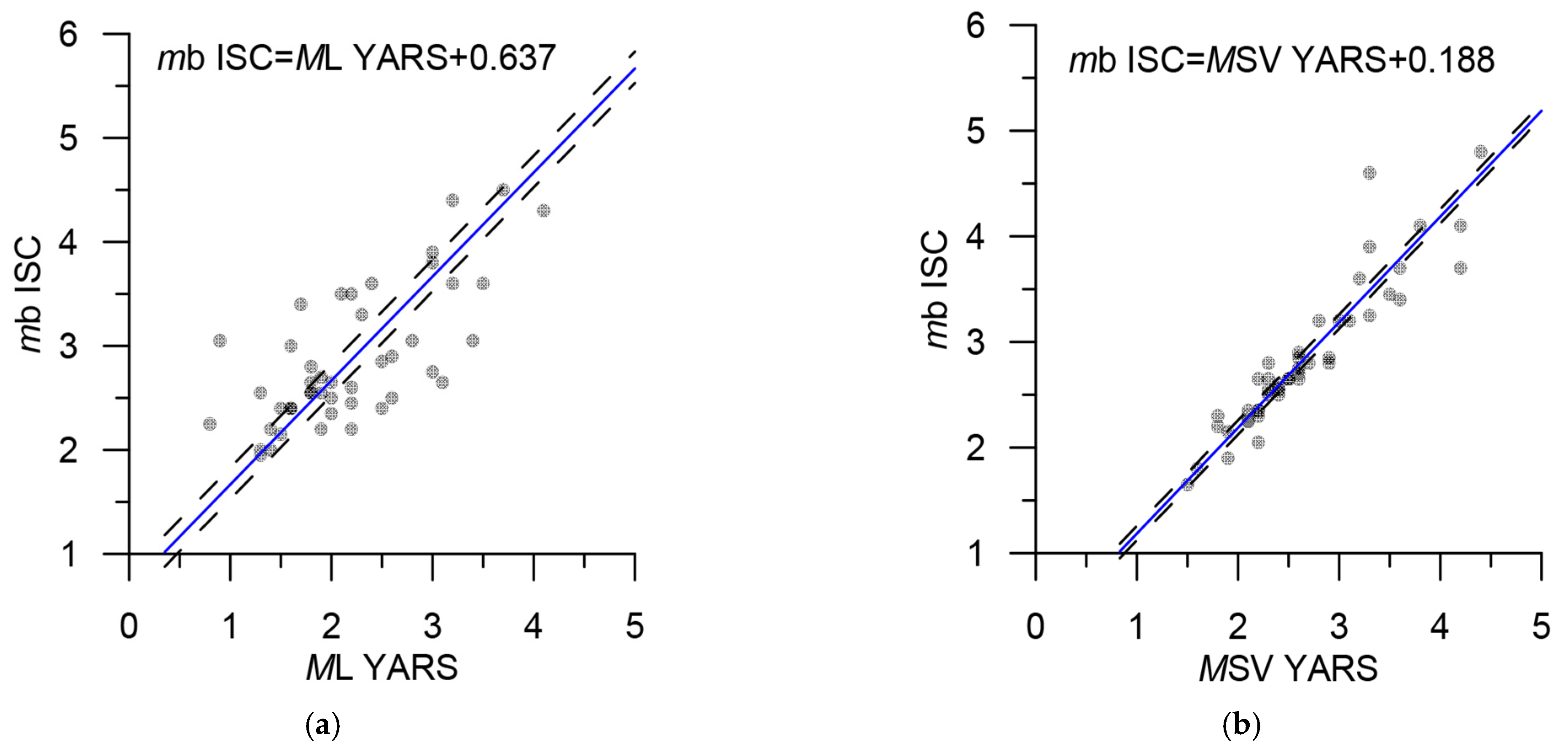
| YARS | ML | 4 | 357 | M = MLYARS + 0.6 | Figure 16a | 0.5–3.0 | Unreliable correlation |
| YARS | MSV | 4 | 95 | M = MSVYARS + 0.2 | Figure 16b | 0.0–2.1 | Unreliable correlation |
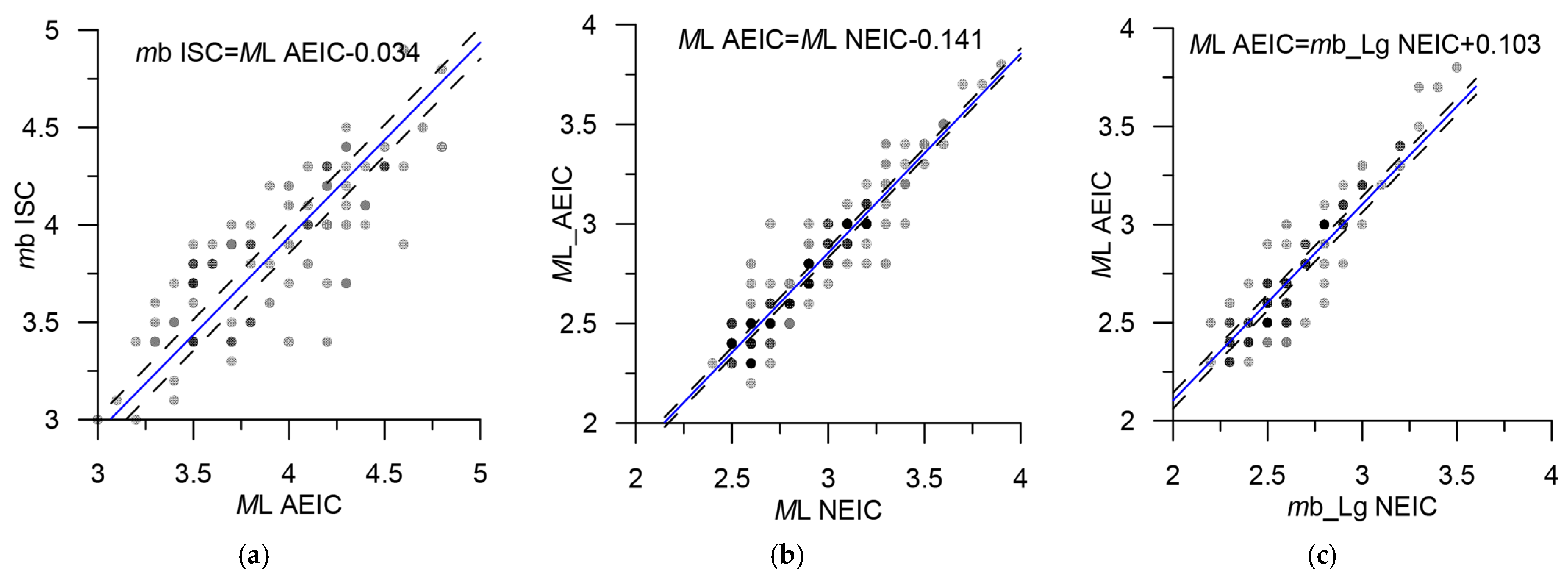
| AEIC | ML | 4 | 351 | M = MLAEIC | Figure 17a | 2.2–4.2 | |
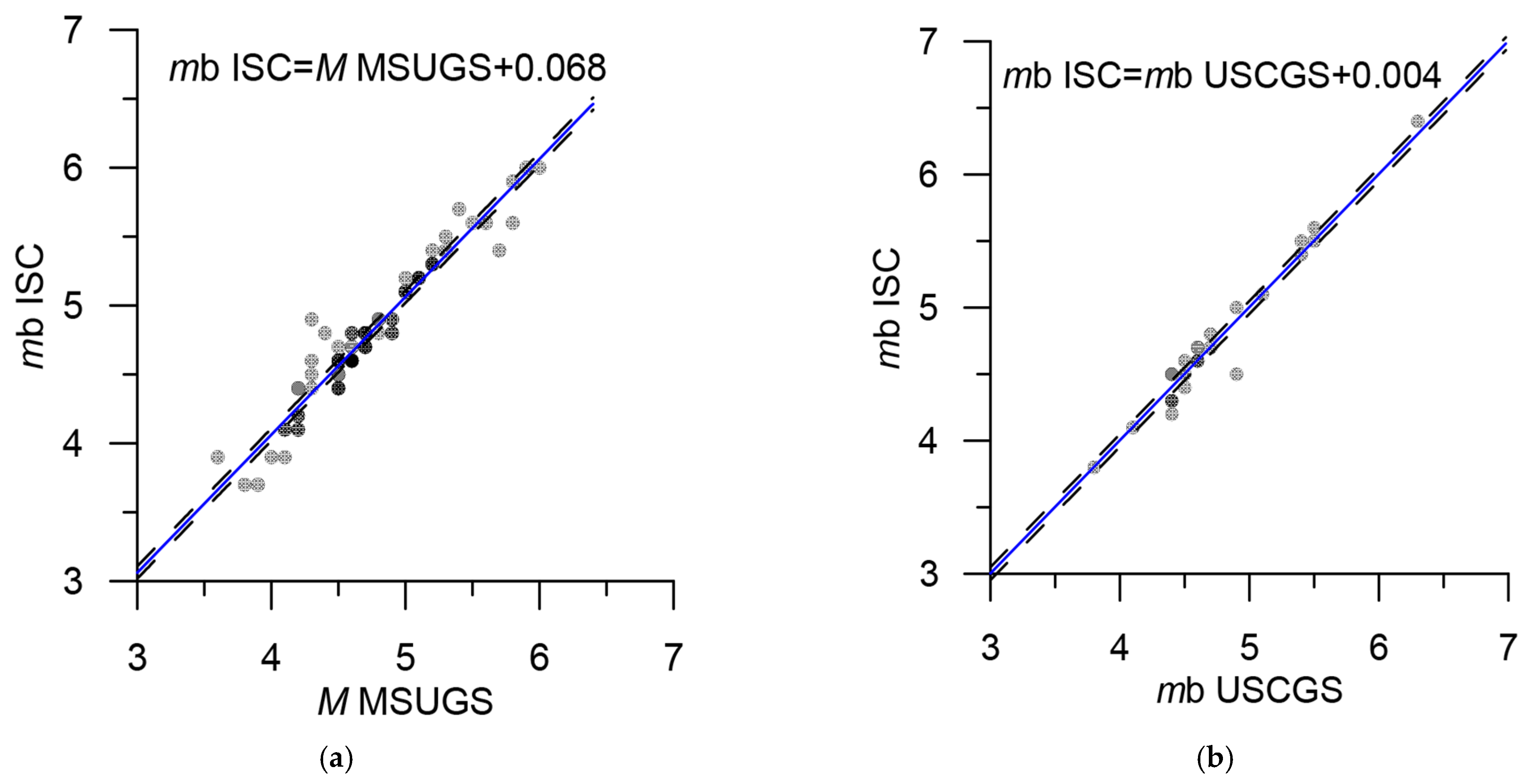
| MSUGS | M | 4 | 24 | M = MMSUGS + 0.1 | Figure 18a | 0.1–4.6 | |
| USCGS | mb | 4 | 1 | M = mbUSCGS | Figure 18b | 4.1 | Unreliable correlation |
| YARS | M | 4 | 104 | M = MYARS + 0.1 | 3.2–3.3 | Indirect correlation with energy class. The magnitude MYARS represents a conversion from the energy class KS according to the formula of Rautian MYARS = (KS − 4)/1.8. For M[3.2–3.3] up to rounding, this is a shift of 0.1. | |
| NERS | M | 4 | 24 | M = MNERS + 0.2 | 2.3–2.5 | Indirect correlation with energy class. The magnitude MNERS represents a conversion from the energy class KPS according to the formula of Rautian MNERS = (KPS − 4)/1.8. For M[2.3–2.5] up to rounding, this is a shift of 0.2. | |
| NEIC | ML | 4 | 13 | M = MLNEIC − 0.1 | Figure 17b | 2.5–4.2 | Unreliably used indirect correlation MLAEIC |
| NEIC | mbLg | 4 | 2 | M = mbLgNEIC + 0.1 | Figure 17c | 2.6–3.0 | Unreliably used indirect correlation MLAEIC |
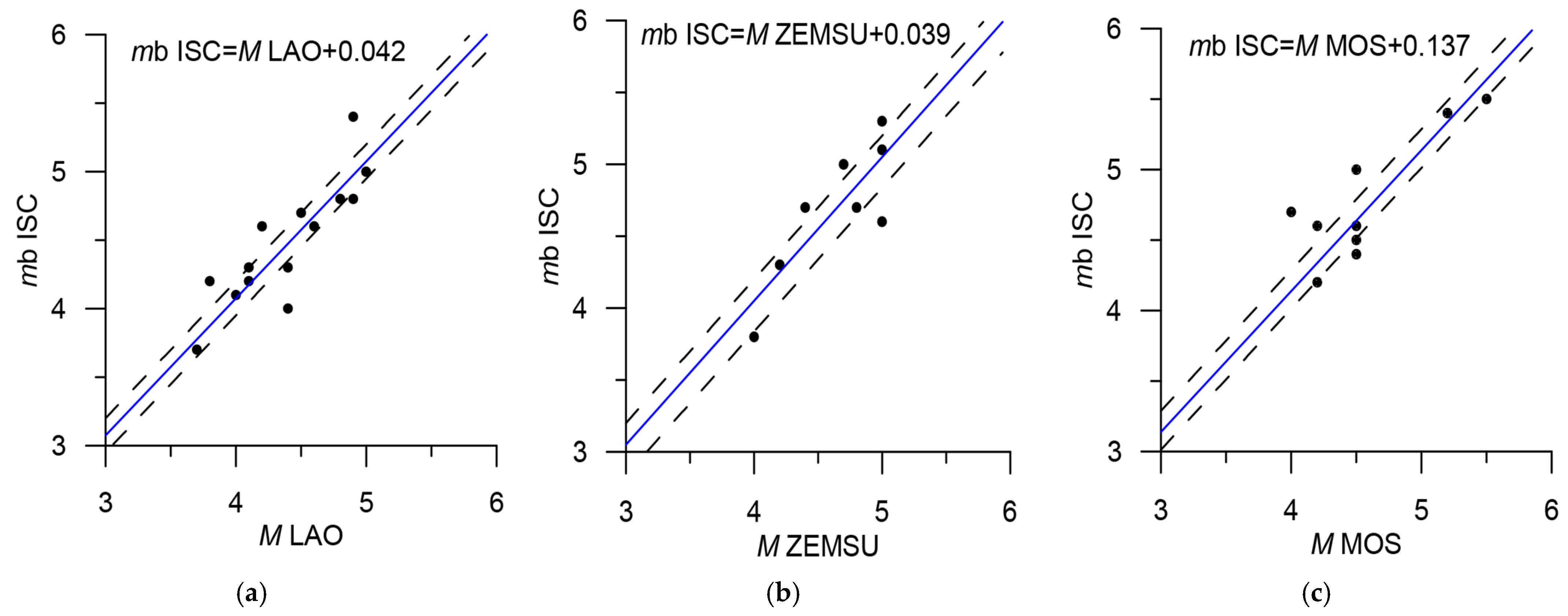
| LAO | M | 4 | 2 | M = MLAO | Figure 19a | 4.0 | Very unreliable correlation |
| ZEMSU | M | 4 | 2 | M = MZEMSU | Figure 19b | 3.4–4.5 | Very unreliable correlation |
| MOS | M | 4 | 1 | M = MMOS + 0.1 | Figure 19c | 5.0 | Very unreliable correlation |
| NEIC | M | 4 | 6 | M = MNEIC | 2.5–4.9 | Very unreliable correlation. Only three events with two magnitudes were found, MNEIC = mbISC. | |
| ANF | ML | 4 | 2 | M = MLANF − 1 | 4.2–4.3 | Very unreliable correlation. Found only two events with two magnitudes, MLANF>>mbISC. | |
| DNAG | M | 4 | 14 | M = MDNAG | 2.5–4.4 | Correlation not established | |
| WASN | M | 4 | 328 | M = MWASN | 0.1–4.4 | Correlation not established | |
| ZEMSU | MPV | 4 | 1 | M = MPVZEMSU | 4.5 | Correlation not established | |
| YARS | MU | 4 | 2 | M = MU_YARS | 1.7–2.1 | Correlation not established | |
| OTT | ML | 4 | 1 | M = MLOTT | 3.9 | Correlation not established | |
| PAL | M | 4 | 1 | M = MPAL | 4.7 | Correlation not established | |
| BJI | mb | 4 | 1 | M = mbBJI | 4.8 | Correlation not established | |
| EIDC | ML | 4 | 1 | M = MLEIDC | 2.8 | Correlation not established | |
| Total | 23,254 |
| Date | TIME | Lat | Lon | Dep | Mag | ||
|---|---|---|---|---|---|---|---|
| 1 | 22.11.1969 | 23:09:38 | 57.67 | 163.51 | 25.6 | 7.5 | MSISC |
| 2 | 18.05.1971 | 22:44:41 | 63.93 | 145.96 | 1.5 | 7.0 | MSISC |
| 3 | 08.03.1991 | 11:36:31 | 60.83 | 167.08 | 16.5 | 6.6 | MWGCMT |
| 4 | 24.10.1996 | 19:31:55 | 66.92 | −173.04 | 22.2 | 6.0 | MWGCMT |
| 5 | 20.04.2006 | 23:25:02 | 60.88 | 167.05 | 23.9 | 7.6 | MWGCMT |
| 6 | 21.04.2006 | 4:32:44 | 60.45 | 165.96 | 14.6 | 6.1 | MWGCMT |
| 7 | 21.04.2006 | 11:14:16 | 61.30 | 167.75 | 22.8 | 6.0 | MWGCMT |
| 8 | 29.04.2006 | 16:58:06 | 60.45 | 167.62 | 10.9 | 6.6 | MWGCMT |
| 9 | 22.05.2006 | 11:11:59 | 60.73 | 165.81 | 13.9 | 6.6 | MWGCMT |
| 10 | 22.06.2008 | 23:56:30 | 67.70 | 141.39 | 18.8 | 6.1 | MWGCMT |
| 11 | 30.04.2010 | 23:11:43 | 60.46 | −177.91 | 14.7 | 6.5 | MWGCMT |
| 12 | 30.04.2010 | 23:16:29 | 60.48 | −177.60 | 18.3 | 6.3 | MWGCMT |
| 13 | 24.06.2012 | 3:15:01 | 57.50 | 163.41 | 16 | 6.0 | MWGCMT |
| 14 | 14.02.2013 | 13:13:52 | 67.52 | 142.70 | 8.9 | 6.7 | MWGCMT |
| 15 | 09.01.2020 | 8:38:08 | 62.36 | 171.06 | 10 | 6.4 | MWGCMT |
Publisher’s Note: MDPI stays neutral with regard to jurisdictional claims in published maps and institutional affiliations. |
© 2022 by the authors. Licensee MDPI, Basel, Switzerland. This article is an open access article distributed under the terms and conditions of the Creative Commons Attribution (CC BY) license (https://creativecommons.org/licenses/by/4.0/).
Share and Cite
Gvishiani, A.D.; Vorobieva, I.A.; Shebalin, P.N.; Dzeboev, B.A.; Dzeranov, B.V.; Skorkina, A.A. Integrated Earthquake Catalog of the Eastern Sector of the Russian Arctic. Appl. Sci. 2022, 12, 5010. https://0-doi-org.brum.beds.ac.uk/10.3390/app12105010
Gvishiani AD, Vorobieva IA, Shebalin PN, Dzeboev BA, Dzeranov BV, Skorkina AA. Integrated Earthquake Catalog of the Eastern Sector of the Russian Arctic. Applied Sciences. 2022; 12(10):5010. https://0-doi-org.brum.beds.ac.uk/10.3390/app12105010
Chicago/Turabian StyleGvishiani, Alexei D., Inessa A. Vorobieva, Peter N. Shebalin, Boris A. Dzeboev, Boris V. Dzeranov, and Anna A. Skorkina. 2022. "Integrated Earthquake Catalog of the Eastern Sector of the Russian Arctic" Applied Sciences 12, no. 10: 5010. https://0-doi-org.brum.beds.ac.uk/10.3390/app12105010